Extraction, purification, and clumped isotope analysis of methane (Δ¹³CDH₃ and Δ¹²CD₂H₂) from sources and the atmosphere

Measurements of the clumped isotope anomalies (Δ¹³CDH₃ and Δ¹²CD₂H₂) of methane have shown potential for constraining methane sources and sinks. At Utrecht University, we use the Thermo Scientific Ultra high-resolution isotope-ratio mass spectrometer to measure the clumped isotopic composition of methane emitted from various sources and directly from the atmosphere.

We have developed an extraction system with three sections for extracting and purifying methane from high (> 1 %), medium (0.1 % to 1 %), and low-concentration (< 0.1 %) samples, including atmospheric air (∼ 2 ppm = 0.0002 %). Depending on the methane concentration, a quantity of sample gas is processed that delivers 3 ± 1 mL of pure methane, which is the quantity typically needed for one clumped isotope measurement. For atmospheric air with a methane mole fraction of 2 ppm, we currently process up to 1100 L of air.

The analysis is performed on pure methane, using a dual-inlet setup. The complete measurement time for all isotope signatures is about 20 h for one sample. The mean internal precision values of sample measurements are 0.3 ± 0.1 ‰ for Δ¹³CDH₃ and 2.4 ± 0.8 ‰ for Δ¹²CD₂H₂. The long-term reproducibility, obtained from repeated measurements of a constant target gas, over almost 3 years, is around 0.15 ‰ for Δ¹³CDH₃ and 1.2 ‰ for Δ¹²CD₂H₂. The measured clumping anomalies are calibrated via the Δ¹³CDH₃ and Δ¹²CD₂H₂ values of the reference CH₄ used for the dual-inlet measurements. These were determined through isotope equilibration experiments at temperatures between 50 and 450 °C.

We describe in detail the optimized sampling, extraction, purification, and measurement technique followed in our laboratory to measure the clumping anomalies of methane precisely and accurately. This paper highlights the extraction and one of the first global measurements of the clumping anomalies of atmospheric methane.

1 Introduction

Atmospheric methane, CH₄, is the second most important anthropogenic greenhouse gas after CO₂. The global warming potential of CH₄ is 28 times greater than that of CO₂ over a 100-year period. Having a shorter lifetime of ∼ 11 years (Li et al., 2022) compared to CO₂ (Archer et al., 2009), CH₄ responds faster to changes in its source and sink fluxes than CO₂. This also means that CH₄ emission reduction measures can have a relatively faster effect on atmospheric composition, reducing global warming. Global-scale measurements of CH₄ mole fractions show an increasing trend since pre-industrial times. The current global mean atmospheric CH₄ mole fraction as of January 2023 is 1972 ppb, while the estimated pre-industrial values were 700 to 800 ppb (Lan et al., 2022). This long-term increase is mostly attributed to anthropogenic emissions (IPCC, 2022). Precise direct atmospheric measurements have revealed significant shorter-term variations in the growth rate of atmospheric CH₄, including stable levels in the early 2000s followed by an accelerating increase since 2007. Various studies have attempted to attribute this temporal change to variations in the balance between different CH₄ sources and atmospheric sinks. However, these existing studies do not converge on the same conclusion. This shows that we do not fully understand the CH₄ cycle yet, which means that we cannot predict its future behaviour confidently.

Major CH₄ sources are often separated into these categories according to the production mechanism: biogenic (wetlands, cattle, lakes, landfills), thermogenic (natural gas, coalbed CH₄, shale gas, etc.), pyrogenic (biomass burning, combustion of fossil fuels, etc.), and abiotic (volcanic and geothermal areas, gas–water–rock interactions, etc.) sources. The main CH₄ sink in the troposphere is photochemical oxidation by OH and Cl radicals (Khalil et al., 1993). Part of the CH₄ that reaches the stratosphere is removed by Cl and O(¹D). About 10 % of the atmospheric CH₄ is taken up by surface sinks (Topp and Pattey, 1997).

A method commonly used to identify different sources and sinks of CH₄ is based on measurements of its bulk isotopic composition, denoted as δ¹³C and δD. Each source has a characteristic isotopic composition range as shown in Fig. 1a, as a result of the isotopic composition of the various substrates and the process-dependent isotopic fractionation during CH₄ formation (Whiticar et al., 1986; Whiticar, 1999; Sherwood Lollar et al., 2006; Etiope and Sherwood Lollar, 2013; Conrad, 2002; Kelly et al., 2022; Menoud et al., 2020). CH₄ from all these sources contribute to atmospheric CH₄ with an expected isotopic composition of the source mixture around −54 ‰ for δ¹³C and −290 ‰ for δD (Whiticar and Schaefer, 2007) (as shown in Fig. 1a). The sink reactions preferentially remove the lighter isotopologues of CH₄ from the atmosphere (Saueressig et al., 2001; Cantrell et al., 1990; Whitehill et al., 2017), resulting in an enrichment of the heavier isotopes in the residual CH₄. The combined effect of emissions from the various sources and removal by the different sinks lead to an overall atmospheric CH₄ bulk isotopic composition of around −48 ‰ for δ¹³C and −90 ‰ for δD. Many measurements have been performed to date, using analysis in the laboratory on collected samples and field-deployable instruments at various sites to study the variations in atmospheric CH₄ (Menoud et al., 2020, 2021, 2022; Lu et al., 2021; Beck et al., 2012; Fernandez et al., 2022; Röckmann et al., 2016a; Sherwood et al., 2017). However, due to the overlap of some of the source signatures, it is not always possible to distinguish different sources of CH₄ using the bulk isotopes (Fig. 1a).

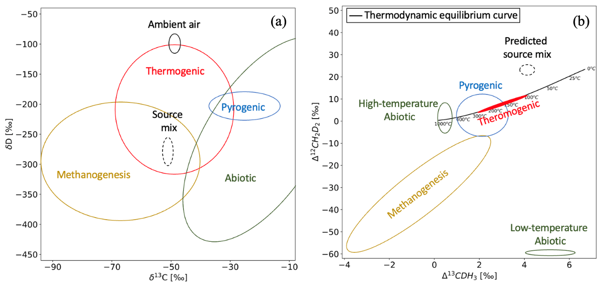
Figure 1 An illustration of bulk (a) and clumped (b) isotopic composition of major CH₄ sources as reported so far.

The measurement of the two most abundant clumped isotopologues (¹³CDH₃ and ¹²CD₂H₂) of CH₄ can be used as an additional tool to constrain CH₄ sources (Douglas et al., 2017; Eiler, 2007; Young et al., 2017; Stolper et al., 2014). The clumping anomalies, denoted as Δ¹³CDH₃ and Δ¹²CD₂H₂, are a measure of the deviation of the number of clumped molecules present relative to that expected from the random distribution of the light and heavy isotopes over all isotopologues of CH₄. At thermodynamic equilibrium, these anomalies are temperature dependent and can thus be used to calculate the CH₄ formation or equilibration temperature. In the case of thermodynamic disequilibrium, the clumped signatures can be exploited to identify various kinetic gas formation and fractionation (mixing, diffusion, etc.) processes. The clumped isotope signatures are specific to different sources and processes, independent of the bulk signatures, and thus can deliver additional information on sources and cycling of CH₄ in the environment.

Measuring the clumped isotopic composition of CH₄, however, poses several technical challenges. The ¹³CDH₃ and CD₂H₂ molecules and H₂O (which is always present in a mass spectrometer at much higher concentrations than the CH₄ clumped isotopologues) have very slightly different masses, approximately 18.0409, 18.0439, and 18.0153 amu (atomic mass unit), respectively. This difference cannot be distinguished using a conventional mass spectrometer. Also, the ¹³CH₄ and CDH₃ have the same nominal mass ($m/z$ 17), but these interferences can be circumvented by separating the C and H atoms, i.e. by converting the CH₄ to CO₂ for the δ¹³C measurements and to H₂ for δD. For clumped isotope measurements, such an approach would eliminate the signal we are looking for; thus, the measurements need to be performed on intact CH₄ molecules. In recent years, high-resolution isotope-ratio mass spectrometers have become available that can resolve these small mass differences (Eiler et al., 2013; Young et al., 2017). These new instruments can separate the ion beams around mass 18 corresponding to CH₃D⁺, ${}^{\mathrm{12}}{\mathrm{CH}}_{\mathrm{2}}{{\mathrm{D}}_{\mathrm{2}}}^{+}$, and ${{\mathrm{H}}_{\mathrm{2}}}^{\mathrm{16}}{\mathrm{O}}^{+}$, facilitating the CH₄ clumped isotope measurements.

Another challenge includes the measurement of low ion currents and the instrument stability required for long measurement times. The natural abundance of the clumped molecules is very low i.e. about $\mathrm{4.9}\times {\mathrm{10}}^{-\mathrm{6}}$ and $\mathrm{7.8}\times {\mathrm{10}}^{-\mathrm{8}}$ of the total CH₄ for ¹³CH₃D and ¹²CH₂D₂, respectively. The corresponding ion currents are proportionally low, typically around 5000 cps (counts per second) for ¹³CH₃D⁺ and 100 cps for ${}^{\mathrm{12}}{\mathrm{CH}}_{\mathrm{2}}{{\mathrm{D}}_{\mathrm{2}}}^{+}$. The cumulated number of counts control the limits of the achievable precision for the rare isotopologues. Therefore, to achieve per mil-level precision, the isotopologue ratios need to be measured for a long time. This requires several millilitres ($\mathrm{1}\mathrm{mL}\left(\text{STP}\right)=\sim \mathrm{45}\mathrm{\mu }\mathrm{mol}$, where STP represents standard temperature and pressure) of pure CH₄ for one measurement. To obtain pure CH₄ for the measurements, the samples need to be purified. Isotope fractionation can occur during sample handling, extraction, and purification, potentially introducing biases and inaccuracies in the measured bulk and clumped isotopologue ratios. Careful consideration of sample preparation methods, including minimizing fractionation and optimizing purification procedures, is crucial to ensure reliable and reproducible results. Another hurdle is that there are no readily available reference gases with known clumped isotopic composition to calibrate the measurements, so these need to be prepared.

A number of studies have reported the Δ¹³CDH₃ and Δ¹²CD₂H₂ of CH₄ from various sources, e.g. natural gas seeps, rice paddies and wetlands, lake sediments, shale gas, coal mines, natural gas leakage, and laboratory incubation experiments (Wang et al., 2015; Young et al., 2017; Stolper et al., 2018; Loyd et al., 2016; Ono et al., 2021; Giunta et al., 2019). A general overview of the expected clumped isotope signatures of CH₄ from different sources is illustrated in Fig. 1b. Thermogenic CH₄ is usually formed in thermodynamic equilibrium and therefore lies on the thermodynamic equilibrium curve between 100 and 300 °C. Biogenic CH₄ production, denoted as methanogenesis in Fig. 1b, is often characterized by disequilibrium Δ¹²CD₂H₂ values due to the kinetic isotopic fractionation associated with methanogenesis and/or combinatorial effects (Röckmann et al., 2016b; Yeung, 2016). The reported ranges of values for abiotic (produced at high and low temperatures) and pyrogenic CH₄ are also shown in Fig. 1b. The predicted clumping anomaly of the atmospheric CH₄ source mix resulting from the combination of all sources is about 4 ‰ for Δ¹³CDH₃ and 20 ‰ for Δ¹²CD₂H₂, as reported by Haghnegahdar et al. (2017) (Fig. 1b).

Recent modelling studies have suggested the potential of clumped isotope measurements of atmospheric CH₄, especially Δ¹²CD₂H₂, to distinguish between the main drivers of change in the CH₄ burden (Chung and Arnold, 2021; Haghnegahdar et al., 2017). However, as mentioned above, the clumped isotope measurements require a few millilitres (at STP) of pure CH₄. Therefore, a challenge specific to atmospheric CH₄ measurements is the extraction of CH₄ from very large samples of air required (thousands of litres).

This paper presents one of the first measurements of the clumping anomalies of atmospheric methane and provides a detailed comparison to the previously reported model predictions. The paper also describes in detail the technical setups and procedures for CH₄ clumped measurements at Utrecht University including (i) the extraction and purification of CH₄ from high- and low-concentration samples, including the extraction from large quantities of air (∼ 1000 L); (ii) calibration of measured anomalies using gas-equilibration experiments at different temperatures; (iii) the detailed settings and procedures of the actual isotope measurements using the Thermo Scientific Ultra mass spectrometer; and (iv) the data processing and calculations involved. We also report the performance of these systems so far, in terms of precision, reproducibility, stability, etc. Thus, this paper serves as a description of our measurement technique for future reference.

2 Methods

2.1 Notations, definitions, and calculations

The bulk isotopic composition of CH₄, denoted as δ¹³C and δD, is defined as follows:

$$\begin{array}{}\text{(1a)}& {\displaystyle }\mathit{\delta }{{}^{\mathrm{13}}\mathrm{C}}_{\text{sample}}={\displaystyle \frac{R_{\text{sample}}^{{}^{\mathrm{13}}\mathrm{C}}}{R_{\text{VPDB}}^{{}^{\mathrm{13}}\mathrm{C}}}}-\mathrm{1},\text{(1b)}& {\displaystyle }\mathit{\delta }{\mathrm{D}}_{\text{sample}}={\displaystyle \frac{R_{\text{sample}}^{\mathrm{D}}}{R_{\text{VSMOW}}^{\mathrm{D}}}}-\mathrm{1},\end{array}$$

where $R_{\text{sample}}^{{}^{\mathrm{13}}\mathrm{C}}$ and $R_{\text{sample}}^{\mathrm{D}}$ are the isotopic ratios of ${}^{\mathrm{13}}\mathrm{C}/{}^{\mathrm{12}}\mathrm{C}$ and $\mathrm{D}/\mathrm{H}$ of the sample, and $R_{\text{VPDB}}^{{}^{\mathrm{13}}\mathrm{C}}$ and $R_{\text{VSMOW}}^{\mathrm{D}}$ are isotopic ratios of the international standards for δ¹³C and δD (VPDB and VSMOW)¹ with their values being 0.011180 and 0.00015576, respectively (Assonov et al., 2020; Gonfiantini, 1978).

The clumped isotopic composition of CH₄ is expressed as clumping anomalies Δ¹³CDH₃ and Δ¹²CD₂H₂ relative to the clumped isotope ratio that would be obtained if the heavy isotopes, ¹³C and D, were distributed randomly across all isotopologues in the same sample:

$$\begin{array}{}\text{(2a)}& {\displaystyle }\mathrm{\Delta }{{}^{\mathrm{13}}{\mathrm{CDH}}_{\mathrm{3}}}_{\text{sample}}={\displaystyle \frac{R_{\text{sample}}^{{}^{\mathrm{13}}\mathrm{CD}}}{(\mathrm{4}\cdot R_{\text{sample}}^{{}^{\mathrm{13}}\mathrm{C}}\cdot R_{\text{sample}}^{\mathrm{D}})}}-\mathrm{1},\text{(2b)}& {\displaystyle }\mathrm{\Delta }{{}^{\mathrm{12}}{\mathrm{CD}}_{\mathrm{2}}{\mathrm{H}}_{\mathrm{2}}}_{\text{sample}}={\displaystyle \frac{R_{\text{sample}}^{\mathrm{DD}}}{(\mathrm{6}\cdot (R_{\text{sample}}^{\mathrm{D}}{)}^{\mathrm{2}})}}-\mathrm{1},\end{array}$$

where $R_{\text{sample}}^{{}^{\mathrm{13}}\mathrm{CD}}$ and $R_{\text{sample}}^{\text{DD}}$ are the isotopologue ratios of ${}^{\mathrm{13}}{\mathrm{CDH}}_{\mathrm{3}}{/}^{\mathrm{12}}{\mathrm{CH}}_{\mathrm{4}}$ and ${}^{\mathrm{12}}{\mathrm{CD}}_{\mathrm{2}}{\mathrm{H}}_{\mathrm{2}}{/}^{\mathrm{12}}{\mathrm{CH}}_{\mathrm{4}}$ of the sample, and $R_{\text{sample}}^{{}^{\mathrm{13}}\mathrm{C}}$ and $R_{\text{sample}}^{\mathrm{D}}$ are isotope ratios of ${}^{\mathrm{13}}\mathrm{C}/{}^{\mathrm{12}}\mathrm{C}$ and $\mathrm{D}/\mathrm{H}$ of the sample itself. The denominators in Eqs. (2a) and (2b) give the expected random distribution of the heavier isotopes in a sample, where 4 and 6 are symmetry factors (Young et al., 2017).

2.2 Mass spectrometer specifications and measurement methods

CH₄ bulk and clumped isotopic compositions were determined using the Thermo Scientific Ultra HR-IRMS (high-resolution isotope-ratio mass spectrometer, denoted Ultra hereafter). The prototype of the instrument was introduced by Eiler et al. (2013), and the characteristics of the Ultra at Utrecht University have been explained in detail by Adnew et al. (2019). The instrument is operated with the advanced Qtegra™ software package for data acquisition, instrument control, and data analysis.

The sample is introduced via one of the four variable-volume bellows into the ion source, and reference gas is provided from another bellows. After ionization in the ion source, the ion beam is accelerated, focused, and passed through a slit into the mass analyser. Three different slit widths of 250, 16, and 5 µm can be chosen in the standard setup, giving three resolution options: low resolution (LR), medium resolution (MR), and high resolution (HR), respectively. An additional “aperture” option can be turned on to achieve even higher resolution (HR+), wherein the focused ion beam is trimmed further in the y axis by an additional slit situated just before the electromagnet. However, increasing the resolution results in a decrease in intensity.

The ions are separated by energy and mass in the mass analyser, which leads to very well focussed ion beams, and they are collected with a variable detector array that supports one fixed and eight moveable detector platforms, which are equipped with nine Faraday detectors (L1, L2, L3, L4, centre, H1, H2, H3, H4) that can be read out with selectable resistors with resistances between 3×10⁸ Ω and 10¹³ Ω. The three collector platforms at the high mass end (H2, H3, and H4) are additionally equipped with compact discrete dynode (CDD) ion counting detectors next to the Faraday detectors.

Characterization of the Ultra for CH₄ measurements

Clumped isotope measurements of CH₄ using the Ultra are performed at high resolution (5 µm entrance slit width) with aperture, i.e. HR+ setting, to get the highest possible resolution. Two Faraday collectors are read out with resistors, 1×10¹¹ Ω for $m/z$ 16 and 1×10¹² Ω for $m/z$ 17 (¹³CH₄). To measure $m/z$ 17 (¹²CDH₃) and the clumped isotopologues at $m/z$ 18, we use the CDD of detector H4, which has a narrow detector slit. With careful tuning, the instrument can achieve mass resolving power (5 % to 95 %) higher than 42 000, which is sufficient to separate CH₄ isotopologues from each other, from contaminating isobars like H₂O⁺, OH⁺, and ${{\mathrm{NH}}_{\mathrm{3}}}^{+}$, and the adducts formed in the source, i.e. ${}^{\mathrm{12}}{{\mathrm{CH}}_{\mathrm{5}}}^{+}$, ${}^{\mathrm{13}}{{\mathrm{CH}}_{\mathrm{5}}}^{+}$, and ${}^{\mathrm{12}}{{\mathrm{CDH}}_{\mathrm{4}}}^{+}$.

As the high resolution is to a large degree achieved by using a very narrow source slit, most of the ions do not pass through the slit but deposit on the slit assembly. This leads to carbon accumulation around the slit and over time obstructs the passage of ions into the mass analyser, resulting in reduced ion transmission and sensitivity. The carbon deposits can also introduce additional scattering and deflection of ions, leading to the broadening of mass peaks and decreased mass resolution. There can also be signal instabilities due to fluctuations in ion transmission. These effects together can compromise the instrument's capability to resolve closely spaced ions. Therefore, we change the source slit regularly to avoid the impact of carbon deposits. To keep track of this, the number of counts of ${}^{\mathrm{12}}{{\mathrm{CH}}_{\mathrm{4}}}^{+}$ of each measurement is monitored (Fig. S1 in the Supplement). When the counts decrease to less than 0.5 times the counts of the first measurement using a new slit, the slit is replaced. The usual lifetime of one slit is around 6 months, depending on the number of CH₄ measurements done.

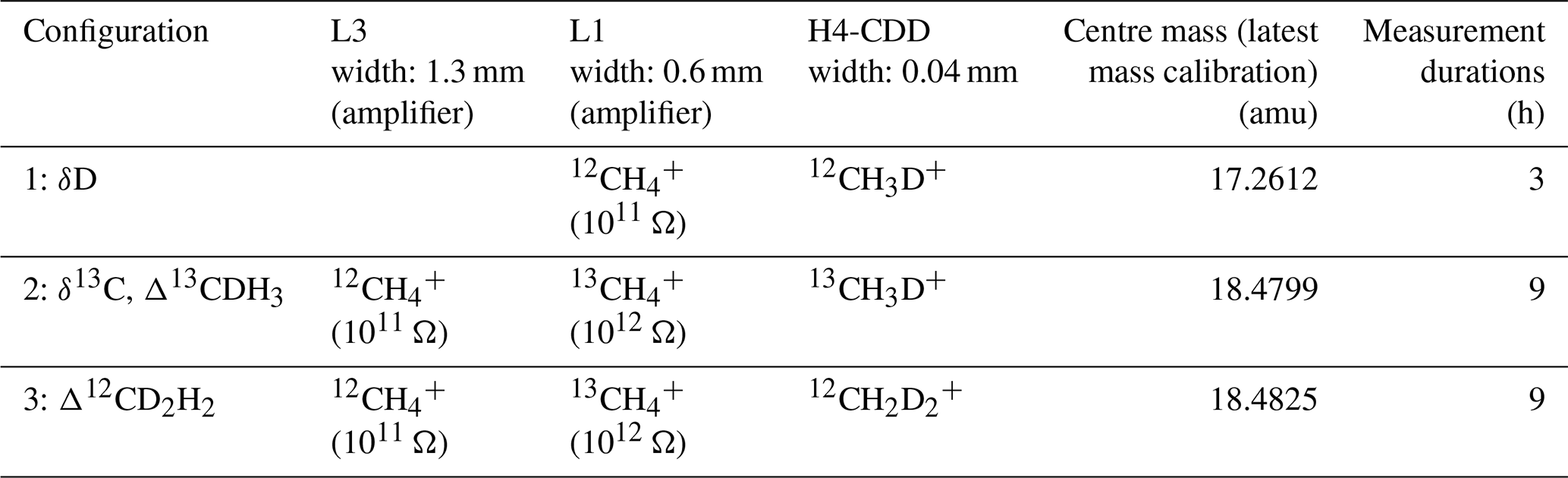
The main CH₄ isotopologues, ${}^{\mathrm{12}}{{\mathrm{CH}}_{\mathrm{4}}}^{+}$, ${}^{\mathrm{13}}{{\mathrm{CH}}_{\mathrm{4}}}^{+}$, ¹²CH₃D⁺, ¹³CH₃D⁺, and ${}^{\mathrm{12}}{\mathrm{CH}}_{\mathrm{2}}{{\mathrm{D}}_{\mathrm{2}}}^{+}$, are measured in three different configurations on the Ultra. The configurations differ by the peak centre mass setting and the relative distance between the detectors, and the peak positions are finely adjusted (Fig. 3) such that the right ions are detected by each detector. The details of the three different configurations, resistors, and detectors used for the measurements on the Ultra are given in Table 1. In the first configuration, ${}^{\mathrm{12}}{{\mathrm{CH}}_{\mathrm{4}}}^{+}$ (L1) and ¹²CH₃D⁺ (H4-CDD) are measured for about 3 h. The second configuration is set up to measure ${}^{\mathrm{12}}{{\mathrm{CH}}_{\mathrm{4}}}^{+}$ (L3), ${}^{\mathrm{13}}{{\mathrm{CH}}_{\mathrm{4}}}^{+}$ (L1), and ¹³CH₃D⁺ (H4-CDD), and the third configuration measures ${}^{\mathrm{12}}{{\mathrm{CH}}_{\mathrm{4}}}^{+}$ (L3), ${}^{\mathrm{13}}{{\mathrm{CH}}_{\mathrm{4}}}^{+}$ (L1), and ${}^{\mathrm{12}}{\mathrm{CH}}_{\mathrm{2}}{{\mathrm{D}}_{\mathrm{2}}}^{+}$ (H4-CDD). Configurations 2 and 3 are measured alternately for 18 h in seven cycles each lasting about 2.5 h. Therefore, in total, one complete measurement of all three configurations takes about 20 h. The sample and reference gases are measured alternately, each three times (meaning integrations) for a total of 201.3 s; the average of which is considered one data point. The result of one complete measurement is the average of all the data measured (outliers removed), and the internal precision is the standard error over these data points.

Table 1 The details of the three different configurations, resistors, and detectors used for the measurements on the Ultra.

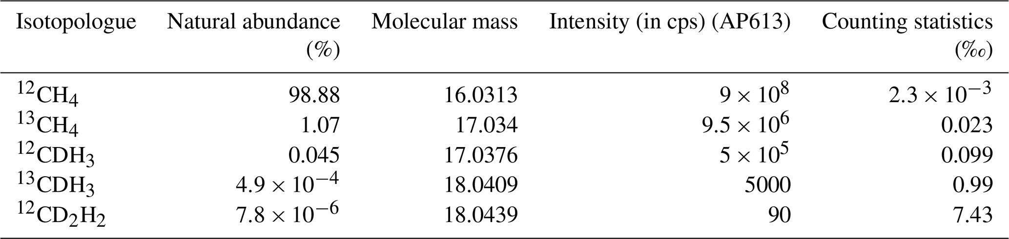
A summary of the natural abundances, molecular masses, expected intensity (in cps) (for AP613, the laboratory reference gas), and the counting statistics precision limit for all five isotopologues is given in Table 2.

Table 2 A summary of the natural abundances, molecular masses, expected intensity (in cps) (for AP613, the laboratory reference gas), and the counting statistics precision limit for an integration time of 201.3 s for all five isotopologues of CH₄ measured on the Ultra.

The gases are measured at a source pressure of maximum $\mathrm{2.5}\times {\mathrm{10}}^{-\mathrm{7}}$ mbar. The pressure in the source is controlled by the bellows pressure, which can be set and adjusted using Qtegra. The typical pressure in the bellows required to achieve this source pressure for CH₄ is around 65 to 70 mbar. We use a continuous pressure adjustment method, which means, after each integration, the bellows pressures are checked five times, and the bellows are compressed by 0.5 % each time, until the set value is attained. The tolerance of the pressure adjustment is set to 0.5 mbar, so the signal is stable within ± 0.7 %. This ensures that the instrument measures the reference and sample at the same source pressure during the entire (more than) 20 h of measurement time.

All measurements are made relative to a reference gas, which is a stainless-steel (SS) canister filled from a high purity (> 99.999 %) CH₄ reference gas cylinder (AP613). The sample and the reference are measured alternately, and then the bulk and clumped isotopic composition of the samples are calculated from the isotopologue ratios as follows:

$$\begin{array}{}\text{(3a)}& {\displaystyle }{\mathit{\delta }}_{\text{sam-VPDB}}^{{}^{\mathrm{13}}\mathrm{C}}={\mathit{\delta }}_{\text{sam-ref}}^{{}^{\mathrm{13}}\mathrm{C}}+{\mathit{\delta }}_{\text{ref-VPDB}}^{{}^{\mathrm{13}}\mathrm{C}}+\left({\mathit{\delta }}_{\text{sam-ref}}^{{}^{\mathrm{13}}\mathrm{C}}\cdot {\mathit{\delta }}_{\text{ref-VPDB}}^{{}^{\mathrm{13}}\mathrm{C}}\right),\text{(3b)}& {\displaystyle }\begin{array}{rl}{\mathit{\delta }}_{\text{sam-VSMOW}}^{\mathrm{D}}& ={\mathit{\delta }}_{\text{sam-ref}}^{\mathrm{D}}+{\mathit{\delta }}_{\text{ref-VPDB}}^{\mathrm{D}}\\ & +\left({\mathit{\delta }}_{\text{sam-ref}}^{\mathrm{D}}\cdot {\mathit{\delta }}_{\text{ref-VSMOW}}^{\mathrm{D}}\right),\end{array}\text{(3c)}& {\displaystyle }{\mathrm{\Delta }}_{\text{sam}}^{{}^{\mathrm{13}}{\mathrm{CDH}}_{\mathrm{3}}}={\displaystyle \frac{\left(\mathrm{1}+{\mathit{\delta }}_{\text{sam-ref}}^{{}^{\mathrm{13}}{\mathrm{CDH}}_{\mathrm{3}}}\right)\cdot \left(\mathrm{1}+{\mathrm{\Delta }}_{\text{ref}}^{{}^{\mathrm{13}}{\mathrm{CDH}}_{\mathrm{3}}}\right)}{\left(\mathrm{1}+{\mathit{\delta }}_{\text{sam-ref}}^{{}^{\mathrm{13}}\mathrm{C}}\right)\cdot \left(\mathrm{1}+{\mathit{\delta }}_{\text{sam-ref}}^{\mathrm{D}}\right)}}-\mathrm{1},\text{(3d)}& {\displaystyle }{\mathrm{\Delta }}_{\text{sam}}^{{}^{\mathrm{12}}{\mathrm{CD}}_{\mathrm{2}}{\mathrm{H}}_{\mathrm{2}}}={\displaystyle \frac{\left(\mathrm{1}+{\mathit{\delta }}_{\text{sam-ref}}^{{}^{\mathrm{12}}{\mathrm{CD}}_{\mathrm{2}}{\mathrm{H}}_{\mathrm{2}}}\right)\cdot \left(\mathrm{1}+{\mathrm{\Delta }}_{\text{ref}}^{{}^{\mathrm{12}}{\mathrm{CD}}_{\mathrm{2}}{\mathrm{H}}_{\mathrm{2}}}\right)}{{\left(\mathrm{1}+{\mathit{\delta }}_{\text{sam-ref}}^{\mathrm{D}}\right)}^{\mathrm{2}}}}-\mathrm{1},\end{array}$$

where ${\mathit{\delta }}_{\text{sam-ref}}^{{}^{\mathrm{13}}\mathrm{C}}$, ${\mathit{\delta }}_{\text{sam-ref}}^{\mathrm{D}}$, ${\mathit{\delta }}_{\text{sam-ref}}^{{}^{\mathrm{13}}{\mathrm{CDH}}_{\mathrm{3}}}$, and ${\mathit{\delta }}_{\text{sam-ref}}^{{}^{\mathrm{12}}{\mathrm{CD}}_{\mathrm{2}}{\mathrm{H}}_{\mathrm{2}}}$ are the values of the sample measured against the reference calculated from the measured ion intensities on the Ultra. These values are converted to the standard scales: ${\mathit{\delta }}_{\text{sam-VPDB}}^{{}^{\mathrm{13}}\mathrm{C}}$, ${\mathit{\delta }}_{\text{sam-VSMOW}}^{\mathrm{D}}$, ${\mathrm{\Delta }}_{\text{sam}}^{{}^{\mathrm{13}}{\mathrm{CDH}}_{\mathrm{3}}}$, and ${\mathrm{\Delta }}_{\text{sam}}^{{}^{\mathrm{12}}{\mathrm{CD}}_{\mathrm{2}}{\mathrm{H}}_{\mathrm{2}}}$ using the formulae above. The clumping anomalies of the reference gas used for the measurements, AP613, denoted as ${\mathrm{\Delta }}_{\text{ref}}^{{}^{\mathrm{13}}{\mathrm{CDH}}_{\mathrm{3}}}$ and ${\mathrm{\Delta }}_{\text{ref}}^{{}^{\mathrm{12}}{\mathrm{CD}}_{\mathrm{2}}{\mathrm{H}}_{\mathrm{2}}}$, were assigned using temperature-equilibration experiments which are explained in detail in the next section. The bulk isotopic composition of AP613, denoted as ${\mathit{\delta }}_{\text{ref-VPDB}}^{{}^{\mathrm{13}}\mathrm{C}}$ and ${\mathit{\delta }}_{\text{ref-VSMOW}}^{\mathrm{D}}$, was obtained by measurements using a conventional continuous-flow IRMS system (Menoud et al., 2021).

2.3 Temperature calibration scale

To produce a CH₄-clumped isotope calibration scale, we performed a series of isotope exchange experiments at various temperatures. For this, the laboratory reference gas AP613 was used, which is a commercially available pure CH₄ gas cylinder with known bulk isotopic composition. CH₄ from AP613 was equilibrated at temperatures ranging from 50 to 450 °C using two different catalysts: γ-Al₂O₃ for temperatures below 200 °C and Pt on Al₂O₃ for 200 to 450 °C.

Both catalysts were activated using the procedure explained in Eldridge et al. (2019). For each heating experiment, about 10 pellets of the catalyst were inserted into a 20 mL glass tube with a Teflon valve and evacuated to 10⁻³ mbar to remove adsorbed air and moisture. The tube was then filled with 140 mbar of pure O₂ and heated for about 5 h at 550 °C for activation of the catalyst. After heating, the tube was evacuated overnight (for 12 to 14 h) at 550 °C and then cooled to room temperature. The pellets were not exposed to outside air once activated. After the activated pellets were cooled to room temperature, 5 to 6 mL of pure CH₄ (AP613) was added to the tube and heated at the desired temperature and duration as given in Table 3.

Table 3 Summary of the equilibrated gas experiments; Δ¹³CDH₃ raw and Δ¹²CD₂H₂ raw values are relative to the reference gas, and Δ¹³CDH₃ absolute and Δ¹²CD₂H₂ absolute are calculated using the assigned anomalies of the reference gas.

The equilibrated gases were measured on the Ultra against the reference gas, i.e. unmodified CH₄ from the AP613 cylinder. The raw Δ¹³CDH₃ and Δ¹²CD₂H₂ values are calculated using Eqs. (3c) and (3d) but assuming ${\mathrm{\Delta }}_{\text{ref}}^{{}^{\mathrm{13}}{\mathrm{CDH}}_{\mathrm{3}}}$ and ${\mathrm{\Delta }}_{\text{ref}}^{{}^{\mathrm{12}}{\mathrm{CD}}_{\mathrm{2}}{\mathrm{H}}_{\mathrm{2}}}$ to be zero. The raw values obtained in this way showed the expected dependence on temperature but with a shift due to the real clumped values of the reference being different from zero. To determine this offset, the functions from Eldridge et al. (2019) were fit to the data with an added free parameter for the offset as given in Eqs. (4a) and (4b):

$$\begin{array}{}\text{(4a)}& {\displaystyle }\begin{array}{rl}\mathrm{\Delta }{}^{\mathrm{13}}{\mathrm{CDH}}_{\mathrm{3}}& =a+{\displaystyle \frac{\mathrm{1.47348}\times {\mathrm{10}}^{\mathrm{19}}}{T^{\mathrm{7}}}}-{\displaystyle \frac{\mathrm{2.08648}\times {\mathrm{10}}^{\mathrm{17}}}{T^{\mathrm{6}}}}\\ & +{\displaystyle \frac{\mathrm{1.1981}\times {\mathrm{10}}^{\mathrm{17}}}{T^{\mathrm{5}}}}-{\displaystyle \frac{\mathrm{3.54757}\times {\mathrm{10}}^{\mathrm{12}}}{T^{\mathrm{4}}}}\\ & +{\displaystyle \frac{\mathrm{5.54476}\times {\mathrm{10}}^{\mathrm{9}}}{T^{\mathrm{3}}}}-{\displaystyle \frac{\mathrm{3.49294}\times {\mathrm{10}}^{\mathrm{6}}}{T^{\mathrm{2}}}}\\ & +{\displaystyle \frac{\mathrm{8.8937}\times {\mathrm{10}}^{\mathrm{2}}}{T}},\end{array}\text{(4b)}& {\displaystyle }\begin{array}{rl}\mathrm{\Delta }{}^{\mathrm{12}}{\mathrm{CD}}_{\mathrm{2}}{\mathrm{H}}_{\mathrm{2}}& =b-{\displaystyle \frac{\mathrm{9.67634}\times {\mathrm{10}}^{\mathrm{15}}}{T^{\mathrm{6}}}}+{\displaystyle \frac{\mathrm{1.71917}\times {\mathrm{10}}^{\mathrm{14}}}{T^{\mathrm{5}}}}\\ & -{\displaystyle \frac{\mathrm{1.24819}\times {\mathrm{10}}^{\mathrm{12}}}{T^{\mathrm{4}}}}+{\displaystyle \frac{\mathrm{4.30283}\times {\mathrm{10}}^{\mathrm{9}}}{T^{\mathrm{3}}}}\\ & -{\displaystyle \frac{\mathrm{4.4866}\times {\mathrm{10}}^{\mathrm{6}}}{T^{\mathrm{2}}}}+{\displaystyle \frac{\mathrm{1.86258}\times {\mathrm{10}}^{\mathrm{3}}}{T}}.\end{array}\end{array}$$

The parameters a and b were then optimized, keeping the shape of the temperature dependence constant, and they were used to estimate the Δ¹³CDH₃ and Δ¹²CD₂H₂ values of our reference gas. In practice, this was done using a Monte Carlo simulation with 1000 runs: at each run, each data point was independently applied with a random error based on the uncertainty of that measurement, assuming Gaussian distribution of the errors. The functions above were then fitted, and a set of free parameters (a and b) were obtained. The final absolute Δ¹³CDH₃ and Δ¹²CD₂H₂ values of the reference were calculated by averaging the a and b parameters for all runs (with outliers removed), and the errors reported are the corresponding standard deviations.

2.4 CH₄ extraction and purification system

The schematic of the extraction system is shown in Fig. 2.

Figure 2 Schematic of high-concentration extraction system (HCES) and low-concentration extraction system (LCES) and the GC setup at IMAU. Samples are introduced to the HCES via H4 and to the LCES via L0. The pre-concentrated sample in CT2 is transferred to Trap A via a connection between L12 and H2. The acronyms used in the figures are explained in the main text (Sect. 2.4).

Precise measurements of the clumped isotopic composition of CH₄ on the Ultra require about 3 ± 1 mL of pure CH₄ for a single measurement. Throughout this paper, the quantity of gas is specified in millilitres (mL) (at STP, unless otherwise specified; the conversion to molar units is $\mathrm{1}\mathrm{mL}=\sim \mathrm{45}\mathrm{\mu }\mathrm{mol}$).

The CH₄ extraction and preconcentration procedure followed in our laboratory involves several steps depending on the sample concentration as explained below.

2.4.1 HCES

The high-concentration extraction system (HCES) is used to extract CH₄ from samples with more than 1 % of CH₄, i.e. extracting from up to 200 mL of sample gas. The HCES includes two empty traps (Trap C and Trap D), two traps filled with silica gel (Trap A and Trap B), and a gas chromatograph (GC) with a passive thermal conductivity detector (TCD), all connected with $\mathrm{1}/\mathrm{4}$ in. SS tubing and 316 L VIM-VAR Swagelok valves. All the parts are shown in the schematic (Fig. 2). This system is built following the one described in Young et al. (2017).

The CH₄ in the sample gas is separated from the other components by GC, and then it is collected cryogenically on silica gel. The sample is introduced via valve H4 and collected in Trap A with silica gel cooled to −196 °C with liquid N₂. The pressure in the system is monitored to ensure that all the sample is trapped. The sample in Trap A is introduced to the GC from Trap A using He at a flow rate of 30 mL min⁻¹ for 5 min by warming the trap to about 70 °C using a hot water bath.

The GC has two columns used in series for the final purification of CH₄: A 5 m $\mathrm{1}/\mathrm{4}$ in. o.d. SS column packed with a 5 Å molecular sieve to separate H₂, Ar, O₂, and N₂ from hydrocarbons and a 2 m $\mathrm{1}/\mathrm{4}$ in. o.d. SS column packed with HayeSep D porous polymer to separate CH₄ from the remaining higher hydrocarbons like C₂H₆, C₃H₈, etc. Wide columns of $\mathrm{1}/\mathrm{4}$ in. are used to attain separation of more than 5 mL of CH₄ within 55 min.

CH₄ elutes from the GC column after O₂, N₂, and Kr. For concentrated samples (> 5 % CH₄ in air) without Kr, O₂ elutes around 10 min, N₂ around 22 min, and CH₄ around 40 min when the GC is operated at 50 °C. After the complete elution of N₂ (35 min), Trap B with silica gel is cooled with liquid N₂ to collect CH₄ for about 15 min. Once all the CH₄ is collected, Trap B is evacuated for 10 min to remove the He carrier gas while the trap is still cooled with liquid N₂. Following this, CH₄ is released from Trap B by warming the trap to ∼ 70 °C (hot water bath) and collected in a sample vial filled with silica gel and cooled with liquid N₂ to be transferred to the mass spectrometer.

For samples with CH₄ concentrations between 1 % and 5 % CH₄ in air, the sample volumes required to extract the required amount of CH₄ are larger (> 100 mL). In this case, the O₂ and N₂ peaks are not fully resolved and not well separated from CH₄. Therefore, CH₄ along with traces of O₂ and N₂ eluted from the GC is collected in Trap A instead of the sample vial and passed through the GC a second time for further purification (same steps as above). In the second round of extraction, the O₂ and N₂ peaks are small and well separated from each other and from the CH₄ peak. For samples with ppm levels of Kr (notably atmospheric samples), separation of pure CH₄ from Kr was only achieved when the GC columns were heated at 40 °C instead of 50 °C normally used for other samples. The comparison of chromatograms before and after Kr separation was achieved is shown in Fig. 9.

After each chromatographic separation, the GC columns are baked at 200 °C for 30 min with He flow to remove CO₂, the heavier hydrocarbons, and other impurities. After baking, the columns are slowly cooled to 50 °C for the next extraction. Traps A and B are heated overnight at 150 °C while pumping with a high-vacuum pump. The silica gel flask used for sample collection is evacuated until the next use.

2.4.2 LCES

Extracting CH₄ from large quantities of air involves a stepwise increase of the CH₄ concentration by cryogenically trapping the sample gas in successively smaller charcoal traps, until the concentration is high enough for the sample to be further processed with the HCES. The low-concentration extraction system (LCES) is made of a $\mathrm{1}/\mathrm{2}$ in. glass tube with J. Young high-vacuum PTFE valves, and the major components are an empty glass trap (GT), two Russian doll traps (RDT1 and RDT2), and two charcoal traps (CT1 and CT2) as shown in Fig. 2. A part of the LCES is from the extraction system that has been used previously for CO isotope analysis (Bergamaschi et al., 2000, 1998).

The GT and RDTs are respectively used to remove H₂O and CO₂ from the air. This is followed by two pre-concentration steps in CT1 and CT2, which both collect all the CH₄ but only a small part of bulk air so that the CH₄ concentration increases in each step. The exhaust of the low-vacuum pump which draws the air though the extraction system is connected to a G2301 greenhouse gas analyser (Picarro Inc.) to monitor CO₂, CH₄, and H₂O concentrations during the whole extraction procedure. This ensures that a potential breakthrough is detected.

The air taken directly from outside or from a cylinder is first dried using the GT cooled to −70 °C with a dry ice and ethanol slurry. A Mg(ClO₄)₂ tube after the GT further dries the air sample before it is introduced to the traps for collection. RDT1 and RDT2, both cooled to −196 °C with liquid N₂ and connected in series, are used to scrub CO₂, N₂O, H₂O, traces, and other condensable gases from the air. The CO₂-free air is then passed through CT1 (−196 °C), which traps CH₄ quantitatively, and only part of the remaining air components (O₂, N₂, etc.). During this CT1 collection period, CT2 is bypassed. The flow of air is controlled using a mass flow controller (MFC 1) and is adjusted to 6 to 6.5 L min⁻¹ to maintain a pressure lower than 230 mbar in the glass line between L1 and L6 to avoid condensation of O₂ in the traps cooled with liquid N₂, which is a potential danger. The glass line is partially heated using heating wires to avoid freezing of tubes and valves.

Once a quantity of about 1100 L of air has been processed, the remaining air in the glass line is pumped until P4 drops to 4 mbar. To transfer the collected air from CT1 to CT2, the liquid N₂ around CT1 is replaced with a dry ice + EtOH slurry to warm the trap to −70 °C. At this temperature, the emerging N₂+O₂ mixture is pumped out for 3 to 4 min, while the CH₄ stays in the CT1 trap. In the meantime, the bypassed CT2 is cooled to −196 °C with liquid N₂. The remaining gas mix in CT1 is released by removing the dry ice slurry and heating CT1 with a hot water bath and is passed through CT2 (−196 °C). As the pressure in the line drops to 10 mbar, 0.5 L min⁻¹ of additional pure N₂ is used to transfer any remaining gas from CT1 to CT2 for 5 min via MFC 1. After this, the liquid N₂ bath of CT2 is replaced with dry ice + EtOH slurry and pumped for 1 to 2 min to further concentrate the air mixture. At the end of this step, the final sample volume is less than 100 mL, and the sample can be transferred to Trap A of the HCES, cooled with liquid N₂. CT2 is heated using a water bath, and, after the pressure reading on P3 drops to 0 mbar, it is flushed with pure N₂ from MFC 3 (at 5 mL min⁻¹ for 2 min) to transfer the remaining gas. Once all the sample is collected in Trap A, the high-concentration extraction procedure is followed as explained above.

For samples with medium concentrations (0.1 % to 1 % CH₄) i.e. < 3 L total sample volume, the first few steps of the LCES are skipped, and the sample is directly trapped in CT2. The remaining procedure is the same as explained above.

Before each extraction, RDTs and CTs are cleaned using 0.5 L min⁻¹ of pure N₂ for 40 min while heating them with hot water baths at 70 °C to avoid contamination from the previous sample.

2.4.3 Extraction system tests with laboratory reference gas

The extraction and purification system was tested using three of our laboratory reference gases: AP613, CAL1549, and IMAU-3. Various mixtures of pure AP613 in zero air (synthetic air: O₂+N₂) and pure CAL1549 in zero air were used to test the extraction system, and then the extracted CH₄ was measured on the Ultra. The separation of Kr from CH₄ in the GC and the effect of Kr on the isotope measurements on the Ultra were tested using a 1:1 mixture of IMAU-3 and pure Kr.

To replicate the atmospheric CH₄ samples, pure AP613 was mixed with zero air to a mole fraction of 2.5 ppm of methane in 1000 L. Since zero air is devoid of CO₂ and H₂O, GT and RDT2 were bypassed for these tests. RDT1 was still immersed in liquid N₂ to ensure that even small traces of CO₂ were trapped and to check that the RDTs do not influence the clumping anomalies of CH₄. The rest of the procedure was followed as for normal sampling.

2.5 Quality checks for the Ultra

To establish the accuracy of the Ultra measurements, the Ultra δD and δ¹³C measurements were compared to conventional bulk isotope measurements. Most samples were analysed for δD and δ¹³C before the extraction and purification, using an independent conventional bulk isotope measurement system (Menoud et al., 2020), and the results were compared to the ones obtained from the Ultra measurements after the extraction.

Weekly “zero enrichment” measurements (same gas in both bellows) were done to check for systematic differences between the bellows (e.g. by contamination, leaks). These, together with regular measurements of the pure CAL1549 gas, were used to monitor the stability of the instrument and the reproducibility of the measurements. The internal precision of the measurements was estimated for each measurement (sample or test gas) from the 1 SE (standard error) over the whole measurement.

An inter-laboratory comparison with the Nu Panorama high-resolution mass spectrometer operated at the University of Maryland (UMD) was done for the three laboratory reference gases: AP613, CAL1549, and IMAU-3. The results of these comparisons are presented in the next section.

3 Results and discussion

3.1 Ultra measurements

As described in Sect. 2.2, clumped isotope measurements on the Ultra involve measuring the different isotopologues in three configurations for a total of 20 h. Typical mass scans of the three configurations are shown in Fig. 3. The position of the peak centres (marked with red dotted lines in Fig. 3) is quite stable during the entire measurement procedure and small mass shifts are corrected every hour using the peak centre correction feature in the software.

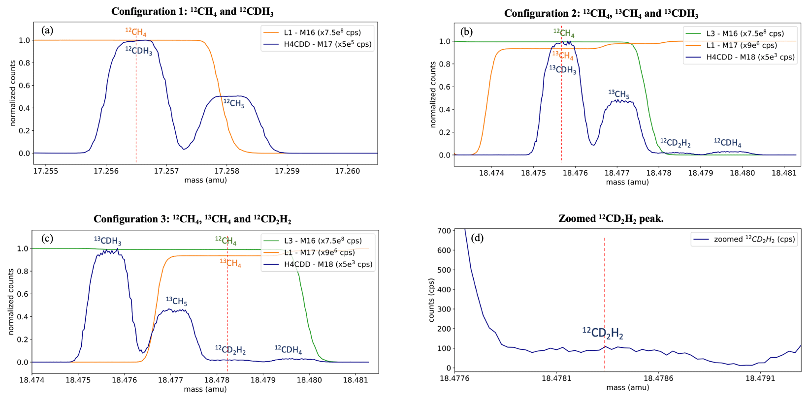
Figure 3 Mass scans of three configurations to measure ¹²CDH₃ (a), ¹³CH₄ and ¹³CDH₃ (b), and ¹³CH₄ and ¹²CD₂H₂ (c, d). The x axis values correspond to the peak centre setting, i.e. mass 17 in panel (a) and mass 18 in panels (b)–(d), and the other detectors are offset to these values to show the other isotopologues on the same scale. The different detectors used, and the normalization factors are given in the legends. The dashed red line indicates the peak centre mass setting. Panel (d) shows the zoomed-in peak of ¹²CD₂H₂ and the counts measured.

3.2 Temperature equilibration experiments

The results of the heating experiments are presented in Table 3. The equilibrated gas (subsample of AP613 heated at different temperatures; Sect. 2.3) was measured against the non-equilibrated gas from AP613 (directly from the cylinder), which is the Ultra reference gas. Raw measurement values relative to the reference gas are reported as Δ¹³CDH₃ raw and Δ¹²CD₂H₂ raw.

The measured values of heated AP613 at different temperatures were compared to the theoretical equilibrium curve, and the Δ¹³CDH₃ and Δ¹²CD₂H₂ values of AP613 were estimated using the Monte Carlo simulations as described in Sect. 2.3. The Δ¹³CDH₃ and Δ¹²CD₂H₂ assigned to our reference gas, AP613, are the following: Δ¹³CDH₃=2.23 ± 0.12 ‰ and Δ¹²CD₂H₂=3.1 ± 0.9 ‰. Since this pair of values for the clumping anomalies does not lie on the thermodynamic equilibrium curve, we cannot assign a formation temperature value to AP613. The absolute values of Δ¹³CDH₃ and Δ¹²CD₂H₂ calculated using the assigned values of AP613 are given in Table 3 and in Fig. 4.

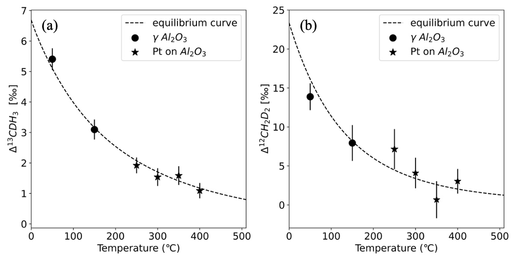
Figure 4 Absolute Δ¹³CDH₃ and Δ¹²CD₂H₂ of the equilibrated gas compared to the theoretical equilibrium curve, calculated using the assigned anomalies of the reference gas, AP613: Δ¹³CDH₃=2.23 ± 0.12 ‰ and Δ¹²CD₂H₂=3.1 ± 0.9 ‰. The data points represent the equilibrated gas at different temperatures with the markers corresponding to the different catalysts as given in the legend. The dashed black line is the thermodynamic equilibrium curve.

3.3 Internal precision and reproducibility of the Ultra measurements

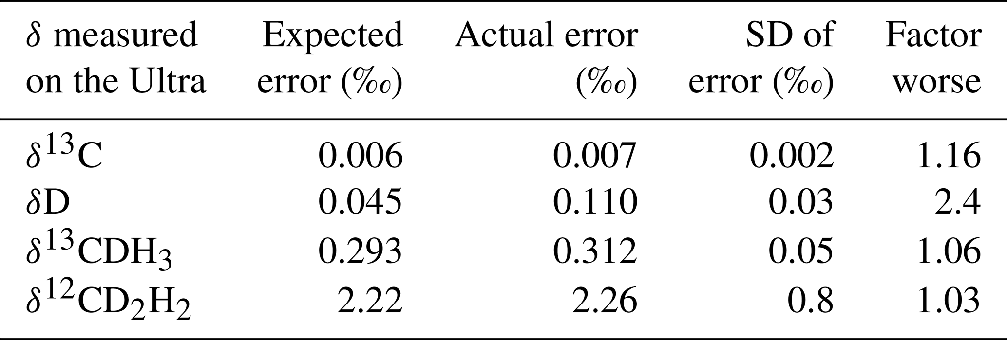
The average standard errors of the measured δ¹³C, δD, δ¹³CDH₃, and δ¹²CD₂H₂ values and their comparison to the expected precision based on counting statistics of the shot noise are given in Table 4. Achieved precisions are very close to the shot noise limit for δ¹³C, δ¹³CDH₃, and δ¹²CD₂H₂. Typically, δD measurements are about 2 times worse than the shot noise limit. This may be because of the following reasons: the high count rates (of the order of 10⁵) of ¹²CH₃D measured using the H4-CDD detector are close to the upper limit of the CDD operating range, and they are not in the optimal region. Therefore, we expect here a lower signal-to-noise ratio (meaning a higher relative error). Additionally, the peak top of ¹²CH₃D, which is not very flat and sometimes rounded, suggest that the ion beam is slightly too wide for H4-CDD with a very narrow collector slit, which is not unexpected given the relatively high abundance. That means, very slight variations in the ion beam direction can result in relatively large variations in the quantity of ions entering the detector. However, the changes in δD between different samples are much higher than the achieved precision, which is better than the one for conventional continuous-flow IRMS (CF-IRMS) instruments.

Table 4 Average standard errors of δ¹³C, δD, δ¹³CDH₃, and δ¹²CD₂H₂ measurements on the Ultra and the expected errors from counting statistics of the shot noise. The “factor worse” column shows how good our measurements are compared to the shot noise limit.

The average precision (1 SE) values of calculated clumping anomalies of over 300 measurements in the last 3 years are 0.3 ± 0.1 ‰ for Δ¹³CDH₃ and 2.4 ± 0.8 ‰ for Δ¹²CD₂H₂, depending on the CH₄ sample volume and measurement duration. The precision of Δ¹³CDH₃ and Δ¹²CD₂H₂ is calculated by propagating the error from the measured δ¹³C, δD, δ¹³CDH₃, and δ¹²CD₂H₂ values, using the Eqs. (3c) and (3d).

The measurement procedure is slightly modified for samples smaller than 2 mL of CH₄. In such cases, ¹²CD₂H₂ is measured relatively longer than the standard procedure, with shorter measurements of ¹²CDH₃ to attain the maximum possible precision for Δ¹²CD₂H₂.

The results of the zero enrichment measurements using AP613 are shown in Fig. 5. The mean of these measurements done over 3 years is 2.3 ± 0.1 ‰ for Δ¹³CDH₃ and 3.2 ± 0.3 ‰ for Δ¹²CD₂H₂, and all the data points fall symmetrically around the values of AP613 calibrated based on the heating experiments (2.2 ± 0.1 ‰ and 3.1 ± 0.9 ‰ for Δ¹³CDH₃ and Δ¹²CD₂H₂, respectively). The standard deviation of these measurements, 0.4 ‰ for Δ¹³CDH₃ and 2.1 ‰ for Δ¹²CD₂H₂, is close to the typical measurement error. Together, these measurements show that there are no other large sources of errors in the sample measurements (e.g. leaks in the inlet and/or room temperature variations) and that both bellows used for the measurements behave similarly.

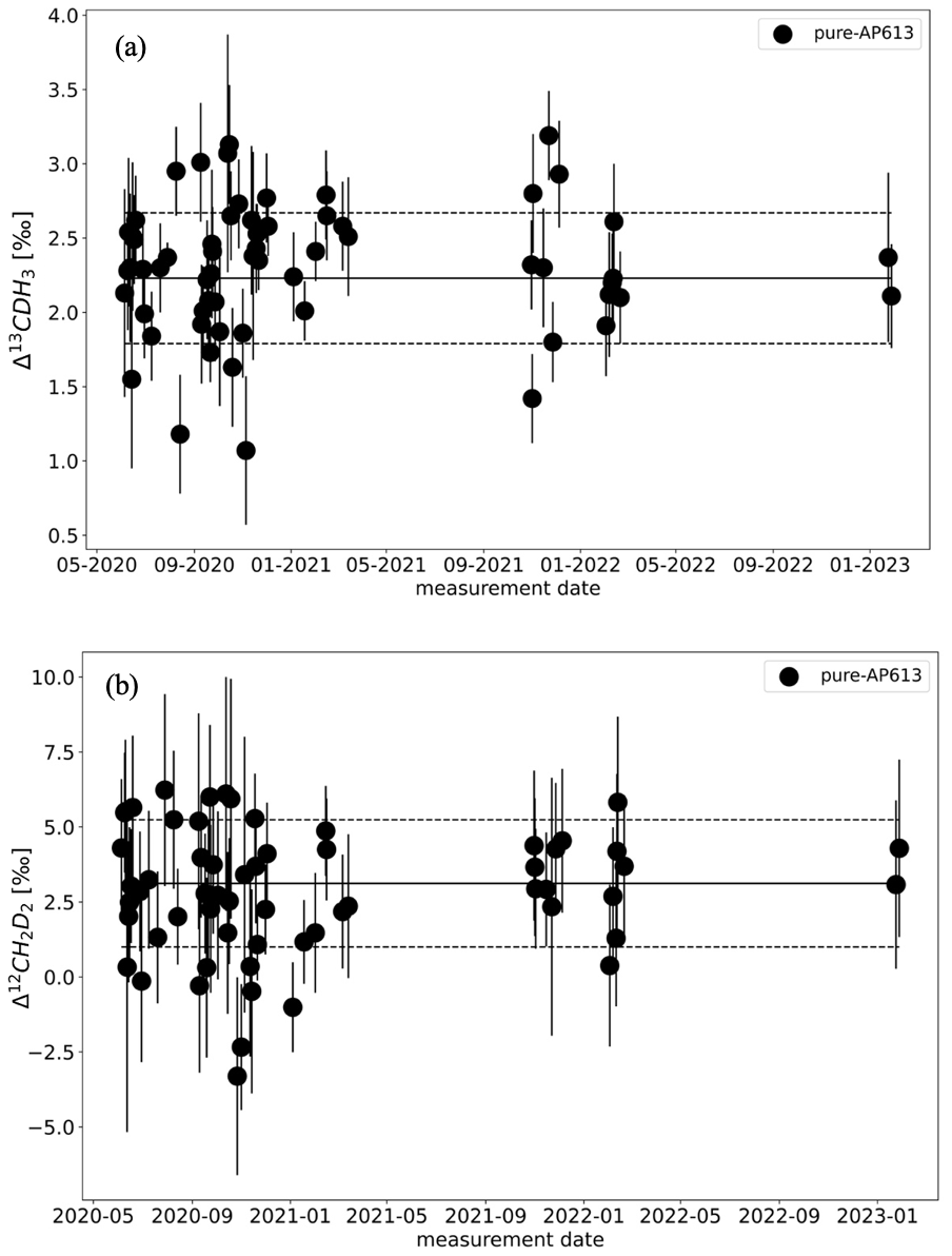
Figure 5 Results of the zero enrichment measurements, each dot representing the calculated clumping anomalies Δ¹³CDH₃ (a) and Δ¹²CD₂H₂ (b) of gas AP613. The solid black line represents the values of AP613 assigned from the temperature calibration experiments, and the dashed black lines indicate the 1σ SD of these measurements over 3 years.

The reproducibility of the measurements on the Ultra was quantified by repeated measurements of pure CAL1549 as shown in Fig. 6. Long-term reproducibility, estimated as 1σ standard deviation of the measurements of pure CAL1549 over almost 3 years, is around 0.15 ‰ for Δ¹³CDH₃ and 1.2 ‰ for Δ¹²CD₂H₂. This external reproducibility is consistent with the individual measurement uncertainty, which is on average 0.3 ‰ for Δ¹³CDH₃ and 2.3 ‰ for Δ¹²CD₂H₂ for these measurements.

Figure 6 Results of the measurements of pure CAL1549 for Δ¹³CDH₃ (a) and Δ¹²CD₂H₂ (b). The solid black line represents the average value of these measurements, and the dashed black line is the standard deviation (1σ) of the eight measurements shown.

3.4 Inter-laboratory calibration

Three of our gases (AP613, CAL1549, and IMAU-3) were measured on both the Thermo Scientific Ultra at Utrecht University (UU) and the Nu Panorama at the University of Maryland (UMD). The results of these measurements are given in Table 5.

Table 5 Comparison of Δ¹³CDH₃ and Δ¹²CD₂H₂ measurements of the three reference gases (AP613, CAL1549, and IMAU-3) on the Ultra at UU and the Panorama at UMD.

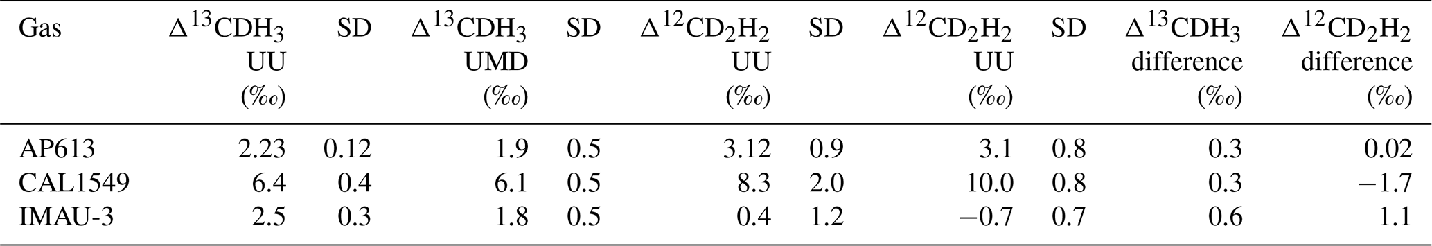
The values assigned to AP613 using our heating experiments (Sect. 3.2) agree well with the measured value of the non-heated pure AP613 on the Panorama as shown in Fig. 7. The other two gases are also within the measurement uncertainty (1σ).

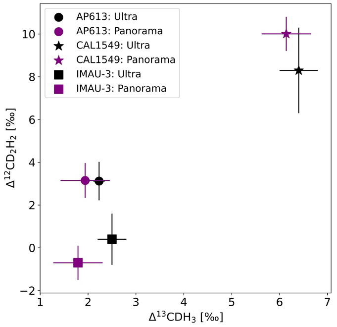
Figure 7 The clumping anomalies of AP613, CAL1549, and IMAU-3 measured on the UU-Ultra (black) and the UMD-Panorama (purple). The symbols dot, star, and square represent the gases AP613, CAL1549, and IMAU-3, respectively.

3.5 Extraction test with known gas

As mentioned earlier, mixtures of pure CH₄ from AP613 or CAL1549 with zero air were used to test and characterize the extraction system. The CH₄ extracted from these mixtures was measured against the AP613 reference gas on the Ultra. The results of the measurements are presented in Fig. 8 as the difference between the expected and the measured values. We expect this difference to be zero within the measurement uncertainty if the extraction procedure does not introduce any isotopic fractionation. Pure CH₄ from CAL1549 was also passed through the extraction system (hereby denoted as pure CAL1549 extracted) using the normal extraction procedure to check for any contamination or fractionation associated with gas introduction and collection via the extraction system.

Figure 8 Test results of the extraction system with different mixtures of laboratory reference gases as stated in the legend. Each coloured dot and star represent the difference between the measured and expected Δ¹³CDH₃ (a) and Δ¹²CD₂H₂ (b) values, respectively, of extracted-AP613 and extracted CAL1549 as given in the legend. The dashed black line is the standard deviation (1σ) of the difference for Δ¹³CDH₃ and Δ¹²CD₂H₂, respectively.

The standard deviation values of the difference between the expected and the measured values of these extraction tests are 0.4 ‰ for Δ¹³CDH₃ and 2.8 ‰ for Δ¹²CD₂H₂. Most of these extracted reference gas measurements are within this unexpected uncertainty (1σ). When the difference was more than about 2σ, additional tests were performed or parts of the system were replaced or cleaned for longer until the measurements were good enough. Typically, large offsets from the expected values are caused by incomplete trapping and releasing of gas from the silica gel used in Traps A and B of HCES. This is solved by conditioning the silica gel for longer (than the standard procedure; Sect. 2.4.1) at 150 °C.

The effect of Kr on the measurements was investigated using a 1:1 mixture of IMAU-3 and pure Kr. This mixture was directly measured on the Ultra and compared with the values of pure IMAU-3. The δ¹³C, δD, Δ¹³CDH₃, and Δ¹²CD₂H₂ values of the mixture measured on the Ultra are −34.6 ‰, −242.0 ‰, 7.45 ± 0.37 ‰, and 65.7 ± 2.3 ‰, respectively, whereas those of pure IMAU-3 are −36.6 ‰, −200.0 ‰, 2.5 ± 0.3 ‰, and 0.4 ± 1.2 ‰, respectively. This shows that Kr introduces a strong bias in the measurements of both the bulk and clumped isotopic composition of CH₄. Therefore, it is very important to remove Kr from the sample before measuring the CH₄ isotopic composition on the Ultra.

3.6 Chromatograms

Accurate and precise measurements of Δ¹³CDH₃ and Δ¹²CD₂H₂ on the Ultra require 3 ± 1 mL of pure CH₄. CH₄ from sample mixtures pre-concentrated in the extraction system is separated from the bulk sample using the GC, as explained in detail above. Chromatograms for samples with different CH₄ concentrations are illustrated in Fig. 9. When the total sample volume is above 100 mL, O₂ and N₂ are not completely separated from CH₄; therefore, a second round of GC purification is needed (Fig. 9b and c). For atmospheric CH₄ samples, separation of Kr from CH₄ is attained only when the GC columns are kept at 40 °C (Fig. 9e) instead of the usual 50 °C (Fig. 9d) used for other CH₄ samples.

Figure 9 GC chromatograms of different sample mixtures as shown in the legends. (a) Chromatogram of 20 % CH₄ +80 % zero air: 25 mL sample volume (5 mL CH₄). (b, c) Chromatograms of the first and second rounds of 1 % CH₄ + 99 % zero air: 250 mL sample volume (2.5 mL CH₄). (d) Chromatogram of a pre-concentrated atmospheric air: 70 mL sample volume (2 mL CH₄), when GC columns were heated at 50 °C and Kr is not separated from CH₄. (e) Chromatogram of pre-concentrated atmospheric air when GC columns are heated at 40 °C and Kr and CH₄ are well separated.

3.7 Propagation of error from clumping anomaly to the formation temperature

The clumping anomalies, Δ¹³CDH₃ and Δ¹²CD₂H₂, can be used to calculate the formation temperature of CH₄ when it is formed in thermodynamic equilibrium. The average precision of the Ultra measurements is 0.3 ‰ for Δ¹³CDH₃ and 2.4 ‰ for Δ¹²CD₂H₂. When propagated into the calculated temperatures (Eqs. 4a and 4b), the measurement error has a non-linear effect across the temperature range of 0 to 1000 °C. This is because of the polynomial function that defines the relation between the clumping anomalies and temperatures as given in Eqs. (4a) and (4b). Figure 10 shows that the formation temperatures can be predicted with relatively low uncertainty at lower temperatures. For example, at 50 °C the formation temperature can be estimated as ${\mathrm{50}}_{-\mathrm{12}}^{+\mathrm{13}}$ °C from Δ¹³CDH₃ and ${\mathrm{50}}_{-\mathrm{17}}^{+\mathrm{19}}$ °C from Δ¹²CD₂H₂. At 400 °C, for the same measurement precision, the temperature estimated from Δ¹³CDH₃ is ${\mathrm{400}}_{-\mathrm{66}}^{+\mathrm{90}}$ °C and from Δ¹²CD₂H₂ it is ${\mathrm{400}}_{-\mathrm{154}}^{+\mathrm{410}}$ °C. Although the absolute clumped isotope effects are larger for Δ¹²CD₂H₂ than for Δ¹³CDH₃, formation temperatures calculated from Δ¹³CDH₃ give a more precise temperature estimate because of the better measurement precision for Δ¹³CDH₃.

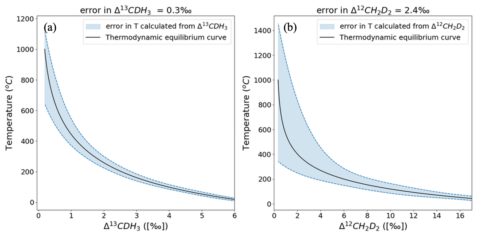
Figure 10 Error in the formation temperatures calculated from Δ¹³CDH₃ (a) and Δ¹²CD₂H₂ (b). The black solid line represents the thermodynamic equilibrium curve, and the blue dashed lines give the upper and lower limits of the errors of temperatures propagated from the errors in the measured clumping anomaly.

3.8 Overview of different samples measured

3.8.1 Samples with different source signatures

CH₄ samples collected from different origins and laboratory experiments were extracted and measured with the setup explained in Sect. 2.4. An overview of the bulk and clumped isotopic composition of some of these samples from different sources of CH₄ is presented in Fig. 11 (Table S1 in the Supplement). The precision of individual measurements is in the range of 0.2 ‰ to 0.5 ‰ for Δ¹³CDH₃ and 1.4 ‰ to 4 ‰ for Δ¹²CD₂H₂, depending on the sample volume.

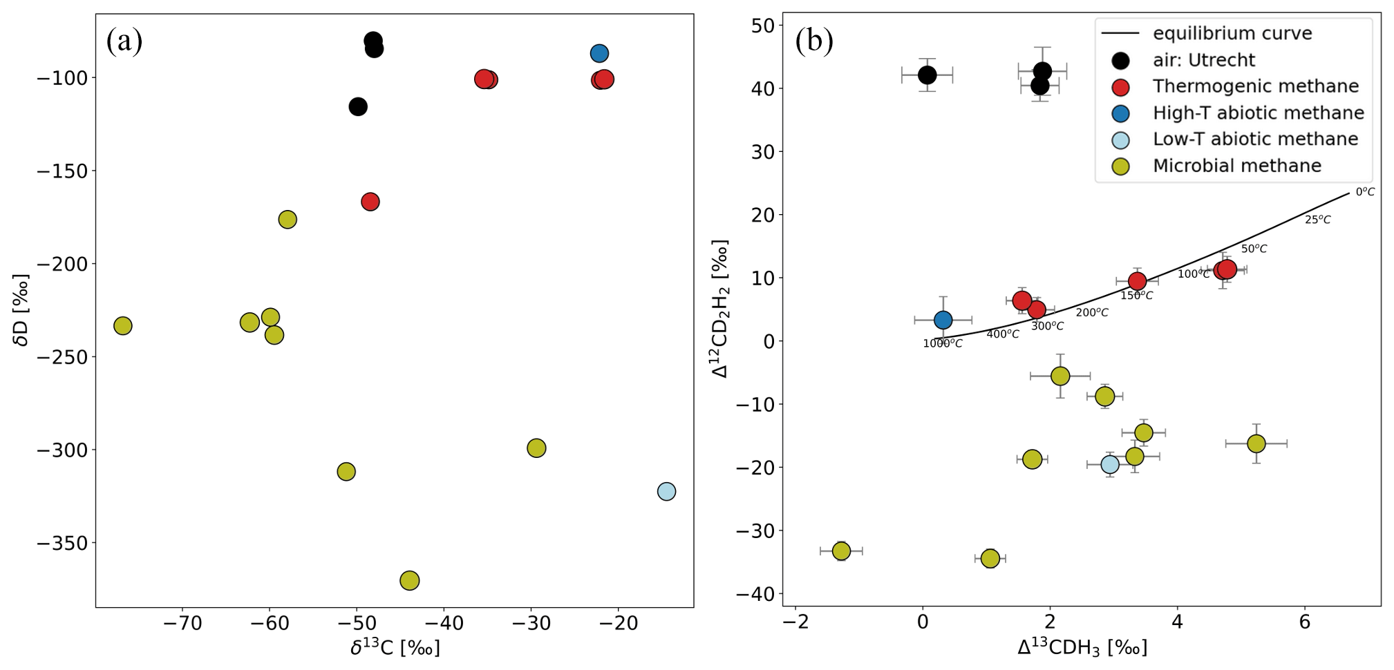
Figure 11 Comparison of δ¹³C and δD (a) and Δ¹³CDH₃ and Δ¹²CD₂H₂ (b) of samples from different source types and atmospheric air measured outside IMAU. The overview of the samples shown in this figure is given in Table S1. The solid black line represents the thermodynamic equilibrium curve with corresponding temperature values.

Most of the samples of thermogenic origin lie on or close to the thermodynamic equilibrium line; therefore, the formation temperature of CH₄ can be calculated for them. All the samples with a microbial origin (e.g. incubation experiments with methanogens, CH₄ from lake water and sediments) have depleted Δ¹²CD₂H₂ values. The low-temperature abiotic CH₄ also has negative Δ¹²CD₂H₂. This is in line with previous studies that also show that the production of CH₄ by methanogens and in rocks abiotically at lower temperatures is affected by kinetic fractionation and/or combinatorial effect that leads to negative Δ¹²CD₂H₂. So far, about 80 samples have been measured on the Ultra from very different origins with clumping anomalies ranging from −1 ‰ to 6 ‰ for Δ¹³CDH₃ and from −40 ‰ to 45 ‰ for Δ¹²CD₂H₂.

3.8.2 Ambient air measurement

Using the low-concentration extraction system (LCES), we extracted and measured several samples of atmospheric air sampled in Utrecht, and the results of the first measurements are given in Table 6.

Table 6 Results of δ¹³C, δD, Δ¹³CDH₃ and Δ¹²CD₂H₂ of atmospheric CH₄ (airs A, B, and C) sampled in Utrecht and the comparison of the measured values to the model predictions in Haghnegahdar et al. (2017) and Chung and Arnold (2021).

The solid black dots in Fig. 11b show the results of the first measurements of the clumping anomaly of atmospheric CH₄ in Utrecht (0 ‰ to 2 ‰ for Δ¹³CDH₃ and 40 ‰ to 43 ‰ for Δ¹²CD₂H₂). The air samples in Table 6 were sampled under three different atmospheric conditions: (i) clean air from the north (air A), (ii) clean air from the south (air B), and (iii) air with high CH₄ content due to local/regional pollution (air C). The values of the clumped isotopic composition of all three air samples are characterized by a very high anomaly for Δ¹²CD₂H₂ and a low anomaly for Δ¹³CDH₃. The first measurements of atmospheric methane reported by Haghnegahdar et al. (2023) of air sampled from various atmospheric scenarios in and around Maryland, USA, are compatible (0 ‰ to 3 ‰ for Δ¹³CDH₃ and 42 ‰ to 55 ‰ for Δ¹²CD₂H₂) with our measured values.

Firstly, comparing these values to the ones of CH₄ emitted from various sources, it is evident that atmospheric CH₄ has a distinct clumped signature, particularly in Δ¹²CD₂H₂. The large positive anomaly for Δ¹²CD₂H₂ of atmospheric CH₄ can be explained by a strong clumped isotope fractionation due to the sink reactions of CH₄ in the atmosphere (Haghnegahdar et al., 2017). The distinct differences between various source types and the offset of atmospheric CH₄ also suggest that more measurements of the clumping anomaly of air, especially Δ¹²CD₂H₂, can provide more information about the different sources and sink reactions that determine atmospheric CH₄ levels.

Secondly, the bulk isotopic composition (Table 6) shows as expected lower values for the polluted air C compared to the clean air A and air B, indicating regional contributions from biogenic sources as is typical for the Netherlands (Röckmann et al., 2016b; Menoud et al., 2021). However, in the case of the clumped isotopes, the air from the north is quite different in Δ¹³CDH₃, while the values for the polluted and clean air from the south are not very different, unlike the bulk isotopes. At this point we, cannot draw strong conclusions, as we only have one measurement per condition and no information on the potential variability. More measurements of Δ¹³CDH₃ and Δ¹²CD₂H₂ of air are needed to understand if short-term local/regional atmospheric changes affect the clumping anomaly of air.

Lastly, although the measured Δ¹²CD₂H₂ of atmospheric CH₄ has very high values compared to the emissions from sources, our measurement results are still far lower than recent model predictions (Chung and Arnold, 2021; Haghnegahdar et al., 2017) (Table 6). The difference can be either due to the inaccuracy in (i) source signatures of all the different sources that contribute to atmospheric CH₄ mole fraction or (ii) the theoretical values of the kinetic isotopic fractionation factor (i.e. KIE, kinetic isotopic effect) of the sink reactions of CH₄ with OH and Cl and the soil sink reactions.

We used a box model to see how the clumping anomaly of air reacts to these two parameters. The model uses clumping anomalies of the source mixture and the KIEs of OH and Cl sinks as input and gives the expected anomalies of air as output. We work with three scenarios as discussed in detail below and illustrated in Fig. 12.

Figure 12 Δ¹³CDH₃ versus Δ¹²CD₂H₂ space showing the different scenarios discussed. The solid black line represents the thermodynamic equilibrium curve. The pink dot is the value of air predicted from the source mix shown as the unfilled black circle. The solid black dot is the value of air measured on the Ultra. The three arrows show the three scenarios mentioned in the text. The dashed black circle is the new source mix calculated using scenario 3.

Scenario 1. This involves replicating the values in the study of Haghnegahdar et al. (2017). If we assume that the predicted clumping anomaly of the mixture of sources in the atmosphere (Δ¹³CDH₃=4 ‰, Δ¹²CD₂H₂=20 ‰) is accurate, then our model also gives higher values of Δ¹²CD₂H₂ and Δ¹³CDH₃ of air as in that study, with the same KIE used (OH: 1.92 for ¹²CD₂H₂, 1.33 for ¹³CDH₃; Cl: 2.2 for ¹²CD₂H₂, 1.46 for ¹³CDH₃). This was done to verify that our simple model works well for this study.

Scenario 2. This involves calculating the KIEs required to arrive at the measured values of air with the same source mix as used in Haghnegahdar et al. (2017). To get the measured values from the predicted source mix, the KIEs must be lowered to 1.79 for ¹²CD₂H₂ and 1.325 for ¹³CDH₃ for reaction with OH and 1.9 for ¹²CD₂H₂ and 1.45 for ¹³CDH₃ for reaction with Cl. This relatively small change causes a difference of about 60 ‰ in Δ¹²CD₂H₂ between scenarios 1 and 2. Therefore, the clumping anomalies are very sensitive to the KIEs of the sink reactions.

Scenario 3. This involves calculating the clumping anomaly of the source mixture that is consistent with the KIEs used in Haghnegahdar et al. (2017) and the atmospheric air measurements presented here. In this case, the clumped isotope anomaly of the source mixture must be heavily depleted, especially in Δ¹²CD₂H₂ (Δ¹³CDH₃=0 ‰, $\mathrm{\Delta }{}^{\mathrm{12}}{\mathrm{CD}}_{\mathrm{2}}{\mathrm{H}}_{\mathrm{2}}=-\mathrm{54}$ ‰), to get the measured values using the KIEs in scenario 1. This is much lower than the predicted value and would imply a strong underestimation of CH₄ sources with depleted clumping anomalies such as biogenic sources.

Given the rather high number of clumped isotope measurements of CH₄ sources that have been published to date, it seems unrealistic that the clumping anomaly of the source mix is so depleted in Δ¹²CD₂H₂ as calculated in scenario 3, which would imply that the KIE was previously indeed overestimated. These simple isotope mass balance calculations show that we need very precise estimations of the sink KIEs and more accurate measurements of the sources to completely understand the atmospheric CH₄ budget using clumping anomalies.

4 Summary and conclusion

We have presented a new versatile analytical setup for extraction, sample preparation, and measurement of the clumped isotope composition of CH₄ on the Thermo Scientific Ultra instrument, including samples at atmospheric concentration. The extraction and GC purification techniques do not cause significant isotopic fractionation and preserve the signatures of the CH₄ source. Currently, the system has been tested and works well for sample volumes of up to 1100 L. The typical precisions of samples measured on the Ultra are 0.3 ± 0.1 ‰ for Δ¹³CDH₃ and 2.4 ± 0.8 ‰ for Δ¹²CD₂H₂. The long-term reproducibility, obtained from repeated measurements of a pure methane laboratory standard over almost 3 years, is around 0.15 ‰ for Δ¹³CDH₃ and 1.2 ‰ for Δ¹²CD₂H₂. The standard deviation values of the difference between the expected and the measured values of all the extraction tests performed are 0.4 ‰ for Δ¹³CDH₃ and 2.8 ‰ for Δ¹²CD₂H₂. The total measurement time is around 20 h. The system and the measurement procedure can be adjusted to optimize the sample volume required and long measurement times. The first measurements of samples from various sources yield results in general agreement with published values. We have measured about 80 samples on the Ultra from very different origins and a wide range of clumping anomalies: −1 ‰ to 6 ‰ for Δ¹³CDH₃ and −40 ‰ to 45 ‰ for Δ¹²CD₂H₂. Our measurements of atmospheric CH₄ show enriched Δ¹²CD₂H₂ values, but they are not as high as recently predicted by clumped isotope models. It is unlikely that the discrepancy can be explained only by an underestimation of sources with negative Δ¹²CD₂H₂, but we show that a small adjustment in the KIEs of the sinks could reconcile atmospheric and source clumped isotope compositions. The precision of atmospheric CH₄ measurements can still be improved by extracting CH₄ from much larger samples (2000 L).