the Creative Commons Attribution 4.0 License.
the Creative Commons Attribution 4.0 License.
 | 17 May 2024
Mobile air quality monitoring and comparison to fixed monitoring sites for instrument performance assessment
Andrew R. Whitehill
Melissa Lunden
Brian LaFranchi
Surender Kaushik
Paul A. Solomon
Air pollution monitoring using mobile ground-based measurement platforms can provide high-quality spatiotemporal air pollution information. As mobile air quality monitoring campaigns extend to entire fleets of vehicles and integrate smaller-scale air quality sensors, it is important to address the need to assess these measurements in a scalable manner. We explore the collocation-based evaluation of air quality measurements in a mobile platform using fixed regulatory sites as a reference. We compare two approaches: a standard collocation assessment technique, in which the mobile platform is parked near the fixed regulatory site for a period of time, and an expanded approach, which uses measurements while the mobile platform is in motion in the general vicinity of the fixed regulatory site. Based on the availability of fixed-reference-site data, we focus on three pollutants (ozone, nitrogen dioxide, and nitric oxide) with distinct atmospheric lifetimes and behaviors. We compare measurements from a mobile laboratory with regulatory site measurements in Denver, CO, USA, and in the San Francisco Bay Area, CA, USA. Our 1-month Denver dataset includes both parked collocation periods near the fixed regulatory sites and general driving patterns around the sites, allowing a direct comparison of the parked and mobile collocation techniques on the same dataset. We show that the mobile collocation approach produces similar performance statistics, including coefficients of determination and mean bias errors, to the standard parked collocation technique. This is particularly true when the comparisons are restricted to specific road types, with residential streets showing the closest agreement and highways showing the largest differences. We extend our analysis to a larger (yearlong) dataset in California, where we explore the relationships between the mobile measurements and the fixed reference sites on a larger scale. We show that using a 40 h running median converges to within ±4 ppbv of the fixed reference site for nitrogen dioxide and ozone and up to about 8 ppbv for nitric oxide. We propose that this agreement can be leveraged to assess instrument performance over time during large-scale mobile monitoring campaigns. We demonstrate an example of how such relationships can be employed during large-scale monitoring campaigns using small sensors to identify potential measurement biases.
- Article
(9916 KB) - Full-text XML
-
Supplement
(2466 KB) - BibTeX
- EndNote


Mobile air pollution monitoring can resolve fine-scale spatial variability in air pollutant concentrations, allowing communities to map air quality down to the scale of tens of meters in a reproducible manner (Apte et al., 2017; Van Poppel et al., 2013). Expanding fleet-based mobile monitoring will allow the mapping of much larger spatial regions over longer periods and with more repetition. This will improve the accuracy of land use regression models (Messier et al., 2018; Weissert et al., 2020) and supplement our understanding of air quality issues in environmental justice regions (Chambliss et al., 2021). One concern with fleet-based mobile monitoring, especially as it expands to lower-cost and lower-powered instrumentation, is maintaining instrument performance (accuracy, precision, and bias) over time in a mobile environment. While the use of fleets facilitates the scaling of mobile monitoring to large geographic scales, such as multiple counties in an urban area or multiple cities across a large state, coordinating vehicles and drivers across these geographies makes laboratory-based calibrations costly, time-consuming, and impractical. Moreover, instrumentation can behave differently in a field environment compared with during laboratory testing and calibration (Collier-Oxandale et al., 2020), making field calibrations or collocations essential for quantitative measurement applications. Field validation usually involves the collocation of one or more test instruments with reference-grade instruments at a fixed monitoring site, such as a regulatory site (Li et al., 2022). Frequent collocations with fixed reference sites have been identified as an important component of quality assurance for mobile monitoring campaigns (Alas et al., 2019; Solomon et al., 2020). Collocated measurements within ongoing campaigns can also be used to identify potential measurement issues. For example, Alas et al. (2019) provide an example of how the collocation of two AE51 black carbon monitors was used to identify and correct unit-to-unit discrepancies during an ongoing mobile monitoring campaign. Collocated measurements are also important for the validation of other emerging measurement technologies, such as lower-cost sensors (Bauerová et al., 2020; Castell et al., 2017; Masey et al., 2018).
For mobile monitoring applications, parking a mobile platform next to a fixed reference site approximates the collocation technique for assessing instrument performance. Collocated parking can be incorporated into driving patterns for large-scale mobile monitoring campaigns. However, parking near a fixed reference site ensures comparability only at that specific location and only under the specific atmospheric conditions over which the collocation occurred. As a result, many repeat collocations must be performed, leading to inefficiencies in data collection and an approach that is not easily scalable to larger mobile monitoring campaigns. In addition, natural spatial variability in pollutant concentrations makes the selection of collocation site important (Alas et al., 2019; Solomon et al., 2020), which can often prove restrictive for extended monitoring campaigns. In addition, strong agreement between measurements when collocated at a fixed reference site may not translate directly into accuracy and precision in other environments (e.g., Castell et al., 2017; Clements et al., 2017).
Ongoing mobile (“in motion”) comparisons with fixed reference sites are more scalable than frequent side-by-side parked collocations and could provide an important tool for ongoing instrument performance assessments during extended mobile monitoring campaigns. If collocation comparisons can be extended out to kilometer scales and spread across multiple fixed reference sites over the course of a single campaign, the number of data used to evaluate the mobile measurements will be increased, the dynamic range of the pollutant concentrations being measured will be larger, and more time can be dedicated to meeting the mobile monitoring data objectives. In this study, we compare mobile air pollution measurements to fixed-reference-site measurements from both parked and mobile collocations during the same campaign. The objective is to determine if changes in instrument performance, such as bias, can be identified in mobile collocations to a similar degree to those from stationary collocations. We will look at using mobile–fixed site comparisons as a function of road type and distance between the vehicle and the fixed reference site and compare them to the parked comparisons.
If mobile collocation is able to quantitatively assess bias in mobile instrumentation, it would allow easier detection of instrumental drift over time or sudden changes in instrument performance that could indicate a malfunction. This methodology will not serve as a calibration of the mobile platform or replace traditional calibration and quality assurance techniques; rather, it is meant to supplement traditional techniques to allow earlier identification of measurement issues during ongoing mobile monitoring campaigns. We explore the concept of mobile collocations using fast-response (1 or 0.5 Hz), laboratory-grade air pollution monitoring instrumentation which is independently calibrated and subject to strict quality assurance. This allows us to explore the impact of spatial variability in pollutant concentrations and operational differences in the mobile–fixed site comparisons without being limited by instrument accuracy or precision concerns. This will help us to understand the strengths and limitations of these methods and to quantify the magnitude of biases that could be detected using these methods. This work could be expanded in the future to midrange instrumentation and smaller-scale sensors of various pollutants and further developed into a scalable approach for ongoing instrument performance assessment during fleet-based mobile monitoring campaigns where frequent in situ calibrations of sensors using traditional methods is not feasible.
For this study, we focus on the pollutants ozone (O3), nitrogen dioxide (NO2), and nitric oxide (NO). This decision is largely based on the availability of both mobile and fixed-reference-site data for the two studies that we analyze. O3 and NO2 are “criteria” pollutants with adverse health effects that are measured and regulated by the United States Environmental Protection Agency (US EPA), and all three species are commonly measured at air quality monitoring sites in the USA and other countries. The data collected in this study come from two mobile monitoring deployments: one in Denver, CO, USA, in 2014 and one in the San Francisco Bay Area, CA, USA, in 2019–2020. The first study included both parked and mobile collocations and allows a direct comparison of the two techniques, whereas the second study contains a larger dataset that permits a deeper exploration of the relationship between distance and temporal aggregation scales for optimizing the comparisons. We also demonstrate a real-world application of the method to detect drift in an NO2 sensor deployed as part of Aclima's collection fleet. Finally, we discuss the results within the context of the spatial heterogeneity of the observed pollutants and the implications for extending the approach to additional pollutants not included in this study.
We analyze measurements from several different vehicles equipped with an Aclima mobile laboratory measurement and acquisition platform (Aclima Inc., San Francisco, CA, USA). These measurements come from two separate deployments at different locations and during different time periods. For the first deployment, three Google Street View (gasoline-powered Subaru Impreza) cars were outfitted with the Aclima platform in Denver, CO, USA, during the summer of 2014 (Whitehill et al., 2020). The second set of data comes from Aclima's Mobile Calibration Laboratory (AMCL), a gasoline-powered Ford Transit van that we deployed in the San Francisco Bay Area of California in 2019–2020. Aclima designed the AMCL to support the field calibration of their sensor-based Mobile Node (AMN) devices for deployment in the Aclima mobile monitoring fleet. In both studies, the mobile platforms were equipped with high-resolution (0.5 or 1 Hz data reporting rate), reference-grade air pollution instrumentation to measure O3, NO2, and NO. Additional measurements, including black carbon (BC), size-fractionated particle number (PN) counts, and other species were also measured during these campaigns but are not discussed in this publication. For this paper, we focus on measurements that had equivalent mobile and fixed-reference-site measurements for both studies. A critical part of this work is our comparison of parked and mobile collocations during the 2014 Denver study, for which we had 1 min averaged reference site data for O3, NO2, and NO but not the other measured species.
O3 was measured using ultraviolet (UV) absorption with a gas-phase (nitric oxide) O3 scrubber for the ozone-free channel (Model 211, 2B Technologies). This technology reduces some of the volatile organic compound (VOC) interferences observed in other UV photometric ozone monitors (Long et al., 2021) and has been designated as a federal equivalent method (FEM) by US EPA (2014). The 2B Model 211 only reports ozone at 2 s intervals, so ozone was measured and reported as 2 s averages for the Denver study. For the California study, all ozone data were averaged up to 10 s averages during initial data collection, so 10 s averaged data are used for the analysis. NO2 was measured using cavity attenuated phase shift (Model T500U, Teledyne API) and represents a “true NO2” measurement (Kebabian et al., 2005). The Teledyne API Model T500U has been designated as an FEM by US EPA (2014). NO was measured using O3 chemiluminescence (CLD 64, Eco Physics), which is a recognized international standard reference method for measuring NO (e.g., EN 14211:2012). NO and NO2 are both measured as 1 s averages in both studies. These instruments have all been evaluated by strict test criteria and are recognized as reference methods by various regulatory agencies; however, the reference method designations do not apply to the applications (mobile monitoring) and timescales (1 s to 1 h) assessed here. These instruments were chosen for their demonstrated excellent data quality and performance to serve as a mobile reference for calibration purposes. It is important that we assess these methods using reference-grade equipment so we can focus on variability due to spatial heterogeneity instead of instrument issues. If the methods that we develop here are successful with reference-grade equipment, they can be used to evaluate the performance of low-cost sensors, which might not meet the same strict regulatory standards at present but can still provide valuable data in smaller, lower-power, and lower-cost form factors (Castell et al., 2017; Clements et al., 2017; Wang et al., 2021).
3.1 Methods
We begin the analysis with the comparison of measurements from a parked mobile platform to those at a nearby fixed reference site. For this analysis, we use data from a mobile measurement campaign that occurred in Denver, CO, USA, during the summer of 2014. Professional drivers drove three identical mobile air pollution monitoring platforms, consisting of specially equipped Google Street View cars, through the Denver, CO, greater metropolitan region between 25 July 2014 and 14 August 2014. The project goals were to evaluate the performance of the mobile monitoring platforms and to develop methods for assessing data quality and platform comparability. The three cars drove coordinated routes in a 5 km area around several regulatory monitoring sites in the Denver, CO, area as well as driving around larger (10 km) areas to understand the variability in air pollutants at different spatial scales. At several planned periods during the study, the drivers were instructed to park one or more of the cars near one of the fixed regulatory monitoring sites in the region. These parked collocations were integrated into the experimental plan to facilitate the assessment of the data quality of the mobile platform by comparison to fixed-reference-site measurements. The parked collocations lasted about 20 min each and included comparisons at the Colorado Department of Public Health and Environment (CDPHE) CAMP (39.751184° N, 104.987625° W) and La Casa (39.779460° N, 105.005124° W) sites. The drivers were instructed to park as close as possible to the site but were required to park in an available public parking space on a public street. These restrictions limited how close each car could get to the reference site for each collocation and resulted in individual parked collocation locations ranging in distance from the regulatory stations, as shown in Fig. 1. In addition, the drivers were instructed to park facing into the wind when possible to minimize the influence of self-sampling, which posed additional restrictions. A visual screening did not reveal any suspected self-sampling periods, so no additional attempts were made to identify or remove such periods. Additional details about the monitoring campaign can be found in the Supplement and in Whitehill et al. (2020). The CDPHE reported hourly federal reference method (FRM) and FEM measurements of O3, NO2, and NO, and also reported 1 min time resolution data for our study period as part of the 2014 DISCOVER-AQ field campaign (https://www-air.larc.nasa.gov/missions/discover-aq/discover-aq.html, last access: 9 May 2024).
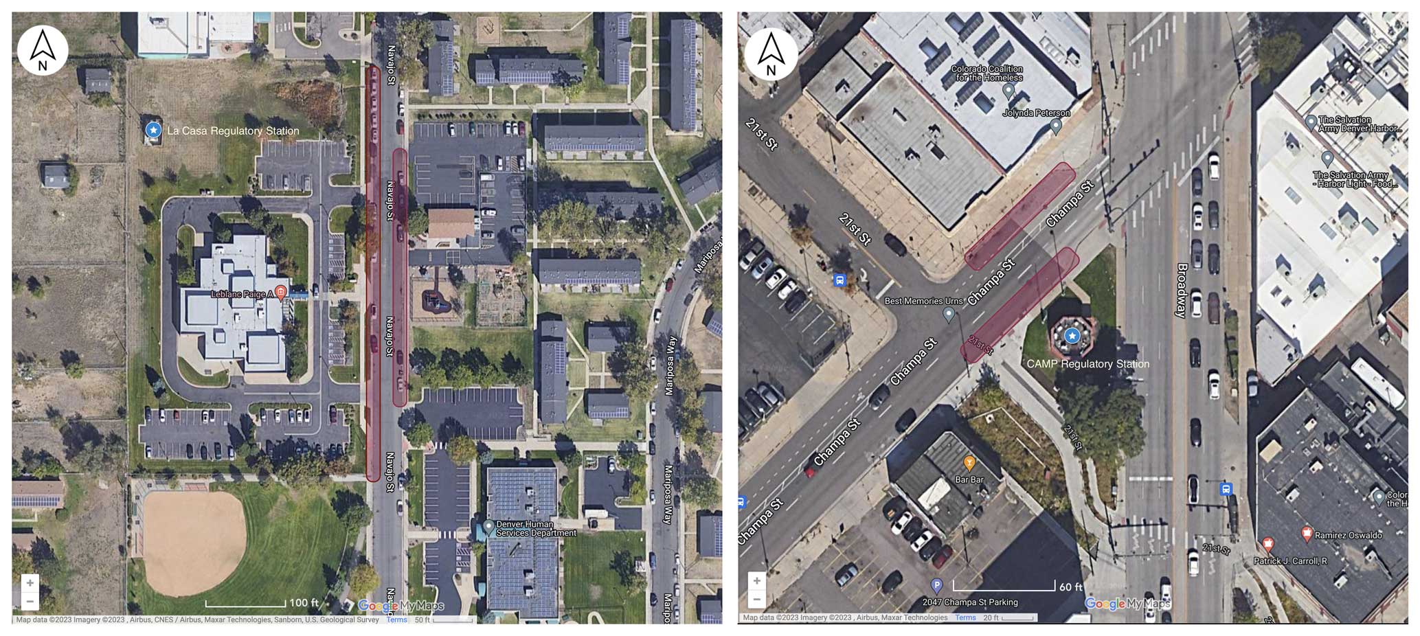
Figure 1Satellite view of the area in the immediate vicinity of the La Casa (left) and CAMP (right) regulatory sites. The blue markers denote the regulatory sites and the red shaded areas indicate the range of areas where the vehicles parked during most of the parked collocation periods. Car-to-site distances varied from 80 to 145 m for the La Casa site and from 10 to 85 m for the CAMP site. (Not shown are two periods during which the cars parked at the CAMP site just north of the map due to a lack of street parking closer to the site).
Aclima staff performed quality assurance evaluations on the instruments daily in the field and after the study in the Aclima laboratory. Flow rates remained within instrument specifications throughout the study. We used instrument responses to zero air (from a zero-air cylinder) to apply a study-wide zero offset for each instrument on each car. Results from daily span checks for NO (360 ppbv) and O3 (80 ppbv) did not drift beyond the instruments' specifications during the study, so no adjustments were made to instrument span values during the study. All calibrations were performed “through the probe” by connecting a dilution gas calibrator to the sample inlet in a vented tee configuration. A certified NO gas cylinder was diluted by zero air to provide a 360 ppbv NO span gas for the NO instrument, and a certified O3 generator was used to produce 80 ppbv O3 for the O3 span checks. We calibrated the NO2 instrument before and after the study in a laboratory but only performed zero checks on the NO2 instruments in the field.
The bias of the O3 instruments varied between 3 % and 6 % with a standard deviation of 5 %. The bias of the NO instruments varied between 3 % and 8 % with a standard deviation of 6 %. Field bias measurements are based on span checks assuming the linearity of the instrumentation response across the measurement range, which was confirmed in laboratory multipoint calibrations. At the mean observed concentrations during the study (33 ppbv O3 and 53 ppbv NO), the error in span measurements translates to an average bias and precision of 2 ppbv for O3 and an average bias and precision of less than 4 ppbv for NO. The NO standard gas had a concentration uncertainty of ±2 % (EPA protocol gas grade). Mass flow controllers in the dilution calibrator were within their certification period and had a specified accuracy of ±3.6 % at the conditions used to generate the span gases. The accuracy of the O3 generator was ±1 % and was certified less than 3 months before the study. We attempted to perform gas-phase titration to produce NO2 span gases in the field, but technical issues prevented us from performing accurate daily span checks on NO2. We did not observe any drift in the NO2 instruments between the pre-campaign calibration and the post-campaign calibration of the NO2 instruments, so we assumed the calibration of the NO2 instrumentation was constant throughout the campaign period.
At least one of the cars was parked at the CAMP site (within 85 m) for 15 time periods during the study (Table S1 in the Supplement) and at the La Casa site (within 150 m) for 16 time periods (Table S2 in the Supplement). We previously compared measurements among the three equivalently equipped cars (Whitehill et al., 2020) and determined that 1 s NO2 and O3 measurements agreed to within 20 % during a day of collocated driving. NO measurements showed higher variability, likely reflecting hyperlocal differences in NO concentrations from exhaust plumes, but were still within 20 % about one-third of the time. A similar comparison of two Aclima-equipped Google Street View cars in San Francisco and Los Angeles also showed excellent car-versus-car comparability (Solomon et al., 2020). For the purposes of the present analysis, we assume that the data from the three cars are equivalent and interchangeable.
We aggregated all the data up to 1 min averages (using a mean aggregating function) to put the car measurements on the same timescale as the 1 min DISCOVER-AQ measurements reported by CDPHE for the CAMP and La Casa sites.
3.2 Results and discussion
Figure 2 shows scatterplots comparing 1 min O3, NO2, NO, and OX (O3+NO2) for the parked cars versus the fixed reference sites (black circles); it also displays the period-specific mean data (yellow circles) and the one-to-one (1:1) line (dashed line). OX was included in the analysis because it is more likely to be conserved in fresh NOX emission plumes (assuming most of the NOX is emitted as NO) than O3 or NO2 separately. We calculated the period-specific means by averaging the discrete 1 min measurements over the continuous measurement periods that the cars were parked at the fixed reference site (Tables S1, S2). We also calculated period-specific medians in a similar way and computed ordinary least-squares (OLS) regression statistics for the 1 min data, the period-specific means, and the period-specific medians (Table S3 in the Supplement).
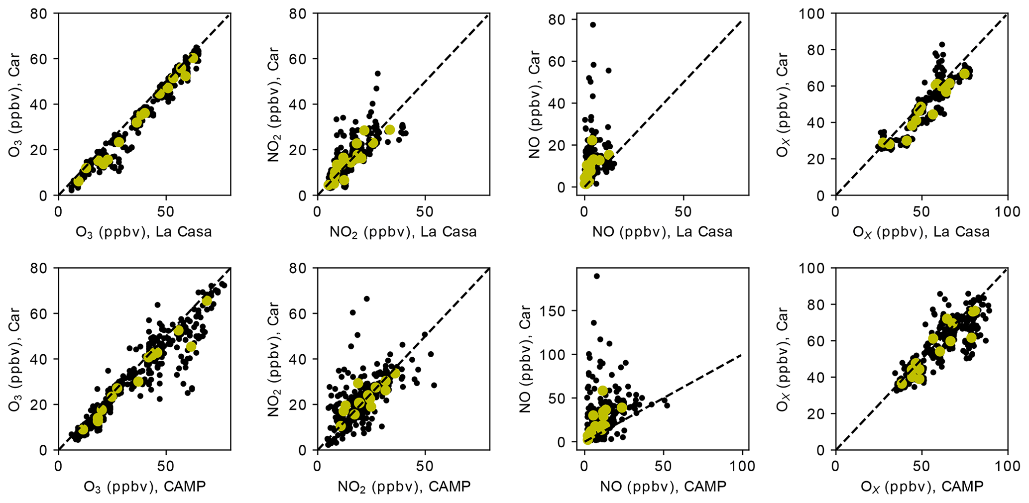
Figure 2Scatterplots of 1 min (black dots) and period mean (yellow dots) car measurements (O3, NO2, NO, and OX) versus fixed-reference-site (La Casa or CAMP) measurements during the stationary collocation periods. A black dashed 1:1 line is provided for reference.
Figure 2 shows relatively good agreement in the 1 min observations between parked mobile and stationary reference measurements of O3 and NO2 (and OX), despite some scatter in the relationship. The agreement for NO is poor relative to that for the other pollutants. The coefficient of determination (r2) values are highest (in descending order) for O3, NO2, and NO (see Table S3). With the exception of O3, the linear regression statistics, such as slope and intercept, did not provide an accurate assessment of bias due to the influence of outlier points on the OLS regression statistics, as evidenced by the relatively low r2 (for NO2 and NO in particular). This relationship is consistent with the expected trends in spatial heterogeneity between the three pollutants (Sect. 7) and illustrates how there can be significant variability in the 1 min differences between parked mobile and stationary measurements. The r2 does improve somewhat when using the period-specific aggregates (mean and median; Table S3), suggesting that temporal aggregation can reduce some of the variability in the difference and improve the comparisons.
In order to minimize the impact of scatter in the measurements further, we also looked at the statistics of 1 min mobile–fixed-site differences, here denoted as . We looked at the mean (i.e., mean bias error), median, standard deviation, and 25th and 75th percentiles of the ΔX distributions (Table 1). The mean and median of the ΔX values effectively aggregate the observations across all of the parked collocation periods and are a more direct assessment of systematic offset bias than the slope and intercept of the OLS regressions (especially for NO2 and NO). This is due to the high sensitivity of the OLS regression statistics to outlier points. Given that the measurements are made under nonideal conditions, such as the on-the-road, parked (nearby but not spatially coincident) collocations where spatial variability in pollutant concentrations at fine spatial scales appears to be significant, a few extreme outlier points might occur that will skew the OLS statistics but will have less influence on the ΔX statistics. For the ease of discussion, in this and subsequent sections, we refer to these ΔX values generally as “bias”, which includes both spatial and measurement bias.
Table 1Statistics of 1 min ΔX comparisons for the stationary collocated periods. Units are parts per billion by volume (ppbv). SD is standard deviation, P25 is the 25th percentile, and P75 is the 75th percentile.
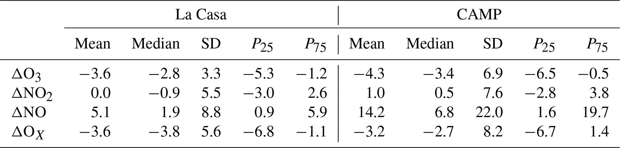
From Table 1, NO2 shows excellent agreement between the mobile platforms and the fixed reference sites. Mean and median bias values for NO2 were within 1.0 ppbv of 0 for both the CAMP and La Casa sites. O3 shows a minor (but persistent) offset of around 3 ppbv for both sites, which is also apparent from the scatterplots (Fig. 2). Both the 25th and 75th percentiles for ΔO3 were negative as well, suggesting a real differences in the ozone measurements between the mobile platform and the fixed reference site. The OX biases were similar to the sum of those for O3 and NO2, as anticipated from our definition of OX. Although the median NO bias for the La Casa site was small (1.9 ppbv), the mean bias for the La Casa site and the mean and median biases from the CAMP site were significantly larger, with values between 5.1 ppbv (for the La Casa mean) and 14.2 ppbv (for the CAMP mean).
The La Casa site is located over 80 m from the nearest street in a predominantly residential neighborhood (Fig. 1). The CAMP site, in contrast, is located within meters of the intersection of two major roads (Broadway and Champa St.) and is surrounded by commercial properties. The influence of concentrated direct emission plumes at the mobile platform are a primary source of discrepancies between the mobile platform and the fixed reference site. The relative biases in instrument calibration and differences in concentrations due to the relative proximity of the two instruments to passing emission plumes may also contribute to the discrepancy. From the combined time series of all collocations (Figs. S4 and S5 in the Supplement), short-term peaks in NO and NO2 are present in the mobile-platform measurements but not in the fixed-reference-site measurements. This reflects the impact of emission plumes from local traffic. The traffic influences are particularly noticeable at the CAMP site, reflecting its location at a major intersection. While we cannot rule out self-sampling of exhaust from the mobile platform, the higher frequency of plume events at the CAMP site compared with the La Casa site suggests that local traffic emissions are the primary source of the observed pollution plumes.
The parked collocation results support the assessment of instrument bias; however, the influence of local traffic emissions on the collocation does result in nonoptimal conditions. Temporal aggregation can smooth some of the outlier points and make the results more reflective of real measurement differences; nevertheless, parametric regression statistics will still be biased by the influence of outlier points. Although it is possible to impose strict collocation criteria for parked collocations that would limit the influence of local emissions, the operational constraints during large-scale mobile monitoring campaigns often necessitate the use of publicly accessible sites for frequent collocations. As most scalable parked collocation solutions are likely to be affected by traffic emissions, expanding to allow the use of additional data while driving in the vicinity of the fixed reference station should be explored as a viable alternative. Mobile collocations have the added advantages that spatial biases are averaged out by the motion of the mobile platform through space, effectively allowing each mobile data point to sample a larger (and, by extension, more representative) amount of air in the same sampling duration (e.g., Whitehill et al., 2020). For example, a car traveling 25 m s−1 will “sweep” an additional area of 1500 linear meters in 1 min compared with the stationary sampling. Thus, regardless of the wind speed, a moving platform will integrate each measurement over a larger area than a stationary platform, making each emission point source have less direct influence on the entire integrated measurement.
4.1 Methods
To assess the performance of a mobile collocation approach, we used all the measurements (stationary and moving) collected during the 2014 Denver study, employing the parked collocation results as a point of reference. We associated the raw 1 Hz car data with the nearest road using a modified “snapping” procedure (Apte et al., 2017); utilizing the aforementioned procedure, we associated each mobile data point with the nearest road segment whose direction was within 45° of the car's heading. We assigned each 1 Hz data point to one of four different road types (“Residential”, “Major”, “Highway”, or “Other”) based on the OpenStreetMap (OSM) road classifications of the nearest road segment identified during the snapping procedure (Table S4 in the Supplement). We also created an aggregate “Non-Highway” road class, which consisted of roads in the Residential, Major, and Other road classes (i.e., everything not classified as a Highway). Based on our results from Sect. 3, we believe that the measurements made on Residential roads will generally have lower traffic, and thus stronger agreement with measurements at most fixed reference sites. While traveling on high-traffic roads (such as highways), the cars are more likely to be impacted by direct emission plumes. In effect, we are assuming that the OSM road classifications is a general proxy for the on-road traffic volume. In addition to road type, we anticipate that the distance between the fixed reference site and the mobile platform will affect the comparisons, with the closest agreement when the distances are small. Although more sophisticated methods are possible to identify and remove high-traffic roads, OSM road classifications are a general proxy that can be applied algorithmically over a large portion of the Earth. In contrast, local traffic count data are more sporadic and not always available or easily accessible for the region of interest.
We looked at the mean and median biases and coefficients of determination for measurements made by the cars versus those at the La Casa site. We broke down the analysis by road class and distance buffer, starting at a distance buffer of 500 m and expanding out in 250 m increments. Our goal was to explore how the central tendency of the bias distribution was affected by the cars' distance from the La Casa site as well as by the impact of different road types. We also present (in the Supplement) scatterplots and linear regression statistics for five discrete buffer distances (100, 300, 1000, 3000, and 10 000 m) and the five different road classes.
4.2 Results and discussion
There are fundamental differences between the in-motion collocations discussed in this section and the parked collocations discussed in Sect. 3. These differences have implications for the interpretations of central tendency (mean or median) bias values and r2 values. In general, the mean and median bias values from both stationary and in-motion collocations can reflect both measurement bias as well as persistent spatial differences, especially when the instrument inlets are not located at the exact same location. The r2 values generally reflect the variability between the mobile and stationary measurements that results from a combination of measurement precision as well as true spatiotemporal variability. Spatiotemporal variability, in this context, refers to differences in space at the same instant in time, rather than spatial differences that persist over time and are apparent with aggregation over time, which we refer to as systematic spatial bias. At any given instant, the differences between mobile and stationary measurements of different air parcels in different locations are effectively random due to variability in wind direction, wind speed, atmospheric turbulence, and emission rates, among other factors. These factors influence the collection of comparison data points for use in the estimate of r2. For the in-motion observations, both the bias values and the r2 values reflect additional sources of spatial variability that need to be considered compared with the parked collocations. This is due to the wider range of distances (up to 5 km), varying road types and associated traffic patterns, and potentially different spatial distributions of nonmobile sources in the wider areas covered. As discussed in Sect. 3, r2 values vary depending on the pollutant measured and can be quite low, even for parked collocations. As a result, we conclude that r2 would not be a good indicator of instrument performance (i.e., precision error) and that using a parametric linear model to attribute gain and offset instrument biases separately is not possible, particularly for NO and NO2. Therefore, the inclusion of r2 in this section is primarily as context for understanding random spatiotemporal variability (as described above) in the comparisons. The focus of this section is to characterize the dimensions over which these spatiotemporal differences, both random and systematic, manifest in the data. By doing so, we hypothesize that we will be able to isolate the conditions under which the variability in bias values can be expected to reflect variability in measurement bias between the mobile and stationary monitors. In particular, we are looking for an optimal operational method for mobile collocation that provides comparable results to that determined from the parked collocations.
The mean and median bias values and r2 values for the car–La Casa comparisons are shown as a function of buffer distance and road type in Fig. 3. Note here that, for each distance D, we include all data points within a distance of D from the stationary site, so we are not explicitly showing how bias varies with distance from the stationary monitors. We also display the results from the stationary collocation analysis (Sect. 3) to demonstrate the similarity between the mean and median biases and r2 values from the stationary collocations alongside those from our expanded analysis in this section. Because measurement bias is not expected to correlate with the spatial dimensions featured in these analyses, the difference between road types and with varying distances from the site can be interpreted purely as persistent spatial differences. As shown in Fig. 3, measurements from the Highway road class resulted in a significantly higher magnitude of bias compared with other road types, indicating a larger influence of direct emission plumes increasing the variability in concentrations measured on Highways (with respect to the stationary-site measurements) than for other road types. The r2 values on Highways are generally lower than on other road types, indicating that there is higher random variability on Highways compared with the stationary-site measurements. Differences in bias and r2 between Major and Residential road types are significant in some cases and less so in others, depending upon the pollutant and the distance. However, even in cases where the differences are significant (e.g., NO2 at distances greater than 1000 m), the magnitude of the bias for Major roads is only a fraction of that from Highways. As discussed above, the degree of bias and random spatial variability between the mobile measurements and the fixed reference sites are primarily impacted by the direct emission plumes on the roadway. We anticipate that Highways have higher traffic and a higher fraction of more heavily polluting vehicles (e.g., heavy-duty trucks), which explains the larger magnitude of bias and lower r2 values. Roads with lower expected traffic volumes and less heavy-duty vehicles, such as Residential roads, have a lower magnitude of bias.
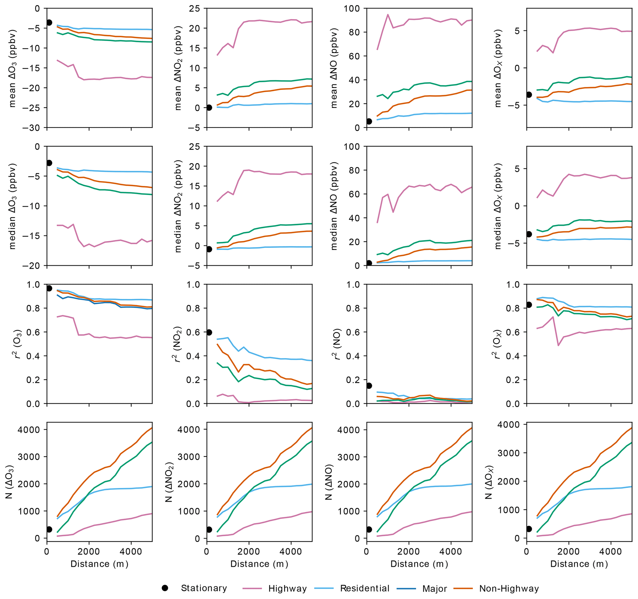
Figure 3Mean and median ΔX, coefficient of determination (r2), and number of data points (N) for 1 min car–La Casa comparisons as a function of the maximum distance between the car and the La Casa site. Results from stationary collocations (Sect. 3) are shown as black dots, whereas different road classes are shown using different colors.
For all road types, the bias between the mobile measurements and the reference site is lowest (and r2 is highest) for distance buffers closest to the site. For the Residential road class, the bias between mobile collocation and parked collocation changes very little as the distance buffer increases for all species. The bias for observations collected on Major and Highway road types generally increases as additional samples are included at greater distances from the site.
When considering the results of bias by road type and distance class, it is important to note that the distribution of road type varies by distance. This is indicated by the number of data points (N) by road type as a function of distance in Fig. 3. The La Casa site is in a residential area, so most of the roads within 500 m of the site are Residential. The designated drive patterns near the La Casa site resulted in most of the mapped roads within 2 km of the site being a combination of Residential and Major road types. Further away from the La Casa site, the roads consisted of a larger fraction of Major roads and Highways that were used to commute between the different areas where the denser mapping occurred.
For both Major and Residential road types, the bias and r2 values tend towards the values from the parked collocations as the buffer distance decreases in most cases. Note that most of the mobile-to-stationary data within 1 km of the La Casa site were measured on the same days and generally within a 2 h window of the stationary collocation data. For NO and NO2, there are some slight differences between the parked collocation results and the 500 m buffer distance, with slightly higher bias on Major roads compared with the parked collocations. For NO and NO2, this indicates an increase in the systematic spatial bias when in motion on nearby Major roads compared with when parked as well as minimal differences in random variability. These results highlight the potential of in-motion mobile collocation compared with parked collocations in reducing the random variability, especially on Residential roads in the immediate vicinity of the stationary site. In general, however, there is remarkable consistency between the in-motion and parked collocation results for all pollutants when Highways are removed from the dataset. Depending upon the target quality assurance guidelines of the study, there might be significant advantages to using in-motion mobile collocations instead of parked collocations to determine changes in mobile versus stationary measurement biases.
Scatterplots of the 1 min mobile-platform measurements versus the 1 min La Casa measurements are shown in the Supplement for O3 (Fig. S6), NO2 (Fig. S7), NO (Fig. S8), and OX (Fig. S9). These are shown, along with OLS linear regression statistics, for each individual road class and for distance buffers of 100, 300, 1000, 3000, and 10 000 m. As with the stationary collocation scatterplots (Fig. 2), these show the best agreement (i.e., closest to the 1:1 line) for O3 and OX, with moderate agreement for NO2 and the worst agreement for NO. As suggested above, the regression statistics (slope and intercept) appear to be a poor indicator of agreement, especially for directly emitted species like NO (and, to a lesser degree, NO2). Therefore, we focus our analysis on the central tendency metrics of the bias and the r2 values, as shown in Fig. 3.
One final consideration for interpreting the impact of spatial variability in the Denver dataset is the impact of temporal aggregation. The availability of data from a fixed reference site at 1 min time resolution was unique to the experimental study in Denver, with additional instrumentation added to support the research objectives of the 2014 DISCOVER-AQ experiment. Data from regulatory monitoring stations in the USA are typically only available at 1 h time resolutions, and these are the data that we had available for the California dataset in Sect. 5. For mobile collocations to be broadly applicable to large-scale mobile monitoring applications, it is important to assess how the results change when the mobile data are compared with 1 h stationary data. We averaged the mobile data by taking the mean of 1 s measurements within each hour-long period that fit the appropriate road type and buffer distance criteria. Figure 4 compares the results of the 1 h aggregated comparisons to the 1 min comparisons as a function of buffer distance for the Non-Highway road class. Generally, the results for the 1 min and 1 h aggregation are similar in terms of both bias and r2. For O3 and OX, the differences are minor. For NO2 and NO there is a slight increase in the median bias as well as an increase in r2 for the 1 h comparisons versus the 1 min comparisons. The r2 at 1 h for NO2 and NO is variable as a function of the distance buffer, likely due to the limited size of the dataset and the variable distribution of road type with distance, so this may not be an accurate assessment. The increases in r2 for NO2 and NO suggest that there is a modest reduction in the impact of random spatial variability at hourly aggregations; however, the increase in bias suggests that there is additional apparent bias as a result of the aggregation. This could be due to the incomplete hourly aggregates from the mobile platform being compared to the full hourly observations from the stationary site. However, the Denver dataset is too limited to explore this hypothesis adequately. The number of data points per hourly mobile collocation will be explored more thoroughly in Sect. 6.
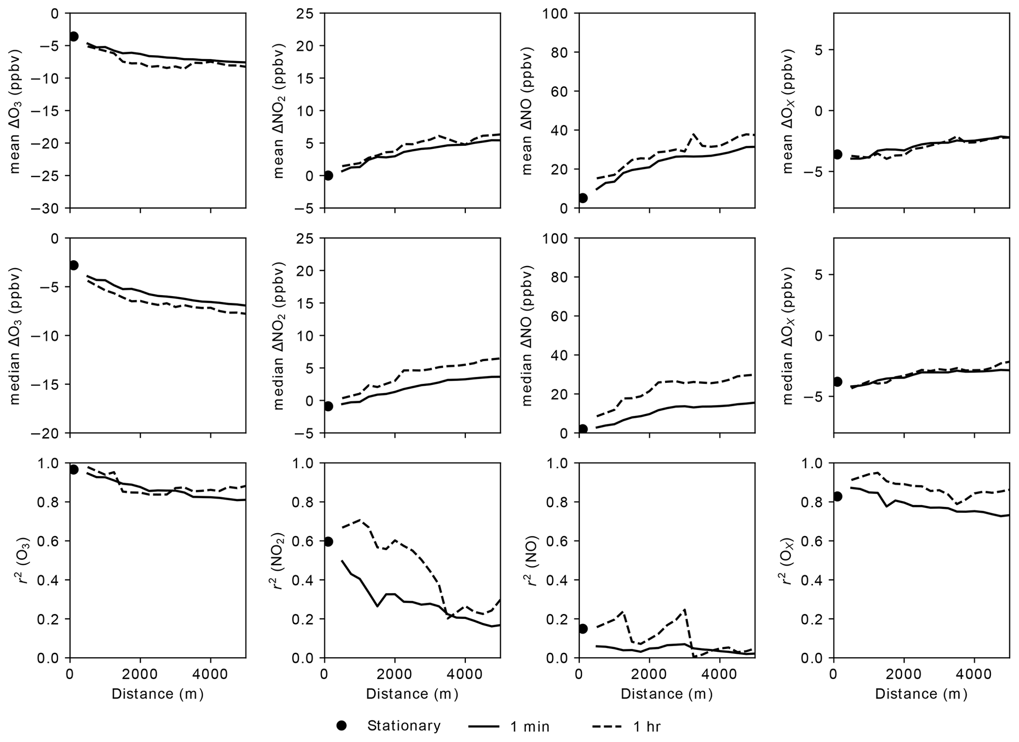
Figure 4Mean and median ΔX and coefficient of determination (r2) for 1 min and 1 h car–La Casa comparisons as a function of the maximum distance between the car and the La Casa site. Results from stationary collocations (Sect. 3) are shown as black dots. All Non-Highway roads are included in this analysis.
5.1 Methods
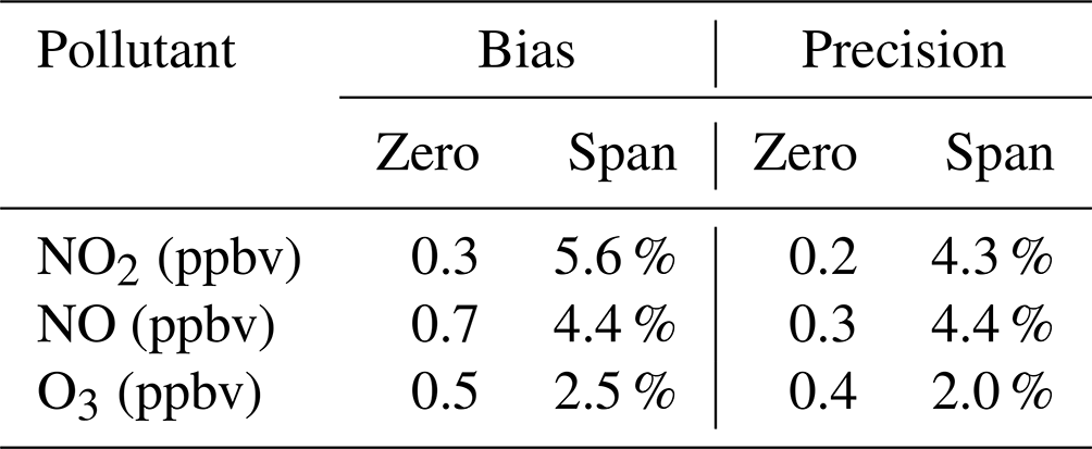
Aclima-operated fleet vehicles are equipped with a mobile sensing device, the Aclima Mobile Node (AMN), which measures carbon monoxide, carbon dioxide, O3, NO, NO2, PM2.5, and total VOCs. The AMN devices are calibrated using the Aclima Mobile Calibration Laboratory (AMCL), a gasoline-powered Ford Transit van equipped with laboratory-grade air pollution measurement instrumentation. The AMCL was driven around the San Francisco Bay Area of California to calibrate the sensors within the AMN devices through comparison of the AMN sensor response with the laboratory-grade equipment collocated in the same van. The laboratory-grade instrumentation in the AMCL is calibrated regularly using reference gases to maintain bias and precision objectives. The calibration procedures have been described in Solomon et al. (2020). Bias and precision results across approximately 25 zero and span checks are shown in Table 2. At the average concentrations observed during the study (11.9 ppbv for NO2, 31.1 ppbv for O3, and 11.9 ppbv for NO), the bias and precision in the span translates to less than 1 ppbv for all three pollutants.
Table 2Precision and bias of measurements in the AMCL from approximately 25 quality assurance (QA) checks during the San Francisco Bay Area study period. Each QA check consisted of a zero and span point for each pollutant.
As part of the validation process, the AMCL regularly drives around several Bay Area Air Quality Management District (BAAQMD) regulatory monitoring sites (Fig. 5). These BAAQMD sites are equipped with EPA-approved FRM and FRM measurements of NO, NO2, and O3 (or a subset of these species), in addition to other pollutants. We present an analysis comparing the AMCL reference measurements with BAAQMD reference measurements between November 2019 and October 2020. All measurements within 10 km of the regulatory sites were included in the dataset used for analysis, as displayed in Fig. 5.
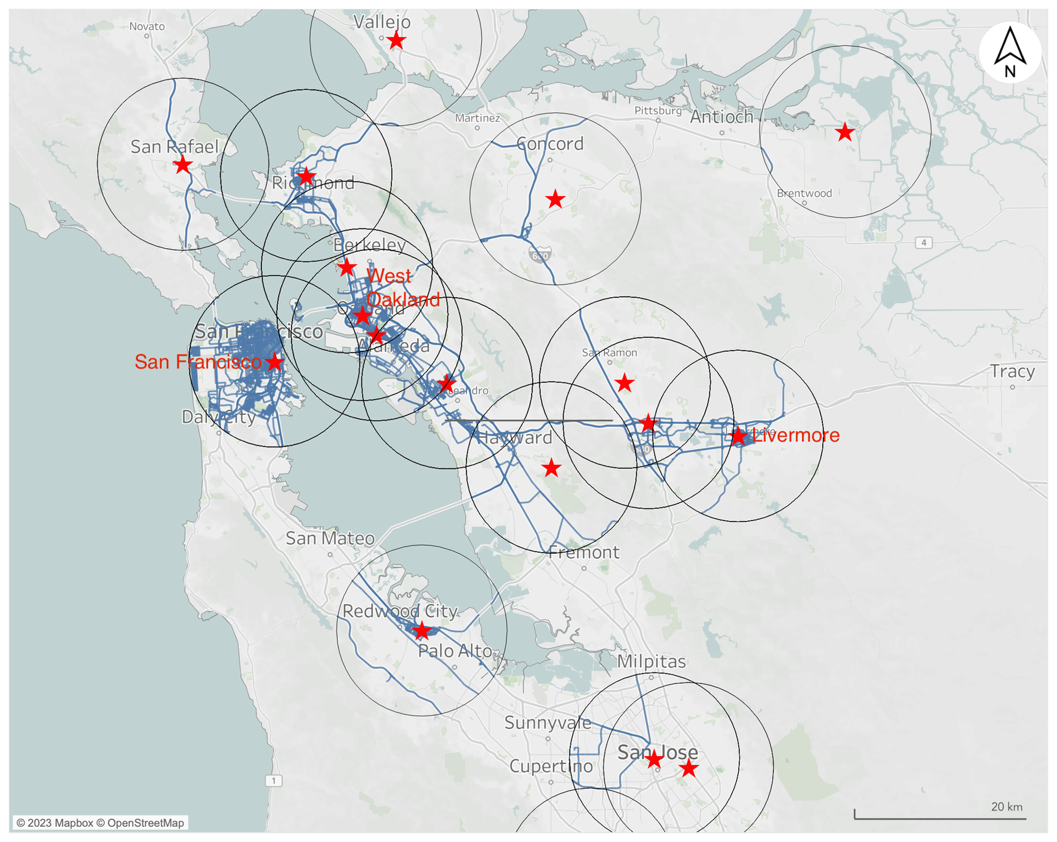
Figure 5Driving patterns around regulatory sites (red stars) in the San Francisco Bay Area. The circles delineate a 10 km radius around each regulatory station. The roads within each circle shown in blue are roads with measurements used in the analysis.
The dataset included comparisons to 19 different BAAQMD sites that represent several spatial representativeness scales (40 CFR 58 Appendix D; Ambient Air Quality Surveillance, 2024). Most of the data were collected near the Livermore, San Francisco, and West Oakland sites. These three regulatory stations are specifically labeled in Fig. 5, and details of the road locations and road types mapped around each site are shown in Fig. 6. Aclima selected these three stations to represent different climatological and land use regimes in the San Francisco Bay Area. The San Francisco station is in a warm-summer Mediterranean climate with marine influence, cool winds, and fog in summer; little overall seasonal temperature variation; and mixed-residential with light industrial land use. The Oakland station has a warm-summer Mediterranean climate with marine influence, overnight fog in the summer, and mixed industrial and residential land use. The Livermore station has a hot-summer Mediterranean climate, inland with some marine influence, and predominantly residential land use; it is also upwind of a large fraction of the urban Bay Area emissions. In contrast to the mapping performed in Denver, measurements near these three monitoring sites generally involved mapping a significant fraction of the roads near the site (Fig. 6). Measurements near other regulatory sites are also included and were generally chance encounters due to the AMCL driving past these sites on its way to its daily mapping assignments, as illustrated in Fig. 5. As a result, these data tend to be from Highways or Major roads and are not mapped as comprehensively on a street-by-street basis.
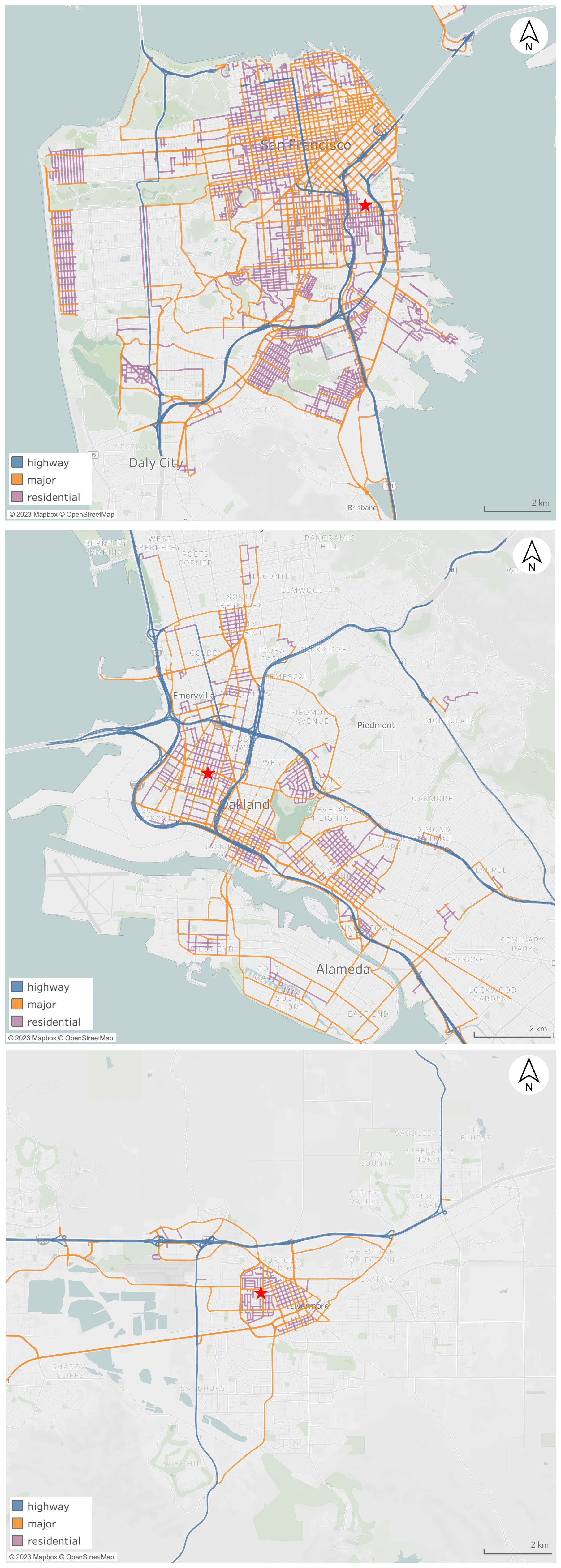
Figure 6Detail of the road locations and road types mapped by the Aclima Mobile Calibration Laboratory around the San Francisco (top), West Oakland (middle), and Livermore (bottom) regulatory sites (indicated by red stars) in the San Francisco Bay Area. Residential roads are shown in purple, Major roads are yellow, and Highway roads are blue.
Based on results from the 2014 Denver dataset (Sect. 4), we focused our analysis on two road-type scenarios – Residential roads and Non-Highway roads. Because the BAAQMD measurements, like most regulatory gas-phase measurements in the USA are reported at a 1 h time resolution, we aggregated each subset of AMCL measurements up to 1 h using the median as an aggregating function. We chose to use the median (versus the mean) to minimize the influence of outliers caused by local traffic emissions. This is in contrast to Sects. 3 and 4, in which the mean was used to aggregate the 1 s data up to 1 min or 1 h. In general, using the median versus the mean produces similar results for O3, NO2, and OX; however, using the hourly medians versus means significantly reduces the impact of high-NO outliers (peaks) on the NO aggregation. The fraction of each 1 h collocation period that included measurements fitting the defined criteria varied depending upon the buffer distance and road-type subset (Figs. S10 and S11 in the Supplement). For smaller distance buffers (e.g., 100 or 300 m) or more restrictive road subsets (e.g., the Residential subset), the distribution was skewed towards a smaller fraction of measurements within each hour fitting the criteria for the comparison. For distance buffers of 1 km or higher on Non-Highway roads, the distribution was approximately uniformly distributed in the 0 %–100 % range. No minimum number of data points was required in each hourly average, such that any individual hourly aggregate may include anywhere between a few seconds and a full hour of 1 Hz mobile-platform data.
5.2 Results and discussion
Using the approach described in Sect. 4.2, both the mean and median bias values and r2 values are shown as a function of road type and distance buffer from the fixed regulatory sites in Fig. 7. Similar to Sect. 4.2, we associated the central tendency of the bias to reflect both instrument biases as well as persistent spatial biases and the r2 values to reflect random spatiotemporal variability. The California study is bolstered by a much larger dataset (note that N in Fig. 7 represents the number of hourly aggregates, whereas the N in Fig. 3 represents the number of 1 min aggregates). This dataset was also collected over a full year and includes comparisons with multiple stationary sites. Despite the different geographic locations and scale of data collection between the California and Denver studies, the general patterns observed in Fig. 7 are highly consistent with the patterns observed in Fig. 3: for example, the higher magnitude of biases and lower r2 at larger buffer distances and significantly worse agreement for Highways than other road classes. The California results do show somewhat higher r2 and a smaller magnitude of biases in general compared with the equivalent hourly averaged results for the Denver study (i.e., the hourly traces in Fig. 4). The higher r2, in particular for NO2, could be due to the larger dataset used, collected over a full year of atmospheric and climatological conditions at multiple sites. This led to both a more representative dataset and a wider range of sampled concentrations than the 1-month, single-site Denver analysis done in Sect. 4. The smaller bias, for O3 and OX, could be due to better inter-lab comparability in the California dataset, but aggregating data across multiple sites may also explain a reduction in the systematic bias. For example, if one site has a slightly positive bias and another site has a slightly negative bias (due to monitor siting or site-to-site calibration variability), those biases will partially cancel each other out. Variances in traffic patterns, road-type distributions, and other factors could also influence differences in biases in different geographic regions or using different driving patterns, so the range of biases must be measured for each individual study region and study design.
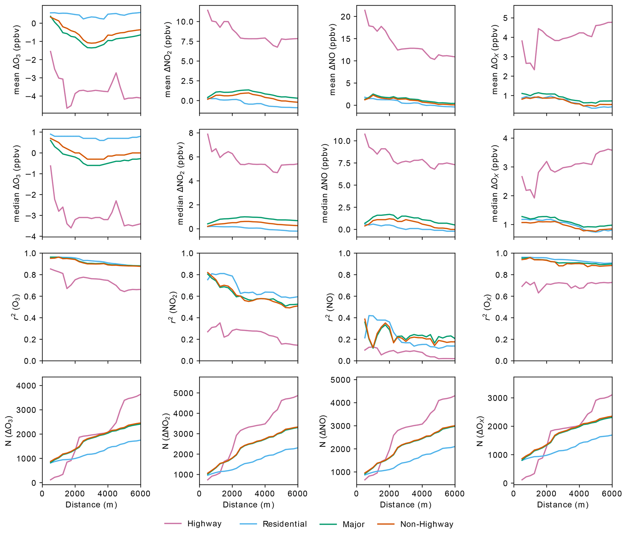
Figure 7Mean and median ΔX, coefficient of determination (r2), and number of data points (N) for 1 h AMCL–regulatory site comparisons as a function of the maximum distance between the AMCL and the regulatory site. Depending upon the buffer distance, the comparisons can include data for up to 19 BAAQMD regulatory sites. Different road classes are shown using different colors.
Figure 7 also shows close agreement between the results for the Major roads and the Non-Highway roads, reflecting the large number of Major roads (versus Residential roads) included in this study compared with Denver. It is interesting to note that the number of data points (N) is almost identical for the Major and Non-Highway road classes. This is because most hour-long periods that included driving on Residential roads also included driving on Major roads, so those hour-long periods were counted separately for the separate Residential and Major road classes but only once for the Non-Highway road classes. Unlike the Denver dataset, this dataset shows remarkable consistency in the r2 values between the Residential, Non-Highway, and Major road classification subsets, suggesting that large-scale application of these comparisons provides similar random spatial biases (r2 values) for Residential and Non-Highway roads. As with the Denver results, there is also minimal variability in these metrics with increasing distance buffers up through 3000 m (and higher).
These results in both Denver and California provide a blueprint for how operational decisions can be made to efficiently collect collocation data to determine systematic measurement bias while accounting for the trade-offs between the rate of data collection and uncertainty tolerance to attribute changes in ΔX to measurement bias. The optimal approach will balance these trade-offs in a way that maximizes N, maximizes r2 (i.e., minimizing random spatial variability), and minimizes the spatial bias component of ΔX. Based on our results in both Denver and California, it is advantageous to remove Highway road segments from the dataset, resulting in a decrease in both the random and the persistent spatiotemporal variability with minimal cost regarding the number of data points collected. Although more complex peak-removal algorithms can achieve similar goals, they add complexity without necessarily improving the comparison and may add additional arbitrary bias (e.g., “cherry-picking”) to the resulting comparisons. A major driving factor for the optimization of the buffer distance and which Non-Highway road types to include is likely to be the rate with which a sufficient number of collocation data points can be collected. For example, consider two end points for this problem: (1) only Residential roads with a buffer distance of 500 m and (2) all Non-Highway roads with a buffer distance of 3000 m. While the Non-Highway roads and large buffer distance would result in a slightly increased bias and random variability over the Residential-road-only and small-buffer-distance scenario, it also is a larger dataset (by a factor of 2–3) and would allow for the simultaneous mapping of a larger area to meet the monitoring objectives more efficiently. Therefore, understanding the impact of the size of the dataset is a critical first step in understanding how to design an operational strategy to use collocations to assess measurement bias.
Quantifying the impact of the size of the dataset requires an analysis along an additional dimension that has not yet been considered: the uncertainty with which ΔX can be determined. While there is likely a close relationship between the magnitude and the uncertainty of ΔX, the uncertainty in ΔX is more important than the absolute value of ΔX in the context of using mobile–stationary comparisons to attribute changes in measurement bias over time. Assuming that random spatial variability is the primary source of error in determining the true systematic spatial bias, the rate at which collocation data can be collected becomes a factor that may need to be weighted more heavily than the absolute magnitude of the spatial bias. This will be especially true for cases where r2 is expected to be low (i.e., for NO2 or NO), which indicates a higher degree of random spatial variability and, therefore, requires additional data collection to achieve an equivalent uncertainty reduction in ΔX. In the following section, we quantify the uncertainty in ΔX as a function of the number of data collected and aggregated.
6.1 Using running median bias values to identify instrument issues
Here, we explore how the number of data aggregated over a specified collection time impacts the instrument bias calculated for the instruments that we know have a stable calibration over time. Our objective is to find the minimum temporal window required to determine reasonable uncertainty bounds for the determination of measurement bias. For the analysis, we use the California dataset of hourly ΔX values and calculate a running median of hourly median ΔX as a function of the number of hours of data in the running average, N. We use median ΔX, as the results are less affected by outliers resulting from local emission plumes and, thus, produce estimates of the bias with smaller magnitude. For this analysis, we focus on a buffer distance of 3000 m and all Non-Highway roads, which results in a sufficiently large dataset to perform this analysis. This scenario is more likely to be encountered in complex urban environments with varied emission sources than a scenario with a narrower buffer distance and solely Residential road types. Figure 8 shows the minimum and maximum bounds for observations of the running median ΔX for the entire dataset as a function of window size N. Note that each individual 1 h ΔX is the median of 1 s differences during that 1 h time window. Therefore, we are taking a running median (over individual hours) of hourly median ΔX values. The range between the upper and lower traces in Fig. 8 provides an estimate of the uncertainty in median ΔX due to random spatial variability, and thus a measure of the magnitude of change in systematic measurement bias that we can expect to be observable by this approach. For each running median window size N, the upper and lower traces reflect the respective maximum and minimum of the set of running N h medians from this dataset. As expected, the range of values decreases with increasing window size, as the influence of random spatial and temporal variability on the calculated bias is reduced. At around a 30–40 h window size, the range between the minimum and maximum stabilizes and does not reduce appreciably with further aggregation.
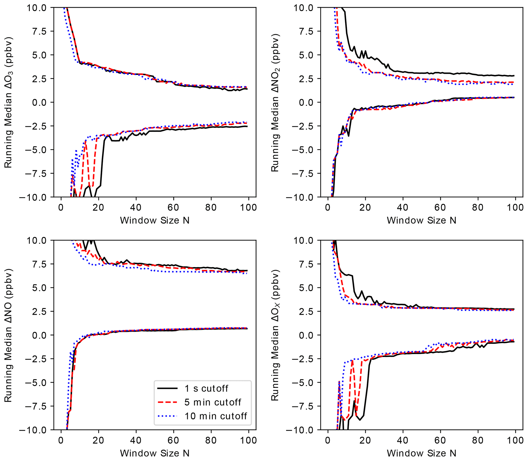
Figure 8Influence of window size on the range (maximum and minimum) of running median ΔO3, ΔNO2, ΔNO, and ΔOX values for all Non-Highway roads within 3 km of a fixed reference site. We show the relationship for three “minimum data” cutoff values – 1 s, 5 min, and 10 min – which define the minimum length of valid data necessary during the hour-long averaging period required to include that hour in the sample dataset.
The number of 1 s data points contributing to each 1 h ΔX value in this analysis is highly variable (Figs. S10, S11). For data within a 3 km buffer distance, the number of 1 s data points in each hour aggregate ranges from just a few seconds to a full hour and is fairly evenly distributed. The time-resolved data from mobile mapping, by nature, can have significant temporal and spatial variability, and using only a few seconds of data to compare to regulatory data with an hourly time resolution may result in additional noise and perhaps invalid assessments of instrument bias in the analysis. To explore the degree to which including hourly aggregates with only a few seconds of data impact the resulting analysis, we repeated the calculation with a restriction on the number of mobile data necessary during each hour-long period for inclusion in the analysis. We used completeness criteria of 5 and 10 min, which would require at least 5 min (or 10 min) of valid data during each hour-long period for that period to be included in the sample dataset for analysis. Note that the 5 or 10 min does not need to have been consecutive. Results are shown alongside the base case (no time-base restriction) in Fig. 8. While there are only subtle differences in the results between the three completeness criteria, the use of a 5 or 10 min minimum cutoff for each hourly aggregation does result in the convergence of median ΔX values at somewhat smaller window sizes, particularly for O3. However, at a rolling window size of around N=40 h or higher, the improvement is marginal (e.g., less than a fraction of a part per billion by volume) in most cases. This analysis has an important implication for the design of a mobile data collection plan that incorporates monitoring in the vicinity of stationary monitors for quality assurance purposes while simultaneously meeting mobile monitoring objectives. The results in Fig. 8 imply that spending only 5–10 min, or even less, within 3 km of a monitoring site can be an effective collocation data point, and the more critical parameter is the number of distinct hourly comparisons. This minimizes the effort needed to collect 40 distinct hours near the monitoring site and, thus, the impact on mobile data collection efficiency in areas of interest farther away from stationary monitors. For the California data used in this analysis, the range of ΔX values of around ± 4 ppbv for O3, NO2, and OX and ± 8 ppbv for NO represent the minimum instrumental drift that we can expect to detect using this method. This is determined as the range between the upper and lower traces in Fig. 8 for each pollutant. We find that it is possible to detect this magnitude of instrumental drift over the time that it takes to collect approximately 40 distinct hourly collocation data points. The time it takes in practices to acquire a 40 h median ΔX depends heavily on the specific data collection plan. For our dataset, we have ∼ 1600 (for O3) to ∼ 1900 (for NO2) hourly data points in our 3 km Non-Highway dataset from 1 year of driving in California. For a rolling window size of 40, this gives an “effective response time” on the order of 1 week (7–9 d), where the response time is the study period (365 d) divided by the number of discrete hour-long periods (1600–1900) multiplied by the rolling window size (40). This response time is likely atypical, as the objective of this monitoring plan was specifically to collect data in close proximity to a predetermined set of stationary monitors. On the other hand, most typical mobile monitoring deployments would aim to collect over a much broader area, and there would be much higher value in collecting in areas farther removed from where stationary monitors exist. Nevertheless, it does provide a framework for planning purposes. For example, if it is desirable to detect instrumental drift over a quarterly time period, the mobile collection plan would need to incorporate about three separate visits per week to Non-Highway roads within a 3 km radius of a stationary monitor. Importantly, these visits do not need to be exclusively 1 h long visits, and visits of only 5–10 min or even a few seconds can be viable. While imposing a minimum data completeness criteria might improve the range of running median ΔX values at lower N values, it comes at the cost of a reduction in the number of data and, thus, an increase in the effective response time (for similar values of N).
Using a running 40 h time window, we show a time series of hourly median ΔO3, ΔNO2, ΔNO, and ΔOX in Fig. 9. Both the raw 1 h data (red points) and the 40 h running median (black line) are included. While there is a large degree of variability for any individual ΔX value, the running median reduces that random variability and provides an estimate with quantified uncertainty bounds that can be used to identify drift. For long-term driving campaigns that frequently pass near stationary monitoring sites, this method appears to be a practical way to monitor systematic bias in mobile measurements in an ongoing basis. In Sect. 6.2, we apply this method to an example of two NO2 sensors in Aclima's mobile fleet to show how this method could identify real drift in lower-cost sensors.
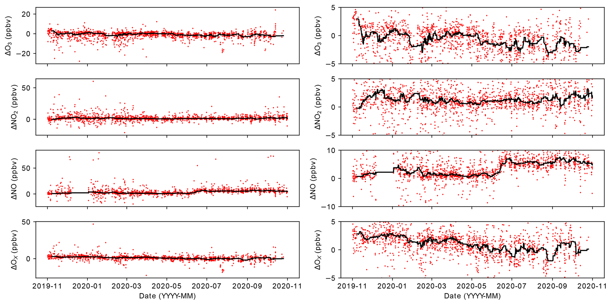
Figure 9Time series of 3 km ΔO3, ΔNO2, ΔNO, and ΔOX, showing individual 1 h measurements (red points) and 40 h running medians (solid line). The right column truncates many of the 1 h measurements and scales the y axis to highlight the range of the running median values.
6.2 Case study: NO2 sensors in Aclima's mobile fleet
To illustrate how the running median method can be used to identify drift in sensors deployed for mobile monitoring, we show an example using NO2 sensors deployed as part of Aclima's mobile collection fleet. We analyzed mobile–stationary differences for two NO2 sensors deployed in two different vehicles across a multi-month deployment in California. In contrast to the AMCL results shown in Sects. 5 and 6.1, these sensors are not regularly calibrated during their mobile deployments. Instead, they are calibrated initially via collocation with the reference instruments in the AMCL (prior to deployment) and calibrated a second time in the AMCL at the end of their deployment period. For Sensor A, the original calibration was found to have held well during the post-deployment calibration check, with a mean bias of +2.2 ppbv. This was well within our ± 6 ppbv acceptance criteria for the NO2 sensor. Sensor B, in contrast, was found to have a mean bias of −15.5 ppbv during its post-deployment calibration check, indicating significant drift beyond what we consider acceptable performance.
While the sensors are deployed, the only possible in situ evaluation of the calibration of these sensors was using mobile–stationary comparisons with fixed reference sites. Over the course of the deployment for both vehicles, they made frequent passes within 3000 m of various regulatory sites. These sites were not specifically targeted; rather, these encounters occurred over the course of typical data collection for hyperlocal air pollution mapping. The hour-averaged results for each of these sensors are shown in Fig. 10 along with the 40 h running median. The in situ running median biases compared to the regulatory sites are consistent with the post-deployment bias determinations, indicating that mobile–stationary comparisons could be used to detect drift in mobile NO2 sensors during deployment. In addition, it is apparent in Fig. 10 that Sensor B had significant discrepancies compared with the fixed reference sites that were outside of the expected ± 6 ppbv uncertainties. Therefore, this method could have been used to identify potential issues with Sensor B during deployment without waiting until a post-deployment calibration. While a more detailed analysis across multiple devices and deployments would be required to establish this approach as an accepted method, this case study demonstrates how such an approach might be feasible.
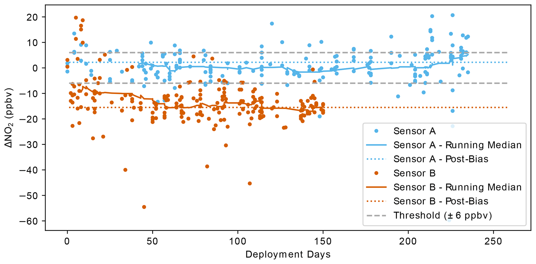
Figure 10Time series of 1 h ΔNO2 and 40 h running medians for two sensors (Sensor A and Sensor B) deployed as part of Aclima NO2 sensor deployment. Uncertainty threshold (± 6 ppbv) and post-campaign sensor biases are also shown.
In this paper, we focus on three major pollutants (O3, NO2, and NO) with very different behaviors in the atmosphere. O3 is predominantly a regionally distributed secondary pollutant with high background concentrations and negative deviations in direct emission plumes, especially those containing NO (which rapidly titrates O3). NO2 is both a primary and secondary pollutant that has moderate regional background concentrations and falls into the category of a co-emitted pollutant with high regional background (Brantley et al., 2014), along with species like fine particulate matter (PM2.5) and coarse particulate matter (PM10). NO is a primary pollutant with a short lifetime, especially in the presence of O3, and has high peak concentrations and low background concentrations. NO falls into the category of a co-emitted pollutant with a low regional background (Brantley et al., 2014), which also includes pollutants such as carbon monoxide, black carbon, and ultrafine particles.
In addition to providing valuable insights into deployed sensor data quality, our analysis also provides information about the spatial heterogeneity of these atmospheric pollutants and the spatial representativeness of measurements at stationary sites. If we consider the coefficient of determination (r2) of the mobile–stationary regressions to be a simple proxy for spatial homogeneity (setting aside the important temporal component to this variability for now), with higher r2 indicating a more spatially homogeneous pollutant, then we conclude that O3 is more spatially homogeneous, NO is more heterogeneous, and NO2 is between the two. This is consistent with our understanding of emission sources and atmospheric lifetimes of these different species under typical urban conditions. The temporal component of this spatial variability is, of course, a key consideration and, as such, the linear regressions described by the r2 values (and shown in Fig. S12 in the Supplement) are sensitive to the spatial variability within an hourly snapshot, while the relationships shown in Fig. 8 describe the spatial variability over different temporal aggregations (i.e., the median window size). The field of hyperlocal air quality monitoring is predicated on the fundamental principle that aggregating many samples over time is required to reduce the impact of temporal variability to observe persistent spatial trends in concentration (Apte et al., 2017; Messier et al., 2018; Van Poppel et al., 2013). While the hourly variability between mobile and stationary measurements may be a reasonable proxy for spatial heterogeneity, aggregations over longer durations provide a more accurate measure.
The high degree of correlation between hourly mobile and stationary measurements might suggest that O3 has minimal spatial variability. However, our analysis shows that there are measurable spatial gradients in O3. This is particularly true for Highways and, to a lesser degree, Major roads, compared with Residential roads and stationary sites. Figure 3, for example, clearly shows observable differences in the mobile measurements in Denver compared with the stationary measurements, both as a function of distance from the site and as a function of road type. For this reason, our analysis intentionally removes highways specifically to reduce the influence of local emission plumes in the dataset so that the mobile to stationary comparison can be more readily indicative of measurement bias. However, the full dataset could offer a means to more closely investigate the interplay between the hyperlocal spatial patterns of these three closely related pollutants (O3, NO2, and NO) and the implications for effective emissions controls at hyperlocal scales.
This relationship between spatial heterogeneity, mobile–stationary correlation coefficients, and the practicality of using mobile–stationary comparisons as a quality control method suggests that it is possible to make some educated assumptions about how other pollutants would behave. For example, PM2.5 has both primary and secondary sources and would likely show mobile to stationary correlations similar to NO2, or possibly O3 in some areas. Conversely, black carbon, carbon monoxide, or ultrafine particles would likely behave more similarly to NO, given their variability in near-source-area results primarily from direct emissions. While we expect significant differences in correlation with stationary sites for different pollutants across the spectrum of spatial variability, the results in Fig. 8 for NO, NO2, and O3 suggest that all pollutants would likely follow a similar pattern of decreasing range of ΔX with increasing median window size. The key differences that would be expected for different pollutants would be the optimal median window size (although the optimal median window size is similar for all three measured pollutants in this study) and the width of the confidence intervals around the central tendency of the differences between mobile and stationary measurements and, thus, the magnitude of systematic measurement bias that could be detected.
In this paper, we address the issue of ongoing quality assurance during a large-scale mobile monitoring campaign, with a focus on discerning changes in instrument performance over time during mobile-platform deployment. To assess instrumental drift over time using any sort of collocation or sensor–reference comparison, it is first necessary to constrain the uncertainty inherent in the collocation or comparison process. We used a set of parked and moving mobile monitoring data from a 1-month study in Denver, CO, in 2014 and compared reference-grade NO, NO2, and O3 measurements from a mobile platform to fixed-reference-site measurements both when the mobile platform was parked side-by-side with the reference site and when driving at distances out to several kilometers from the reference site. Using data from a more extensive, 1-year study in California (starting November 2019), we show large-scale comparisons of hourly mean mobile measurements to hourly fixed-reference-site measurements. We highlight the importance of grouping data based on street type to reduce the influence of emission plumes, which are most abundant on highways. We demonstrate a possible data aggregation technique for large-scale, long-term comparisons. Hourly averaged regulatory site data are reported by most state and local air quality monitoring agencies in the USA and many other countries. These hourly aggregated mobile-platform measurements show excellent agreement with hourly averaged fixed-site measurements using running medians of moving mobile–fixed-site differences. The work presented here will be extended in the future to examine how these methodologies can be used to assess the ongoing performance of low-cost sensor nodes in mobile monitoring platforms.
The data used in this paper are proprietary and are owned by Aclima, Inc. Interested researchers are encouraged to contact Aclima, Inc. for data availability and collaboration opportunities. Additional questions about analysis techniques or code can be directed to the corresponding author of this paper.
The supplement related to this article is available online at: https://doi.org/10.5194/amt-17-2991-2024-supplement.
ML, SK, and PS: conceptualization; ML and BL: data curation; AW, ML, and BL: formal analysis; ML, BL, and PS: funding acquisition; AW, ML, and BL: investigation; AW, ML, BL, and PS: methodology; ML, SK, and PS: project administration; ML, BL, and PS: resources; AW, ML, and BL: software; ML, SK, and PS: supervision; ML, BL, and PS: validation; AW and ML: visualization; AW, ML, and BL: writing – original draft; AW, ML, BL, and PS: writing – review and editing.
The contact author has declared that none of the authors has any competing interests.
This paper was subjected to internal review at the United States Environmental Protection Agency (US EPA) and has been cleared for publication. Mention of trade names or commercial products does not constitute endorsement or recommendation for use. The views expressed in this article are those of the author(s) and do not necessarily represent the views or policies of the US EPA.
Publisher's note: Copernicus Publications remains neutral with regard to jurisdictional claims made in the text, published maps, institutional affiliations, or any other geographical representation in this paper. While Copernicus Publications makes every effort to include appropriate place names, the final responsibility lies with the authors.
The project was conducted in part under a cooperative research and development agreement between the US EPA and Aclima, Inc. (EPA CRADA no. 734-13, 13 April 2013, and Amendment 734-A14, to 13 April 2023). The authors would like to thank the internal technical and management reviewers from the US EPA, including Shaibal Mukerjee, Robert Vanderpool, Libby Nessley, Michael Hays, and Lara Phelps, for their excellent suggestions regarding modifications and improvements to the draft manuscript. The authors would like to thank US EPA Region 8 for support of the project in Denver and the data sharing cooperation from DISCOVER-AQ and the Colorado Department of Public Health and Environment. We gratefully acknowledge Davida Herzl and Karin Tuxen-Bettman, for their vision and support, and Christian Kremer, Matthew Chow, Cassie Trickett, Marek Kwasnica, and the Aclima Technical Operations Team, for the dedicated support of Aclima's data quality operations.
This paper was edited by Albert Presto and reviewed by three anonymous referees.
Alas, H. D. C., Weinhold, K., Costabile, F., Di Ianni, A., Müller, T., Pfeifer, S., Di Liberto, L., Turner, J. R., and Wiedensohler, A.: Methodology for high-quality mobile measurement with focus on black carbon and particle mass concentrations, Atmos. Meas. Tech., 12, 4697–4712, https://doi.org/10.5194/amt-12-4697-2019, 2019.
Ambient Air Quality Surveillance, 40 C.F.R. pt. 58, https://www.ecfr.gov/current/title-40/chapter-I/subchapter-C/part-58 (last access: 9 May 2024), 2024.
Apte, J. S., Messier, K. P., Gani, S., Brauer, M., Kirchstetter, T. W., Lunden, M. M., Marshall, J. D., Portier, C. J., Vermeulen, R. C. H., and Hamburg, S. P.: High-Resolution Air Pollution Mapping with Google Street View Cars: Exploiting Big Data, Environ. Sci. Technol., 51, 6999–7008, https://doi.org/10.1021/acs.est.7b00891, 2017.
Bauerová, P., Šindelářová, A., Rychlík, Š., Novák, Z., and Keder, J.: Low-Cost Air Quality Sensors: One-Year Field Comparative Measurement of Different Gas Sensors and Particle Counters with Reference Monitors at Tušimice Observatory, Atmosphere, 11, 492, https://doi.org/10.3390/atmos11050492, 2020.
Brantley, H. L., Hagler, G. S. W., Kimbrough, E. S., Williams, R. W., Mukerjee, S., and Neas, L. M.: Mobile air monitoring data-processing strategies and effects on spatial air pollution trends, Atmos. Meas. Tech., 7, 2169–2183, https://doi.org/10.5194/amt-7-2169-2014, 2014.
Castell, N., Dauge, F. R., Schneider, P., Vogt, M., Lerner, U., Fishbain, B., Broday, D., and Bartonova, A.: Can commercial low-cost sensor platforms contribute to air quality monitoring and exposure estimates?, Environ. Int., 99, 293–302, https://doi.org/10.1016/j.envint.2016.12.007, 2017.
Chambliss, S. E., Pinon, C. P. R., Messier, K. P., LaFranchi, B., Upperman, C. R., Lunden, M. M., Robinson, A. L., Marshall, J. D., and Apte, J. S.: Local- and regional-scale racial and ethnic disparities in air pollution determined by long-term mobile monitoring, P. Natl. Acad. Sci. USA, 118, e2109249118, https://doi.org/10.1073/pnas.2109249118, 2021.
Clements, A. L., Griswold, W. G., Abhijid, R. S., Johnston, J. E., Herting, M. M., Thorson, J., Collier-Oxandale, A., and Hannigan, M.: Low-Cost Air Quality Monitoring Tools: From Research to Practice (A Workshop Summary), Sensors, 17, 2478, https://doi.org/10.3390/s17112478, 2017.
Collier-Oxandale, A., Feenstra, B., Papapostolou, V., Zhang, H., Kuang, M., Der Boghossian, B., and Polidori, A.: Field and laboratory performance evaluations of 28 gas-phase air quality sensors by the AQ-SPEC program, Atmos. Environ., 220, 117092, https://doi.org/10.1016/j.atmosenv.2019.117092, 2020.
Kebabian, P. L., Herndon, S. C., and Freedman, A.: Detection of Nitrogen Dioxide by Cavity Attenuated Phase Shift Spectroscopy, Anal. Chem., 77, 724–728, https://doi.org/10.1021/ac048715y, 2005.
Li, Y., Yuan, Z., Chen, L. W. A., Pillarisetti, A., Yadav, V., Wu, M., Cui, H., and Zhao, C.: From air quality sensors to sensor networks: Things we need to learn, Sensor. Actuat. B-Chem., 351, 130958, https://doi.org/10.1016/j.snb.2021.130958, 2022.
Long, R. W., Whitehill, A., Habel, A., Urbanski, S., Halliday, H., Colón, M., Kaushik, S., and Landis, M. S.: Comparison of ozone measurement methods in biomass burning smoke: an evaluation under field and laboratory conditions, Atmos. Meas. Tech., 14, 1783–1800, https://doi.org/10.5194/amt-14-1783-2021, 2021.
Masey, N., Gillespie, J., Ezani, E., Lin, C., Wu, H., Ferguson, N. S., Hamilton, S., Heal, M. R., and Beverland, I. J.: Temporal changes in field calibration relationships for Aeroqual S500 O3 and NO2 sensor-based monitors, Sensor. Actuat. B-Chem., 273, 1800–1806, https://doi.org/10.1016/j.snb.2018.07.087, 2018.
Messier, K. P., Chambliss, S. E., Gani, S., Alvarez, R., Brauer, M., Choi, J. J., Hamburg, S. P., Kerckhoffs, J., LaFranchi, B., Lunden, M. M., Marshall, J. D., Portier, C. J., Roy, A., Szpiro, A. A., Vermeulen, R. C. H., and Apte, J. S.: Mapping Air Pollution with Google Street View Cars: Efficient Approaches with Mobile Monitoring and Land Use Regression, Environ. Sci. Technol., 52, 12563–12572, https://doi.org/10.1021/acs.est.8b03395, 2018.
Solomon, P. A., Vallano, D., Lunden, M., LaFranchi, B., Blanchard, C. L., and Shaw, S. L.: Mobile-platform measurement of air pollutant concentrations in California: performance assessment, statistical methods for evaluating spatial variations, and spatial representativeness, Atmos. Meas. Tech., 13, 3277–3301, https://doi.org/10.5194/amt-13-3277-2020, 2020.
Environmental Protection Agency: Office of Research and Development; Ambient Air Monitoring Reference and Equivalent Methods: Designation of Four New Equivalent Methods, 79 FR 34734, https://www.federalregister.gov/documents/2014/06/18/2014-14249/office-of-research-and-development-ambient-air-monitoring-reference-and-equivalent-methods, last access: 18 June 2014.
Van Poppel, M., Peters, J., and Bleux, N.: Methodology for setup and data processing of mobile air quality measurements to assess the spatial variability of concentrations in urban environments, Environ. Pollut., 183, 224–233, https://doi.org/10.1016/j.envpol.2013.02.020, 2013.
Wang, S., Ma, Y., Wang, Z., Wang, L., Chi, X., Ding, A., Yao, M., Li, Y., Li, Q., Wu, M., Zhang, L., Xiao, Y., and Zhang, Y.: Mobile monitoring of urban air quality at high spatial resolution by low-cost sensors: impacts of COVID-19 pandemic lockdown, Atmos. Chem. Phys., 21, 7199–7215, https://doi.org/10.5194/acp-21-7199-2021, 2021.
Weissert, L., Alberti, K., Miles, E., Miskell, G., Feenstra, B., Henshaw, G. S., Papapostolou, V., Patel, H., Polidori, A., Salmond, J. A., and Williams, D. E.: Low-cost sensor networks and land-use regression: Interpolating nitrogen dioxide concentration at high temporal and spatial resolution in Southern California, Atmos. Environ., 223, 117287, https://doi.org/10.1016/j.atmosenv.2020.117287, 2020.
Whitehill, A. R., Lunden, M., Kaushik, S., and Solomon, P.: Uncertainty in collocated mobile measurements of air quality, Atmospheric Environment: X, 7, 100080, https://doi.org/10.1016/j.aeaoa.2020.100080, 2020.
- Abstract
- Introduction
- Instrumentation used in this study
- Mobile platforms parked at fixed reference sites in Denver (2014)
- Mobile platforms driving around a fixed reference site in Denver (2014)
- Mobile platforms driving around fixed reference sites in California (2019–2020)
- Operationalization of mobile–fixed site comparisons for ongoing instrument assessment
- Spatial heterogeneity and implications for applicability to additional pollutants
- Conclusions
- Data availability
- Author contributions
- Competing interests
- Disclaimer
- Acknowledgements
- Review statement
- References
- Supplement