Multiple-scattering effects on single-wavelength lidar sounding of multi-layered clouds

We performed Monte Carlo simulations of single-wavelength lidar signals from multi-layered clouds with special attention focused on the multiple-scattering (MS) effect in regions of the cloud-free molecular atmosphere (i.e. between layers or outside a cloud system). Despite the fact that the strength of lidar signals from the molecular atmosphere is much lower compared to the in-cloud intervals, studies of MS effects in such regions are of interest from scientific and practical points of view.

The MS effect on lidar signals always decreases with the increasing distance from the cloud far edge. The decrease is the direct consequence of the fact that the forward peak of particle phase functions is much larger than the receiver field of view (RFOV). Therefore, the photons scattered within the forward peak escape the sampling volume formed by the RFOV (i.e. the escape effect). We demonstrated that the escape effect is an inherent part of MS properties within the free atmosphere beyond the cloud far edge.

In the cases of the ground-based lidar, the MS contribution is lower than 5 % within the regions of the cloud-free molecular atmosphere with a distance from the cloud far edge of about 1 km or higher. In the cases of the space-borne lidar, the rate of decrease of the MS contribution is so slow that the threshold of 5 % can hardly be reached. In addition, the effect of non-uniform beam filling is extremely strong. Therefore, practitioners should employ, with proper precautions, lidar data from regions below the cloud base when treating data of a space-borne lidar.

In the case of two-layered cloud, the distance of 1 km is sufficiently large so that the scattered photons emerging from the first layer do not affect signals from the second layer when we are dealing with the ground-based lidar. In contrast, signals from the near edge of the second cloud layer are severely affected by the photons emerging from the first layer in the case of a space-borne lidar.

We evaluated the Eloranta model (EM) in extreme conditions and showed its good performance in the cases of ground-based and space-borne lidars. At the same time, we revealed the shortcoming that can affect practical applications of the EM. Namely, values of the key parameters – i.e. the ratios of phase functions in the backscatter direction for the nth-order-scattered photon and a singly scattered photon – depend not only on the particle phase function but also on the distance from a lidar to the cloud and the receiver field of view. Those ratios vary within a quite large range, and the MS contribution to lidar signals can be largely overestimated or underestimated if erroneous values of the ratios are assigned to the EM.

1 Introduction

It is well recognized that multiple scattering (MS) inevitably affects the data of space-borne lidars (see e.g. Winker, 2003; Young and Vaughan, 2009; Shcherbakov et al., 2022). As for ground-based lidars, the MS relative contribution to lidar signals can exceed 20 % even in the case of cirrus clouds with an extinction coefficient of ε_p=0.2 km⁻¹ and can reach 200 % when ε_p=1.0 km⁻¹ (Shcherbakov et al., 2022). On the other hand, the MS effect is within measurement errors of ground-based and airborne lidars – i.e. the single-scattering (SS) approximation – can be used when the receiver field of view (RFOV) is quite narrow and/or the extinction coefficient is quite low (Shcherbakov et al., 2022).

Lidar signals are used as input data to retrieve profiles of the characteristics of interest – e.g. the extinction coefficient, the backscatter coefficient, and the lidar ratio (see e.g. Young and Vaughan, 2009). If the MS contribution cannot be neglected, a solution to the corresponding inverse problem has to take into account the MS effect in order to avoid biased retrievals. To put it differently, a correction for the effects of multiple scattering has to be applied (Young and Vaughan, 2009).

Generally, any algorithm to solve an inverse problem is based on a solution to the corresponding direct, i.e. forward problem (see e.g. Rodgers, 2000; Neto and Neto, 2013). It is obvious that retrieval quality is closely related to the accuracy of the direct modelling. To put it in relation to lidar sounding, the quality of the correction for MS effects directly depends on the accuracy of lidar signal modelling in multiple-scattering conditions.

Expressed mathematically, any modelling in MS conditions has to be based on the radiative transfer equation and corresponding boundary conditions (see e.g. Marchuk et al., 2013). It is well known that there exist only a few cases when a solution to the radiative transfer equation can be obtained as an analytical expression. Thus, numerical methods – e.g. Monte Carlo (MC) simulations (Marchuk et al., 2013) or approximate models – are largely applied to obtain solutions. Referring to lidar sounding, a good review of developed approximate methods and models can be found in Bissonnette (2005). Using some cases as examples, good performance of approximate models was underlined by their authors. At the same time, we believe that the accuracy level and the applicability bounds of approximate models still need to be rigorously evaluated.

What was suggested in the work by Weinman (1968) was approximating a phase function of cloud particles by a somewhat smoothly varying function of the scattering angle plus a narrow Gaussian peak for small angles. That idea was used to develop models that simulate lidar signals in multiple-scattering conditions, and promising results were obtained (see e.g. Eloranta, 1998; Hogan, 2006, 2008). For example, good agreement with MC simulations of the second, third, and fourth order of scattering was shown for the case of an extinction coefficient of 16.7 km⁻¹ (Eloranta, 1998). Moreover, the models (Eloranta, 1998; Hogan, 2006, 2008) were employed by practitioners to account for MS effects while retrieving clouds' optical properties on the basis of experimental lidar data (see e.g. Nakoudi et al., 2021; Seifert et al., 2007; Delanoë and Hogan, 2008).

On the other hand, results of MC simulations published in the literature (see e.g. Flesia and Starkov, 1996; Donovan, 2016; Reverdy et al., 2015; Szczap et al., 2021) evidenced the following. As it is expected, lidar signals from regions of the cloud-free molecular atmosphere – namely between cloud layers and/or beyond the far edge of a cloud system – are affected by the scattered light emerging from clouds. To our knowledge, optical processes and cloud characteristics that govern the effect on lidar signals of the emerging light (i.e. the MS effect) and its distinctive features have not been addressed in detail in the literature.

The main objective of this work is to perform Monte Carlo simulations of single-wavelength lidar signals from multi-layered clouds with special attention focused on the peculiarities of the MS effect in regions of the cloud-free molecular atmosphere – i.e. between layers or outside a cloud system. In our opinion, such a study helps to obtain further insight into the problem that is MS effects. At the same time, it has practical applications because some inverse-problem algorithms use lidar data taken from the range of the cloud-free atmosphere beyond the far edge of a cloud – for example, the two-way transmittance method (see e.g. Young and Vaughan, 2009; Giannakaki et al., 2007; and references therein).

The second objective of this work is to evaluate the performance of an approximate model with the focus on the cloud-free regions. We have chosen for the evaluation the model developed by Eloranta (1998) because multiple integrals are in its core (see Eq. 11 in Eloranta, 1998, and Eqs. 3–4 in Eloranta, 2000). A code to compute multiple integrals belongs to the domain of basic programming tasks. Therefore, it is an easy matter to develop a code corresponding to the Eloranta model.

Throughout this work, the majority of the results are shown and discussed in terms of relative contributions of multiple scattering (see definitions in Sect. 2.1) – that is, multiple-to-single-scattering lidar return ratios (Bissonnette et al., 1995). At the same time, the reader should keep in mind that the ratios do not show lidar signals but the relative contribution of MS with respect to lidar signals obtained under the SS approximation. From the point of view of the inverse problem, the ratios are of key importance because they show the level of retrieval errors if the SS approximation were applied in an inversion algorithm. If different models, which simulate the direct problem, are compared, the ratios clearly evidence the differences between the results (see e.g. Bissonnette et al., 1995). In our opinion, a comparison between lidar signals instead of between ratios suffers from a severe disadvantage for the following reasons. Even when lidar signals are corrected for the offset and instrumental factors, they do decrease exponentially because of the extinction. Consequently, the semi-logarithmic plot is usually employed to show data, and even important differences are hardly noticeable in such figures. Moreover, when differences are seen, it is difficult for the reader to estimate their importance from the point of view of the inverse problem.

The MS effect on lidar signals depends on a number of parameters – namely, the configuration (the distance to a cloud; the emitter field of view, EFOV; and the RFOV) and the cloud optical characteristics (the extinction coefficient, the albedo, the scattering matrix, and so on) (see e.g. Shcherbakov et al., 2022, and references therein). Because the MC method is very time-consuming, it is not suited for taking into account variations in all parameters mentioned. Therefore, our study was restricted to the cases when all cloud layers were within the range between the altitudes of 8 and 11 km. Almost all MC simulations were performed for cloud particles with an extinction coefficient of ε_p(h)=1.0 km⁻¹ for the following reasons. On the one hand, technical capacities of contemporary lidars provide us with the possibility of recording signals from the cloud-free atmosphere beyond the far edge of a cloud with an optical thickness of τ_p=3.0. On the other hand, the MS effect cannot be neglected and is clearly seen in a number of cases (Shcherbakov et al., 2022). Our choice of the parameter values was deliberate despite the fact that the altitude range H∈[8, 11 ] km does not correspond to the usual altitudes of warm clouds and that the value ε_p(h)=1.0 km⁻¹ is quite small for water clouds and rather high for cirrus clouds. With such a choice, the phase-function impact on multiple scattering is free of the interference of other parameter variations.

For the sake of brevity, the term “sampling volume” is used in this work in reference to the volume bounded by the RFOV of a lidar in 3D space.

Section 2 addresses the methodology of our Monte Carlo simulations in detail. Sections 3 and 4 show our simulation results for a ground-based and a space-borne lidar, respectively. Section 5 is devoted to conclusions. Appendix A is focused on the Eloranta model and its input parameters in homogeneous-cloud conditions; Appendix B is devoted to the simulation uncertainty analysis.

2 Methodology

2.1 Background

We use the following notations in this work. The function S₁(h) characterizes lidar signals under the SS approximation (corrected for the offset, the instrumental factors, and the two-way ozone transmittance):

$$\begin{array}{}\text{(1)}& \begin{array}{rl}{S}_{\mathrm{1}}\left(h\right)& =\left[{\mathit{\beta }}_{\mathrm{p}}\left(h\right)+{\mathit{\beta }}_{\mathrm{m}}\left(h\right)\right]\cdot T^{\mathrm{2}}\left(h\right)=\left[{\mathit{\beta }}_{\mathrm{p}}\left(h\right)+{\mathit{\beta }}_{\mathrm{m}}\left(h\right)\right]\\ & \cdot T_{\mathrm{m}}^{\mathrm{2}}\left(h\right)\cdot T_{\mathrm{p}}^{\mathrm{2}}\left(h\right),\end{array}\end{array}$$

where h is the distance from the lidar; β_p(h) and β_m(h) represent the backscatter contributions from particles and from the atmospheric molecules; $T^{\mathrm{2}}\left(h\right)=T_{\mathrm{m}}^{\mathrm{2}}\left(h\right)\cdot T_{\mathrm{p}}^{\mathrm{2}}\left(h\right)$ is the two-way transmittance from the lidar to the range, h; and $T_{\mathrm{m}}^{\mathrm{2}}\left(h\right)$ and $T_{\mathrm{p}}^{\mathrm{2}}\left(h\right)$ are the molecular and the particulate transmittances, respectively. $T_{\mathrm{p}}^{\mathrm{2}}\left(h\right)=\mathrm{1}$ if h≤h_b, where h_b is the distance to the cloud near edge; $T_{\mathrm{p}}^{\mathrm{2}}\left(h\right)=\exp \left[-\mathrm{2}{\mathit{\tau }}_{\mathrm{p}}\left(h_{\mathrm{b}},h\right)\right]$ when h≥h_b, where ${\mathit{\tau }}_{\mathrm{p}}\left(h_{\mathrm{b}},h\right)={\int }_{h_{\mathrm{b}}}^h{\mathit{\epsilon }}_{\mathrm{p}}\left(h^{\prime }\right)\mathrm{d}{h}^{\prime }$ is the cloud optical depth and ε_p(h) is the extinction coefficient of particles.

The notation S_k(h), k=2, 3, …, n, represents lidar signals (corrected for the offset, the instrumental factors, and the two-way ozone transmittance) when all scattering events from the first (single scattering) up to the kth inclusive are taken into account; (k+1)th and higher orders of scattering are neglected. For example, S₂(h) is the double-scattering (DS) approximation (see e.g. Bissonnette, 2005). The notation S_MS(h) means that all scattering events are taken into consideration. Of course, only S_MS(h) can be obtained from real lidar measurements. S_k(h) carries useful data of simulations computed with the Monte Carlo method or an approximate model.

Below, we use the following characteristics to compare the simulations results:

$$\begin{array}{}\text{(2)}& {\displaystyle }{R}_{\mathrm{k}to\mathrm{1}}\left(h\right)=\left[S_k\left(h\right)-S_{k-\mathrm{1}}\left(h\right)\right]/S_{\mathrm{1}}\left(h\right),\text{(3)}& {\displaystyle }{R}_{\mathrm{MSto}\mathrm{1}}\left(h\right)=\left[S_{\mathrm{MS}}\left(h\right)-S_{\mathrm{1}}\left(h\right)\right]/S_{\mathrm{1}}\left(h\right).\end{array}$$

The ratio R_kto1(h) is the relative contribution of the kth order of scattering to a lidar signal. For example, $R_{\mathrm{4}\mathrm{to}\mathrm{1}}\left(h\right)=\left[S_{\mathrm{4}}\left(h\right)-S_{\mathrm{3}}\left(h\right)\right]/S_{\mathrm{1}}\left(h\right)$ provides the relative contribution of the fourth order of scattering. The ratio R_MSto1(h) is the relative contribution of multiple scattering to a lidar signal; i.e. all orders of scattering were taken into consideration. It is evident that

$$\begin{array}{}\text{(4)}& R_{\mathrm{MSto}\mathrm{1}}\left(h\right)={\sum }_{k=\mathrm{2}}^{k=n}{R}_{\mathrm{k}to\mathrm{1}}\left(h\right).\end{array}$$

The majority of the results of this work are shown and discussed below in terms of ratios R_MSto1(h) and R_2to1(h).

In order to discuss our results in terms used in the literature (see e.g. Young and Vaughan, 2009; Young et al., 2013; Vaughan et al., 2009; Garnier et al., 2015; and references therein), we employ the following notations and relationships. The “attenuated backscatter”, i.e. lidar signals S_MS(h), computed in multiple-scattering conditions (corrected for the offset, the instrumental factors, and the two-way ozone transmittance), is expressed as (see e.g. Young et al., 2013)

$$\begin{array}{}\text{(5)}& S_{\mathrm{MS}}\left(h\right)=\left[{\mathit{\beta }}_{\mathrm{p}}\left(h\right)+{\mathit{\beta }}_{\mathrm{m}}\left(h\right)\right]\cdot T_{\mathrm{m}}^{\mathrm{2}}\left(h\right)\cdot T_{\mathrm{pA}}^{\mathrm{2}}\left(h\right),\end{array}$$

where $T_{\mathrm{pA}}^{\mathrm{2}}\left(h\right)=\exp \left[-\mathrm{2}\mathit{\eta }(h_{\mathrm{b}},h){\mathit{\tau }}_{\mathrm{p}}\left(h_{\mathrm{b}},h\right)\right]$ is the apparent particulate two-way transmittance; η(h_b,h) is the multiple-scattering function (see Appendix in Shcherbakov et al., 2022, for details) – i.e. a parameterization describing the effect of MS on particulate extinction (Young et al., 2013).

$$\begin{array}{}\text{(6)}& S_{\mathrm{m}}\left(h\right)=\left[{\mathit{\beta }}_{\mathrm{m}}\left(h\right)\right]\cdot T_{\mathrm{m}}^{\mathrm{2}}\left(h\right)\end{array}$$

is a lidar signal computed under the condition of the free molecular atmosphere using available meteorological data (see e.g. Winker et al., 2009).

The scattering ratio, $R\left(h\right)=\left[{\mathit{\beta }}_{\mathrm{p}}\left(h\right)+{\mathit{\beta }}_{\mathrm{m}}\left(h\right)\right]/{\mathit{\beta }}_{\mathrm{m}}\left(h\right)=\left[{\mathit{\beta }}_{\mathrm{p}}\left(h\right)/{\mathit{\beta }}_{\mathrm{m}}\left(h\right)\right]+\mathrm{1}$, is a useful parameter to work with lidar data; R(h)=1 for the molecular atmosphere. The attenuated scattering ratio can be defined as (see e.g. Winker et al., 2009)

$$\begin{array}{}\text{(7)}& R_{\mathrm{MS}}^{\prime }\left(h\right)=S_{\mathrm{MS}}\left(h\right)/S_{\mathrm{m}}\left(h\right)=R\left(h\right)\cdot T_{\mathrm{pA}}^{\mathrm{2}}\left(h\right).\end{array}$$

The definitions of a MS lidar signal, S_MS(h), with Eq. (5); of a SS lidar signal, S₁(h), with Eq. (1); and of the attenuated scattering ratio with Eq. (7) lead to the following properties for the intervals of the cloud-free molecular atmosphere:

$$\begin{array}{}\text{(8)}& {\displaystyle }{R}_{\mathrm{MS}}^{\prime }\left(h\right)=T_{\mathrm{pA}}^{\mathrm{2}},\text{(9)}& {\displaystyle }{S}_{\mathrm{1}}\left(h\right)=\left[{\mathit{\beta }}_{\mathrm{m}}\left(h\right)\right]\cdot T_{\mathrm{m}}^{\mathrm{2}}\left(h\right)\cdot T_{\mathrm{p}}^{\mathrm{2}}=S_{\mathrm{m}}\left(h\right)\cdot T_{\mathrm{p}}^{\mathrm{2}},\text{(10)}& {\displaystyle }{S}_{\mathrm{MS}}\left(h\right)=\left[{\mathit{\beta }}_{\mathrm{m}}\left(h\right)\right]\cdot T_{\mathrm{m}}^{\mathrm{2}}\left(h\right)\cdot T_{\mathrm{pA}}^{\mathrm{2}}=S_{\mathrm{m}}\left(h\right)\cdot T_{\mathrm{pA}}^{\mathrm{2}},\end{array}$$

where $T_{\mathrm{p}}^{\mathrm{2}}=T_{\mathrm{pA}}^{\mathrm{2}}=\mathrm{1}$ when h<h_b; $T_{\mathrm{p}}^{\mathrm{2}}=\mathrm{const}$ and $T_{\mathrm{pA}}^{\mathrm{2}}=\mathrm{const}$ when h>h_end, where h_end is the distance from the cloud far edge.

It follows from the relationships above that

$$\begin{array}{}\text{(11)}& R_{\mathrm{MSto}\mathrm{1}}\left(h\right)=\mathrm{0},R_{\mathrm{MS}}^{\prime }\left(h\right)=\mathrm{1}\end{array}$$

when h<h_b and

$$\begin{array}{}\text{(12)}& \begin{array}{rl}{R}_{\mathrm{MSto}\mathrm{1}}\left(h\right)& =\left(T_{\mathrm{pA}}^{\mathrm{2}}/T_{\mathrm{p}}^{\mathrm{2}}\right)-\mathrm{1}=\mathrm{const},R_{\mathrm{MS}}^{\prime }\left(h\right)\\ & =T_{\mathrm{pA}}^{\mathrm{2}}=\mathrm{const}\end{array}\end{array}$$

when h>h_end.

In addition, the following relationship can be useful for the interpretation of Monte Carlo data:

$$\begin{array}{}\text{(13)}& R_{\mathrm{MS}}^{\prime }\left(h\right)=\left[R_{\mathrm{MSto}\mathrm{1}}\left(h\right)+\mathrm{1}\right]\cdot T_{\mathrm{p}}^{\mathrm{2}}=\mathrm{const}\text{when}h>h_{\mathrm{end}}.\end{array}$$

It should be underlined that if measurement errors are neglected, the functions R_MSto1(h) and $R_{\mathrm{MS}}^{\prime }\left(h\right)$ are expected to be constant when we are dealing within the intervals of the cloud-free molecular atmosphere – i.e. either h<h_b or h>h_end. Moreover, the apparent optical thickness $\mathit{\eta }\cdot {\mathit{\tau }}_{\mathrm{p}}\left(h_{\mathrm{b}},h_{\mathrm{end}}\right)$ of the cloud can be easily computed (see e.g. Garnier et al., 2015):

$$\begin{array}{}\text{(14)}& \mathit{\eta }\cdot {\mathit{\tau }}_{\mathrm{p}}\left(h_{\mathrm{b}},h_{\mathrm{end}}\right)=-\mathrm{0.5}\cdot \ln \left[R_{\mathrm{MS}}^{\prime }\left(h_{\mathrm{2}}\right)/R_{\mathrm{MS}}^{\prime }\left(h_{\mathrm{1}}\right)\right],\end{array}$$

where h₁ and h₂ can be any points satisfying the conditions h₁<h_b and h₂>h_end.

2.2 Simulation software and conditions

Our tool to perform Monte Carlo simulations of lidar signals was the McRALI (Monte Carlo modeling of RAdar and LIdar signals) software developed at the Laboratoire de Météorologie Physique (Szczap et al., 2021; Alkasem et al., 2017). The software employs a forward Monte Carlo (MC) approach, along with the locate estimates method, to simulate the propagation of radiation (see e.g. Marchuk et al., 2013). McRALI is based on 3DMCPOL (three-dimensional polarized Monte Carlo atmospheric radiative transfer model; Cornet et al., 2010). The polarization state of the radiation is computed using Stokes vectors and scattering matrices of atmospheric compounds. It takes into account molecular scattering. In this work, the properties of the atmosphere were assigned according to the 1976 US standard atmosphere (NOAA, 1976). McRALI is a fully 3D software; that is, the values of the extinction coefficients, the single scattering albedos, and the scattering matrices are assigned in 3D space. Moreover, the mixture of different types of aerosols and/or clouds is allowed. The position of a lidar can be anywhere within or outside of the atmosphere; that is, space-borne, airborne, and ground-based measurement conditions can be simulated. A user can assign a lidar beam direction, a receiver field of view (RFOV), a Stokes vector, and a divergence of the emitted light. The McRALI software was thoroughly tested against data available in the literature (see Appendix in Alkasem et al., 2017). We perform tests when new data are published (under the condition that a paper provides all input data necessary to reproduce simulations). For example, we obtained very good agreement with Fig. 4 of the work by Wang et al. (2021) (including the linear and the circular polarization degree). The good agreement is with data for both ground-based and space-borne lidars.

In this work, MC data were computed so that photons were integrated over the range gate of 20 m; i.e. they correspond to photon counting mode. Such a small value of the range gate was chosen with the aim to study multiple scattering in detail regardless of the fact that it does not correspond to real lidar systems. In other words, the spatial resolution of our MC data is 20 m. The orders of scattering of up to 20 were considered in MC simulations to compute the total multiple scattering. (We have verified that the difference between data obtained with 20 and 10 orders of scattering was not statistically significant for the simulation conditions of this work.)

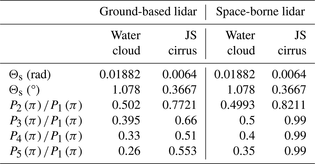
The results of this work are complementary to the data of the work by Shcherbakov et al. (2022) since most of our MC simulations were performed for the cases of (i) the same water cloud and (ii) the same jet-stream cirrus cloud. The corresponding normalized phase functions, f_W(θ) and f_JSC(θ), where θ is the scattering angle, are shown in Fig. 1 by blue and black curves, respectively; their behaviour at forward and backward angles can be seen in the insets. The scattering matrix of water cloud was computed according to the Mie theory for water spheres with the gamma size distribution, with an effective diameter of d_eff=18.0 µm (with a standard deviation of 5.3 µm). The SS characteristics of cirrus cloud were computed using the improved geometric optics method (Yang and Liou, 1996); the size distribution of particles was taken to be the gamma distribution, with d_eff=56.8 µm (with a standard deviation of 20.1 µm).

To gain a better understanding of the set of parameters that govern the MS effect, we use artificial phase functions. We use the term “chimerical” for them to underline that they are not expected to fit a real phase function but to reproduce some of its characteristics. A chimerical phase function is a sum of three Gaussian functions, G_i(θ), $i=\mathrm{1},\mathrm{2},\mathrm{3}$: a narrow peak, G₁(θ), for scattering angles close to 0° (forward direction); a somewhat smoothly varying function, G₂(θ); and a peak, G₃(π−θ), for angles close to 180°. (We use the notation π−θ in order to underline that we are dealing with the peak in the backward direction.) The first two components are in accordance with the work by Weinman (1968). The third component is inspired by the results of the work (Zhou and Yang, 2015) where rigorous numerical simulations based on solving Maxwell's equations showed that a backscattering peak exists even in cases of randomly oriented ice crystals. We use the formula $G_i\left(\mathit{\theta }\right)=a_i\cdot \exp \left[-\left({\mathit{\theta }}^{\mathrm{2}}\right)/\left({\mathit{\theta }}_{\mathrm{s},i}^{\mathrm{2}}\right)\right]$ to define the Gaussian component, G_i(θ), where θ_s,i is the $\mathrm{1}/e$ angular half width. The utility of a chimerical phase function consists of the possibility of varying one of the parameters, whereas other characteristics remain unchanged.

The first chimerical phase function, $f_{\mathrm{Ch}\mathrm{1}}\left(\mathit{\theta }\right)={\sum }_{i=\mathrm{1}}^{\mathrm{3}}{G}_i\left(\mathit{\theta }\right)$, is shown by the red curve in Fig. 1. It was designed to meet the following properties of the normalized phase function, f_W(θ), of the water cloud. f_Ch1(0)=f_W(0), f_Ch1(π)=f_W(π), and both phase functions have the same value of the lidar ratio. The width of the Gaussian component G₁(θ) of f_Ch1(θ) is assigned so that the function f_Ch1(θ)sin(θ) has the maximum at the same value of θ_max=10.82 mrad as the function f_W(θ)sin(θ) does. The width of G₃(π−θ) was adjusted so that f_Ch1(θ) and f_W(θ) lead to the coincident function R_2to1(h) (see Sect. 3.1). The width of the Gaussian component G₂(θ) is large; it ensures that a sufficient proportion of photons is scattered sideward. The chimerical phase function f_Ch2(θ) is shown by the green curve in Fig. 1. It has the same components G₁(θ) and G₂(θ) as f_Ch1(θ). The only difference is G₃(π−θ), which is larger by a factor of 15. Consequently, the curves of f_Ch1(θ) and f_Ch2(θ) coincide in Fig. 1 until the scattering angle about 170°. The values of parameters a_i and θ_s,i of the chimerical phase functions are given in Table 1.

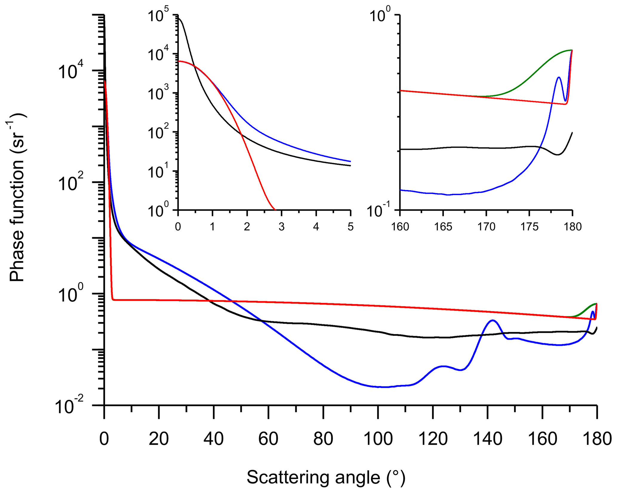
Figure 1 Normalized phase functions – water cloud: blue lines, jet-stream cirrus: black lines, chimerical phase function f_Ch1(θ): red lines, chimerical phase function f_Ch2(θ): green lines.

Table 1 Values of the input parameters of the chimerical phase functions.

Along with MC data, we provide the results, which we obtained using our code based on the Eloranta model (EM) (Eloranta, 1998) (see details in Appendix A). In what follows, the data of our simulations using the EM are referred to as multiple scattering or are labelled MS when up to five orders of scattering were considered. The contribution of the fifth order is sufficiently small in all cases considered below. The addition of the sixth order unreasonably increases the time of computing with the EM.

In this work, each cloud layer is plane-parallel (unless otherwise stated) and homogeneous. All scattering matrices were assigned an angular resolution of 0.01° (about 0.175 mrad); the emitter wavelength λ is 0.532 µm.

3 Ground-based lidar

The results of this section were obtained for a ground-based lidar, which is at the altitude of H=0 km, and the distance to the cloud base is 8 km. The full receiver field of view (RFOV) is 1.0 mrad (except in Fig. 3c and d); the full emitter field of view (EFOV) is 0.14 mrad. The emitter wavelength, λ, is 0.532 µm. (We used the characteristics of the lidar system that is in operation at Clermont-Ferrand; Freville et al., 2015.) In order to assure good statistical quality of our Monte Carlo modelling, each signal was simulated with 2×10¹¹ photons emitted by the lidar (with 4×10¹¹ photons for the cirrus clouds). Simulations of signals were performed for the orders of scattering of n=1 (single scattering) and n=2 (double scattering) and multiple scattering with an n of 20.

3.1 Single-layer cloud

The single-layer cloud is within the altitude range of H∈[8, 11] km; that is, it has an optical thickness of τ_p=3.0 (with an extinction coefficient of ε_p=1.0 km⁻¹). Black and red points in Fig. 2 show the results of our MC simulations reported in terms of the ratios R_MSto1(d) and R_2to1(d), respectively. The parameter d is the distance measured from the cloud base; i.e. the cloud is within the range of d∈[0, 3] km. The interval d∈(3, 6] km is the cloud-free molecular atmosphere – i.e. H∈(11, 14] km. Figure 2a and b correspond to the water and cirrus cloud, respectively. The relative contributions of R_MSto1(d) and R_2to1(d), computed using the EM, are shown in Fig. 2 by the green and blue curves, respectively. The MC in-cloud data – i.e. d∈[0, 3] km – were reported and discussed in the work by Shcherbakov et al. (2022). The focus of interest for this work is the cloud-free molecular atmosphere – that is, the interval of d∈(3, 6] km.

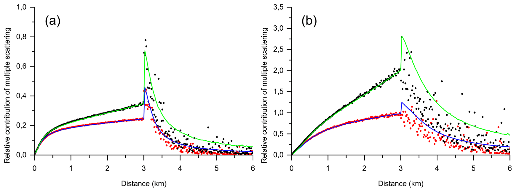
Figure 2 Monte Carlo simulations of multiple-scattering, R_MSto1 (black points), and double-scattering, R_2to1 (red points), relative contributions to lidar signals. (a) Water cloud. (b) Jet-stream cirrus. Eloranta model simulations are shown by the green (MS) and the blue (DS) curves.

Our MC simulations reveal the following features. The functions R_MSto1(d) and R_2to1(d) have undergone a stepwise jump immediately beyond the cloud far edge. It should be kept in mind that lidar signals S₁(h), S₂(h), and S_MS(h) sharply decrease immediately beyond the cloud far edge (see e.g. Fig. 7 below). The decrease of S₁(h) is faster; therefore, the ratios R_MSto1(d) and R_2to1(d) have undergone a stepwise jump. After the jump, the ratios decrease and tend to zero. It should be noted that the stepwise jump with subsequent decreasing was already reported in the work by Flesia and Starkov (1996), where multiple scattering to a space-borne lidar return from a clear molecular atmosphere obscured by transparent upper-level crystal clouds was assessed by the use of the Monte Carlo technique.

It is seen in Fig. 2a and b that the EM is able to simulate R_MSto1(d) and R_2to1(d) within the cloud layer of d∈[0, 3] km well. The simulation results can be considered acceptable in the range of d∈(3, 6] km. That is, our EM data show the stepwise jump of the same amplitude as the MC data immediately beyond the cloud far edge. In contrast, the rate of decrease of R_MSto1(d) and R_2to1(d) is lower. Therefore, the EM slightly overestimates the multiple-scattering contribution in the cloud-free molecular atmosphere. We achieved the good agreement with the MC data by adjusting the EM parameters only for the interval of d∈[0, 3] km (see details and the definition of parameters in Appendix A). We have not succeeded in improving the fitting quality for the range of d∈(3, 6] km by varying the fraction γ(h) of the energy in the forward peak of the phase function. Thus, all EM data of this work were obtained with $\mathit{\gamma }\left(h\right)=\mathrm{1}/\mathrm{2}$. The key fact is that the fittings of the water cloud case were obtained using values of the ratio $P_n\left(\mathit{\pi },h\right)/P_{\mathrm{1}}\left(\mathit{\pi },h\right),n=\mathrm{2},\mathrm{\dots },\mathrm{5}$, of about 0.5 or lower (see discussion in Appendix A). As for the cloud-free molecular atmosphere, the ratio $P_n\left(\mathit{\pi },h\right)/P_{\mathrm{1}}\left(\mathit{\pi },h\right)$ is “equal to 1.0 due to the broad nature of the molecular phase function near the backscatter direction” (Eloranta, 1998; Whiteman et al., 2001).

3.1.1 Stepwise jump and escape effect

It is of importance to underline that the discussion in this section is mainly based on the data obtained under conditions of the double-scattering (DS) approximation. Namely, the ratio R_2to1(d) of the water cloud case is used as the base to explain the stepwise jump and the escape effect for the following reasons. Both effects are well pronounced in the data for R_2to1(d) in Fig. 2a; the DS accounts for more than two-thirds of the multiple scattering; and, last but not least, the DS can be understood intuitively.

The properties of R_2to1(d) – i.e. of double scattering – within the interval d∈(3, 6] km cannot be due to the stretching of pulse length. The definition and a good explanation of the pulse stretching can be found in Miller and Stephens (1999). The simplified explanation could be as follows. In the case of double scattering, a photon goes through two scatterings within the cloud, returns to the receiver, and has the round-trip distance equal to the case of the single scattering from the range of the free atmosphere beyond the cloud far edge. The maximal round-trip distance depends on the configuration geometry – i.e. on the distance from the lidar to the cloud, the cloud depth, the EFOV, and the RFOV. In the case of Fig. 2, the EFOV and the RFOV are narrow, whereas the distance from the lidar to particles of the cloud layer is quite short. The round-trip distance of a double-scattered photon can gain a few metres in such conditions. It means that only the range of d∈(3, 3.02] km of R_2to1(d) can be somewhat affected by the pulse-length stretching. (See Fig. S1 and the explanation in the Supplement.) In addition, we have to underline the following. The EM uses the assumption that “the multiply scattered photons are scattered from the same slab as the single-scattered photons” (see p. 2466 in Eloranta, 1998). To put it differently, the EM ignores the pulse stretching. Nevertheless, it reproduces, with good accuracy, the stepwise jumps in Fig. 2 on the basis of the phase-function parameters. Therefore, it is safe to assume that the stepwise jump of R_MSto1(d) and R_2to1(d) is due to the stepwise jump in phase-function properties at angles close to 180° (between the phase function of particles within the cloud and the Rayleigh scattering within the free atmosphere).

That assumption is confirmed by the plots in Fig. 3a and b, where the results of MC simulations are shown as the ratios R_MSto1(d) and R_2to1(d) for the cases of the chimerical phase functions f_Ch1(θ) and f_Ch2(θ), respectively. We adjusted the width of the component G₃(π−θ) of f_Ch1(θ) so that MC simulations with f_Ch1(θ) give the same R_2to1(d) within the range of d∈[0, 3] km as R_2to1(d) of the water cloud in Fig. 2a. It turns out that the peak in the backward direction of the water cloud is a little bit larger than G₃(π−θ) of f_Ch1(θ) (see Fig. 1). Nevertheless, the MC data in Fig. 3a are coincident with the MC data in Fig. 2a for the ratios R_MSto1(d) and R_2to1(d) within the full range of d∈[0, 6] km. The good agreement is due to the fact that one of the key parameters of multiple scattering is a weighted average of a phase function near the backscatter direction (see Eq. 10 of Eloranta, 1998; see Fig. S2 and the intuitive explanation in the Supplement). That average depends on the properties of the forward and backward peaks of the phase function and on the receiver field of view. This means that we fitted the value of the weighted average when we adjusted the width of the Gaussian function G₃(π−θ).

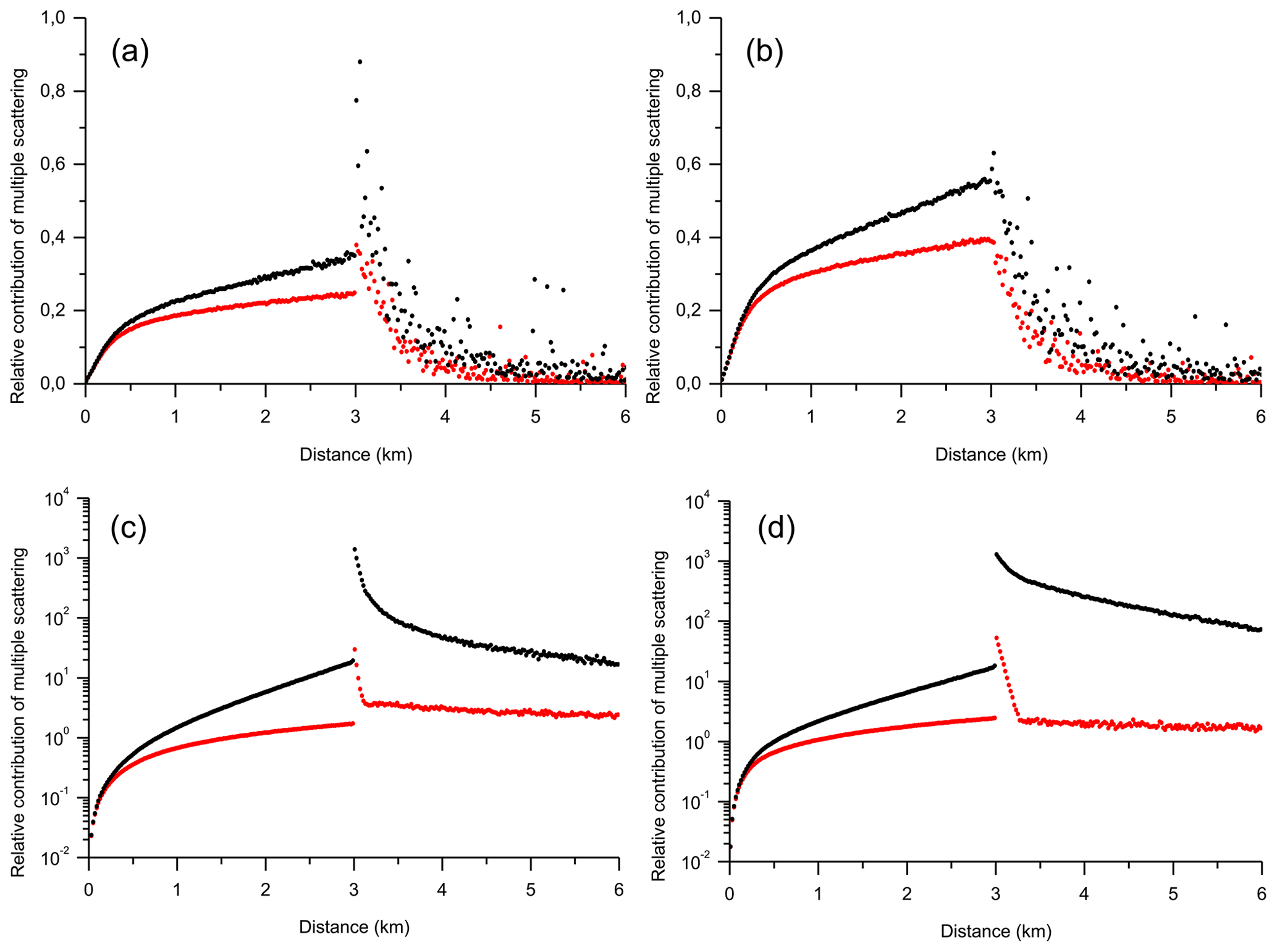
Figure 3 Monte Carlo simulations of multiple-scattering, R_MSto1 (black points), and double-scattering, R_2to1 (red points), relative contributions to lidar signals. In panels (a) and (b), RFOV = 1 mrad. In panels (c) and (d), RFOV = 110 mrad. (a) Chimerical phase function f_Ch1(θ). Panels (b) and (d) show the chimerical phase function f_Ch2(θ). (c) Water cloud.

The chimerical phase functions, f_Ch1(θ) and f_Ch2(θ), have the same values of the parameters θ_s,1 and θ_s,2, but the width θ_s,3 is 15 times higher for f_Ch2(θ). That leads to marked distinctions in the ratios R_MSto1(d) and R_2to1(d) (see Fig. 3b). There is no stepwise jump immediately beyond the cloud far edge. It means that the component G₃(π−θ) of f_Ch2(θ) is large enough to have the weighted average equal to f_Ch2(π), as in the case of the Rayleigh phase function. If we use the terms of the Eloranta model (Eloranta, 1998), the ratio $P_{\mathrm{2}}\left(\mathit{\pi },h\right)/P_{\mathrm{1}}\left(\mathit{\pi },h\right)=\mathrm{1}$ for the phase function f_Ch2(θ) – i.e. it has the same value as in the case of the Rayleigh phase function. To put it differently, a higher proportion of photons are scattered by the cloud in the backward direction within the RFOV and contributes to lidar signals in the MS case and under the DS approximation. As a consequence, the ratios R_MSto1(d) and R_2to1(d) of Fig. 3b are much higher than in Figs. 2a and 3a for the in-cloud range of d∈[0, 3] km.

The MC data of Figs. 2a and 3a, b are coincident within the interval of the cloud-free molecular atmosphere, d∈(3, 6] km, if they are superimposed in the same figure. Thus, it is safe to assume that the following two properties are defined by the forward-peak width of the phase function and the RFOV: (i) the proportion of scattered photons emerging from a cloud that are subsequently scattered in the backward direction to the receiver and (ii) the rate of decrease of the relative contribution of multiple scattering outside the cloud. (We recall that we are dealing with ground-based lidar, the cloud optical thickness is not high, and the RFOV and the EFOV are narrow.) That assumption explains the difference in the rates of decrease within the range of d∈[3, 6] km between Fig. 2a and Fig. b. The forward peak of the scattering phase function of the cirrus cloud is much stronger compared to the one of the water cloud. That leads to the slower rate of decrease.

In our opinion, those properties are a direct consequence of the fact that the photons scattered within the forward peak escape the sampling volume. (For the sake of simplicity, we will use the term “escape effect” to refer to that phenomenon.) The following arguments justify that statement. Let us consider the case of the forward scattering. If we refer to Fraunhofer diffraction by large spheres (see e.g. Chap. 8.3 of Van de Hulst, 1981), the first dark ring – i.e. the Airy disc – is at the angle of θ_Airy≈36 mrad (about 2°) when a particle has a diameter of 18 µm and a wavelength, λ, of 0.532 µm (${\mathit{\theta }}_{\mathrm{Airy}}\gg \mathrm{RFOV}/\mathrm{2}=\mathrm{0.5}$ mrad). If we refer to the phase function of the water cloud (see Fig. 1), the intervals of the angles of [0, 0.5] mrad and [0, 36] mrad account for 0.059 % and 41.3 % of the total scattered light, respectively. In such conditions, it can hardly be expected that a large proportion of small-angle forward-scattered photons always remain within the field of view of the detector; what is more likely is that photons escape the sampling volume.

With the aim of confirming our arguments, we performed MC simulations for the cases of larger RFOVs. All but the RFOV parameters of lidar configuration and the water cloud properties are the same as in the case of Fig. 2a. The full RFOV is 110 mrad. Such a large value ensures that the narrow peak G₁(θ) (forward direction) of the chimerical phase functions is completely within the angle of $\mathrm{RFOV}/\mathrm{2}=\mathrm{55}$ mrad (about 3°). Black and red points in Fig. 3c and d show the results of our MC simulations reported in terms of the ratios R_MSto1(d) and R_2to1(d), respectively. Figure 3c and d show the cases of the water cloud and the chimerical phase function f_Ch2(θ), respectively. (Note the log scale on the y axis in Fig. 3c and d.)

It is seen that the ratios R_2to1(d) have undergone a very strong stepwise jump immediately beyond the cloud far edge. If we consider the configuration geometry – i.e. the angle of $\mathrm{RFOV}/\mathrm{2}=\mathrm{55}$ mrad – and the distance from the lidar to the cloud far edge of 11 km, the pulse stretching is the cause of the jump. The pulse stretching strongly affects R_2to1(d) in Fig. 3d within the range of d∈(3, 3.25] km. The ratio R_2to1(d) is almost constant within the interval of d∈[3.25, 6] km. (In our opinion, the slight decrease is due to the pulse-stretching effect.) The properties of the ratio R_2to1(d) in Fig. 3c are the same but less pronounced. We can hypothesize that photons that were forward-scattered within angles of > 3° play a noticeable role in the case of the water cloud. The results shown in Fig. 3c and d mean that only when the RFOV is sufficiently large do small-angle forward-scattered photons remain within the field of view of the detector, and the escape effect is eliminated. As for the cases of multiple scattering, the ratios R_MSto1(d) in Fig. 3c and d are very high due to the large RFOV, and the escape effect is evident.

It is seen that the decrease due to the escape effect is an inherent part of R_MSto1(d) properties within the free atmosphere beyond the cloud far edge. That property is in direct contradiction with Eqs. (10)–(14) above, which are the consequences of Eq. (5). Therefore, we can conclude that Eq. (5) is an approximate model of lidar signals under MS conditions because it does not take into account the escape effect.

3.1.2 Practical aspects

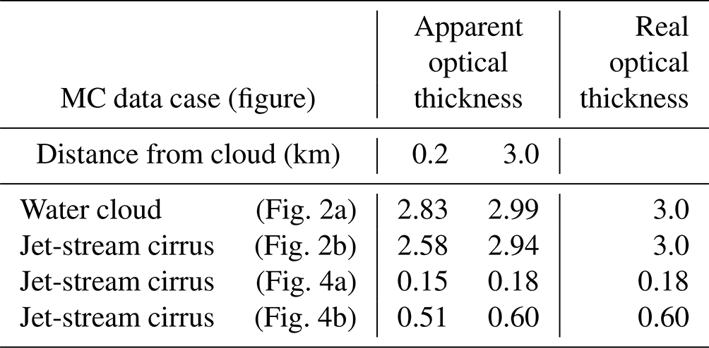
Knowing that the value of the extinction coefficient of ε_p=1.0 km⁻¹ is not typical of cirrus clouds, we provide practitioners with estimations of MS effects for lower values of ε_p of the jet-stream cirrus. Black points in Fig. 4 show the results of our MC simulations reported in terms of the ratio R_MSto1(d). The parameter d is the distance measured from the cloud base – i.e. the cloud is within the range of d∈[0, 3] km. The interval of d∈(3, 6] km is the cloud-free molecular atmosphere – i.e. the altitude of H∈(11, 14] km. The MC simulations were performed for the same geometry of plane-parallel homogeneous cloud as in the case of Fig. 2b. The only difference consists of the values of the extinction coefficient, which were ε_p=0.06 and ε_p=0.2 km⁻¹ in Fig. 4a and b, respectively. It is seen that the lidar data are affected by MS within the cloud (d∈[0, 3] km) and above the cloud far edge (d∈(3, 6] km). The cases in Fig. 4 are characterized by the quite low values of the extinction coefficient – i.e. the low probability of the interaction of a photon with cloud particles. Moreover, the RFOV – i.e. the sampling volume – and the forward peak of the scattering phase function are narrow. All that led to the rather high dispersion of the MC data in Fig. 4 despite the very high number, 4×10¹¹, of sampled photons. Nevertheless, it is safe to conclude that the MS contribution decreases with the distance from the cloud far edge due to the escape effect. The MS contribution is lower than 5 % within the regions of the cloud-free molecular atmosphere, with the distance from the cloud far edge of about 1 km or higher when ε_p≤0.2 km⁻¹.

Table 2 shows the values of the apparent optical thickness, $\mathit{\eta }\cdot {\mathit{\tau }}_{\mathrm{p}}\left(h_{\mathrm{b}},h_{\mathrm{end}}\right)$, of the cloud computed using Eq. (13) with two values of h₂ assigned within the interval of d∈(3, 6] km (with an altitude of H∈(11, 14] km). The values of 0.2 and 3.0 km mean the distance from the cloud far edge within the cloud-free molecular atmosphere; they correspond to d=3.2 km (H=11.2 km) and d=6.0 km (H=14.0 km), respectively. It is seen that the computed value of the apparent optical thickness depends on the chosen value of h₂. It is close to the value of the real optical thickness, when h₂=14.0 km, and can be about 15 % lower, when h₂=11.2 km, in the cases of the jet-stream cirrus.

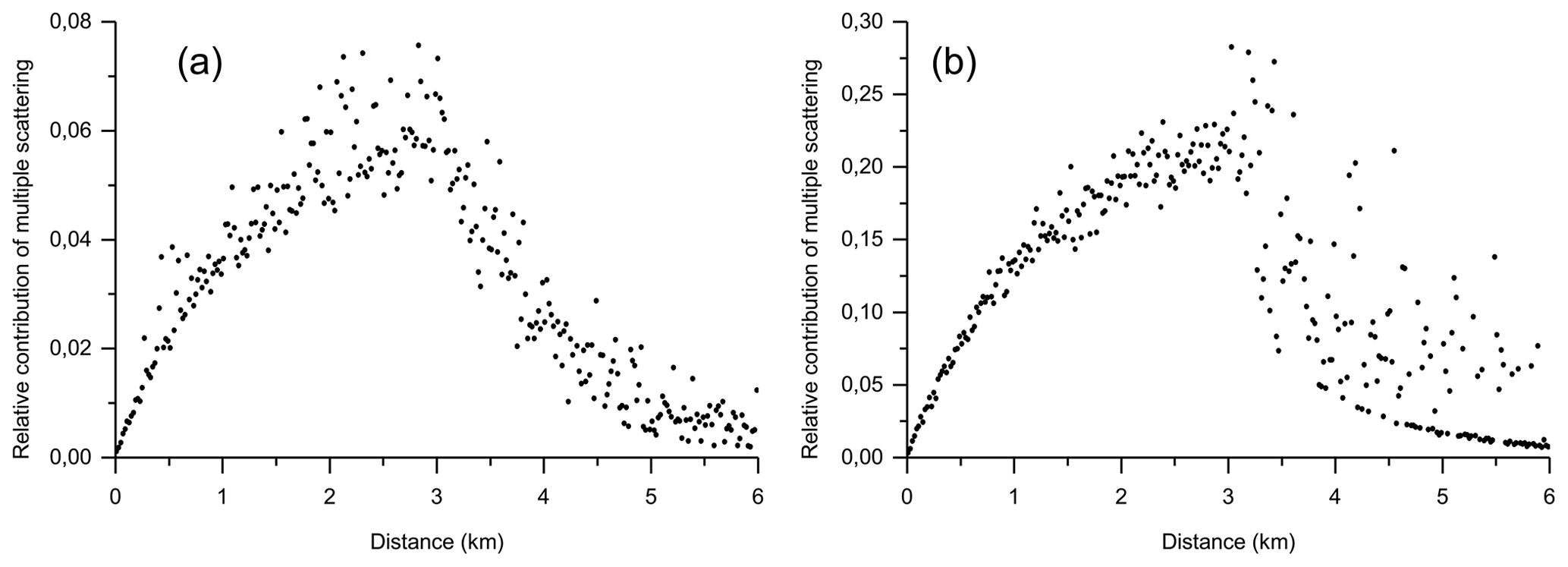
Figure 4 Monte Carlo simulations of multiple-scattering relative contributions, R_MSto1, to lidar signals from the jet-stream cirrus; the extinction coefficients are (a) 0.06 km⁻¹ and (b) 0.2 km⁻¹.

Table 2 Estimated values of the apparent optical thickness, $\mathit{\eta }\cdot {\mathit{\tau }}_{\mathrm{p}}\left(h_{\mathrm{b}},h_{\mathrm{end}}\right)$.

3.2 Two-layered cloud

The two-layered cloud consists of homogeneous layers situated at the altitudes from 8 to 9 km and from 10 to 11 km. Every layer has the optical thickness of τ_p=1.0; the total optical thickness is τ_p=2.0. The black and red points in Fig. 5 show the results of our MC simulations reported in terms of the ratios R_MSto1(d) and R_2to1(d), respectively. The parameter d is the distance measured from the cloud base; i.e. the layers are within the ranges of d∈[0, 1] and d∈[2, 3] km. The intervals of d∈(1, 2) and d∈(3, 6] km are the cloud-free molecular atmosphere. Figure 5a and b correspond to the water and cirrus cloud, respectively. The relative contributions R_MSto1(d) and R_2to1(d) computed using the EM are shown in Fig. 5 by green and blue lines, respectively.

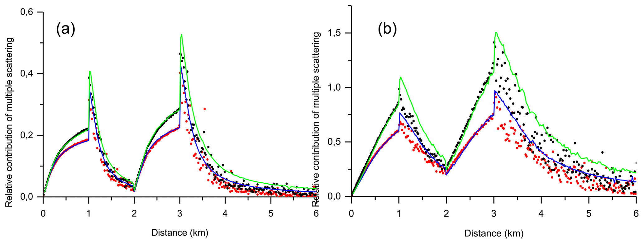
Figure 5 Monte Carlo simulations of multiple-scattering, R_MSto1 (black points), and double-scattering, R_2to1 (red points), relative contributions to lidar signals. (a) Water cloud. (b) Jet-stream cirrus. Eloranta model simulations are shown by the green (MS) and the blue (DS) curves.

The features of the MC data within the intervals of the cloud-free molecular atmosphere are closely similar to those addressed in the previous section. In addition, the following property is noteworthy. The rate of decrease of the MS relative contributions in the case of the water cloud is quite fast; therefore, scattered photons emerging from the first layer almost do not affect the lidar signal from the second layer. (The values of the ratios R_MSto1(d=2.0) and R_2to1(d=2.0) are close to zero.) As it was discussed above, the rate of decrease of the MS relative contributions in the case of the cirrus clouds is much slower compared to the water cloud case. Therefore, scattered photons emerging from the first layer affect the lidar signal from the second layer so that the ratios R_MSto1(d=2.0) and R_2to1(d=2.0) are about 0.25. In other words, the lidar signal from the near edge of the second layer is about 25 % higher compared to the SS approximation. Obviously, the distance between cloud layers is a key parameter. The values of the ratios R_MSto1(d) and R_2to1(d) at the near edge of the second layer vary if that distance changes.

As for our EM simulations, we used the same values of the ratio $P_n\left(\mathit{\pi },h\right)/P_{\mathrm{1}}\left(\mathit{\pi },h\right),n=\mathrm{2},\mathrm{\dots },\mathrm{5}$, as in the previous section for each cloud layer. We can conclude one more time that the EM is able to simulate MS contributions within the cloud layers well. As for the intervals of the cloud-free molecular atmosphere, the behaviour of R_MSto1(d) and R_2to1(d) is correct, whereas the MS contribution is slightly overestimated.

4 Space-borne lidar

The results of this section were obtained for a space-borne lidar, which is at an altitude of H=705 km. The full receiver field of view (RFOV) is 0.13 mrad; the full emitter field of view (EFOV) is 0.1 mrad. The emitter wavelength, λ, is 0.532 µm. Those values correspond to the technical characteristics of the Cloud-Aerosol Lidar with Orthogonal Polarization (CALIOP) (Young and Vaughan, 2009). In order to assure good statistical quality of our Monte Carlo modelling, each signal was simulated with 2×10¹¹ photons emitted by the lidar (with 4×10¹¹ photons for the cirrus clouds). Simulations of signals were performed for the orders of scattering of n=1 (single scattering) and n=2 (double scattering) and multiple scattering with an n of 20.

4.1 Single-layer cloud

4.1.1 Plane-parallel homogeneous cloud

The single-layer cloud is within the altitude range of $H\in [\mathrm{8},\mathrm{11}]$ km and has an optical thickness of τ_p=3.0 (with an extinction coefficient of ε_p(h)=1.0 km⁻¹). For reasons of direct comparison of our data with those addressed in the literature, we show our simulated signals of the space-borne lidar in Fig. 6. The SS S₁(h) and MS S_MS(h) lidar signals are shown by the blue and black points, respectively. Qualitatively, Fig. 6a and b are similar to Fig. B1c and d, respectively, of the work by Reverdy et al. (2015) and to Fig. 1c and d of the work by Donovan (2016). The distinction in the quantitative characteristics is due to the difference in the cloud optical thickness and optical parameters of the particles. The feature that the MS signals below the cloud base tend to the SS signals is well pronounced. Multiple-scattering ratio R_MSto1(d) is more suitable to quantify that feature compared to lidar signals shown in the semi-logarithmic plot.

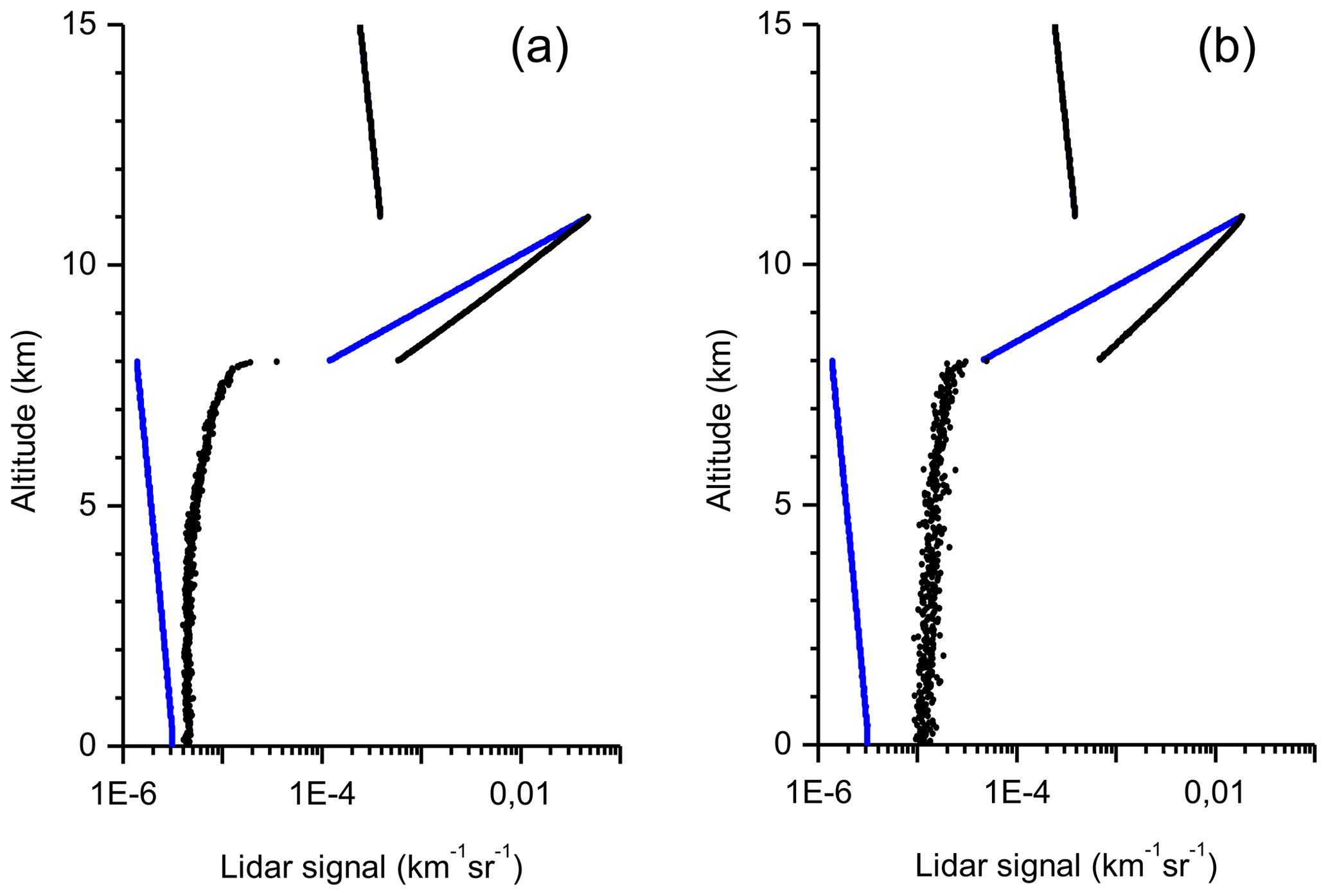
Figure 6 Monte Carlo simulations of single-scattering (blue points) and multiple-scattering (black points) lidar signals. (a) Water cloud. (b) Jet-stream cirrus.

Black and red points in Fig. 7 show the results of our MC simulations reported in terms of the ratios R_MSto1(d) and R_2to1(d), respectively. The parameter d is the distance measured from the cloud near edge to the lidar – i.e. the cloud is within the range of d∈[0, 3] km. (d=0 km corresponds to an altitude of H=11 km.) The interval of d∈(3, 11] km (an altitude, H, from 8 to 0 km) is the cloud-free molecular atmosphere below the cloud. Figure 7a and b correspond to the water and cirrus cloud, respectively. The relative contributions R_MSto1(d) and R_2to1(d) computed using the EM are shown in Fig. 7 by the green and blue curves, respectively. The MC in-cloud data – i.e. d∈[0, 3] km – were reported and discussed in the work by Shcherbakov et al. (2022). The focus of interest for this work is the cloud-free molecular atmosphere – that is, the interval of d∈(3, 11] km.

The features of the MC data within the range of the cloud-free molecular atmosphere have a lot in common with those addressed in Sect. 3.1. In addition, the following properties are noteworthy. In the case of the space-borne lidar, the difference between values of R_MSto1(d) and R_2to1(d) is much larger compared to Fig. 2a and b; that is, the third and higher orders of scattering dominate. The escape effect does affect the lidar signals. At the same time, the rate of decrease of R_MSto1(d) and R_2to1(d) is much slower. The distance of 8 km from the cloud is not sufficient for reaching the conditions of the SS approximation. That result is of importance for practitioners who work with data of space-borne lidars because the estimated value of the apparent optical thickness depends on the distance from the cloud far edge chosen as the reference point h₂ (see details in Sect. 4.1.3).

As in the cases of the ground-based lidar, the EM is able to simulate MS contributions within the cloud layers well. We employed the same approach to obtain values of the ratio $P_n\left(\mathit{\pi },h\right)/P_{\mathrm{1}}\left(\mathit{\pi },h\right),n=\mathrm{2},\mathrm{\dots },\mathrm{5}$, as in Sect. 3.1 (see Appendix A for details). As in the cases of the ground-based lidar, the fittings of the water cloud case were obtained using values of the ratios $P_n\left(\mathit{\pi },h\right)/P_{\mathrm{1}}\left(\mathit{\pi },h\right),n=\mathrm{2},\mathrm{\dots },\mathrm{5}$, about 0.5 or lower. The behaviours of R_MSto1(d) and R_2to1(d) are correct within the range of the cloud-free molecular atmosphere, whereas the MS contribution is slightly overestimated. It is seen that the EM is not able to reproduce the amplitude of the stepwise jump of R_MSto1(d) immediately beyond the cloud far edge. Thus, the stepwise jump in those cases is not only due to the stepwise jump in phase-function properties for angles close to 180°. We can suggest that the range of d∈(3, 3.1] km is somewhat affected by the pulse stretching.

Figure 7 Monte Carlo simulations of multiple-scattering, R_MSto1 (black points), and double-scattering, R_2to1 (red points), relative contributions to lidar signals. (a) Water cloud. (b) Jet-stream cirrus. Eloranta model simulations are shown by the green (MS) and the blue (DS) curves.

4.1.2 Non-uniform beam filling

Another problem associated with a reference range taken below the cloud base consists of the following. Space-borne lidars such as CALIOP have a quite large laser footprint so that a cloud field can be horizontally heterogeneous within the footprint. That raises the well-known problem of the non-uniform beam filling (NUBF). Some effects of the NUBF on lidar data within cloud fields were addressed in other works (Szczap et al., 2021; Alkasem et al., 2017). The lidar signals from the cloud-free atmosphere below the cloud base are affected as well.

In order to understand some basic properties under 3D multiple-scattering conditions, we performed simulations for the case of a very simple 3D field. (All data of this subsection were obtained using the McRALI software – i.e. the Monte Carlo method.) A homogeneous cloud covers half of the field, when viewed from the top. The centre of the CALIOP laser footprint is exactly on the cloud border. In other words, half of the laser beam passes through the cloud, and the other half goes through the molecular atmosphere. The thickness of the cloud is 3 km, and the cloud top altitude is 11 km. The extinction coefficient of the particles of the cloud is 2 km⁻¹. To put it differently, we have chosen the value of the extinction coefficient so that the amount of particles within the volume bounded by the EFOV in the 3D case is exactly the same as in the case of the plane-parallel homogeneous cloud. The same is true if we consider the sampling volume. Therefore, the optical thickness of the 3D cloud, when averaged over the EFOV, is $\mathrm{3}=\left(\mathrm{0}+\mathrm{6}\right)/\mathrm{2}$.

The NUBF effect is so high in such conditions that it has to be shown in terms of lidar signals. Figure 8 is complementary to Fig. 7; i.e. it shows the results based on the same MC simulations but as the lidar signals. Figure 8a and b correspond to the water and cirrus cloud, respectively. The black and red lines are lidar signals (corrected for the offset and instrumental factors) obtained with the Monte Carlo method in MS conditions and the SS approximation, respectively. We recall that the black and red lines were obtained for the case of the homogeneous plane-parallel cloud with an optical thickness of τ_p=3.0.

The green lines in Fig. 8 are the lidar signals computed in the case of the 3D cloud field in MS conditions. Within the in-cloud altitude range of H∈[8, 11] km, they are lower than the MS signals from the corresponding homogeneous cloud (the black lines), which is in total agreement with the theory (see Chap. 3.1 in Alkasem et al., 2017). As for the range below the cloud base, it is seen that the NUBF makes the situation much more aggravated. The lidar signals (the green curves) are around 200 times higher compared to the SS approximation for the homogeneous plane-parallel cloud (the red curves). That is the direct consequence of the fact that in the 3D case, half of the laser beam passes through the molecular atmosphere, whereas the other half passes through the cloud with 2τ_p=6.

Figure 8 Monte Carlo simulations of lidar signals. Homogeneous plane-parallel cloud: black curves correspond to multiple-scattering and red curves correspond to single-scattering conditions; green curves correspond to multiple scattering in the 3D cloud field. (a) Water cloud. (b) Jet-stream cirrus.

4.1.3 Practical aspects

Knowing that the value of the extinction coefficient of ε_p=1.0 km⁻¹ is not typical of cirrus clouds, we provide practitioners with estimations of the escape and NUBF effects for lower values of ε_p of the jet-stream cirrus. The black points in Fig. 9 show the values of the MS relative contribution, R_MSto1(d) (see Eq. 3), in the case of the homogeneous plane-parallel cloud. The MC simulations were performed for the same geometry of plane-parallel homogeneous cloud as in the case of Fig. 7b. The only difference consists of the values of the extinction coefficient, which were ε_p=0.06 and ε_p=0.2 km⁻¹ in Fig. 9a and b, respectively. It is seen that the lidar data are affected by MS within the cloud (d∈[0, 3] km) and below the cloud base (d∈(3, 11] km).

NUBF effects are shown by the red points in Fig. 9. As previously, (i) a homogeneous cloud covers half of the field, when viewed from the top; (ii) the centre of the CALIOP laser footprint is exactly on the cloud border; and (iii) the value of ε_p is a factor of 2 higher than the extinction coefficient of the corresponding plane-parallel cloud. The values of the extinction coefficient of the 3D cloud, when averaged over the EFOV, are $\mathrm{0.06}=\left(\mathrm{0}+\mathrm{0.12}\right)/\mathrm{2}$ and $\mathrm{0.2}=\left(\mathrm{0}+\mathrm{0.4}\right)/\mathrm{2}$ in the cases of Fig. 9a and b, respectively. The relative difference

$$\begin{array}{}\text{(15)}& R_{\mathrm{NUBFto}\mathrm{1}}\left(h\right)=\left[S_{\mathrm{NUBF}}\left(h\right)-S_{\mathrm{1}}\left(h\right)\right]/S_{\mathrm{1}}\left(h\right)\end{array}$$

is taken to be a measure of the NUBF effects, where S_NUBF(h) is the MS lidar signal simulated using the Monte Carlo method in the case of the 3D cloud field and S₁(h) is the lidar signal computed in the case of the corresponding plane-parallel cloud under the SS approximation. In other words, the parameter R_NUBFto1 is devoted to showing the relative contribution of the MS and the NUBF taken together.

Figure 9 Monte Carlo simulations of multiple-scattering effects (jet-stream cirrus). Black points are the relative contributions, R_MSto1, to lidar signals from a homogeneous plane-parallel cloud; red points are the relative contributions, R_NUBFto1, of the MS and the NUBF to lidar signals from a 3D cloud. The extinction coefficients are (a) 0.06 km⁻¹ and (b) 0.2 km⁻¹.

At another time, it is seen that the MS effect is somewhat weakened by the NUBF within the cloud range (d∈[0, 3] km). When the optical thickness within the cirrus cloud is quite low, MS lidar signals from a 3D cloud are fairly close to the SS lidar signals from the corresponding plane-parallel homogeneous cloud (see Figs. 8b and 9). That property is not valid in the case of the water cloud (see Fig. 8a). It can be hypothesized that more photons escape through the cloud side when the forward-scattering peak of the particles is larger.

As for lidar signals within the range of the free atmosphere below the cloud base (d∈(3, 11] km), they are always affected either by the multiple scattering or by the non-uniform beam filling. There is no interval where the MS effect is lower than 5 %. Also, the NUBF effect on lidar signals is always higher than the MS effect in the case of plane-parallel cloud. We recall that our comparison is made on the condition that the number of particles within the volume bounded by the EFOV in the 3D case is exactly the same as in the case of the plane-parallel homogeneous cloud.

Table 3 Estimated values of the apparent optical thickness, $\mathit{\eta }\cdot {\mathit{\tau }}_{\mathrm{p}}\left(h_{\mathrm{b}},h_{\mathrm{end}}\right)$. The real optical thickness of 3D clouds is the value averaged over the EFOV.

The escape effect is noteworthy as well. It is seen that R_MSto1(d) and R_NUBFto1(d) decrease with the increasing distance from the cloud base in all four cases of Fig. 9. Examples of its consequences in terms of the apparent optical thickness of the cloud, $\mathit{\eta }\cdot {\mathit{\tau }}_{\mathrm{p}}\left(h_{\mathrm{b}},h_{\mathrm{end}}\right)$, are given in Table 3. The data were computed using Eq. (13), with two values of h₂ assigned within the interval of d∈(3, 11] km (with an altitude of H∈(8, 0] km). The values 0.2 and 7.98 km mean the distance from the cloud far edge within the cloud-free molecular atmosphere; they correspond to d=3.2 (H=7.8) and d=10.98 (H=0.02) km, respectively. It is seen that the estimated values of $\mathit{\eta }\cdot {\mathit{\tau }}_{\mathrm{p}}\left(h_{\mathrm{b}},h_{\mathrm{end}}\right)$ are always lower than the values of the real optical thickness; they are much lower in the cases of the 3D cloud (NUBF) compared to the plane-parallel cloud, and they strongly depend on the assigned value of h₂.

As in the case of the ground-based lidar, we can conclude that Eq. (5) does not take into account the escape effect. Therefore, it is only an approximate model of MS signals from space-based lidars.

4.2 Two-layered cloud

The two-layered cloud is the same as in Sect. 3.2 – that is, two homogeneous layers are at altitudes from 8 to 9 km and from 10 to 11 km. Every layer has an optical thickness of τ_p=1.0; the total optical thickness is τ_p=2.0. The black and red points in Fig. 10 show the results of our MC simulations reported in terms of the ratios R_MSto1(d) and R_2to1(d), respectively. The parameter d is the distance measured from the cloud near edge – i.e. d=0 km corresponds to an altitude of H=11 km. The cloud layers are within the ranges of d∈[0, 1] and d∈[2, 3] km. The intervals of d∈(1, 2) and d∈(3, 11] km (with altitudes, H, from 10 to 9 km and from 8 to 0 km) are the cloud-free molecular atmosphere. Figure 10a and b correspond to the water and cirrus cloud, respectively.

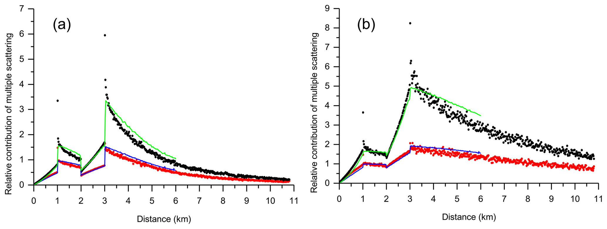
Figure 10 Monte Carlo simulations of multiple-scattering, R_MSto1 (black points), and double-scattering, R_2to1 (red points), relative contributions to lidar signals. (a) Water cloud. (b) Jet-stream cirrus. Eloranta model simulations are shown by the green (MS) and the blue (DS) curves.

The main properties of our MC simulations in Fig. 10 are in agreement with the results of the work by Flesia and Starkov (1996); the distinctions are due to differences in the phase functions and the configuration characteristics. In addition, the vertical resolution in our work is 7.5 times better, and, therefore, the ratios R_MSto1(d) and R_2to1(d) are seen in more detail.

The general behaviour of MC data around d=1 km and within the range of d≥3 km in Fig. 10 is the same as it is within the range of d≥3 km in Fig. 7. Thus, we focus attention only on the interval around d=2 km – that is, on the near edge of the second cloud layer. The difference between the cases of the ground-based and the space-borne lidars is better seen from comparison of Figs. 5a and 10a, i.e. the water clouds. In the case of the space-borne lidar, the sampling volume is so large (due to the large receiver footprint) that the majority of forward-scattered photons remain within it. This leads to the value R_MSto1(d=2.0 km), which is almost the same as R_MSto1(d=1.0 km) (see Fig. 10a). In contrast, the sampling volume, i.e. the footprint, is narrow in the case of the ground-based lidar. The majority of forward-scattered photons escape it when they are going through the cloud-free molecular atmosphere within the interval d∈(1, 2) km. This leads to the value R_MSto1(d=2.0 km) close to zero (see Fig. 5a). Generally, the same features are observed in Figs. 5b and 10b. They are less pronounced because the forward-scattering peak of the phase function of cirrus cloud is much narrower.

The relative contributions R_MSto1(d) and R_2to1(d) computed using the EM are shown in Fig. 10 by green and blue curves, respectively. The simulations were performed with the same values of the ratio $P_n\left(\mathit{\pi },h\right)/P_{\mathrm{1}}\left(\mathit{\pi },h\right),n=\mathrm{2},\mathrm{\dots },\mathrm{5}$, as in Sect. 4.1.1. Generally, the EM curves follow the MC results well. It is seen another time that the EM slightly overestimates the MS contribution in the cloud-free intervals and it is not able to reproduce the effect related to the pulse stretching.

5 Conclusions

We performed Monte Carlo simulations of single-wavelength lidar signals from multi-layered clouds with special attention focused on features of the multiple-scattering (MS) effect in regions of the cloud-free molecular atmosphere, i.e. between layers or outside a cloud system. Despite the fact that the strength of lidar signals from molecular atmosphere is much lower compared to the in-cloud intervals, studies of MS effects in such regions are of interest from scientific and practical points of view. The results of this work are shown and discussed in terms of relative contributions of multiple scattering, that is, multiple-to-single-scattering lidar return ratios R_MSto1(d). That provides the possibility of accentuating the visibility of MS effects.

The scattered photons emerging from a cloud do affect lidar signals received from the intervals of the cloud-free molecular atmosphere. The MS effect is rather high within the region that is close to the far edge of a cloud. Those high values of the ratios R_MSto1(d) are due to the features of the molecular backscattering, i.e. to the fact that the ratios $P_n\left(\mathit{\pi },h\right)/P_{\mathrm{1}}\left(\mathit{\pi },h\right)$ are “equal to 1.0 due to the broad nature of the molecular phase function near the backscatter direction” (Whiteman et al., 2001; Eloranta, 1998). In the cases of the space-borne lidar, the additional MS contribution is due to the pulse stretching.

The MS effect on lidar signals decreases with the increasing distance from the cloud far edge; i.e. the ratio R_MSto1(d) tends to zero. The decrease is the direct consequence of the fact that the forward peak of particle phase functions is much larger than the receiver field of view. Therefore, the photons scattered within the forward peak escape the sampling volume formed by the RFOV – i.e. the escape effect. The escape effect is an inherent part of MS properties within the free atmosphere beyond the cloud far edge. That property is in direct contradiction with Eq. (5). Consequently, Eq. (5) is an approximate model of lidar signals under MS conditions.

The two-way transmittance method (see e.g. Young and Vaughan, 2009; Giannakaki et al., 2007) is based on Eq. (5) and used to deduce the values of the apparent optical thickness of clouds. In view of the results of this work, it is advisable at least to choose the reference point always at the same distance from the cloud far edge when estimating the apparent optical thickness of clouds.

In the cases of the ground-based lidar, the MS contribution is lower than 5 % within the regions of the cloud-free molecular atmosphere, with the distance from the cloud far edge of about 1 km or higher. Therefore, it is safe to say that practitioners can use those regions as a reference and estimate the real optical thickness of clouds (see e.g. Giannakaki et al., 2007, and references therein) if the EFOV and the RFOV are not very large. In the cases of the space-borne lidar, the rate of decrease of the MS contribution is so slow that the threshold of 5 % can hardly be reached.

Using an example of a very simple 3D field, we demonstrated that the effect of non-uniform beam filling can be extremely strong in the case of a space-borne lidar. It is so strong that, in our opinion, practitioners should employ, with proper precautions, lidar data from regions below the cloud base, when treating data from a space-borne lidar. At the same time, it should be underlined that the effects of the NUBF need further study, which will provide statistically significant results.

In the case of two-layered cloud, the distance of 1 km is sufficiently large so that the scattered photons that emerge from the first layer do not affect signals from the second layer when we are dealing with the ground-based lidar. In contrast, signals from the near edge of the second cloud layer are severely affected by the photons emerging from the first layer in the case of a space-borne lidar.

We evaluate the Eloranta model (EM) (Eloranta, 1998) in extreme conditions and show its good performance in the cases of ground-based and space-borne (CALIOP) lidars. When the extinction coefficient is about 1.0 km⁻¹ or lower, and the EFOV and the RFOV are quite narrow, five orders of scattering are sufficient for obtaining satisfying accuracy of the simulations. At the same time, we revealed the shortcoming that affects practical applications of the EM. Namely, values of the key parameters, i.e. of the ratio $P_n\left(\mathit{\pi },h\right)/P_{\mathrm{1}}\left(\mathit{\pi },h\right)$ of phase functions in the backscatter direction for the nth-order-scattered photon and a singly scattered photon, depend not only on the particle phase function but also on the distance from a lidar to the cloud and the receiver field of view. Values of the ratio $P_n\left(\mathit{\pi },h\right)/P_{\mathrm{1}}\left(\mathit{\pi },h\right)$ vary within a quite large range. Therefore, the multiple-scattering contribution to lidar signals can be largely overestimated or underestimated if erroneous values of the ratios are assigned to the EM. That problem can be circumvented using Monte Carlo simulations or the empirical model (Shcherbakov et al., 2022) to calibrate the ratio $P_n\left(\mathit{\pi },h\right)/P_{\mathrm{1}}\left(\mathit{\pi },h\right)$.

Appendix A: Input parameters of the Eloranta model in homogeneous-cloud conditions

A1 Eloranta model

We have chosen to evaluate the Eloranta model (EM) (Eloranta, 1998) due to its following attractive features. The input parameters have a clear physical meaning. The contribution of each of the n orders of scattering can be computed separately. The corresponding code can be developed without much difficulty because multiple integrals are the core of the EM. The good performance of the Eloranta model (EM) (Eloranta, 1998) in homogeneous-cloud conditions has already been reported in the literature (see e.g. Eloranta, 1998; Donovan and Van Lammeren, 2001). In our opinion, our results above demonstrate the reliability of the EM in extreme conditions – i.e. when the extinction coefficient has undergone a stepwise jump. The objective of this appendix is to reveal some significant features of the EM's input parameters that are related to the particle phase function.

We developed two versions of the code based on the EM. The first version corresponds to Eq. (8) of Eloranta (1998). In order to avoid ambiguity, we rewrite that equation in a way that all functions, including ε(x), γ(x), and Θ_s(x), are assigned in the coordinate system where the lidar is at h=0 and h is the distance from the lidar:

$$\begin{array}{}\text{(A1)}& \begin{array}{rl}& R_{\mathrm{nto}\mathrm{1}}\left(h\right)={\displaystyle \frac{P_n\left(\mathit{\pi },h\right)}{P_{\mathrm{1}}\left(\mathit{\pi },h\right)}}{\left[\mathrm{1}-\exp \left(-{\displaystyle \frac{{\mathit{\rho }}_t^{\mathrm{2}}}{{\mathit{\rho }}_l^{\mathrm{2}}}}\right)\right]}^{-\mathrm{1}}\cdot \left\{\underset{-d}{\overset{d}{\int }}\right.\\ & \mathit{\gamma }\left(h-\left|x_{\mathrm{1}}\right|\right)\cdot \mathit{\epsilon }\left(h-\left|x_{\mathrm{1}}\right|\right)\underset{x_{\mathrm{1}}}{\overset{d}{\int }}\mathit{\gamma }\left(h-\left|x_{\mathrm{2}}\right|\right)\cdot \mathit{\epsilon }\left(h-\left|x_{\mathrm{2}}\right|\right)\\ & \mathrm{\cdots }\underset{x_{n-\mathrm{2}}}{\overset{d}{\int }}\mathit{\gamma }\left(h-\left|x_{n-\mathrm{1}}\right|\right)\cdot \mathit{\epsilon }\left(h-\left|x_{n-\mathrm{1}}\right|\right)\cdot \left[\mathrm{1.0}-\exp \right.\\ & \left.\left(-{\displaystyle \frac{{\mathit{\rho }}_t^{\mathrm{2}}{h}^{\mathrm{2}}}{\begin{array}{c}{x}_{\mathrm{1}}^{\mathrm{2}}{\mathrm{\Theta }}_{\mathrm{s}}^{\mathrm{2}}\left(h-\left|x_{\mathrm{1}}\right|\right)+x_{\mathrm{2}}^{\mathrm{2}}{\mathrm{\Theta }}_{\mathrm{s}}^{\mathrm{2}}\left(h-\left|x_{\mathrm{2}}\right|\right)+\mathrm{\cdots }\\ +x_{n-\mathrm{1}}^{\mathrm{2}}{\mathrm{\Theta }}_{\mathrm{s}}^{\mathrm{2}}\left(h-\left|x_{n-\mathrm{1}}\right|\right)+{\mathit{\rho }}_l^{\mathrm{2}}{h}^{\mathrm{2}}\end{array}}}\right)\right]\\ & \left.\mathrm{d}{x}_{n-\mathrm{1}}\mathrm{\cdots }\mathrm{d}{x}_{\mathrm{2}}\mathrm{d}{x}_{\mathrm{1}}\right\}.\end{array}\end{array}$$

Here, n≥2 and $\mathit{\epsilon }\left(h\right)={\mathit{\epsilon }}_{\mathrm{p}}\left(h\right)+{\mathit{\epsilon }}_{\mathrm{m}}\left(h\right)$, where ε_p(h) and ε_m(h) are the particles and the molecular extinction coefficients, respectively. The function γ(h) is the fraction of the energy in the forward peak of the phase function, h_b is the distance from the lidar to the cloud near edge, and $d=h-h_{\mathrm{b}}$. If calculations are performed only within a cloud, d is just the cloud penetration depth. As usual, the notation |x_i| means the absolute value of x_i. ρ_t is the half angle of the receiver field of view, and ρ_l is the half angle of the emitter divergence. Θ_s is the $\mathrm{1}/e$ diffraction peak angular half width (Whiteman et al., 2001); in other words, Θ_s is the parameter that characterizes a Gaussian approximation for the forward-scattered peak. Θ_s can be estimated using the relationship (Eloranta, 1998; Hogan, 2006)

$$\begin{array}{}\text{(A2)}& {\mathrm{\Theta }}_{\mathrm{s}}=\mathit{\lambda }/\left(\mathit{\pi }{r}_{\mathrm{G}}\right),\end{array}$$

where r_G is the equivalent-area radius of the particles size distribution and λ is the wavelength.

Anther input parameter of the EM is the ratio $P_n\left(\mathit{\pi },h\right)/P_{\mathrm{1}}\left(\mathit{\pi },h\right)$ of phase functions in the backscatter direction for the nth-order-scattered photon and a singly scattered photon (Whiteman et al., 2001). It is assumed that the backscattered phase function P_n(π,h) for nth-order scattering is independent of the angle near 180° with a value which is a weighted average near the backscatter direction (Eloranta, 1998). The following is underlined in the work by Eloranta (1998): “for observations it will be necessary to use assumed values. For typical phase functions, $P_n\left(\mathit{\pi },h\right)/P_{\mathrm{1}}\left(\mathit{\pi },h\right)$ is between 0.5 and 1”.

The second version of the EM code corresponds to Eq. (11) of Eloranta (1998), where the constant value of $\mathit{\gamma }\left(x\right)=\mathrm{1}/\mathrm{2}$ was assumed using a reference to diffraction theory. We reproduce the equation for the nth order of scattering with the reformulation outlined in Eloranta (2000) and Whiteman et al. (2001) (see Eq. 13 in Eloranta, 2000) and using our notations:

$$\begin{array}{}\text{(A3)}& \begin{array}{rl}& R_{\mathrm{nto}\mathrm{1}}\left(h\right)={\displaystyle \frac{P_n\left(\mathit{\pi },h\right)}{P_{\mathrm{1}}\left(\mathit{\pi },h\right)}}{\left[\mathrm{1}-\exp \left(-{\displaystyle \frac{{\mathit{\rho }}_t^{\mathrm{2}}}{{\mathit{\rho }}_l^{\mathrm{2}}}}\right)\right]}^{-\mathrm{1}}\\ & \cdot \left\{{\displaystyle \frac{{\mathit{\tau }}^{n-\mathrm{1}}\left(h_{\mathrm{b}},h\right)}{\left(n-\mathrm{1}\right)\mathrm{!}}}-\underset{h_{\mathrm{b}}}{\overset{h}{\int }}\mathit{\epsilon }\left(x_{\mathrm{1}}\right)\underset{x_{\mathrm{1}}}{\overset{h}{\int }}\mathit{\epsilon }\left(x_{\mathrm{2}}\right)\mathrm{\cdots }\underset{x_{n-\mathrm{2}}}{\overset{h}{\int }}\mathit{\epsilon }\left(x_{n-\mathrm{1}}\right)\cdot \exp \right.\\ & \left(-{\displaystyle \frac{\begin{array}{c}{\mathit{\rho }}_t^{\mathrm{2}}{h}^{\mathrm{2}}\\ \end{array}}{\begin{array}{c}{\left(h-x_{\mathrm{1}}\right)}^{\mathrm{2}}{\mathrm{\Theta }}_{\mathrm{s}}^{\mathrm{2}}\left(x_{\mathrm{1}}\right)+{\left(h-x_{\mathrm{2}}\right)}^{\mathrm{2}}{\mathrm{\Theta }}_{\mathrm{s}}^{\mathrm{2}}\left(x_{\mathrm{2}}\right)+\mathrm{\cdots }\\ +{\left(h-x_{n-\mathrm{1}}\right)}^{\mathrm{2}}{\mathrm{\Theta }}_{\mathrm{s}}^{\mathrm{2}}\left(x_{n-\mathrm{1}}\right)+{\mathit{\rho }}_l^{\mathrm{2}}{h}^{\mathrm{2}}\end{array}}}\right)\\ & \left.\mathrm{d}{x}_{n-\mathrm{1}}\mathrm{\cdots }\mathrm{d}{x}_{\mathrm{2}}\mathrm{d}{x}_{\mathrm{1}}\right\},\end{array}\end{array}$$

where $\mathit{\tau }\left(h_{\mathrm{b}},h\right)={\int }_{h_{\mathrm{b}}}^h\mathit{\epsilon }\left(x\right)\mathrm{d}x$ and other notations have the same meaning as in Eq. (A1).

We used Eqs. (A1) and (A3) only in cases when h≥h_b; we have verified that the first version of the EM code (i.e. Eq. A1), gives the same results as Eq. (A3) if the constant value $\mathit{\gamma }\left(x\right)=\mathrm{1}/\mathrm{2}$ is assigned in Eq. (A1). We tested our codes of the EM against the data available in the literature. All tests were performed with $\mathit{\gamma }\left(x\right)=\mathrm{1}/\mathrm{2}$. We obtained perfect agreement with Figs. 6–8 of the work by Eloranta (1998) using $P_n\left(\mathit{\pi },h\right)/P_{\mathrm{1}}\left(\mathit{\pi },h\right)=\mathrm{0.75}$, n=2, 3, 4, and with Fig. 15b of the work by Donovan and Van Lammeren (2001) using $P_n\left(\mathit{\pi },h\right)/P_{\mathrm{1}}\left(\mathit{\pi },h\right)=\mathrm{1.0}$, n=2, 3, 4.

A2 Input parameters

The results reported in Fig. A1 were obtained for the same configuration that was described above (see Sect. 3.1). That is, a ground-based lidar is at an altitude of H=0 km; the distance to the cloud base is 8 km. The full RFOV is 1.0 mrad; the full EFOV is 0.14 mrad. The emitter wavelength, λ, is 0.532 µm. The single-layer homogeneous cloud is within the altitude range of H∈[8, 11] km and has an optical thickness of τ_p=3.0; i.e. cloud particles have an extinction coefficient of ε_p(h)=1.0 km⁻¹.

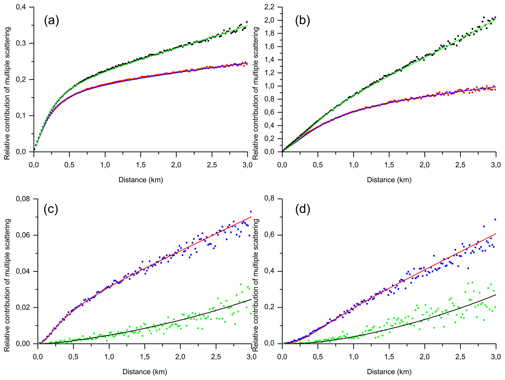
Figure A1 Monte Carlo simulations of multiple-scattering, R_MSto1 (black points); double-scattering R_2to1 (red points); and the third-order, R_3to1(d) (blue points), and fourth-order, R_4to1(d) (green points), respectively, relative contributions to lidar signals. (a, c) Water cloud. (b, d) Jet-stream cirrus. Eloranta model simulations are shown by green (MS), blue (DS), red (third-order), and black (fourth-order) curves.

Table A1 Fitting values of the EM parameters.

The results of the Monte Carlo modelling (points) and the EM's simulations (lines) are shown in Fig. A1 only for the in-cloud range of d∈[0, 3] km – i.e. the altitude interval of H∈[8, 11] km. Figure A1a and c correspond to the water cloud and Fig. A1b and d to the cirrus cloud. The microphysical and optical parameters of cloud particles are described in Sect. 2.2 above. The results of each case are divided in two; Fig. A1a and c show the relative contribution of multiple, R_MSto1(d) (black points and green line), and double, R_2to1(d) (red points and blue line), scattering; Fig. A1b and d show the relative contribution of the third, R_3to1(d) (blue points and red line), and the fourth, R_4to1(d) (green points and black line), orders. In other words, the lower panels are complementary to the corresponding upper panels. (Note that each panel in Fig. A1 has its own scale of the y axis.)

The good agreement between the MC and EM data is evident. That agreement was obtained by adjusting the EM parameters in the following way. The distance, h_b, to the cloud near edge; the extinction coefficient, ε_p(d); the half angle, ρ_t, of the receiver field of view; and the half angle, ρ_l, of the emitter divergence were assigned according to the configuration used for the MC simulations. First, we found the values of Θ_s and $P_{\mathrm{2}}\left(\mathit{\pi }\right)/P_{\mathrm{1}}\left(\mathit{\pi }\right)$ by fitting the MC data on R_2to1(d) with the Eloranta model using the ordinary least-squares approach. Then we found the values of $P_{\mathrm{3}}\left(\mathit{\pi }\right)/P_{\mathrm{1}}\left(\mathit{\pi }\right)$ and $P_{\mathrm{4}}\left(\mathit{\pi }\right)/P_{\mathrm{1}}\left(\mathit{\pi }\right)$ by fitting the MC data to R_3to1(d) and R_4to1(d), respectively. We have limited our EM simulations by five orders of scattering. Consequently, the ratio $P_{\mathrm{5}}\left(\mathit{\pi }\right)/P_{\mathrm{1}}\left(\mathit{\pi }\right)$ was computed to fit the remaining part of the total multiple scattering.

The obtained values of the parameters are shown in Table A1. The value of Θ_s is in good agreement with Eq. (A2) for the water cloud; it is about 7 % higher for the jet-stream cirrus. The important result is the fact that the values of the ratio $P_n\left(\mathit{\pi }\right)/P_{\mathrm{1}}\left(\mathit{\pi }\right),n=\mathrm{2},\mathrm{\dots },\mathrm{5}$, are quite small (especially for the water cloud) and they decrease with the order of scattering increasing. If the recommendation of the work of Eloranta (1998) – i.e. “for typical phase functions, $P_n\left(\mathit{\pi },h\right)/P_{\mathrm{1}}\left(\mathit{\pi },h\right)$ is between 0.5 and 1” – is applied, the effect of the multiple scattering will be largely overestimated in the case of the water cloud. In our opinion, the cause of the small values of the ratios $P_n\left(\mathit{\pi }\right)/P_{\mathrm{1}}\left(\mathit{\pi }\right)$ and of the declining R_MSto1(d) in the free atmosphere range is common – i.e. photons, scattered in forward and backward directions, escape the sampling volume.

We performed the same kind of work for the case of space-borne lidar and the configuration described in Sect. 4.1.1. In other words, we provide the values of parameters when the same cloud was probed by the ground-based and the space-borne lidars. The obtained values of parameters are shown in Table A1 as well. It is seen that the values of the ratio $P_n\left(\mathit{\pi }\right)/P_{\mathrm{1}}\left(\mathit{\pi }\right)$ depend not only on the phase function of particles but also on the lidar configuration – especially on the distance, the RFOV, and the EFOV.

Appendix B: An example of a simulation uncertainty analysis

It is well known that Monte Carlo modelling provides an estimate of the parameter of interest – i.e. the value that is affected by an error (an estimate minus a true value of the parameter). That error is a random variable whose mean is zero and whose width is characterized by the corresponding variance. The error is due to the statistical nature of Monte Carlo computations (see e.g. Kalos and Whitlock, 2008). In other words, a Monte Carlo estimate, like a measurement, has imperfections that give rise to random error. Such similarity provides grounds to perform a simulation uncertainty analysis using the same approach as in a measurement uncertainty analysis.

Table B1 shows the relative errors (REs) computed according to a document of the Joint Committee for Guides in Metrology (JCGM 100:2008) for our simulation data in the case of space-borne lidar (see Sect. 4.1.1 for details and the notations). The estimate of the variance was obtained using individual simulation replications (see e.g. Bicher et al., 2022). The altitudes of H=12.01 and 6.01 km correspond to the cloud-free molecular atmosphere; the altitudes of H=10.99 and 8.01 km correspond to the near edge and the far edge, respectively, of the cloud. The altitudes of 10.99, 8.01, and 6.01 km correspond to the distances of d=0.01, 2.99, and 5.99 km, respectively, in Fig. 7. The MS contribution to lidar signals and the values of R_MSto1 are close to zero at altitudes of 12.01 and 10.99 km. Therefore, the corresponding relative errors are not shown in Table B1.

Table B1 Relative error of MC simulations in percentages (%).

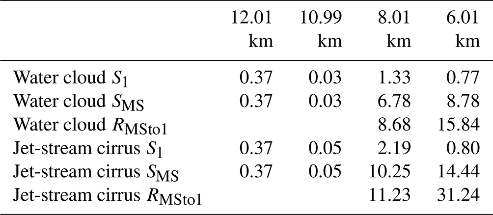
The relative errors, RE, in Table B1 can be discussed on the basis of the following relationship (Rubino and Tuffin, 2009):

$$\begin{array}{}\text{(B1)}& \mathrm{RE}\sim {\displaystyle \frac{\mathrm{1}}{\sqrt{N}\cdot \sqrt{\mathit{\chi }}}},\end{array}$$

where N is the sample size – i.e. the number of photons emitted by the lidar (2×10¹¹ and 4×10¹¹ for the water and the cirrus clouds, respectively). The variable χ is the probability of an event – i.e. the probability that an emitted photon will interact with cloud particles or the molecular atmosphere within the strobe at the altitude of interest and will be scattered towards the lidar within the RFOV. It is evident that MC modelling of lidar signals deals with rare events – i.e. the probability χ is extremely low. χ depends on particle characteristics; for example, it is inversely proportional to the lidar ratio. It is proportional to the extinction coefficient. Therefore, the REs are much better at the altitude of 10.99 km compared to 12.01 km. The probability χ is proportional to the strobe width. For example, it follows from Eq. (B1) that the relative error would be 2 times lower if the strobe were 4 times wider – i.e. the vertical resolution was 4 times worse.

To conclude this section, we underline that the quality of MC modelling can be judged by the dispersion of the data points in a figure and by values of relative errors. That is why we did not perform any smoothing of our MC data, leaving the reader to see the data quality in our figures.