Noise filtering options for conically scanning Doppler lidar measurements with low pulse accumulation

Doppler lidar (DL) applications with a focus on turbulence measurements sometimes require measurement settings with a relatively small number of accumulated pulses per ray in order to achieve high sampling rates. Low pulse accumulation comes at the cost of the quality of DL radial velocity estimates and increases the probability of outliers, also referred to as “bad” estimates or noise. Careful filtering is therefore the first important step in a data processing chain that begins with radial velocity measurements as DL output variables and ends with turbulence variables as the target variable after applying an appropriate retrieval method. It is shown that commonly applied filtering techniques have weaknesses in distinguishing between “good” and “bad” estimates with the sensitivity needed for a turbulence retrieval. For that reason, new ways of noise filtering have been explored, taking into account that the DL background noise can differ from generally assumed white noise. It is shown that the introduction of a new coordinate frame for a graphical representation of DL radial velocities from conical scans offers a different perspective on the data when compared to the well-known velocity–azimuth display (VAD) and thus opens up new possibilities for data analysis and filtering. This new way of displaying DL radial velocities builds on the use of a phase-space perspective. Following the mathematical formalism used to explain a harmonic oscillator, the VAD’s sinusoidal representation of the DL radial velocities is transformed into a circular arrangement. Using this kind of representation of DL measurements, bad estimates can be identified in two different ways: either in a direct way by singular point detection in subsets of radial velocity data grouped in circular rings or indirectly by localizing circular rings with mostly good radial velocity estimates by means of the autocorrelation function. The improved performance of the new filter techniques compared to conventional approaches is demonstrated through both a direct comparison of unfiltered with filtered datasets and a comparison of retrieved turbulence variables with independent measurements.

1 Introduction

Doppler lidars (DLs) are widely used for measurements of atmospheric wind and turbulence variables in different application areas, such as wind energy, aviation, and meteorological research (Liu et al., 2019; Sathe and Mann, 2013; Thobois et al., 2019; Krishnamurthy et al., 2013; Filioglou et al., 2022; Drew et al., 2013; O'Connor et al., 2010; Sathe and Mann, 2013; Bodini et al., 2018; Sanchez Gomez et al., 2021; Beu and Landulfo, 2022). The wide application range became possible due to the flexible configuration options of several modern systems benefitting from the all-sky-scanner technique. This technical flexibility allows for the employment of user-defined scan patterns with respect to azimuth and elevation as well as the choice of specific sampling frequencies in order to meet the data requirements for certain application-oriented retrieval processes.

At the Meteorological Observatory Lindenberg – Richard Aßmann Observatory (MOL-RAO) the interest in long-term operational DL profile observations for both wind and turbulence variables is motivated by different application aspects. The data can be helpful in analyzing and interpreting the kinematic properties of the vertical structure of the atmospheric wind and turbulence under different weather conditions and states of the ABL during the course of the day (e.g., stable ABL, convective mixed ABL, transitions between different ABL states). In addition, the profile information can be useful for regular validation purposes of atmospheric numerical models. This includes not only modeled wind profiles but also the performance of turbulence parameterizations (e.g., TKE closure) used to describe subgrid-scale processes. Due to increasingly higher model resolutions and the associated changes in the applicability and relative importance of parameterization schemes, long-term DL-based turbulence measurements are also interesting when it comes to developing appropriately adapted parameterization approaches that meet these new requirements.

A variety of scanning techniques and retrieval methods for vertical profiles of wind and turbulence variables based on DL measurements have been developed (Smalikho, 2003; Päschke et al., 2015; Sathe et al., 2015; Newsom et al., 2017; Bonin et al., 2017; Steinheuer et al., 2022). Several of these methods rely on specific scanning configurations and are tailored towards a specific data product. For the derivation of different data products this implies either the use of more than one DL system or cyclic configuration changes in a single DL. With respect to this limitation, the relatively new scanning and retrieval method introduced by Smalikho and Banakh (2017) stands out from other methods. Their approach is based on a carefully derived set of model equations, describing functional relationships between radial velocity observations measured along a conical scan with high azimuthal and temporal resolution (Δθ∼1°, Δt∼0.2 s) and a set of meaningful wind turbulence variables such as turbulence kinetic energy (TKE), eddy dissipation rate (EDR), momentum fluxes, and the integral scale of turbulence. Hence, the essential benefit of this approach relies on the deployment of an internally consistent set of simultaneous wind and turbulence profile observations based on just one scan strategy. As a further outstanding feature the method provides correction terms to account for the typical underestimation of the TKE due to the averaging over the pulse volume of the DL. This issue has frequently been mentioned as the most challenging task in turbulence measurements using DL (Sathe and Mann, 2013; Liu et al., 2019).

Because of the strength of the Smalikho and Banakh (2017) approach, the method has been implemented and tested for routine application at MOL-RAO. From the first quasi-routine test measurements with a StreamLine DL from the manufacturer HALO Photonics (now HALO Photonics by Lumibird) three things became apparent: (1) the measurements of radial velocity show an increased level of noise which is noticeable through an increased number of outliers (“bad” estimates) even at rather low height levels in the ABL; (2) the reliability of both retrieved wind and above all turbulence variables strongly depends on the degree of noise contamination, i.e., the number and distribution of bad radial velocity estimates, in the input data; and (3) if just the signal-to-noise ratio (SNR) thresholding technique is used to remove noise from the data, the final turbulence product availability is relatively low. The first finding can be attributed to short accumulation times, which is an inevitable consequence of the technical realization of the scanning strategy with high spatiotemporal resolution. The length of the accumulation time determines how many available spectra of backscattered light can be used to estimate the frequency shift f_d (Doppler frequency) and therewith the radial velocity defined through $V_{\mathrm{r}}=-\mathit{\lambda }{f}_{\mathrm{d}}/\mathrm{2}$. The longer a signal is sampled, the more accurate this estimation will be. For that reason it is a common approach to accumulate the spectra of backscattered light from multiple pulses N_a (Frehlich, 1995; Rye and Hardesty, 1993; Banakh and Werner, 2005; Li et al., 2012). For the retrieval of wind profiles as proposed in Päschke et al. (2015), for instance, DL measurements have been performed using a comparably high number of N_a = 75 000 pulses. At this point the method of Smalikho and Banakh (2017) requires a sensible compromise. Using a StreamLine DL, for technical reasons a conical scan with the required high azimuthal and temporal resolution can only be achieved with a rather low number of accumulated pulses per measurement ray, i.e., N_a∼2000. This in turn has the consequence that the occurrence of bad estimates in the measurements becomes more likely (Frehlich, 1995). Such outliers contain no wind information (Stephan et al., 2018), and, if not excluded from the measured dataset, they may contribute to large errors in the retrieved meteorological variables (Dabas, 1999). The latter explains the aforementioned second finding and indirectly confirms the recommendations given in Banakh et al. (2021) that the method for determining wind turbulence parameters presented in Smalikho and Banakh (2017) is only applicable if the probability P_b of bad estimates of the radial velocity is close to zero. A closer examination of the third finding mentioned above revealed that with the proper choice of the threshold value the SNR thresholding technique is indeed very effective in removing noisy data, but it also bears the risk of discarding a lot of reliable measurements. This in turn proves to be ineffective for the overall product availability and would not justify a routine application of the retrieval method.

To overcome the issues described above, new filter methods were developed in the course of implementing the retrieval method by Smalikho and Banakh (2017) for routine applications at MOL-RAO. In particular, a filter method was sought which allows for a reliable removal of all noise contributions and circumvents an unnecessary refusal of reliable data at the same time. A detailed presentation of these methods is the main objective of this work. In addition, their advantages over commonly used filtering techniques for turbulence-measurement-oriented routine applications are presented. The article is organized as follows: in Sect. 2 technical information on the measuring system used, its configuration, and typical characteristics in measured data due to short accumulation times is given. To motivate the need for new ideas of improved filtering techniques, pros and cons of common filter methods to detect bad estimates are discussed in Sect. 3. In Sect. 4 a new type of visualization for analyzing DL measurements from conical scans is presented. Building on this, ideas for two new filter approaches are developed and discussed. An overview of how the new filter methods affect the quality of retrieved turbulence variables using the method by Smalikho and Banakh (2017) is provided in Sect. 5.

2 Doppler lidar measurements

The DL measurements serving as the basis for this work were taken at the boundary-layer field site Falkenberg (in German: Grenzschichtmessfeld, GM, Falkenberg), which is an open field embedded in a flat landscape, with main wind directions from WSW, located about 5 km to the south of the MOL-RAO observatory site. The flat terrain characteristics meet the requirements for the application of the turbulence measurement approach by Smalikho and Banakh (2017) in non-complex terrain.

2.1 Technical system specifications and configuration

At GM Falkenberg a StreamLine DL from the manufacturer HALO Photonics with the specifications given in Table 1 was used and operated using a conical-scan-mode configuration to apply the turbulence retrieval approach by Smalikho and Banakh (2017). This configuration is defined by three key parameters, namely the elevation angle (ϕ=35.3°), the azimuthal resolution (Δθ∼1°), and the time duration for one single scan (T_scan=72 s). In order to realize this scanning strategy the DL was configured to be in continuous scan motion (CSM) while sampling data. A custom scan file (see Appendix A) has been defined for the scanner configuration including information about the angular rotation rate ω_s, the start and end positions of the scanner, and the elevation angle ϕ. In analogy to the work of Smalikho and Banakh (2017) we set ω_s=5° s⁻¹ to nearly satisfy Δθ∼1°. Note that the latter implies measurements on an irregular grid which for analysis purposes later on requires the transfer of the data to an equidistant grid with Δθ=1°. The specific value for ϕ goes back to an earlier theoretical work of Kropfli (1986) and Eberhard et al. (1989), who focused on Doppler-radar-based turbulence measurements. In addition, Teschke and Lehmann (2017) have shown that using DL this value is also an optimum beam elevation angle for a mean wind retrieval with a minimum in the retrieval error. With the specifications for Δθ and ω_s and due to the pulse repetition frequency f_p=10 kHz (see Table 1) we had to adjust the configuration setting for the number of pulses per ray to N_a=2000 using the relation $N_{\mathrm{a}}=\mathrm{\Delta }\mathit{\theta }{f}_{\mathrm{p}}/{\mathit{\omega }}_{\mathrm{s}}$ (Banakh and Smalikho, 2013). This is a minor difference compared to the value suggested in Smalikho and Banakh (2017), i.e., N_a=3000, which is due to a higher pulse repetition frequency, i.e., f_p=15 kHz, characterizing their DL system. Note that for StreamLine DL systems the system-specific parameter f_p cannot be changed by the user. The low value for N_a is non-favorable if a high measurement quality is needed. For best possible measurement quality in the lower ABL it is therefore important to use the focus setting option to improve the signal intensities within a selected height range. For the DL used in our studies (DL78 hereafter) the focus was set to 500 m. Working with StreamLine DL systems, the range resolution ΔR along the line of sight (LOS) can also be adjusted. For reasons of compatibility with the pulse length of τ_p=180 ns the range resolution was set to $\mathrm{\Delta }R=c{\mathit{\tau }}_{\mathrm{p}}/\mathrm{2}\approx \mathrm{30}$ m, where c denotes the speed of light.

Table 1 Instrument specifications of the HALO Photonics StreamLine DL operated at MOL-RAO.

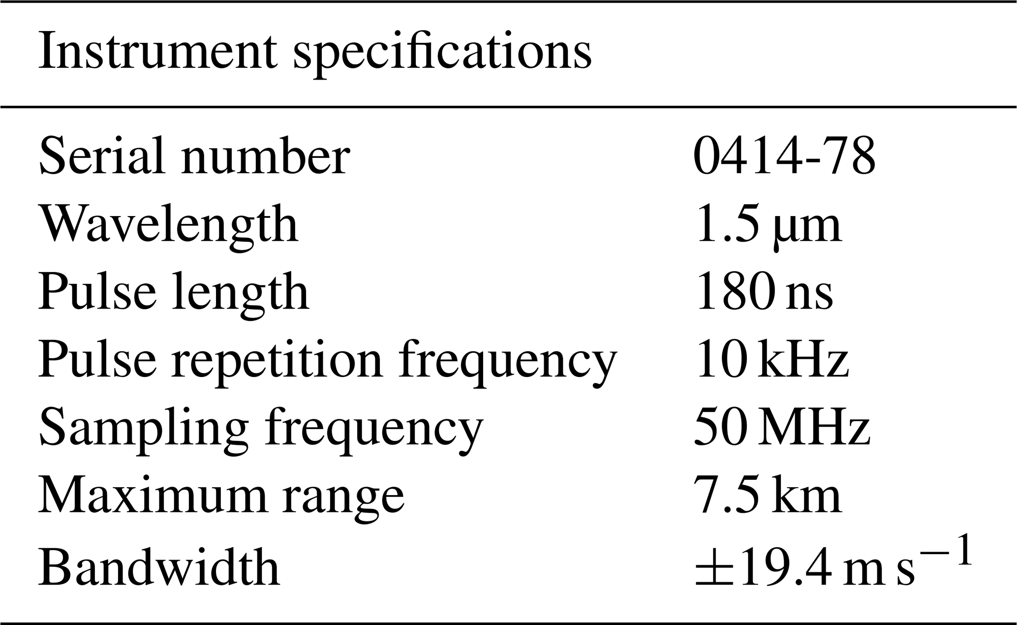
Note that with StreamLine XR DL systems HALO Photonics by Lumibird offers a further development of the StreamLine series. XR systems operate with larger pulse length in order to increase the range, depending on the presence of scattering particles in the atmosphere. The larger pulse length, however, reduces the spatial resolution of the measurements along the line of sight (LOS), which is not an option for measurements in the ABL if the focus is on the detection and investigation of small-scale structures.

2.2 Typical measurement examples and their noise characteristics

For the measurements carried out in this work the relevant DL output variables are the radial velocity estimates V_r along each single LOS of the conical scan and the associated SNR values. The estimation of V_r is based on the determination of the Doppler shift f_d of the backscattered signal by an onboard signal processor. A number of methods are available to determine f_d (Frehlich, 1995), but the DL manufacturers usually do not disclose to the customer the details of the implemented algorithm. The performance of the estimation algorithms and thus the quality of V_r may vary. The assessment of the performance of the estimation algorithms is generally based on the probability density function (PDF) of the velocity estimates. According to Frehlich (1995), the PDF of velocity estimators performing well is characterized by a localized distribution of “good” estimates centered around the true mean velocity and a fraction of uniformly distributed bad estimates. This leads to the following frequent distinction in DL radial wind measurements:

$$\begin{array}{}\text{(1)}& V_{\mathrm{r}}=\left\{\begin{array}{ll}{V}_{\mathrm{r}}+V_{\mathrm{e}}& \text{in the case of good estimate}\\ V_{\mathrm{b}}& \text{in the case of bad estimate},\end{array}\right.\end{array}$$

with V_e denoting a random instrumental error (Stephan et al., 2018). In the literature, bad estimates are mostly described as random outliers or noise uniformly distributed over the resolved velocity space (Frehlich, 1995; Dabas, 1999). It can be shown that the occurrence of noise in a series of radial velocity measurements based on a conical scan can be determined by means of the autocorrelation function (ACF) evaluated at lag 1 (Appendix B). In particular, for a conical scan with high azimuthal resolution of Δθ∼1° as used in this work, ACF = 1 indicates noise-free measurements, while ACF < 1 gives an indication of the occurrence of noise.

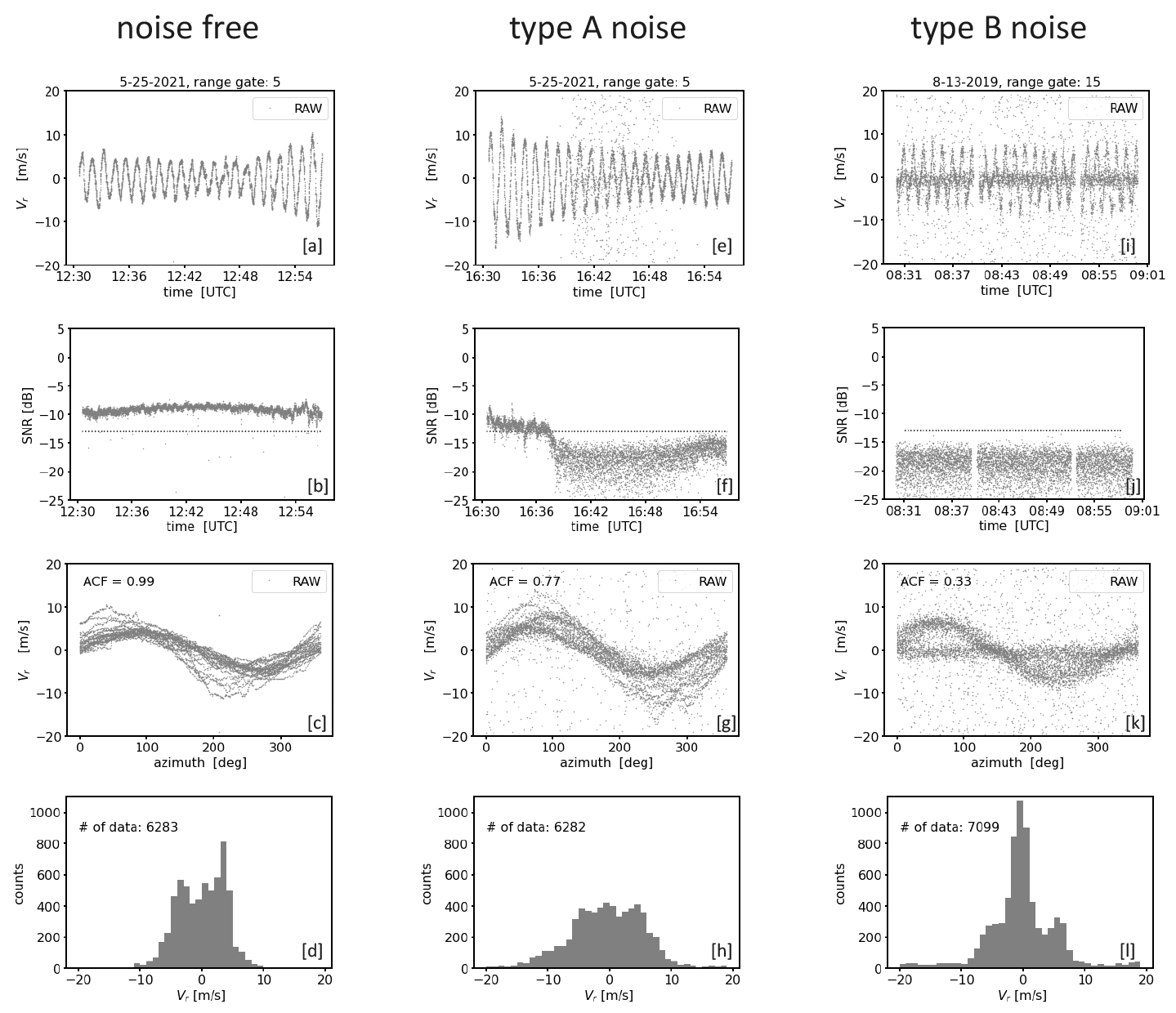
Figure 1 Examples for measurements from one and the same conically scanning Doppler lidar. Each column represents measurements during a 30 min interval at different times and range gates (i.e., measurement heights along the line of sight) which are characterized by different kinds of noise (left: noise-free, middle: type A noise, right: type B noise). The plots of each row depict the measurements from different perspectives. The first row shows a time series plot of the radial velocities (V_r) (a, e, i). In a similar way the second row (b, f, j) illustrates the corresponding signal intensities (SNR) of the measurements. Here, the horizontal dotted line indicates an SNR threshold level calculated as proposed in Abdelazim et al. (2016) for N_a=2000 (see Sect. 3.1). The third row (c, g, k) shows the DL measurements from a VAD perspective, i.e., a display of the radial velocity as a function of the azimuth angle. The ACF value indicates the degree of noise contamination in the measured time series (see Appendix B). The fourth row (d, h, l) shows histograms of V_r.

Typical examples for DL78 measurements that differ in terms of their noise characteristics are shown in Fig. 1. Each measurement example reflects a different 30 min time period and range gate height. Per column, different analysis diagrams are provided for each measurement example. Noise-free measurements indicated by ACF = 1 (Fig. 1c) are shown in the column on the left. Apart from the superimposed small-scale fluctuations which reflect natural turbulent fluctuations, the time series plot of radial velocities (Fig. 1a) and the corresponding velocity–azimuth display (VAD) plot (Fig. 1c) show a clean sinusoidal course without any random outlier. The sinusoidal course is typical for measurements with conically scanning DL systems and manifests itself in a U-shaped bimodal distribution of the radial velocities provided the wind field was stationary (Fig. 1d). In the middle and right columns the measurements are contaminated with noise, which is indicated by ACF = 0.8 and ACF = 0.3, respectively (Fig. 1g, k). Here, the periodic signals are temporarily interrupted by bad estimates randomly representing “any” value in the velocity range ±19 m s⁻¹ (Fig. 1e, i). Furthermore, differences in the distribution of bad estimates are noticeable. In contrast to the measurements in the middle column where the bad estimates appear quite uniformly distributed (type A noise hereafter), an additional higher aggregation of bad estimates around zero (type B noise hereafter) is noticeable in the right column. This becomes particularly clear by comparing the corresponding panels with the VAD diagrams (Fig. 1g, k) and those with the histograms of the radial velocities (Fig. 1h, l). Note that contrary to Fig. 1d the characteristic U-shaped distribution in Fig. 1l can no longer be recognized because it mixes with a Gaussian-like distribution of bad estimates. Finally, for each measurement example a clear difference in the level of the signal intensities is noticeable (Fig. 1b, f, j). With SNR values around −10 dB the signals are strong in the noise-free case, and with values smaller than −15 dB the signals are weak in the noisy cases. It is important to point out that for the noisy cases the signal levels are mostly the same and thus do not provide any indication about the type of noise distribution.

All three measurement examples have been taken with the same DL system under identical configuration (e.g., N_a = 2000 pulse accumulations). Despite the low pulse accumulations there are measurement cases with and without noise. This can be explained by the natural variability in the atmospheric aerosol content over the course of a day and with altitude. Aerosols act as backscattering targets and their atmospheric loading influences the quality of the DL signals and therewith the amount of noise in the measurements. A sufficiently large amount of aerosol can contribute to noise-free DL measurements even for low pulse accumulations. Little aerosol combined with low pulse accumulation, however, represents an unfavorable constellation for achieving good data quality.

Concerning the differences in the bad estimate distributions, to the authors' knowledge up to now there have been no user reports about nonuniform bad estimate distributions in DL measurements available. A uniform distribution of bad estimates indicates that the noise component of the spectrum of the lidar signal is white noise (Stephan et al., 2018). It is believed that additional non-white DL noise sources such as shot noise, detector noise, relative intensity noise (RIN), and speckles (Hellhammer, 2018) cause these nonuniform type B noise characteristics. At this point more in-depth investigations would be necessary but cannot be carried out within the scope of this work. It is worth pointing out, however, that the occurrence of type B noise is not a system-specific DL78 problem. During the () (Field Experiment on Sub-mesoscale Spatio-Temporal Variability in Lindenberg) campaign (Hohenegger et al., 2023), there was the opportunity to compare the measured data from three StreamLine and four StreamLine XR Doppler lidars (see Sect. 2.1) positioned side by side and configured identically using the scan mode outlined in Smalikho and Banakh (2017). The comparison revealed type-B-like noise contamination within the measured data for several systems albeit to varying degrees (see Figs. C1 and C2 in Appendix C). This suggests that this type B noise issue is at least typical for StreamLine DL systems.

3 Pros and cons of commonly used filtering techniques

In the previous section it has been shown that DL radial velocity measurements obtained using the measurement strategy proposed in Smalikho and Banakh (2017) can show a strikingly high proportion of noise. The successful application of the associated retrieval method to determine turbulence variables from DL measurements, however, requires a probability of bad estimates close to zero (Smalikho and Banakh, 2017; Banakh et al., 2021). Hence, a careful pre-processing of measurement data to detect and remove noise is necessary.

Different filtering techniques to separate reliable data from noisy measurements can be found in the literature. A closer look at the underlying principles of radial velocity quality assessment allows a rough subdivision into two categories of filtering methods: (1) one category makes use of additional parameters from post-processing of Doppler spectra and (2) the other uses statistical analysis tools applied to time series of DL radial velocity estimates. The method behind the first category is the well-known SNR thresholding technique. Methods representing the second category are, for instance, the median absolute deviation (MAD) originating from Gauss (1816), consensus averaging (CNS) introduced by Strauch et al. (1984), the filtered sine wave fit (FSWF) by Smalikho (2003), or the integrated iterative filter approach by Steinheuer et al. (2022). The last two methods mentioned are directly integrated into a retrieval method for wind or wind gusts. A more detailed review of these and further filtering methods that belong to the second category mentioned above is given in Beck and Kühn (2017). In this section the advantages and disadvantages of these different filtering method categories are examined using the SNR and CNS filter as an example.

3.1 SNR thresholding

The signal-to-noise ratio (SNR) is determined from the Doppler spectra and is defined as the ratio between the signal power and the noise power. The first bears the meaningful information in a measurement and the latter is considered to be an unwanted signal contribution that is blurring this information. The higher the level of signal power and the smaller the level of noise power, the better the SNR and thus the quality of the radial velocity estimate.

In practice, DL users are often faced with deciding on a suitable SNR threshold value (SNR_thresh hereafter) to separate good from bad estimates. Depending on how the measurement data are used later on, the expected uncertainty of the radial wind velocity also plays a role in this decision. Pearson et al. (2009) provide a guideline on that issue based on an experimental approach. The results showed good agreement with theoretical results based on an approximate equation introduced by Rye and Hardesty (1993), reading

$$\begin{array}{}\text{(2)}& \mathit{\sigma }=\mathrm{2}{\left({\mathit{\pi }}^{\mathrm{0.5}}/\mathit{\alpha }\right)}^{\mathrm{0.5}}(\mathrm{1}+\mathrm{0.16}\mathit{\alpha })\left(\mathrm{\Delta }\mathit{\nu }/N_{\mathrm{p}}^{\mathrm{0.5}}\right),\end{array}$$

with $\mathit{\alpha }=\mathrm{SNR}/\left(\right(\mathrm{2}\mathit{\pi }{)}^{\mathrm{0.5}}(\mathrm{\Delta }\mathit{\nu }/B))$ and N_p=M N_a (SNR). Here, σ denotes the error estimate of the radial velocity in the weak signal, multipulse-averaged regime, N_a the number of accumulated pulses, B the bandwidth, Δν the signal spectral width, and M the gate length in points. For more details see Appendix D. Note that Eq. (2) can be used in two ways. On the one hand, it provides an estimate for the uncertainty of the radial velocity estimate depending on the SNR. On the other hand, it provides guidance to calculate SNR_thresh for a prescribed acceptable uncertainty in the Doppler lidar estimate. Examples for an evaluation of Eq. (2) for different numbers of N_a are given in Fig. 2. The curves basically show how the uncertainty of the measurements decreases with increasing SNR. Additionally, the effect of pulse accumulation becomes visible. For the same requirement on the uncertainty of the Doppler estimate, e.g., σ<0.5 m s⁻¹ or σ< 0.1 m s⁻¹, the corresponding SNR threshold value for reliable data would be lower for Doppler estimates based on higher pulse accumulations (e.g., SNR_thresh = −24 dB or SNR_thresh = −17 dB for N_a = 30 000) than for Doppler estimates based on a lower number of pulse accumulations (e.g., SNR_thresh = −18.5 dB or SNR_thresh = −11 dB for N_a=2000). Another approximate equation to determine SNR_thresh is suggested in Abdelazim et al. (2016). Taking into account the number of accumulated pulses N_a only, they propose the following equation for an SNR threshold determination:

$$\begin{array}{}\text{(3)}& {\mathrm{SNR}}_{\mathrm{thresh}}={\displaystyle \frac{\mathrm{1}}{\sqrt{N_{\mathrm{a}}}}}+{\displaystyle \frac{\sqrt{\mathrm{2}}}{\sqrt{N_{\mathrm{a}}}}}.\end{array}$$

Example results for SNR_thresh derived from Eq. (3) for different N_a are also given in Fig. 2.

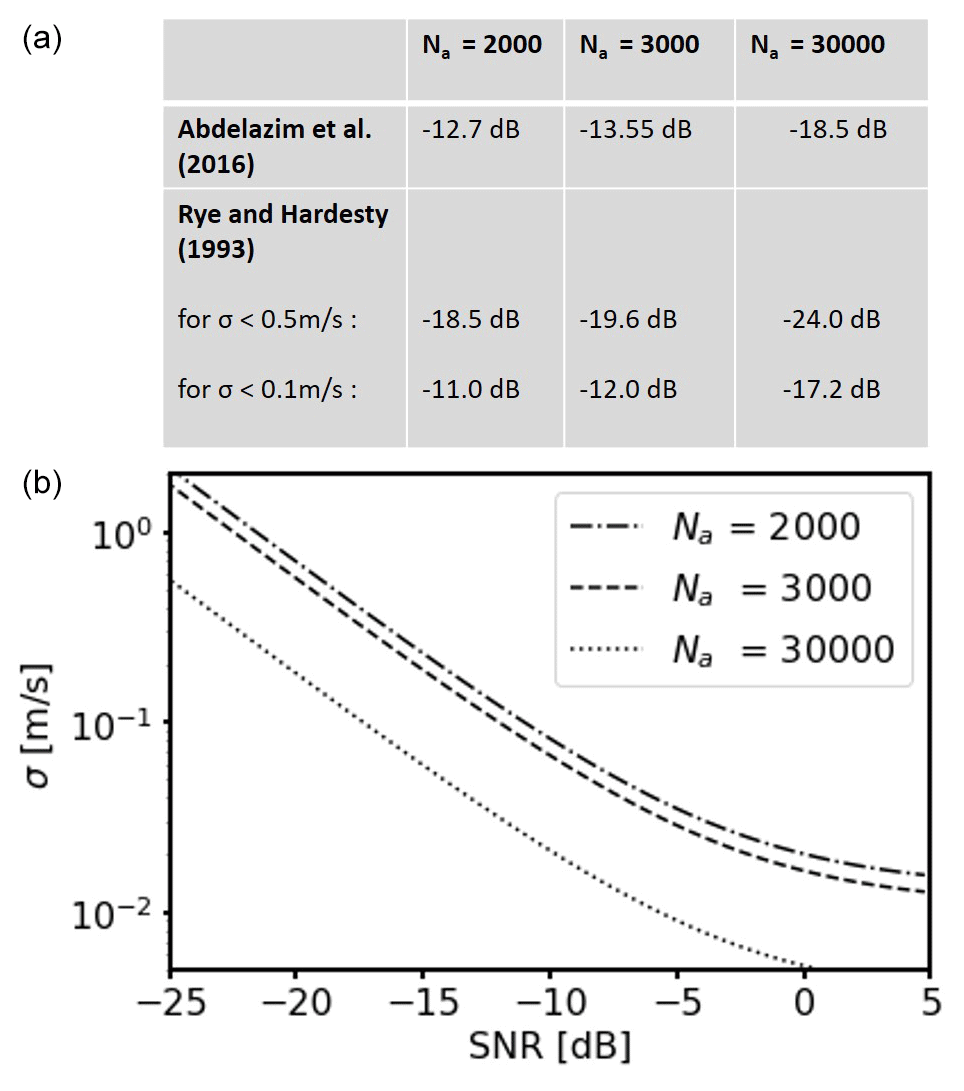
Figure 2 (a) Examples of calculated SNR threshold values depending on the number of accumulated pulses N_a based on the approach by Abdelazim et al. (2016) and the approach by Rye and Hardesty (1993). (b) Example plots for the change in the theoretical standard deviation σ of the Doppler velocity estimates depending on the signal-to-noise ratio (SNR) following the approach by Rye and Hardesty (1993). The curves are valid for different N_a and the following system-specific parameters: B=2 × 19 m s⁻¹, M=10, Δν=1.3 m s⁻¹.

The turbulence retrieval proposed by Smalikho and Banakh (2017) requires measurements with a probability of bad estimates close to zero. The example shown in Fig. 3 clearly illustrates that with SNR_thresh = −12.7 dB calculated by means of Eq. (3), a universally valid first-guess SNR threshold satisfying this requirement across all measuring height ranges can be obtained. Here, estimates for V_r from range gate number 4 to 99 are displayed against their associated SNR values. While bad estimates randomly filling the entire search band ±19 m s⁻¹ can be observed to the left of the threshold line, none can be found to the right. If one further relaxed this threshold, the probability of bad estimates would increase. From Eq. (2) it can be additionally inferred that with SNR_thresh = −12.7 dB measurement uncertainties less than 0.1 m s⁻¹ can be expected. Though it is important to note that by applying $SN{R}_{\mathrm{thresh}}=-\mathrm{12.7}$ dB to DL radial velocity measurements, as shown with the examples given in Fig. 1 as well as Fig. 5a, c, and e, a huge fraction of obviously good estimates would be discarded. A reduction of data availability would be the consequence, making a representative derivation of wind and turbulence products often difficult or even impossible. This is a limiting factor of this kind of approach to distinguish between good and bad estimates (Dabas, 1999).

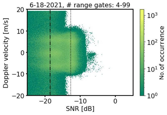
Figure 3 Doppler velocity vs. SNR plot from conically scanning Doppler lidar measurements with N_a = 2000 accumulated pulses. The plot includes full-day measurements for all range gates between the 4th and 99th range gate. The vertical lines denote different SNR thresholds based on different approaches, namely by Abdelazim et al. (2016) with a Doppler velocity uncertainty of σ<0.1 m s⁻¹ (dot) and by Rye and Hardesty (1993) with a Doppler velocity uncertainty of σ<0.5 m s⁻¹ (dash–dot). See Fig. 2 for exact SNR threshold numbers.

3.2 Consensus averaging

Methodically different from the SNR thresholding technique is the consensus averaging (CNS) method introduced by Strauch et al. (1984). The method was originally developed to exclude outliers from radar wind profiler data. A schematic that explains the CNS approach is shown in Fig. 4. Here noise-contaminated measurements of V_r from several single conical scans executed one after the other are displayed using the VAD perspective. Separating the range of measurement directions (0 to 360°) into equidistant intervals $I_i=\left[\right(i-\mathrm{1})\mathrm{\Delta }\mathit{\theta },i\mathrm{\Delta }\mathit{\theta }]$ ($i=\mathrm{1},\mathrm{2},\mathrm{3},\mathrm{\dots },n$ with n∈ℕ), the basic idea is to seek within each I_i along the V_r axis for this subset of data satisfying both (i) the occurrence within a prescribed interval ΔV_r, which is assumed to be a typical value for the atmospheric wind variance, and (ii) the provision of data availability $X_i^{max}$ which, however, must not fall below a prescribed value X_thresh. Similar to the SNR thresholding technique, the difficulty exists in a meaningful choice of ΔV_r and X_thresh as will be shown in more detail below.

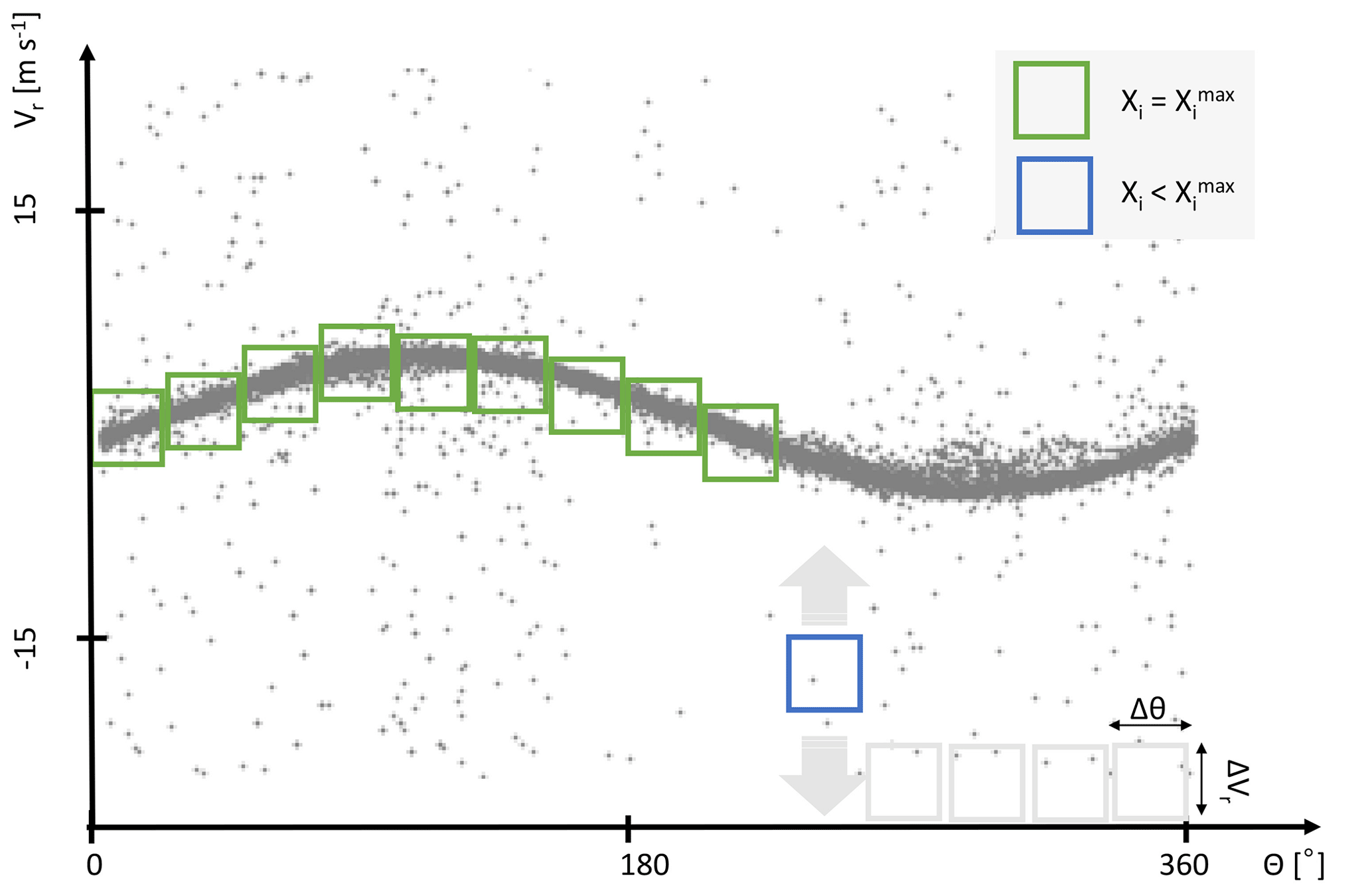
Figure 4 Schematic representation of a possible practical implementation of the CNS (consensus) averaging method based on an approach by Strauch et al. (1984) (see Sect. 3.2). The data in the green boxes have already been identified as reliable. The blue box illustrates the process of searching the reliable data, and the gray boxes stand for azimuthal intervals that still need to be analyzed.

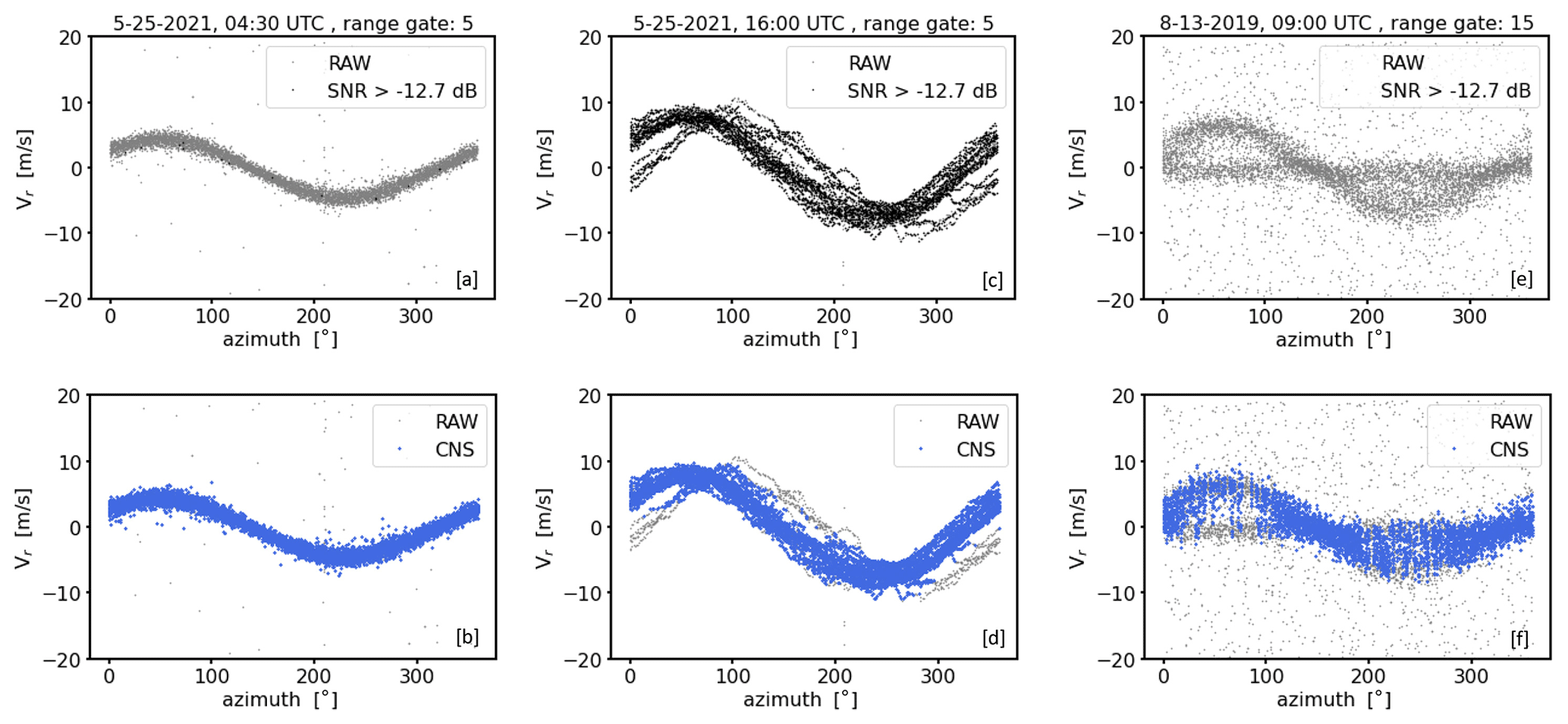
Figure 5 VAD plot examples from conical DL measurements with N_a = 2000 pulse accumulations illustrating the application of the SNR thresholding (a, c, e) and the CNS (b, d, f) noise filtering method. The examples represent three different 30 min measuring intervals at different range gates and with different levels of noise contamination. The SNR threshold value of −12.7 dB has been calculated using the approach by Abdelazim et al. (2016). Δθ=1° and ΔV_r = 3 m s⁻¹ were used for the application of the CNS.

If the focus is on the derivation of turbulence variables, including the determination of variances caused by eddies in turbulent flow, the problem of this CNS approach is that it requires an a priori estimate of the variance which is actually being attempted to be derived. If ΔV_r does not correspond to the true atmospheric situation, e.g., the assumed value for ΔV_r is too small or too large, it may happen that either measurements bearing relevant wind information are rejected or that bad estimates remain in the dataset. Examples of this are given in Fig. 5b, d, and f assuming ΔV_r=3 m s⁻¹ and X_thresh=60 %. The early morning 30 min measurement example from 25 May 2021 with the timestamp 04:30 UTC (Fig. 5b) shows noise-contaminated DL measurements during weak wind and turbulence conditions. At this time the actual wind variance was obviously lower than assumed by ΔV_r so that the prescribed interval ΔV_r gave room for the inclusion of bad estimates which had to be accepted as reliable due to the CNS concept. The afternoon example from 25 May 2021 with the timestamp 16:00 UTC (Fig. 5d) shows DL measurements during stronger wind and turbulence conditions than in the morning. Additionally, at some point during the 30 min interval a change in the wind direction contributes to a phase shift in the sine signal represented by some of the scan circles. Mainly because of this nonstationarity the variability of the Doppler velocity measurements is obviously larger than assumed by ΔV_r=3 m s⁻¹ in some azimuth sectors so that relevant information characterizing this nonstationarity remains outside of the interval ΔV_r and is discarded by the CNS. Note that at this point the focus is on the performance of the CNS and not on reconstructed wind and turbulence variables. Hence, this non-applicability of the CNS method during nonstationary measuring intervals needs to be considered apart from the question of whether a derivation of wind and turbulence variables is meaningful if nonstationarity occurs. In Sect. 5 it will be shown that a wrong inclusion of bad estimates or a false exclusion of good estimates because of a non-compatible ΔV_r compared to the actual atmospheric situation has the consequence that turbulence products (e.g., TKE) calculated based on improperly pre-filtered measurement data may be either overestimated or underestimated.

Another limitation of the CNS filtering technique is that it expects a uniform distribution of bad estimates for a successful application. This becomes evident by considering the CNS filtering results for the measurement example shown in Fig. 5f. This example represents the type B noise case shown in Fig. 1. Here, the subsets of Doppler velocities found by the CNS for some of the azimuthal sectors often do not represent the desired good estimates because the high density of bad estimates around zero erroneously shifts the range ΔV_r bearing a maximum of data availability towards zero. In this case the nonuniform distribution of the bad estimates makes a successful application of the CNS impossible. Note that the disadvantages worked out here can be generalized to all statistical methods used for outlier detection which require additional assumptions about the distribution and the variance of the quantity of interest.

4 Ideas for new filtering techniques

The filtering techniques discussed in the previous section are not efficient enough if DL measurements with both the highest possible data availability and a probability of bad estimates close to zero are required. New filtering techniques with improved performance concerning this demand are presented in this section. In particular, depending on the measurement's noise characteristics two different approaches (referred to as approach I and approach II hereafter) for new filter techniques are discussed. Including a coarse filter and a filter for post-processing each approach consists of two separate filtering steps which are carried out one after the other, i.e., approach I = coarse filter I + filter for post-processing and approach II = coarse filter II + filter for post-processing, while using different perspectives of data representation to analyze the occurrence of bad estimates in the DL measurements. Both coarse filters make use of the VV90D perspective, which will be introduced in Sect. 4.1. The application of the post-processing filter requires the well-known VAD perspective.

4.1 Framework of the VV90D perspective

The VV90D perspective represents a diagram in a rectangular coordinate system where each radial velocity value V_r obtained from a conically scanning DL is plotted versus its counterpart measured at an azimuthal shift of 90°. In particular, for a time series of radial velocity measurements $V_{\mathrm{r}}(R,\mathit{\theta };t)$ this means that $V=V_{\mathrm{r}}(R,\mathit{\theta };t)$ is plotted along the y axis and $V\mathrm{90}=V_{\mathrm{r}}(R,\mathit{\theta }-\mathrm{90}\mathit{°};t^{\ast })$ is plotted along the x axis. Here, R denotes the range gate, θ the azimuth angle along the scan circle, and t the timestamp of the measurement. Note that t^∗ denotes the timestamp of the shifted counterpart value. The motivation underlying this graphic representation of DL measurements will be explained in more detail using the two noise-free measurement examples shown in Fig. 6. In particular, measurements from a conically scanning DL visualized in both a V_r−t diagram and a VV90D plot are shown in Fig. 6a and d and Fig. 6b and e, respectively. The plots in the upper line reflect a homogeneous and stationary measurement example (case 1) which can be clearly seen by the smooth sinusoidal course of the radial velocity, i.e., V∼sin (θ), with a nearly constant amplitude (Fig. 6a). The same measurement example visualized in a VV90D diagram shows clear circular patterns (Fig. 6b). The latter can be explained by taking the phase shift identity $\sin (\mathit{\theta }-\mathrm{90}\mathit{°})=-\cos \mathit{\theta }$ into account, yielding $V\mathrm{90}\sim -\cos \mathit{\theta }$. Therewith paired data points ($x=V\mathrm{90},y=V$) plotted in a rectangular coordinate system describe a circle. Note that this way of looking at DL measurements shows analogies to the harmonic oscillator where the time evolution of both displacement and motion are frequently visualized in a phase-diagram plot to show the 90° phase relationship between velocity and position much more clearly (Vogel, 1997). The plots in the lower line of Fig. 6 represent a nonstationary measurement example (case 2). Due to the sinusoidal course superimposed with smaller fluctuations and a varying amplitude (Fig. 6d) the corresponding VV90D diagram (Fig. 6e) of the same measurements shows a slightly wider and more blurred ring structure.

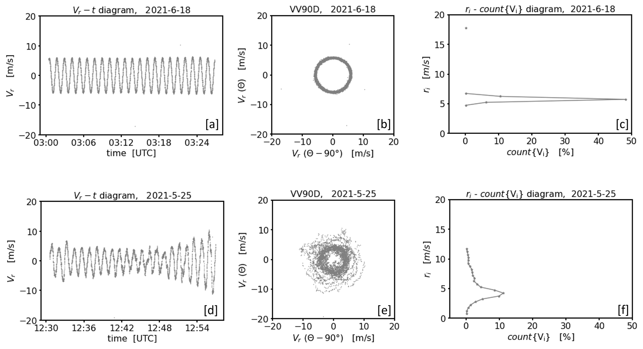
Figure 6 Examples of a graphical visualization of radial velocity measurements from a conically scanning DL using the framework of the VV90D perspective for two cases with stationary (a–c) and nonstationary (d–f) winds. The panels in each row illustrate in sequence: a time series plot of the measured radial velocity over a 30 min time period (a, d), the same data plotted using the VV90D perspective (b, e), and the frequency distribution of data points in the VV90 plane binned by circular rings $r_i-\mathrm{\Delta }r\le r_i\le r_i+\mathrm{\Delta }r$, where $i=\mathrm{1},\mathrm{\dots },n$ (n∈ℕ) and Δr=0.5 m s⁻¹ (c, f).

A quantitative description of the VV90D ring structures is provided with the diagrams shown in Fig. 6c and f. These diagrams are referred to as r_i−count{V_i} diagrams hereafter. Here, r_i denotes the radius of a pre-defined circular ring $r_i-\mathrm{\Delta }r\le r_i\le r_i+\mathrm{\Delta }r$ with origin at ($x=\mathrm{0},y=\mathrm{0}$) and width Δr in the VV90 plane. The quantity count{V_i} denotes the number of measurement data that can be found in this ring. Note that these data represent a circular-ring-related subset V_i of the whole measurement series, i.e., V_i⊂{V}. Taking the equation of a circle into account, i.e., $r=x^{\mathrm{2}}+y^{\mathrm{2}}$, in practice both the subset V_i and count{V_i} can be determined by identifying the radial velocities $V=V_{\mathrm{r}}(R,\mathit{\theta };t)$ of the measurement time series that satisfy the relation

$$\begin{array}{}\text{(4)}& r=\sqrt{V{\mathrm{90}}^{\mathrm{2}}+V^{\mathrm{2}}},\end{array}$$

with the range of radii r defined through the boundaries of the circular ring $r_i-\mathrm{\Delta }r\le r_i\le r_i+\mathrm{\Delta }r$. In order to generate the r_i−count{V_i} diagrams shown in Fig. 6c and f the full area of the VV90 plane has been subdivided into closely spaced circular rings of increasing radius ($i=\mathrm{0},\mathrm{\dots },n$ with n∈ℕ) with discrete fixed steps Δr=0.5 m s⁻¹. Note that this value turned out to be a viable choice if using the r_i−count{V_i} diagram as a tool in a filtering procedure (see Sect. 4.2). For case 1, the data availability of measured radial velocities is constrained to only a few circular rings with r_i ranging between 5 and 6.5 m s⁻¹, with the largest fraction of measurements in the circular ring with r_i = 5.5 m s⁻¹ (see Fig. 6c). Additionally, due to the stationary wind field conditions the obtained availability distribution is strictly unimodal and symmetric. For case 2 the measurements are distributed over a broader range of circular rings with r_i taking values between 0.5 and 12.5 m s⁻¹. The largest fraction of the measurements occurs within a circular ring with r_i = 4.5 m s⁻¹ (see Fig. 6f). The distribution of data availability is nearly unimodal but asymmetric. The examples shown in Fig. 6 represent just two specific situations, and a great variety of VV90D and associated r_i−count{V_i} diagrams may result for different atmospheric and lidar signal conditions, including multi-modal distributions (not shown here). In the following we refer to the VV90D diagram and the associated r_i−count{V_i} diagram as the framework of the VV90D perspective.

Compared to the commonly used VAD visualization technique, the framework of the VV90D perspective represents an alternative way of displaying radial velocity measurements from a conically scanning DL and opens up new possibilities for data analysis at the same time. In the next section it will be shown how this framework can be used to develop suitable filtering techniques of bad estimates in noisy DL data.

4.2 Coarse filtering techniques

Two different coarse filtering techniques are presented next. The underlying ideas are motivated by characteristic features of good and bad estimates in the VV90D diagram, which will be briefly explained. For this purpose the noise-contaminated measurement examples of type A and type B from Sect. 2.2 are used. Compared to noise-free DL measurements, noticeable features of noise-contaminated DL measurements in the VV90D are the greater spread of paired DL data ($x=V\mathrm{90},y=V$) and a lack of clear circular patterns (Fig. 7a, d). In the associated r_i−count{V_i} diagrams (Fig. 7b, e) this also goes along with a broader distribution of available data points over a larger range of circular rings. Furthermore it is obvious that for the type B noise measurement example the more densely distributed bad estimates around zero make a cross-shaped region visible in the VV90D (Fig. 7d) and cause a pronounced secondary peak in the r_i−count{V_i} diagram (Fig. 7e). Additionally, by examining in more detail the properties of the data occurring in the three color-coded circular rings, it becomes apparent that circular rings with a high data number mostly contain reliable DL radial velocities, i.e., good estimates. This can be seen from the fact that the data occurring in these rings mostly follow the expected sinusoidal course of the DL measurements (see the black dots in Fig. 7c, f). It is also striking that this happens in a dense sequence of data points. For circular rings with an increasingly lower data number the associated data subsets V_i contain increasingly more measurements that deviate from the sine, i.e., radial velocities which reflect bad estimates taking any value within the velocity space ±19 m s⁻¹ (see the orange dots in Fig. 7c, f). It is noticeable here that bad estimates in such subsets V_i mostly occur as singular points having no further data points in the immediate environment. Note again that the type B measurement example represents an exception here. While the circular ring r_i with the global peak in the r_i−count{V_i} diagram contains mostly good data, the circular ring with the secondary peak contains mostly bad estimates (see the red dots in Fig. 7f).

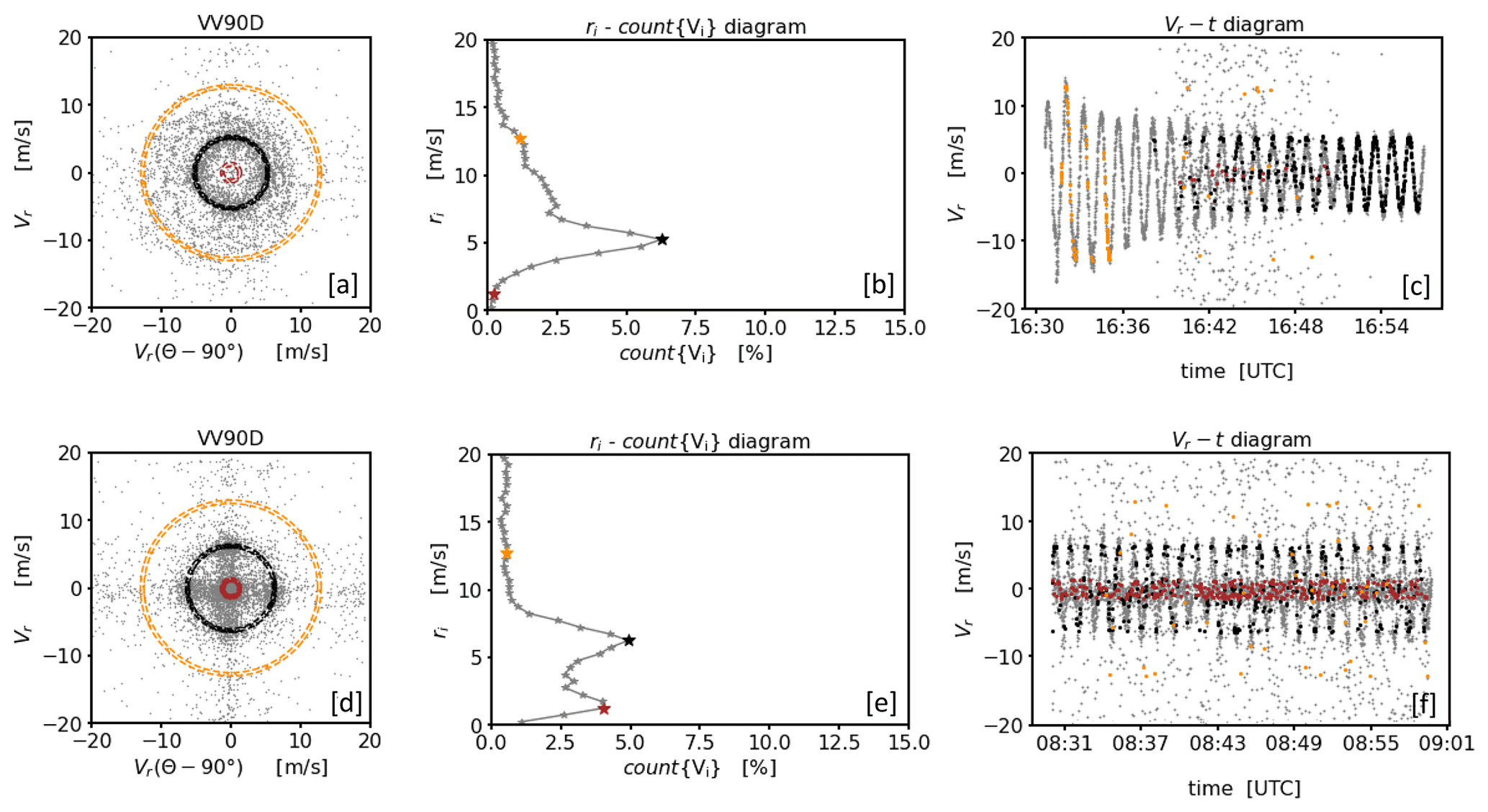
Figure 7 Examples of noise-contaminated DL measurements over a 30 min time period analyzed using the framework of the VV90D perspective. The upper (a–c) and lower (d–f) rows show measurements contaminated with type A and type B noise, respectively (see Fig. 1). The plots in each row show, from left to right, the VV90D plot (a, d), the frequency distribution binned by circular rings $r_i-\mathrm{\Delta }r\le r_i\le r_i+\mathrm{\Delta }r$, where $i=\mathrm{1},\mathrm{\dots },n$ (n∈ℕ) and with Δr=0.5 m s⁻¹ (b, e), and the time series plot (c, f). Additionally for each measurement example three specific circular rings have been chosen to illustrate where the measurement data contained in the circular ring (highlighted in different colors) are located in the time series plot.

4.2.1 Filtering by single point analysis – coarse filter I

One specific property emerging from the analysis of noisy DL data above is that if subsets V_i of data points binned by circular rings $r_i-\mathrm{\Delta }r\le r_i\le r_i+\mathrm{\Delta }r$ are analyzed individually, good estimates mostly occur in a dense sequence of points following the sinusoidal course of the measurements, while bad estimates mostly occur as singular points having no further data points in the immediate environment and take any value within the velocity space ±20 m s⁻¹. These properties open a first way for the development of a filter technique for bad estimates, namely,​​​​​​​ by detecting and discarding singular points in circular-ring-related subsets V_i of measurements. Practically, this can be implemented as follows. Use the framework of the VV90D perspective. Consider all circular rings spanning the VV90 plane individually. To select the ring-related data points, always start with the original time series and set all measurement points to a non-numeric flag value (e.g., NaN) which do not satisfy Eq. (4). This gives for each circular ring a certain ring-specific time series which has the length of the original one but where only measurement points are allocated with a numerical value which occur in the respective circular ring. Then, for each of the ring-specific time series sequentially check each position of the time series for flagged predecessor and successor positions within a pre-defined azimuthal environment. Positions occupied by an unflagged value, i.e., a numerical value, but with flagged predecessor and successor positions can be regarded as a singular point and discarded. Finally, the resulting circular-ring-related time series have to be merged back to one full time series which then represents a filtered time series where most of the bad estimates should be excluded. This filtering technique is referred to as coarse filter I hereafter. Note, however, that not all bad estimates necessarily occur as singular points. Hence, it is possible that a minor portion of bad estimates will still remain in the measurement series. Those can be discarded using classical outlier detection methods (e.g., the 3σ rule applied to differences of radial velocity measurements of two consecutive azimuthal measurement points) which are only effective if outliers are real outliers in the sense that they represent only a few unusual observations. In the case of noise-contaminated measurements the fraction of bad estimates is too high, which would not justify considering them to be outliers in the original sense.

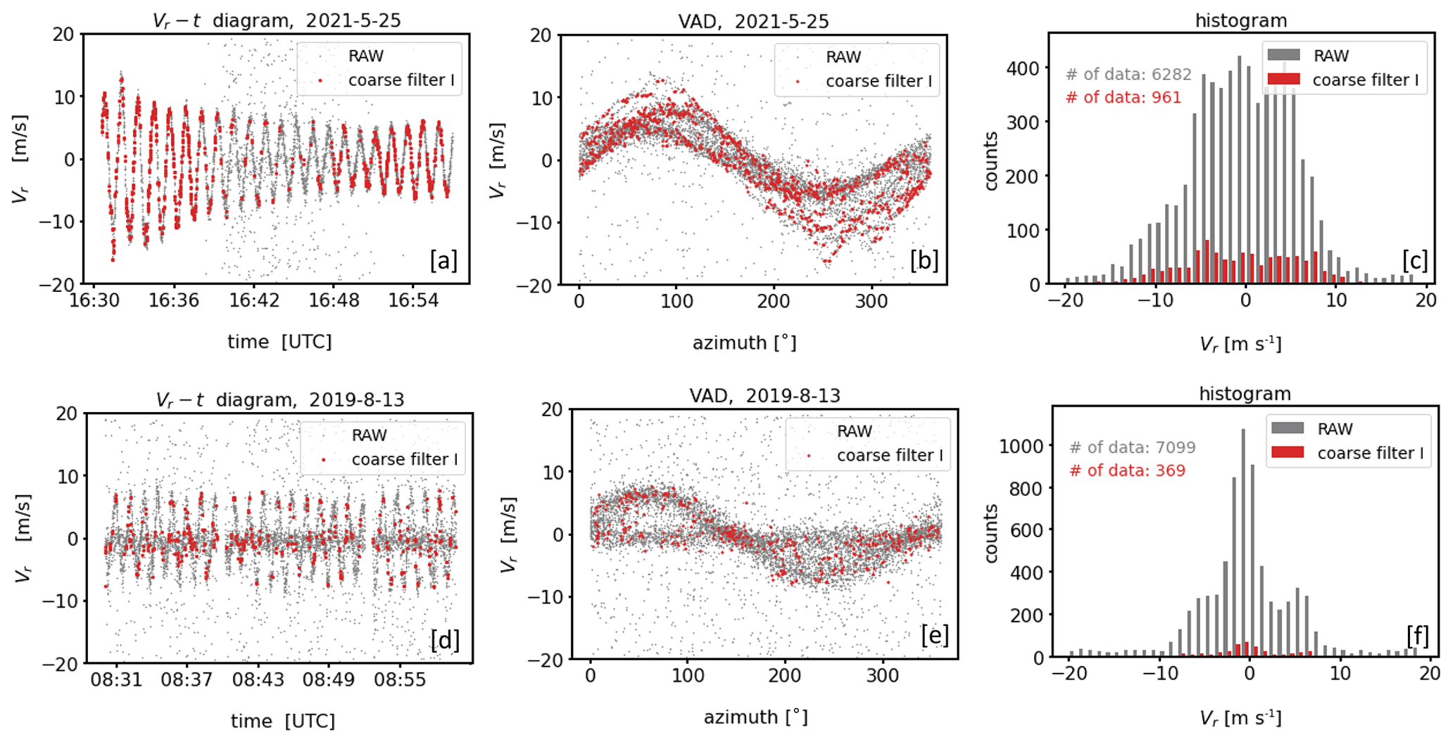
Figure 8 Examples of the outcome of coarse filter I. The upper (a–c) and lower (d–f) rows show measurements contaminated with type A and type B noise, respectively (see Fig. 1). The plots in each row show, from left to right, a comparison of the time series before (RAW) and after the application of coarse filter I using a V_r−t diagram (a, d), a comparison of the time series before and after filtering using the VAD perspective  (b, e), and a comparison of the associated histograms of the radial velocities (c, f).​​​​​​​

Results that can be obtained using coarse filter I applied to the measurement examples of Fig. 7 are shown in Fig. 8. It turns out that bad estimates can be best removed from measurements including type A noise (Fig. 8a). During the sub-interval of enhanced noise in the time series of the radial velocities, however, a severe thinning of data is striking, which reflects good estimates (Fig. 8b). This erroneous exclusion of good estimates happens when the number of measurement data, i.e., count{V_i}, is comparatively low for a larger number of circular rings. That is because low values of count{V_i} also mean that there is an increased probability that good estimates appear more frequently as singular points. Unfortunately, the latter makes the performance of coarse filter I weaker the more bad estimates are included in the time series of Doppler velocities (Fig. 8d, e) since an increased number of bad estimates increases the number of sparsely filled circular rings extending over the whole VV90 plane. From the VAD perspective, however, it can be seen that despite the strong data thinning the remaining data points represent a suitable first guess for good estimates of the time series which reveal the range of good estimates for each azimuthal direction (Fig. 8b). Considering the results of coarse filter I for the type B noise example the performance of the filtering technique is not convincing. Here, a huge fraction of bad estimates belonging to the type “noise around zero” remains in the dataset after applying the filtering method (Fig. 8e). From that we conclude that the specific distribution characteristics of type B noise measurements prohibit the possibility to distinguish between good and bad estimates by means of singular point detection.

4.2.2 Filtering based on ACF analysis – coarse filter II

The underlying idea of coarse filter II makes use of another specific property that can be derived from the analysis of noise-contaminated measurements using the framework of the VV90D perspective. It has already been described above that circular rings $r_i-\mathrm{\Delta }r\le r_i\le r_i+\mathrm{\Delta }r$ with a comparatively high data number count{V_i} mostly include good estimates and for circular rings with a decreasing data number the occurrence of bad estimates increases. Thus, it is to be expected that an evaluation of the ACF of circular-ring-related data subsets V_i with a high data number would yield ACF ($\mathit{\tau }=\mathrm{1};i$) ∼ 1. In contrast, for circular-ring-related data subsets V_i with a low data number this value would be comparably low (see Sect. 2.2 and Appendix B). This property opens up a second way for the development of a filter technique for bad estimates, namely by selecting only circular rings and the associated subsets of the entire time series of measurements with an ACF value not falling below a pre-defined threshold (ACF_thresh hereafter). Practically, this can be implemented as follows. Use the framework of the VV90D perspective. Seek in a first step that circular ring $r_i-\mathrm{\Delta }r\le r_i\le r_i+\mathrm{\Delta }r$ in the r_i−count{V_i} diagram with an absolute maximum in the data number (i.e., search for r_i with MAX(count{V_i}). Next, temporarily set all data points of the original measurement time series $V=V_{\mathrm{r}}(R,\mathit{\theta };t)$ to a non-numeric flag value (e.g., NaN) which do not satisfy Eq. (4) for the circular ring with the central radius r_i previously determined. This gives an initial guess for a filtered time series $V^{\mathrm{f}}=V_{\mathrm{r}}^{\mathrm{f}}(R,\mathit{\theta };t)$. To check for low noise contamination by means of the ACF, replace the flagged positions of the time series V^f with an estimated numerical value from the respective unflagged predecessor and successor positions using linear interpolation and calculate the ACF. The replacement of flagged positions is a necessary technical step to maintain the length of the time series and therewith the azimuthal distances between the single measurement points of the series. The latter is important since consecutive measurement data with different azimuthal distances would correlate differently with each other, which in turn would affect the ACF (see Appendix B). If the good quality of this filtered time series is reasonably assured, i.e., if ACF${}^{\mathrm{f}}(\mathit{\tau }=\mathrm{1})\sim \mathrm{1}$, the unflagged values of $V^{\mathrm{f}}=V_{\mathrm{r}}^{\mathrm{f}}(R,\mathit{\theta };t)$ can be regarded as reliable. In the same way as just described, by means of further iteration steps it is possible to gradually increase the number of reliable measurement data by repeating the above-described procedure taking not only the data from subsets V_i at circular rings $r_i-\mathrm{\Delta }r\le r_i\le r_i+\mathrm{\Delta }r$ with MAX(count{V_i}) into account but also those from adjacent circular rings $r_{i\pm \mathrm{1}}-\mathrm{\Delta }r\le r_{i\pm \mathrm{1}}\le r_{i\pm \mathrm{1}}+\mathrm{\Delta }r$, whereas the data number determines the order. This effectively results in the consideration of a wider circular ring with an accordingly higher number of data. The latter are constituents of a newly filtered time series $V^{{\mathrm{f}}_{\mathrm{new}}}=V_{\mathrm{r}}^{{\mathrm{f}}_{\mathrm{new}}}(R,\mathit{\theta };t)$ after the kth iteration. As long as the added subsets V_i±1 from adjacent circular rings include mostly good estimates, the associated ACF of the newly generated times series will remain close to 1, i.e., ACF${}^{{\mathrm{f}}_{\mathrm{new}}}(\mathit{\tau }=\mathrm{1})\sim \mathrm{1}$, and the iteration can be continued. The iteration has to be stopped if the ACF of the newly generated time series falls below a pre-defined threshold, i.e., if ACF${}^{{\mathrm{f}}_{\mathrm{new}}}(\mathit{\tau }=\mathrm{1})$ < ACF_thresh. That happens when the recently added data represent subsets of circular rings with an increased fraction of bad estimates. In this case, the result from the previous iteration step can be considered the best possible filtered time series with a maximum possible data availability and a low proportion of bad estimates at the same time. More detailed information useful for practical implementation of coarse filter II is given in Appendix F.

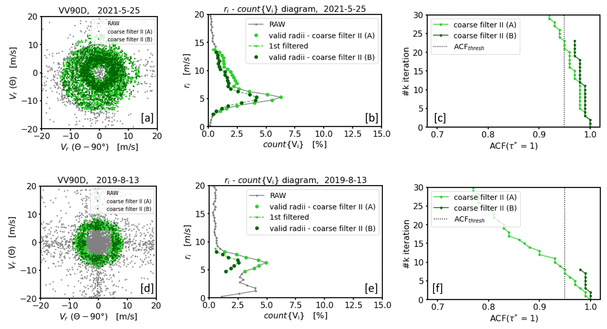
Figure 9 Example of the treatment of noise-contaminated DL measurements over a 30 min time period illustrated using the framework of the VV90D perspective in combination with intermediate results when coarse filter II has been applied. The upper (a–c) and lower (d–f) rows show measurements contaminated with type A and type B noise, respectively (see Fig. 1). The plots in each row show, from left to right, the VV90D plot (a, d), the frequency distribution binned by circular rings $r_i-\mathrm{\Delta }r\le r_i\le r_i+\mathrm{\Delta }r$, where $i=\mathrm{1},\mathrm{\dots },n$ (n∈ℕ) and with Δr=0.5 m s⁻¹ (b, e), and a graphic illustrating the change in the ACF with each iteration step (for more details see Sect. (4.2.2)). Additionally, intermediate results from two consecutive applications of coarse filter II, indicated by A and B, are shown.

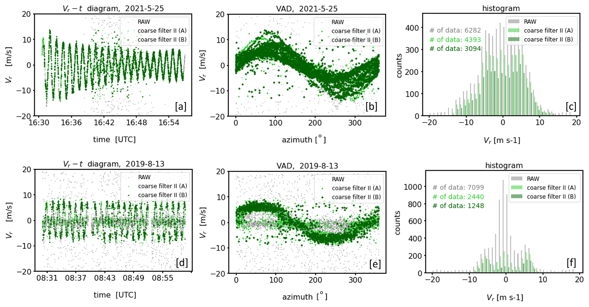
Figure 10 Examples of the outcome of coarse filter II. The upper (a–c) and lower (d–f) rows show measurements contaminated with type A and type B noise, respectively (see Fig. 1). The plots in each row show, from left to right, a comparison of the time series before (RAW) and after application of coarse filter II (a, d), a comparison of the time series before and after filtering using the VAD perspective (b, e), and a comparison of the associated histograms of the radial velocities (c, f).

For the measurement examples shown in Fig. 7 relevant technical details concerning coarse filter II are shown in Fig. 9. The change in ACF${}^{{\mathrm{f}}_{\mathrm{new}}}$ with each iteration step is illustrated in Fig. 9c and f. The circular rings included with each iteration step until the iteration has been stopped and the associated data points of the subsets V_i are color-coded in Fig. 9b and e and Fig. 9a and d, respectively. The final filter results of the measurement series that can be obtained using ACF_thresh=0.95 are shown in Fig. 10. The filter results based on coarse filter II differ from the results obtained based on coarse filter I (see Fig. 8) in two respects. One advantage of coarse filter II over coarse filter I is that fewer good estimates are incorrectly rejected, which is accompanied by a noticeably higher availability of good estimates. This can be verified based on the histograms comparing the distributions of the measurements from both the original and the filtered time series, which are shown in Figs. 8c and f and 10c and f, respectively. One disadvantage of coarse filter II over coarse filter I is that the hit rate of the filter goal of rejecting bad estimates is lower. This disadvantage of coarse filter II is more frequently observed for type A noise-contaminated measurements if the conditions during the measurement interval are nonstationary (see Fig. 10a–b) than for stationary intervals (not shown here). In this case an increase in the threshold value (e.g., ACF_thresh=0.99) would help to better remove bad estimates; however, this would be at the expense of removing more good estimates which describe the nonstationarity in the wind field. For type B noise-contaminated measurement intervals this issue also occurs for nonstationary measurement intervals (see Fig. 10d–e).

4.3 Post-processing filter for optimization

The coarse filter results presented in Sect. 4.2.1 and 4.2.2 are not yet satisfactory for the following reasons. Firstly, the frequently unjustified rejection of good estimates after applying coarse filter I results in an unnecessary reduction of reliable measurement data. Secondly, the number of remaining bad estimates after applying coarse filter II is still too high. Hence, additional efforts are required to further optimize the filter results. Therefore, the results of coarse filters I and II will be treated as intermediate results only at this point. Possible further optimization steps are considered in more detail next. The entirety of these steps represents the filter for post-processing. Note that all analyses are from now on carried out using the VAD perspective.

4.3.1 Two-stage MAD filter

The median absolute deviation (MAD) is a well-known statistical tool for outlier detection in measured datasets (Iglewicz and Hoaglin, 1993) having a unimodal and symmetrical distribution (see Sect. 3). Here, the MAD is used as an additional filter step following coarse filter II. The term “outlier” refers to a few uncontrollable and abnormal observations which seem to lie outside the considered population. If $X=\mathit{\{}{x}_{\mathrm{1}},x_{\mathrm{2}},\mathrm{\dots },x_n\mathit{\}}$, with n ∈ℕ, is a given dataset of measurements that is normally distributed (i.e., 𝒩(μ, σ²) with mean μ and variance σ² ), the MAD is defined through

$$\begin{array}{}\text{(5)}& \mathrm{MAD}=\mathrm{median}\left(\right|x_i-\mathrm{median}\left(X\right)\left|\right).\end{array}$$

According to Iglewicz and Hoaglin (1993), values x_i are regarded as outliers if they are not included in an interval given by

$$\begin{array}{}\text{(6)}& \mathrm{median}\left(X\right)-q{\displaystyle \frac{\mathrm{MAD}}{\mathrm{0.6745}}}\le x_i\le \mathrm{median}\left(X\right)+q{\displaystyle \frac{\mathrm{MAD}}{\mathrm{0.6745}}}.\end{array}$$

The cut-off value q is mostly chosen arbitrarily. Iglewicz and Hoaglin (1993) suggest q=3.5. A modification of the MAD is the so-called double MAD, which can be used for nonsymmetric distributions (Rosenmai, 2013). The MAD outlier detection method works in analogy to the 3σ rule of thumb (Gränicher, 1996) but is classified as the more robust one. Robust in this context means that the median and MAD itself are less affected by outliers than the mean or the standard deviation σ. Having this in mind, care has to be taken when applying the MAD method to DL radial velocity measurements including a huge fraction of bad estimates. In such a case bad estimates can no longer be considered only a few unusual observations and it is not unlikely that the median is also influenced by them so that the requirements for an application of the MAD are no longer met. For this reason, the MAD is only used here as a post-processing filter for DL measurements that were previously filtered with coarse filter II.

Looking at the pre-filtered DL measurements from the VAD perspective (Fig. 10b, e), the application of the MAD outlier detection method is followed in two steps. In the first stage (MAD_part_I, hereafter) we apply the MAD azimuth-wise, i.e., to datasets representing measurements from only one direction. In the second stage (MAD_part_II, hereafter) we apply the MAD to a dataset representing squared deviations $(V_{\mathrm{r}}-V_{\mathrm{r}}^{\mathrm{FSWF}}{)}^{\mathrm{2}}$ of radial velocity measurements V_r from sine wave fit radial velocities $V_{\mathrm{r}}^{\mathrm{FSWF}}$. In order to determine the latter the so-called filtered sine wave fit (FSWF) as a wind vector estimation technique introduced by Smalikho (2003) has been used. This technique requires knowledge about the standard deviation σ of good estimates which has been estimated based on the filter results of MAD_part_I. Intermediate results of the two-stage MAD applied to the outcome of coarse filter II (Fig. 10b) are illustrated in Fig. 11. From our experience we know that employing MAD_part_I, particularly by means of the double MAD filter technique (Rosenmai, 2013), may contribute to retain the azimuthal variability in V_r. The latter is important, especially when the wind field was inhomogeneous and nonstationary during the 30 min measurement interval. This can be seen in Fig. 11a, illustrating the outcome of MAD_part_I. Here, relevant measurements reflecting the nonstationarity of the wind field still remain in the filtered dataset even if they deviate substantially from the rest of the azimuthal dataset, as can be seen, for instance, around the azimuth angles θ=80° and θ=250°. However, it is also noticeable in Fig. 11b that after applying MAD_part_I not all bad estimates could be removed from the dataset. This can be explained by the fact that often not enough data per azimuth sector were available for a reliable calculation of the median and MAD. For that reason MAD_part_II becomes necessary to further improve the bad estimate detection rate. Corresponding filter results are illustrated in Fig. 11b and clearly show that the fraction of remaining bad estimates could be substantially reduced. Unfortunately, MAD_part_II also contributes to a severe cut-off of a huge fraction of directional variability which was actually possible to avoid by applying MAD_part_I. This can be attributed to the choice of the cut-off (here: q=3.5) and very clearly shows the fundamental issues when using statistical filter methods where cut-off values have to be carefully chosen and cannot be generalized as would be required for a routine application.

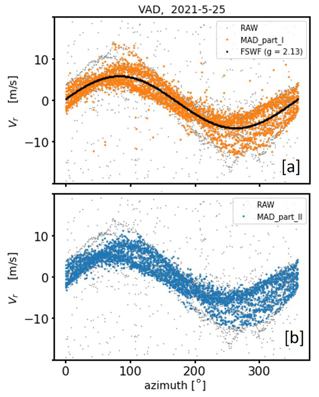
Figure 11 Intermediate results of the two-stage MAD filter applied to the outcome of coarse filter II for the type A measurement example shown in Fig. 10b. The outcome of MAD_part_I and MAD_part_II is shown in panels (a) and (b), respectively. Furthermore in panel (a) the results of a filter sine wave fit (FSWF) are shown, which has been calculated based on a standard deviation (here $\mathit{\sigma }=g=\mathrm{2.13}$ m s⁻¹) obtained from the colored data reflecting the results of MAD_part_I.

4.3.2 Determination of the sinusoidal corridor of good estimates

The main advantage of coarse filter I over coarse filter II is the better performance with respect to the detection of bad estimates, which makes the two-stage MAD filter as a follow-up filter step of coarse filter I redundant at this point. The disadvantage of coarse filter I, however, lies in the strong rejection of many obviously good estimates (see Sect. 4.2.1). Next a possibility is described regarding how to reverse wrong data rejection decisions in order to increase the availability of reliable measurements again.

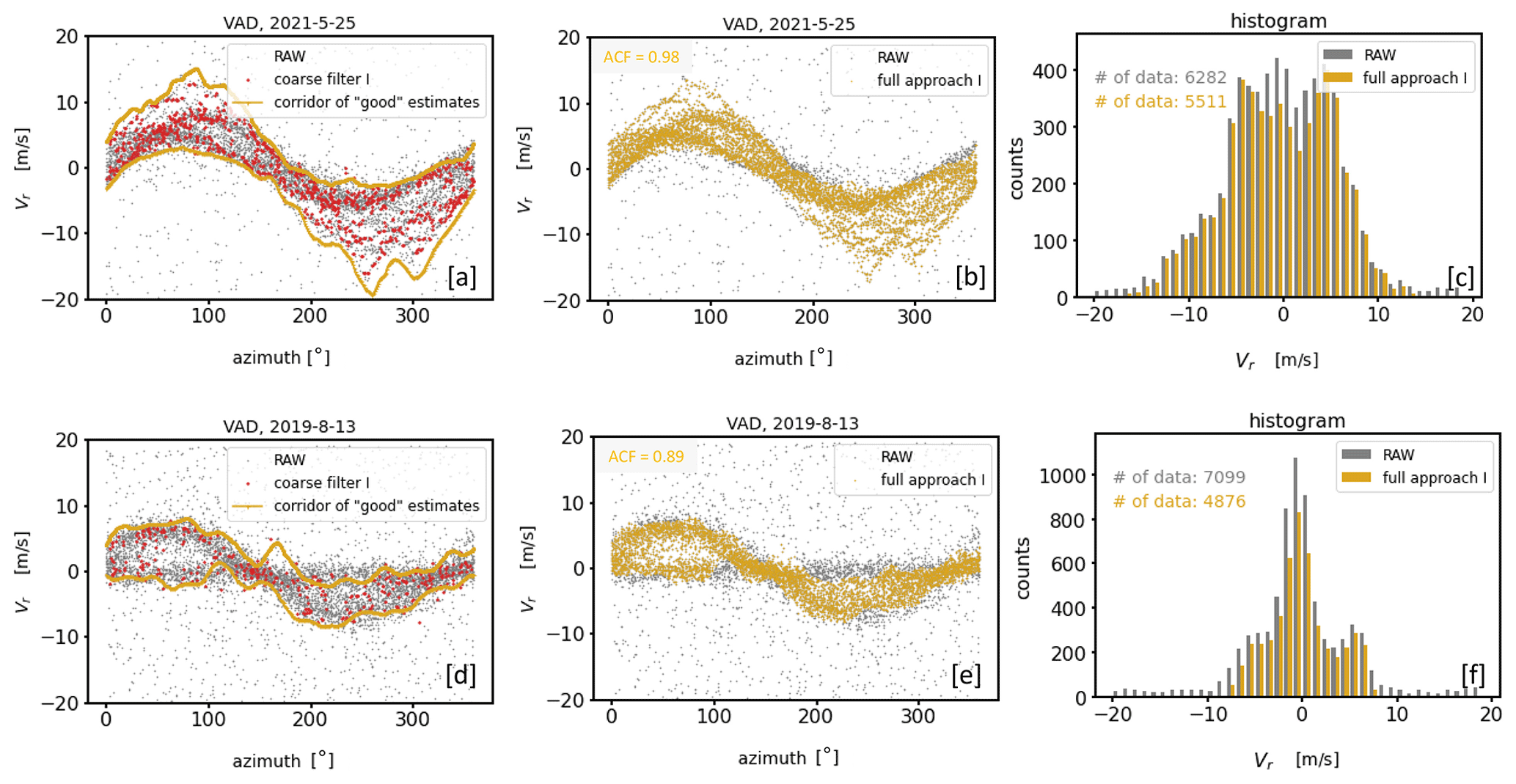
Figure 12 Results of the filter for post-processing applied to the outcome of coarse filter I (see Fig. 8) for two measurement examples characterized by a different type of noise distribution (top: type A noise, bottom: type B noise). The panels in each row show, from left to right, the identified borders of the area which defines the corridor of good estimates (a, d), the outcome of the re-activation step of previously discarded good estimates (b, e), and the associated histograms which provide an overview of the final data availability of V_r estimates identified as good data (c, f).

It has been shown in Sect. 4.2.1 that the outcome of coarse filter I for noise-contaminated measurements of type A (Fig. 8a–c) is a dataset representing a suitable first guess for good estimates if visualized using the VAD perspective (Fig. 8b). Hence, the roughly filtered data can be used to narrow down the sinusoidal area in the VAD space where most of the good estimates can be found. This in turn offers the possibility to re-activate radial velocities within the area boundaries as good data that were discarded after applying coarse filter I. The outcome of such a re-activation as a post-processing step of coarse filter I is shown in Fig. 12. The identified borders of the area which define the corridor of good estimates shown in Fig. 12a and d have been determined in the following two consecutive steps: firstly by calculating the min and max radial velocity values for each azimuthal direction and secondly by calculating the upper envelope of the max values and the lower envelope of the min values over the interval 0 to 360°. Then the re-activation of falsely rejected good estimates is done by considering all measurement points within the corridor defined by the upper and lower envelopes to be good estimates. The corresponding results of this step are shown in Fig. 12b and e. Note that the procedure described above to determine the area of good estimates is relatively simple and has its weaknesses, especially in the case of low data availability, which complicates the determination of the envelope due to a small number of available min and max values. For such conditions a more sophisticated approach is needed. The re-activation results for the measurement example characterized by type A noise shown in Fig. 12b match the data one would identify as good data well from a visual point of view. Furthermore, the re-activation step is accompanied by a strong increase in reliable data compared to the outcome of coarse filter I (compare Figs. 8c and 12c). Hence the higher data availability achieved in this way may contribute to an improvement of the variance statistics required for a turbulence product retrieval. In contrast, the re-activation step fails if applied to type B noise-contaminated measurements, which is shown in Fig. 12e. This is due to both the poor first-guess results for good estimates after applying coarse filter I, which does not contain enough details to correctly narrow down the sinusoidal area of good estimates, and some of the remaining bad estimates that belong to the specific class of noise around zero. Note that to discard the latter, here we omitted the two-stage MAD as a follow-up filter of coarse filter I. This is because we know from our experience that the generally significantly lower data availability of reliable measurement data after the application of coarse filter I compared to coarse filter II turns out to be unfavorable for a successful MAD application.

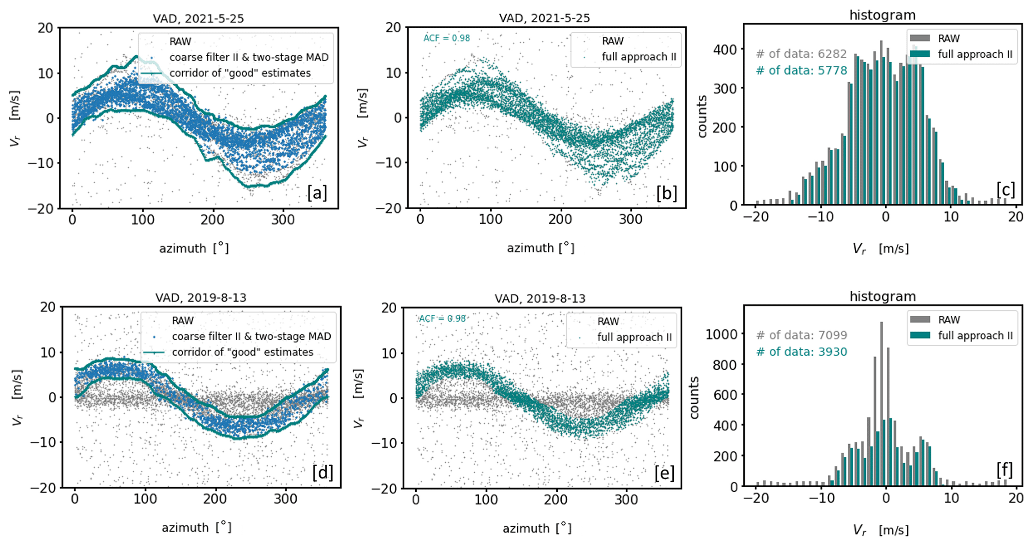
Figure 13 Results of the filter for post-processing applied to the outcome of coarse filter II in combination with a follow-up two-stage MAD filter step (see Figs. 10 and 11) for two measurement examples characterized by a different type of noise distribution (top: type A noise, bottom: type B noise). The panels in each row show, from left to right, the identified borders of the area which defines the corridor of good estimates (a, d), the outcome of the re-activation step of previously discarded good estimates (b, e), and the associated histograms which provide an overview of the final data availability of good estimates (c, f).

So far the re-activation step of falsely rejected good estimates introduced above has been discussed in the context of a post-processing of filter results after applying coarse filter I. Even if an unjustified data loss of good estimates after an application of coarse filter II is not that substantial the above-described re-activation step can also be applied to the outcome of coarse filter II. However, for the reasons mentioned in Sect. 4.3.1 this requires a previously executed two-stage MAD filter. The corresponding results are shown in Fig. 13 where the significantly better results for the type B noise example (Fig. 13d–f) are obvious. The disadvantage, however, is that with the re-activation step a substantial number of bad estimates in the region around the reflection point of the sinusoidal corridor of good estimates is also assigned to the set of good data. At this point the corridor of good estimates and the horizontal band reflecting a higher concentration of noise around zero overlap, and no clear distinction between good and bad estimates is possible. This can also be seen by comparing the histograms shown in Figs. 10f and 13f.

Finally, it should be mentioned that with the re-activation of initially discarded data in the identified corridor of good estimates there is always a risk of returning a certain number of bad estimates if the raw measurements were contaminated with noise. Since bad estimates can be distributed over the whole measurement space of ±19 m s⁻¹ they potentially also occur in the corridor of good estimates. However, as long as the interest is only in mean wind and turbulence statistics, which are primarily obtained using the VAD perspective, the effect of such a small fraction of bad estimates is expected to be negligible.

4.4 Intercomparison of approach I and approach II under different atmospheric wind conditions

In the previous subsections the limits of the usability of approach I and approach II depending on the type of noise have been discussed. The type of noise, however, is not the only factor affecting the applicability of the two different filtering techniques. Their success is also linked to the strength and temporal evolution of the wind during the measurement period. This becomes obvious by comparing the filter results of approach I and approach II for both type A and type B noise (Figs. 14 and 15) while considering the following categories: (I) weak and stationary wind, (II) strong and stationary wind, (III) weak and nonstationary wind, and (IV) strong and nonstationary wind.

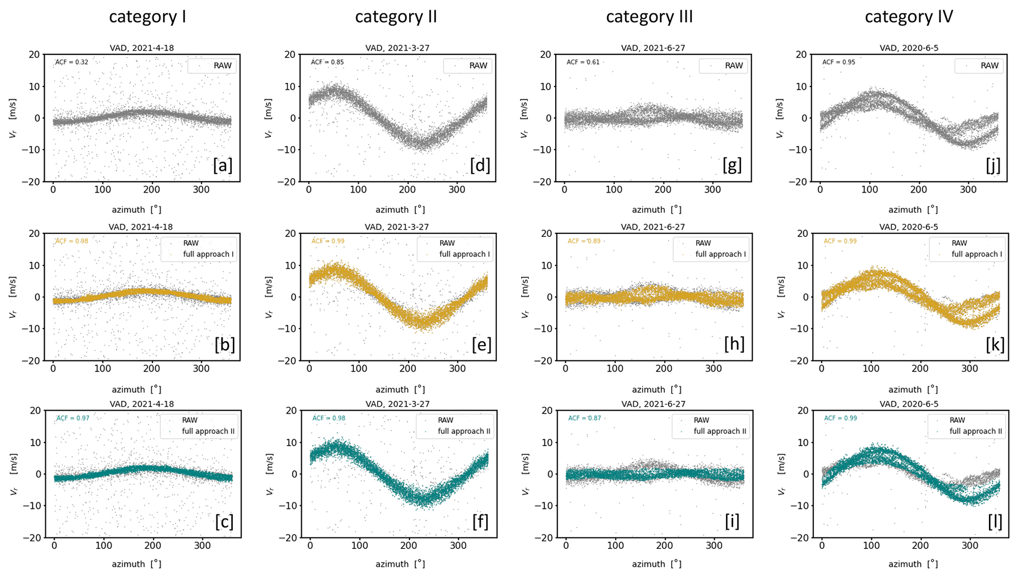
Figure 14 Overview of the final filter results of approach I and approach II for DL measurement examples contaminated with type A noise. The examples of each column represent four selected atmospheric conditions with respect to the wind situation: weak and stationary wind (category I), strong and stationary wind (category II), weak and nonstationary wind (category III), and strong and nonstationary wind (category IV). The panels in the first row show the time series of the respective RAW data of the DL radial velocity measurements over a measurement interval of 30 min. The panels in the second (third) row show both the RAW data and the filter results of approach I (approach II) in different colors.

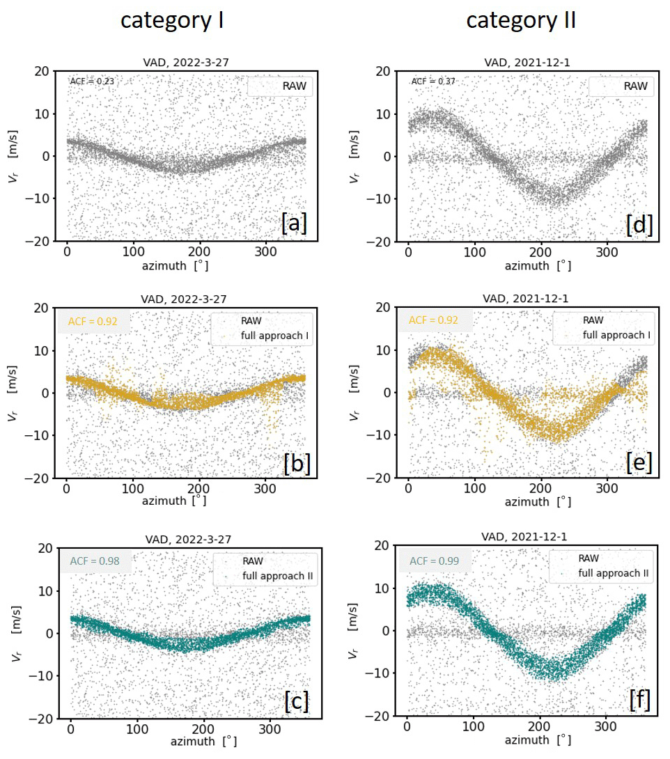
Figure 15 Same as in Fig. 14 except that DL measurements contaminated with type B noise are considered. Categories III and IV are not available.

Comparing the filter results for measurements with type A noise the outcomes of approach I and approach II are equally good for category I and II (Fig. 14b, e and c, f), but for category III and IV the results based on approach I (Fig. 14h, k) turn out better than based on approach II (Fig. 14i, l). The differences in the results for category III and IV are not because bad estimates have not been correctly detected by approach II but rather due to the wrong rejection of a substantial number of obviously good estimates. This error can be traced back to a bimodal distribution in the measurement-related r_i−count{V_i} diagram (not shown) caused by the nonstationarity of the wind field during the 30 min measurement interval. Here, the secondary peak was incorrectly interpreted as noise around zero (see Sect. 4.2.2). Note that coarse filter II of approach II is not designed to make this distinction and thus fails when applied to situations belonging to category III and IV. In contrast, when comparing the filter results for type B noise measurements (Fig. 15) approach II is better than approach I for category I and II. This can be seen not only visually but also numerically by means of the ACF. While the ACF values were between 0.23 and 0.37 in the unfiltered time series (Fig. 15a, d), after applying the filtering technique the ACF takes values between 0.98 and 0.99 for approach II (Fig. 15c, f) but only values around 0.92 for approach I (Fig. 15b, e). Finally, two more findings are considered worth mentioning here: firstly, measurements during wind conditions belonging to category III are obviously difficult to manage for both approaches, indicated by the comparably poor ACF values of the fully filtered time series in a range between 0.87 and 0.89 (Fig. 14h, i). Secondly, it becomes obvious that, particularly during weak wind conditions (i.e., category I and III), the bands of good estimates sometimes seem too narrow from a purely visual point of view. This observation holds for both of the filter approaches (Fig. 14b, c and h, i). The reason for this lies in the method to determine the envelope in connection with the final re-activation step of previously discarded good estimates (see Sect. 4.3.2). As a result, some information on the actual variability is lost in the filtered dataset. This in turn may result in an underestimation of variances as will be shown in Sect. 5.1.

Knowledge and insights gained from the overview given in this section are important to develop a strategy to implement the filtering techniques for operational use. More detailed information on a strategy that can be used for an implementation of approach I and approach II is given in Appendix G.

5 Turbulence retrieval based on pre-processed DL measurements using traditional and the new filter technologies

Depending on the filtering technique used, the decision about which of the radial velocities are classified as good or bad estimates can turn out very differently. Hence, it is to be expected that differently pre-filtered DL measurements may result in differences in the retrieved turbulence variables. This section aims to demonstrate that due to the higher sensitivity of the newly introduced filtering techniques concerning both the rejection of bad estimates and the acceptance of good estimates, the quality and data availability of DL-based turbulence measurements (e.g., TKE retrieved following Smalikho and Banakh, 2017) can be improved. For DL measurements with a probability of bad estimates close to zero this method delivers reasonable results (see Appendix H). Thus, if differently pre-filtered DL data are used as input for the retrieval process, large errors in the retrieved TKE can be attributed to either a faulty noise filtering that leaves bad estimates in the filtered dataset or to an overfiltering that removes too many reliable data points.

5.1 Comparisons with sonic anemometer as an independent reference

In order to be able to assess the quality of TKE variables based on differently pre-filtered DL measurements, as an independent reference, sonic data from a 99 m tall meteorological mast are used. The measurements were performed with a USA-1 sonic anemometer (Metek GmbH) at a sampling rate of 20 Hz, and the raw data were processed with EddyPro (LiCor Inc.) software. The mast is operated at GM Falkenberg at a distance of about 80 m towards SSW from the DL system.

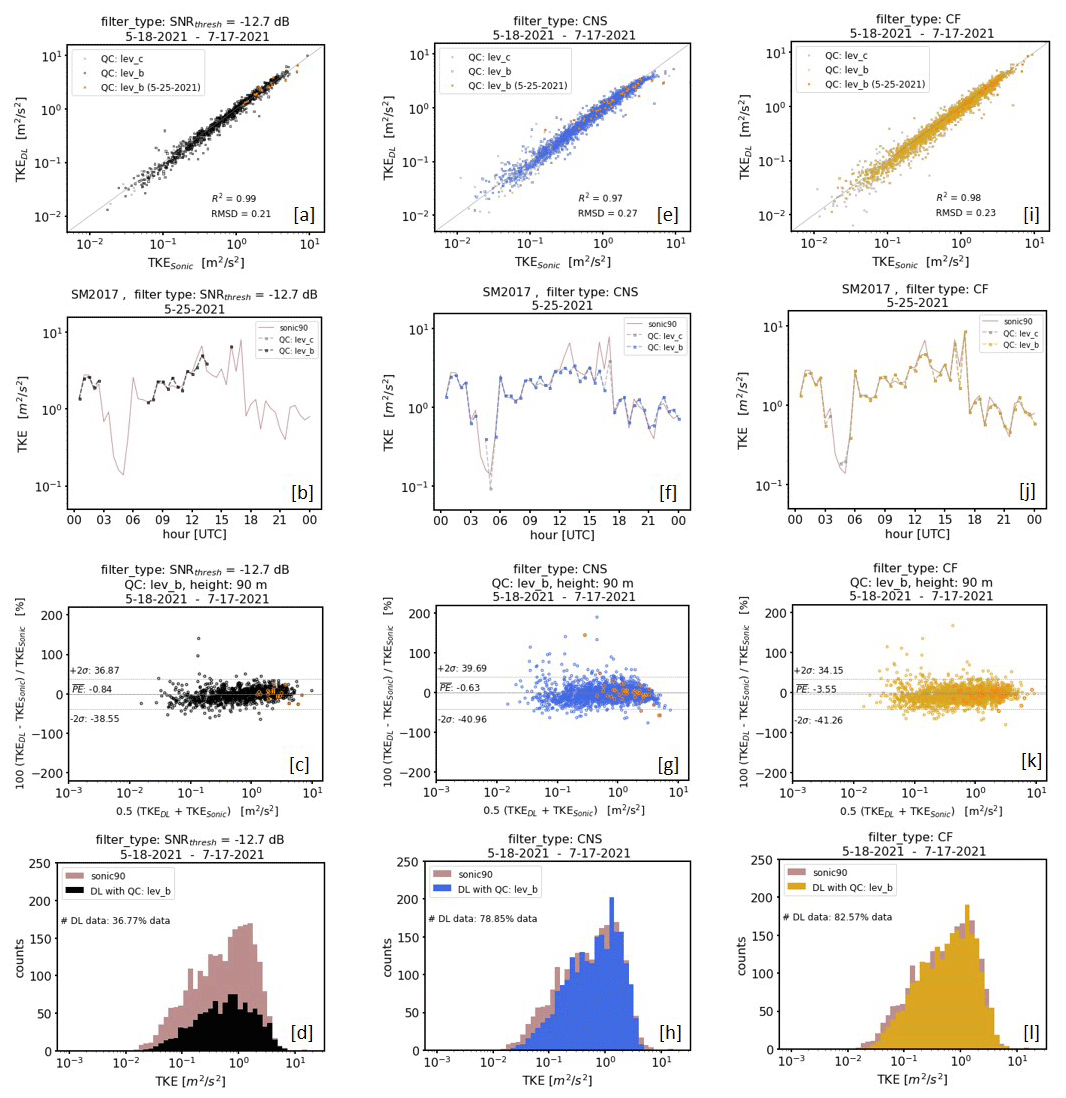
Figure 16 Comparison of Doppler-lidar-based TKE at 95 m height with data from a mast equipped with a sonic device at 90 m height. The measurement period was from 18 May to 17 July 2021. Each column represents the comparison of different TKE products based on differently pre-filtered input data. SNR threshold filtered data with SNR_thresh = −12.7 dB and consensus (CNS) filtered data have been used in the left and middle column, respectively. Input data obtained using a combined filter (CF) application of approach I and approach II have been used in right column. The panels of each column represent comparisons between DL and sonic data using different visualization techniques. These are, from top to bottom, scatterplots, time series plots (1 d only, 25 May 2021), Bland–Altman plots, and histograms. The abbreviation “QC: lev_x” in the scatterplots (a, e, i) refers to different levels of product quality control (see Sect. 5.1).

Results of an intercomparison of TKE retrievals based on differently pre-filtered DL data versus sonic TKE measurements are summarized in Fig. 16. Three different cases are analyzed: TKE retrievals calculated by means of (i) SNR-threshold-based filtered input data using SNR_thresh = −12.7 dB (Fig. 16a–d), (ii) CNS-based filtered data (Fig. 16e–h), and (iii) CF-based filtered data (Fig. 16i–l). Here CF (combined filter) stands for a combined application of approach I and approach II because of the occurrence of type A and type B noise in the DL78 measurements (see Sect. 2.1–2.2 and Appendix G). For each case an additional distinction is made between TKE products which are subject to different quality control (QC) steps. Here, the minimum requirement for a TKE value representing a 30 min mean is that its retrieval is based on more than 60 % of reliable measurements of V_r during the measurement interval (lev_c hereafter). Since the TKE reconstruction method relies on a variety of theoretical assumptions (e.g., see Eq. 22 in Smalikho and Banakh, 2017) a further QC step proves the fulfillment of these requirements (lev_b hereafter). To obtain meaningful results the evaluations are based on a 2-month dataset of DL measurements at GM Falkenberg which were collected during () from 18 May to 17 July 2021.

Considering the Doppler lidar TKE retrieval based on a pre-filtering of the measurements using the SNR threshold approach, the problems that arise in connection with routine turbulence measurements (see Sect. 1) can be supported here numerically. Although good data quality is achieved compared to sonic measurements (R² = 0.99 and RMSD = 0.21; Fig. 16a), data availability is very low (36.77 %; Fig. 16d). TKE values based on CF pre-filtered DL data have almost comparable data quality (R² = 0.98 and RMSD = 0.23; Fig. 16i) but score additionally with a significantly higher data availability (82.57 %; Fig. 16l). TKE results based on CNS pre-filtered DL data are also characterized by a higher data availability (78.85 %; Fig. 16h) but have poorer data quality (R² = 0.97 and RMSD = 0.27; Fig. 16e). To explain the latter, the time series plot comparisons between DL data and sonic data displayed in Fig. 16b and f for the example day 25 May 2021 are helpful. This day is a typical example day with noise-contaminated DL measurements over the whole day but with an obvious higher density of bad estimates in the early morning between 04:00 and 07:00 UTC and in the afternoon from 16:00 UTC onwards (see Fig. H1, 2 – Appendix H). Note that during these time intervals no reliable TKE values are available if an SNR threshold pre-filtering is used. In contrast, using CNS pre-filtered data, retrieved TKE values are available for these time periods, which, however, are partly subject to errors if compared with sonic data. For instance, DL-based TKE values obtained at 04:30 and 16:00 UTC show either a pronounced overestimation or underestimation if compared with sonic-based TKE measurements. With a closer look into the DL radial velocity measurements from which these 30 min TKE values have been retrieved, this overestimation and underestimation can be easily explained (see Fig. 5b, d). For the measurement period between 04:00 and 04:30 UTC the prescribed search interval ΔV_r=3 m s⁻¹ was too large so that bad estimates remained in the dataset and introduced an additional variance contribution, yielding an overestimation of the TKE. For the measurement period between 15:30 and 16:00 UTC the value for ΔV_r was too small so that relevant features of the wind field were not captured. As a consequence, the dataset and thus the derived variances are not representative for the 30 min measurement interval, yielding an underestimation of the TKE value. These examples clearly show the weaknesses of the CNS filtering technique if the ΔV_r search interval is inadequately selected. With a fixed ΔV_r during $\mathrm{24}/\mathrm{7}$ routine measurements such situations occur quite frequently, which explains why the data quality of TKE values retrieved from CNS pre-filtered DL data is worse compared to TKE retrieved from pre-filtered DL data using the SNR thresholding technique. Note that with the newly introduced CF filtering technique the above-described issues can be avoided and therewith more reliable TKE values can be derived (Fig. 16j, l).

One additional interim note should be given on the high sonic TKE value of ∼ 7 m² s⁻² at 16:00 UTC (Fig. 16f). This value is likely caused by an instationary wind field during the 30 min measuring interval rather than due to eddies in the turbulent flow. For that reason this value should be flagged as non-reliable. The problem, however, is that with the CNS filtering technique relevant wind information characterizing this nonstationarity would be rejected so that the identification of such nonstationarity would not be possible.

Another way to compare TKE variables retrieved from differently pre-filtered DL measurements is based on the use of a so-called Bland and Altman plot (Fig. 16 c, g and k). This kind of plot was introduced by Bland and Altman (1986) to statistically assess the comparability between two measurement methods. The advantage of this statistical evaluation method is that it not only provides insight into systematic deviations (bias) and limits of agreement but also reveals how the differences between two measurement methods depend on the magnitude of the measurement value. For the Bland–Altman plots shown in Fig. 16 c, g, and k, the y axis shows the percentage error (PE) between two paired measurements, i.e., $\mathrm{100}\times ({\mathrm{TKE}}_{\mathrm{DL}}-{\mathrm{TKE}}_{\mathrm{Sonic}})/{\mathrm{TKE}}_{\mathrm{Sonic}}$, and the x axis represents the average of these values, i.e., (${\mathrm{TKE}}_{\mathrm{DL}}+{\mathrm{TKE}}_{\mathrm{Sonic}})/\mathrm{2}$. Additionally, the horizontal lines indicate the mean percentage error ($\stackrel{\mathrm{‾}}{\mathrm{PE}}$) and twice the standard deviation (±2σ) from the mean. The latter denotes the statistical limits of agreement. For the Bland–Altman plot shown in Fig. 16c the mean percentage error is close to zero ($\stackrel{\mathrm{‾}}{\mathrm{PE}}$ = −0.84 %). This indicates that there are hardly any systematic differences between DL-based TKE retrievals using the SNR threshold method for noise filtering and sonic-based TKE measurements. Additionally it can be seen that there is a nearly symmetric distribution of the paired points around the horizontal line denoting $\stackrel{\mathrm{‾}}{\mathrm{PE}}$, with a slight tendency towards a more frequent underestimation by the DL for small TKE values and a more frequent overestimation for higher TKE values. As a result, in 95 % of the cases the DL delivers a TKE value that is up to 39 % smaller or up to 37 % larger than the one measured by the sonic anemometer. With the exception of an offset of about 2.7 % in bias and the limits of agreement, qualitatively similar results can be derived when comparing DL-based TKE retrievals using the CF filter with sonic-based TKE (Fig. 16k). The Bland–Altman comparisons for DL-based TKE values using the CNS filter reveal less good correspondence (Fig. 16g). Although the mean percentage error ($\stackrel{\mathrm{‾}}{\mathrm{PE}}$ = −0.63 %) does not significantly differ from the results shown in Fig. 16 c, the range between the limits of agreement is larger ($\stackrel{\mathrm{‾}}{\mathrm{PE}}\pm \mathrm{2}\mathit{\sigma }=\mathit{\{}+\mathrm{40}\mathit{\%},-\mathrm{41}\mathit{\%}\mathit{\}}$). Furthermore, a slightly different point cloud distribution can be seen. Especially for larger TKE values there seems to be a greater underestimation of DL-based TKE retrievals compared to sonic TKE.

5.2 Comparisons with alternative reference data

With increasing altitudes the probability of bad estimates in DL radial velocity measurements increases. This is due to the typically decreasing aerosol density, which is also noticeable in weaker SNR values. Therefore, the actual robustness of the filtering methods can be tested much better at larger measuring heights, where the methods have to cope with an increased occurrence of noise. Unfortunately, the tower-based measurements at GM Falkenberg are only provided up to 99 m height so that for higher altitudes no independent references for a comparison are available. For that reason an alternative way based on the following strategy is used. In the subsequent analysis, DL TKE values obtained using the SNR threshold method for noise filtering are used as an alternative reference intended to replace the missing sonic data at higher altitudes. This can be motivated by two arguments. On the one hand, it could be shown that the comparison of TKE values based on SNR pre-filtering with independent sonic data provided the best results (see Fig. 16). On the other hand the SNR thresholding approach is a standard method to exclude bad estimates from DL measurements. For that reason confidence in the validity of TKE products based on SNR pre-filtering is very high and TKE products based on differently pre-filtered input data should be comparable by similar performance of the filtering method.

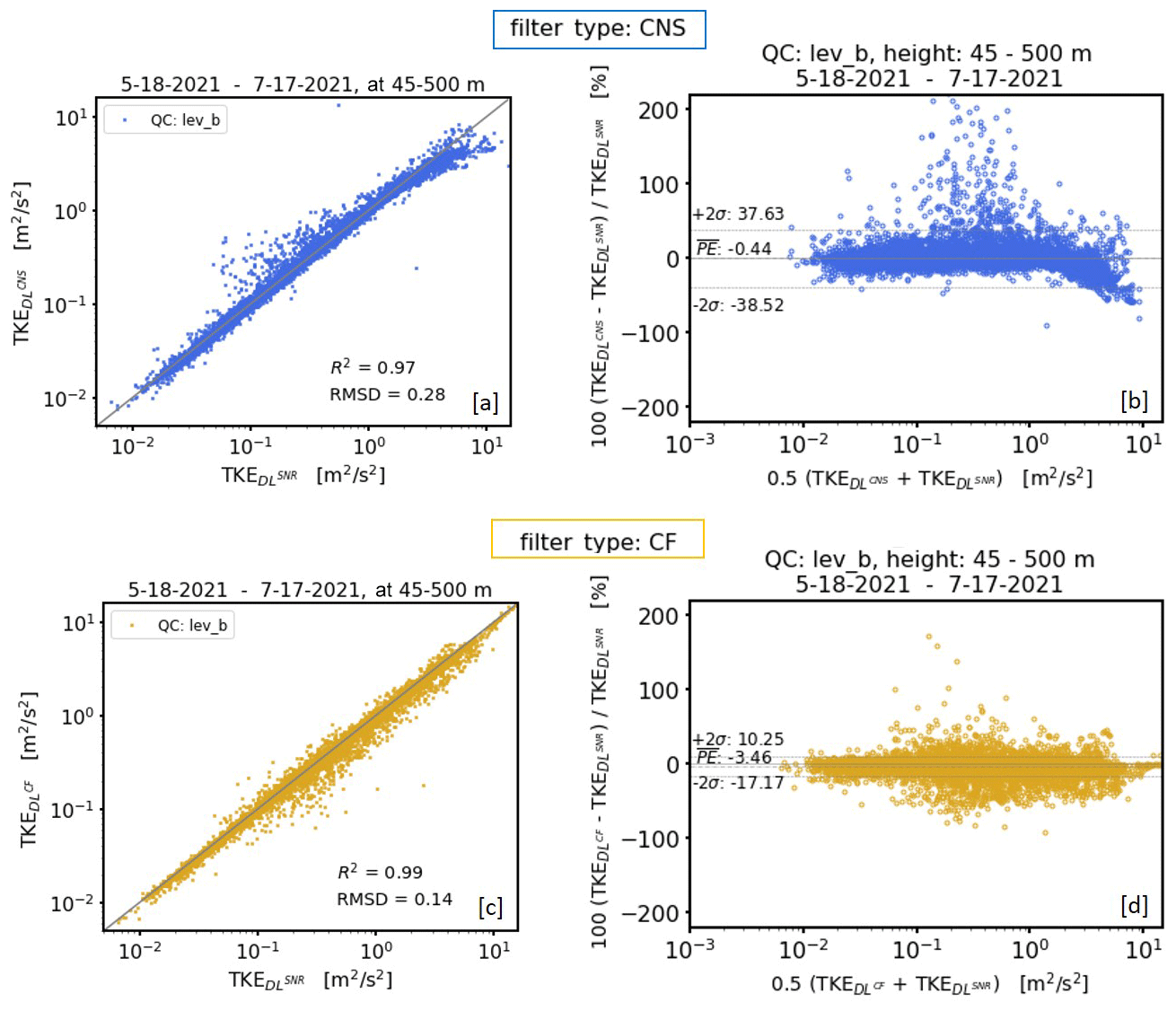
Figure 17 Comparison of TKE from DL based on differently pre-filtered measurement data prior to the TKE retrieval as proposed in Smalikho and Banakh (2017). Scatterplot (a) showing TKE products based on CNS pre-filtering (TKE${}_{{\mathrm{DL}}^{\mathrm{CNS}}}$) against TKE products based on a pre-filtering using the SNR thresholding technique (TKE${}_{{\mathrm{DL}}^{\mathrm{SNR}}}$) with SNR_thresh = −12.7 dB. Similarly, scatterplot (c) showing TKE products based on CF pre-filtering (TKE${}_{{\mathrm{DL}}^{\mathrm{CF}}}$) against TKE products based on a pre-filtering using the SNR thresholding technique. The scatterplots include all available DL measurements up to 500 m height over a measurement period from 18 May to 17 July 2021. In analogy, the same applies for the Bland and Altman (BA) plots (b, d). Here, the relative percentage difference between TKE${}_{{\mathrm{DL}}^{\mathrm{CNS}}}$ (TKE${}_{{\mathrm{DL}}^{\mathrm{CF}}}$) and TKE${}_{{\mathrm{DL}}^{\mathrm{SNR}}}$ products is plotted against its mean value. For more details concerning BA plots see Sect. 5.1.

Comparisons of TKE products based on SNR pre-filtered DL data with those based on CNS filtering and CF filtering for measurement heights between 45 and 500 m are shown in Fig. 17a–b and c–d, respectively. There are two obvious issues with the CNS filtering that become apparent in Fig. 17a and b: on the one hand, the clear underestimation of larger DL-based TKE values for values above 2 m² s⁻² and, on the other hand, the occurrence of a significant number of strongly overestimated TKE values in a range of 0.06 m² s⁻² < TKE < 0.5 m² s⁻². These errors are caused by the deficiencies of the CNS filter method already described in Sect. 3.2, i.e., an inappropriate choice of the search interval ΔV_r. In contrast, the comparisons shown in Fig. 17c and d reveal better agreement between TKE retrievals based on SNR pre-filtered DL data with those based on CF filtering. This is evident from both a visual and statistical perspective. For instance, the higher sensitivity of the CF filter with respect to the rejection of bad estimates and the acceptance of good estimates contributes with $\stackrel{\mathrm{‾}}{\mathrm{PE}}\pm \mathrm{2}\mathit{\sigma }=\mathit{\{}+\mathrm{10}\mathit{\%},-\mathrm{17}\mathit{\%}\mathit{\}}$ to much better limits of agreement than observed for TKE retrievals based on CNS pre-filtered DL data ($\stackrel{\mathrm{‾}}{\mathrm{PE}}\pm \mathrm{2}\mathit{\sigma }=\mathit{\{}+\mathrm{38}\mathit{\%},-\mathrm{39}\mathit{\%}\mathit{\}}$).

6 Summary

First test measurements for a desired routine application of DL turbulence measurements based on the approach outlined in Smalikho and Banakh (2017) revealed unforeseen difficulties concerning the quality of radial velocity estimates. These difficulties turned out to be the consequence of the specific requirements of the scanning strategy and the associated limitation of pulse accumulations feasible for the measurements. During a $\mathrm{24}/\mathrm{7}$ application over a period of several months and therewith a naturally varying aerosol load in the atmosphere, this limitation frequently became obvious through comparably weak values for the SNR and an increased fraction of “bad” estimates (random outlier; noise) in the measurements. If not properly filtered, bad estimates can contribute to large errors in the retrieved turbulence variables. This raised the issue of an appropriate noise filtering, i.e., a method that can be used to separate “good” from bad estimates in a series of radial velocity measurements, prior to a turbulence product retrieval. Looking for a suitable noise filtering method, first of all differences in traditionally used filtering techniques have been worked out and respective advantages and disadvantages were discussed. Using the example of the well-established SNR thresholding technique a literature-based overview of the different possibilities of an SNR threshold determination was given. In this context a selection of theoretical approaches taking into account the number of accumulated pulses for a radial velocity estimate was verified. In the practical application the approximate equation by Abdelazim et al. (2016) turned out to be the most appropriate one if a complete removal of all bad estimates is essential. However, during the verification it also became clear that the strong increase in the SNR threshold value with decreasing pulse accumulations significantly reduces the availability of reliable (good) radial velocity estimates. This would strongly limit the derivation of turbulence variables and thus the intended routine application. In contrast to the SNR thresholding technique the advantage of the CNS approach was confirmed, namely the higher data availability after the filtering process. The quality of the filtered time series, however, was often not satisfactory for a turbulence retrieval. Two causes could be identified for this: (1) an a priori assumption about the radial velocity variance as a prerequisite for the application of the CNS method and (2) an application limitation to DL measurements characterized by uniformly distributed noise (i.e., white noise). The first point is critical, since turbulence measurements essentially rely on variance measurements. It has been shown that inappropriate assumptions either reject too many good estimates or leave too many bad estimates. This is particularly the case when the a priori assumed variance is either too small or too large compared to the true atmospheric situation. As a result, errors in the retrieved turbulence variables occur, for instance an underestimation or overestimation in the TKE, which has been shown by comparing the TKE with independent reference measurements. The second point mentioned above is a serious limitation if the noise distribution in DL measurements with low pulse accumulation does not represent white noise. This was observed with the StreamLine DL system from the manufacturer HALO Photonics, which was used for the DL test measurements in this study. In particular, another type of noise was identified, showing a pronounced aggregation of noise values around zero. To our knowledge, this type of noise has not yet been described and analyzed in the literature. At this point it is still unclear whether this type of noise is an issue with either the way that the Doppler spectra are being processed in the case of low SNR by the StreamLine DL signal processor or an instrument-specific technical issue. Overall, we finally came to the conclusion that the filtering techniques available so far were not appropriate to be used in a pre-processing step to generate noise-free data that can serve as a suitable input for the derivation of turbulence variables.

The drawbacks of the frequently used filtering techniques motivated our work to seek new ideas for filter methods that can be applied to noise-contaminated measurements from conically scanning DL systems with low pulse accumulation. They should allow for both accurate noise filtering and the largest possible data availability. Two different approaches (I + II) were pursued in order to account for possible emerging differences in the noise distribution. Their basic structure consists of two parts, namely a coarse filter and a so-called filter for post-processing. Although each approach has a different coarse filter (I + II) they are applied in both cases based on a newly introduced framework of the VV90D perspective. By plotting the time series of radial velocity measurements (V) from conically scanning DL against the same measurement series but with a phase shift by 90° (V90) the graph of noise-free DL measurements shows distinctive circular patterns which are increasingly faint the noisier the data are. Using this perspective on the measurement data, coarse filter I works by identifying bad estimates in terms of singular points occurring in subsets of the full measurement series which are confined to different circular rings of radius R and fixed width in the VV90 plane. Coarse filter II exploits the fact that the autocorrelation function can provide valuable information about the general existence of bad estimates in noise-contaminated measurements. The filter works by means of an iterative consideration of circular rings with increasing width in the VV90 plane and the calculation of the autocorrelation function of the measurement data that can be found in these rings. Within the iterative process circular rings with mostly good data can be easily located if the autocorrelation function is used to define a termination criterion. Generally, both coarse filters give a useful first guess about good estimates. Depending on the type of noise, either coarse filter I or coarse filter II shows a better performance with respect to data availability and reliability of the data which were assessed as good in this way. The filter for post-processing is applied by considering the DL measurements using the well-known VAD perspective, where reliable measurements from a number of subsequent conical scans typically describe a sinusoidal band. Based on the first-guess information about good estimates from the coarse filter (I + II) the filter for post-processing was developed to determine the envelopes of this sinusoidal band and thus to further narrow down the whole area of good estimates.

The results obtained with both newly introduced filter approaches were qualitatively and quantitatively verified. While the qualitative verification was based on a purely visual assessment of the filter results, the quantitative verification was based on an evaluation of the TKE that was calculated using the filtered measurements as input data for the turbulence retrieval. Because still included bad estimates after the filtering process would introduce large errors in the final TKE product this is an indirect way to verify the filter results. It could be shown that the deficiencies in the filtered time series and the related problems regarding data availability and quality of derived turbulence variables emerging through an application of traditional filter methods have been significantly reduced with the new filter approach. In this way, we have found a solution to deal with noise-contaminated DL measurements if low pulse accumulations for the radial velocity estimates are used. Therewith we have also created a basis to be able to use the turbulence retrieval as outlined in Smalikho and Banakh (2017) for a $\mathrm{24}/\mathrm{7}$ routine application.

This new filter method can also be applied beyond the application described here generally to other DL applications using conical scans. One example could be DL wind gust retrievals based on a scan mode as described in Steinheuer et al. (2022). Their mode also uses a small number of pulses (3000 pulses per ray) to provide high temporal resolution, which is necessary for the derivation of wind gusts defined based on 3 s running mean wind data (World Meteorological Organization, 2018). It remains for future work to apply this new filter for wind gust retrieval.

Appendix A: StreamLine DL custom scan files

For the configuration of the Doppler lidar to measure turbulence variables as proposed by Smalikho and Banakh (2017), two files (*.txt, *.dss) are required. These were created under the guidance of the user manual for the StreamLine scanning Doppler lidar system (Revision 04, #DOC 0004-01355 by Lumibird) and have the following content.

routine.txt
A.1=50,S.1=694,P.1=0*A.2=50,S.2=5000,P.2=-24514
W0
A.1=50,S.1=694,P.1=12000000*A.2=50,S.2=5000,P.2=-24514
W80000
A.1=50,S.1=694,P.1=0*A.2=50,S.2=5000,P.2=-24514
W0

routine.dss
000000  routine  2  C 	0
010000  routine  2  C 	0
020000  routine  2  C  0

⋮

220000  routine  2  C  0
230000  routine  2  C  0

First a configuration file routine.txt is created, which defines all information about acceleration (A), speed (S), and position (P) of the two motors of the DL scanner, as well as wait times (W) if necessary. More detailed explanations can be found in Sect. 6.4.2 of the user manual. For the operation of the Doppler lidar, the scan scheduler is set to use a daily scan file routine.dss, in which the routine.txt file is used (column 2). Additionally, start times of measurements (hhmmss), the number of samples per ray (k), whether the scan is of step/stare (S) or CSM (C) type, and the focus position must be specified. A detailed explanation of the use of the daily scan schedule can be found in Sect. 6.4.3 of the user manual.

Appendix B: Quantification of the occurrence of noise

A quantification of the occurrence of noise in a series of radial velocity measurements based on a conical scan is feasible by means of the ACF. Noise-free radial velocity measurements based on a conical scan geometry follow a sinusoidal curve when plotting V_r against its corresponding azimuthal measurement direction θ. Hence, consecutive measurements along the curve are not independent from each other, and with a high azimuthal resolution of the measurements neighboring radial velocities are highly correlated. The situation is different with noise-contaminated measurements. Here, the sinusoidal course in the series of consecutive measurements is occasionally interrupted by far-off bad estimates such that consecutive measurement values are completely independent of each other; i.e., they do not correlate. An indication of to what degree a signal is similar to a shifted version of itself as a function of the displacement τ is given by the ACF. It will be shown next that the ACF proves to be helpful to distinguish between measurement periods with and without noise contamination.

Assuming horizontally homogeneous and stationary wind field conditions, DL measurements taken along the scanning circle are described through $V_{\mathrm{r}}=u\sin \left(\mathit{\theta }\right)\sin \left(\mathit{\varphi }\right)+v\cos \left(\mathit{\theta }\right)\sin \left(\mathit{\varphi }\right)+w\cos \left(\mathit{\varphi }\right)$, where u, v, and w denote the 3D wind vector components, θ the azimuth angle determining the measurement direction along the scanning circle, and ϕ the zenith angle of the inclined laser beam (Päschke et al., 2015). Note that for a continuous conical scan over a number of rounds the azimuthal angle in turn has to be regarded as a function of time, i.e., θ=θ(t). This makes the DL measurements over a specified time interval a periodic signal, reading

$$\begin{array}{}\text{(B1)}& \begin{array}{rl}{V}_{\mathrm{r}}=& \sin \left(\mathit{\varphi }\right)\left[u\sin \left({\displaystyle \frac{\mathrm{2}\mathit{\pi }}{T_{\mathrm{scan}}}}t+t_{\mathrm{0}}\right)\right.\\ & \left.+v\cos \left({\displaystyle \frac{\mathrm{2}\mathit{\pi }}{T_{\mathrm{scan}}}}t+t_{\mathrm{0}}\right)\right]+w\cos \left(\mathit{\varphi }\right).\end{array}\end{array}$$

For simplicity let us assume v = 0. Then it can be shown that the ACF of the periodic signal V_r(t) has a cosine shape, i.e.,

$$\begin{array}{}\text{(B2)}& \mathrm{ACF}\left({\mathit{\tau }}^{\ast }\right)={\displaystyle \frac{u^{\mathrm{2}}{\sin }^{\mathrm{2}}\left(\mathit{\varphi }\right)}{\mathrm{2}}}\cos \left({\displaystyle \frac{\mathrm{2}\mathit{\pi }}{T_{\mathrm{scan}}}}{\mathit{\tau }}^{\ast }\right)+w^{\mathrm{2}}{\cos }^{\mathrm{2}}\left(\mathit{\varphi }\right),\end{array}$$

where τ^∗ denotes the time delay (Sienkowski and Kawecka, 2013). In the case of returning to a view of V_r as a function of the azimuthal angle θ and taking into account that in the atmosphere vertical motions are typically much smaller than horizontal ones, i.e., w≪u, Eq. (B2) can be further simplified and rewritten in the following normalized form:

$$\begin{array}{}\text{(B3)}& \mathit{\gamma }\mathrm{ACF}\left(\mathit{\tau }\right)=\cos \left(\mathit{\tau }\right),\end{array}$$

with $\mathit{\gamma }=\mathrm{2}{u}^{-\mathrm{2}}{\sin }^{-\mathrm{2}}\left(\mathit{\varphi }\right)$. Using this notation, the parameter $\mathit{\tau }=(\mathrm{2}\mathit{\pi }/T_{\mathrm{scan}}){\mathit{\tau }}^{\star }$ denotes an azimuthal displacement. For discrete and equidistant measurements along the scan circle the latter can generally be written as τ=n Δθ, where Δθ denotes the measurement resolution along the scanning circle and n∈ℕ denotes the lag index of the displacements in the series of measurements. Hence, using Eq. (B3) it can be easily verified that for noise-free DL measurements with an azimuthal resolution of Δθ=1° the correlation between neighboring measurements, i.e., n=1, along the scan circle is close to 1, i.e., ACF(τ=1) ≈ 1 (here, Δθ is in radians). Note, however, that with decreasing azimuthal measurement resolution, i.e., an increase in Δθ, the distance between neighboring measurements becomes larger and thus the correlation lower. For instance, with an azimuthal measurement resolution of Δθ=36° a correlation of ACF(τ=36) ≈ 0.8 between neighboring points may be expected (Fig. B1). These theoretically derived results can be verified by calculating the ACF for the noise-free measurements shown in Fig. 1. Note that despite the obvious non-inhomogeneity and nonstationary of the wind field the correlation of neighboring measurement points is close to 1, i.e., ACF(τ=1) ≈ 1 (see Fig. 1c). In contrast, by considering the noise-contaminated measurement examples the occasional independence of neighboring measurements due to the occurrence of bad estimates interrupting the sinusoidal course of the measurements is reflected by low correlation values, namely ACF(τ=1) ≈ 0.77 for the type A noise example and ACF(τ=1) ≈ 0.33 for the type B noise example (see Fig. 1g, k). Hence, these examples show that the ACF can be used as an indicator for the general occurrence of noise in the series of DL measurements, but without precise knowledge of which of the measurements are bad estimates. Generally it holds that

$$\begin{array}{rl}& \mathrm{ACF}(n=\mathrm{1};\mathrm{\Delta }\mathit{\theta })={\mathrm{ACF}}_{max}:\mathrm{no}\mathrm{noise}\\ & \mathrm{ACF}(n=\mathrm{1};\mathrm{\Delta }\mathit{\theta })<{\mathrm{ACF}}_{max}:\mathrm{noise}.\end{array}$$

Here, ACF_max determines the maximum expected correlation between neighboring measurement points indicated by n=1. Depending on the azimuthal resolution Δθ, ACF_max takes different values which can be calculated using Eq. (B3).

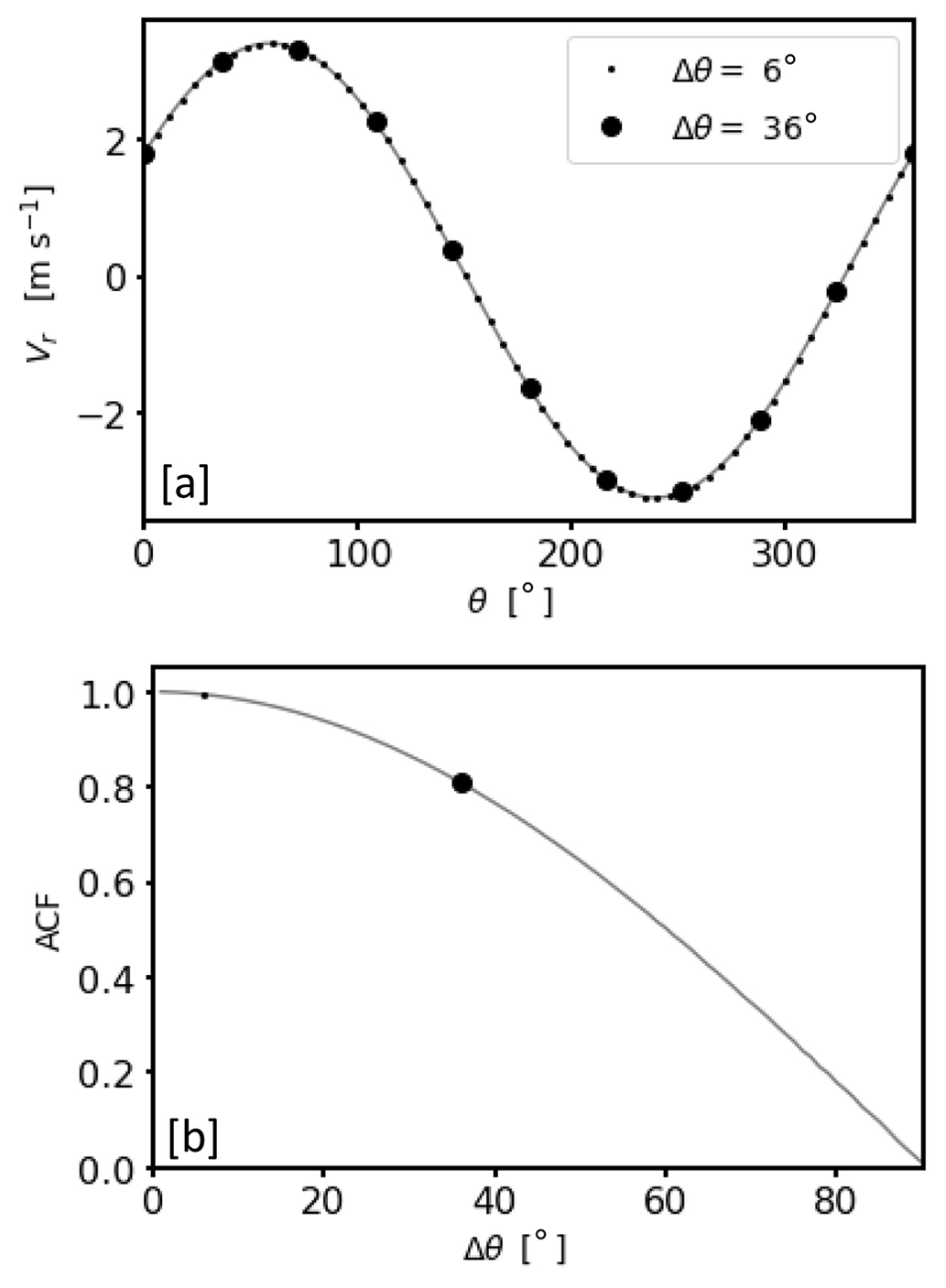
Figure B1 (a) Two theoretical examples for radial velocity measurements V_r from a conically scanning Doppler lidar with different azimuthal resolution, i.e., Δθ=6° and Δθ=36°. Gray background indicates the corresponding continuously resolved sine curve. (b) Normalized lag k=Δθ autocorrelation values of the continuous sine shown in (a) for azimuth steps between Δθ=1° and Δθ=90°. The dots indicate the maximum expected value of the autocorrelation function ACF (n=1; Δθ) = ACF_max between neighboring azimuthal measurement points for the discrete measurement series of different azimuthal resolution Δθ shown in (a).​​​​​​​

Appendix C: Intercomparison of background noise distribution between different StreamLine and StreamLine XR Doppler lidar systems

Background noise characteristics are best analyzed based on DL measurements at high altitudes where atmospheric signals are unlikely due to low aerosol density. DL measurements from three different StreamLine DL systems (DL78, DL172, DL177) at 1729 m height and from four different StreamLine XR DL systems (DL44, DL146, DL143, DL161) at 1737 m height are shown in Figs. C1 and C2, respectively. Note that the differences in the vertical height between the two types of DL systems are due to the different DL range gate lengths (i.e., 30 m for the StreamLine DL and 48 m for the StreamLine XR DL). The measurements represent the same measurement period, i.e., 29 July 2021 between 02:40 and 03:10 UTC. At the time of the measurement, all seven Doppler lidar systems were positioned next to each other at the GM Falkenberg site and were operated with the same configuration (see Sect. 2.1). Type B noise (i.e., high density of bad estimates around zero; see Sect. 2.2) characteristics are very pronounced in all three StreamLine DL systems (Fig. C1a–c). In the measurements with the StreamLine XR DL systems, type B noise is weak to moderate (Fig. C2a–d). None of the DL systems really show pure white noise characteristics (Figs. C1a2–c2 and C2a2–d2), i.e., uniformly distributed radial velocity estimates. Note that the measurement example for the DL161 is the only system that still has some signal at 1737 m height (Fig. C2d), although the measurements for all systems took place under the same atmospheric conditions.

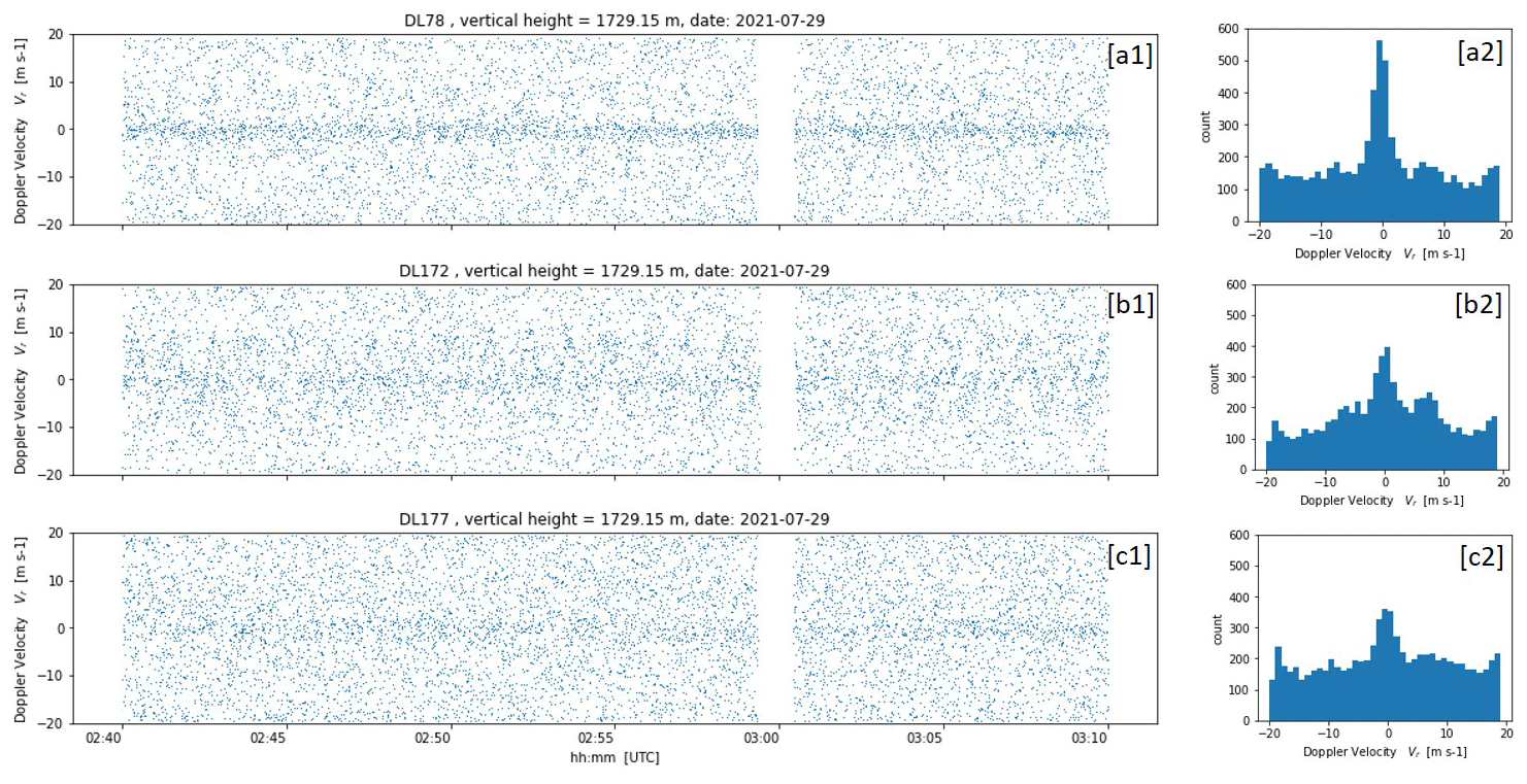
Figure C1 Measurements from three different Doppler lidar StreamLine systems at 1729 m height. Panels (a1)–(c1) show radial velocity time series plots from measurements with DL78, DL172, and DL 177 over a time interval of about 30 min. Panels (a2)–(c2) represent the associated radial velocity distributions.​​​​​​​

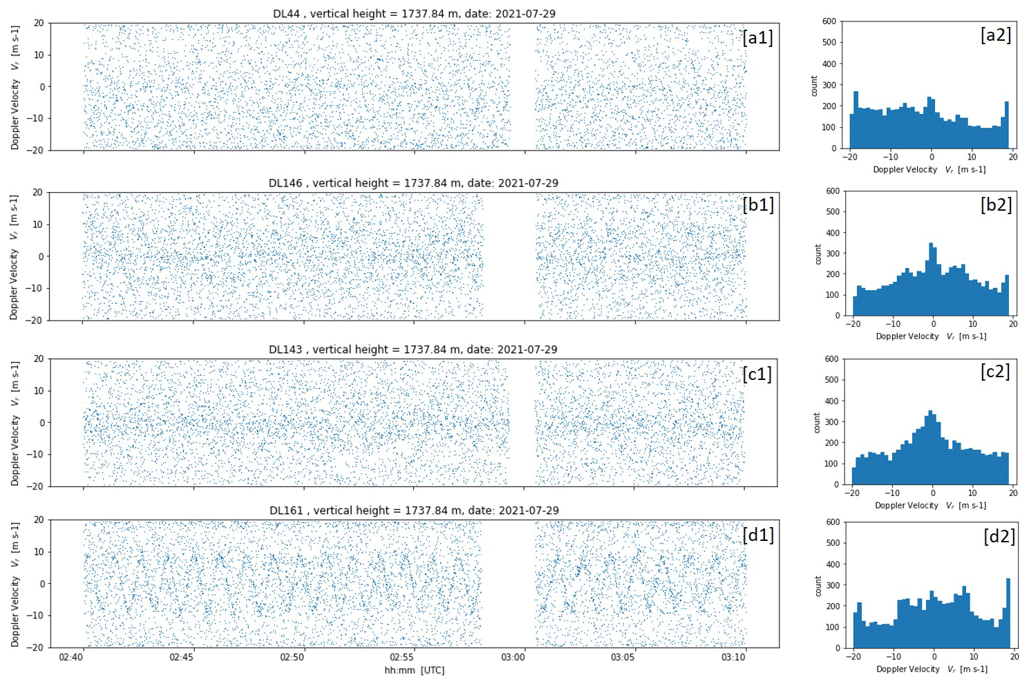
Figure C2 Measurements from four different Doppler lidar StreamLine XR systems at 1737 m height. Panels (a1)–(d1) show radial velocity time series plots from measurements with DL44, DL146, DL143, and DL177 over a time interval of about 30 min. Panels (a2)–(d2) represent the associated radial velocity distributions.​​​​​​​

Appendix D: Radial velocity uncertainty estimates

An equation for uncertainty estimates of DL radial velocity is given in Pearson et al. (2009) and reads

$$\begin{array}{}\text{(D1)}& \mathit{\sigma }\left(\mathrm{m}{\mathrm{s}}^{-\mathrm{1}}\right)=\mathrm{2}{\left({\mathit{\pi }}^{\mathrm{0.5}}/\mathit{\alpha }\right)}^{\mathrm{0.5}}(\mathrm{1}+\mathrm{0.16}\mathit{\alpha })\left(\mathrm{\Delta }\mathit{\nu }/N_{\mathrm{p}}^{\mathrm{0.5}}\right),\end{array}$$

with

$$\begin{array}{}\text{(D2)}& {\displaystyle }\mathit{\alpha }=\mathrm{SNR}/\left[\left(\mathrm{2}\mathit{\pi }{)}^{\mathrm{0.5}}\right(\mathrm{\Delta }\mathit{\nu }/B)\right],\text{(D3)}& {\displaystyle }{N}_{\mathrm{p}}=M{N}_{\mathrm{a}}\left(\mathrm{SNR}\right).\end{array}$$

Here, the system parameters N_p,B, and M denote the accumulated photocount, the bandwidth used, and the gate length in points, respectively. The signal spectral width Δν depends on both instrumental and atmospheric conditions (Doviak and Zrnic, 1993), i.e.,

$$\begin{array}{}\text{(D4)}& \mathrm{\Delta }\mathit{\nu }={\mathit{\sigma }}_{\mathrm{tot}}=\sqrt{({\mathit{\sigma }}_i{)}^{\mathrm{2}}+({\mathit{\sigma }}_a{)}^{\mathrm{2}}},\end{array}$$

with σ_i given through (please see Eqs. 6 and 7 in Frehlich, 2004)

$$\begin{array}{}\text{(D5)}& {\displaystyle }{\mathit{\sigma }}_i=\mathit{\lambda }\mathit{\omega }/\mathrm{2},\text{(D6)}& {\displaystyle }\mathit{\omega }={\displaystyle \frac{(\ln \mathrm{2}/\mathrm{2}{)}^{\mathrm{1}/\mathrm{2}}}{\mathit{\pi }\mathrm{\Delta }t}}={\displaystyle \frac{\mathrm{0.1873906}}{\mathrm{\Delta }t}},\end{array}$$

where λ denotes the wavelength of the Doppler lidar. Here, Δt denotes the pulse width which is used to calculate the spectral width ω and which can be transformed into a spectral width σ_i in velocity space via Eq. (D5). Note that in Pearson et al. (2009) not the pulse width Δt but the pulse length Δr is given as a lidar parameter. With knowledge of Δr the pulse width Δt can be calculated via

$$\begin{array}{}\text{(D7)}& \mathrm{\Delta }r=c\mathrm{\Delta }t/\mathrm{2},\end{array}$$

where c denotes the speed of light (Frehlich, 2004). The value σ_a in Eq. (D4) denotes the atmospheric broadening factor. In Pearson et al. (2009) it is assumed that σ_a=1 m s⁻¹.

Appendix E: On the determination of the critical radius r_c

Using the framework of the VV90D perspective, the critical radius r_c can be determined by analyzing DL measurements from higher range gate numbers where only background noise and no true signal characterizes the DL measurements. An example for such a situation is shown in Fig. E1. Here the circular rings with central radii r_i below r_c=4.5 show an increased availability of data which can be clearly assigned to “noise around zero”. For r_i>r_c the data availability is almost uniformly distributed. We know from our experience of working with various DL systems that the noise characteristics can be different. For that reason the above-described features are characteristic for the DL used in our studies and cannot be generalized.

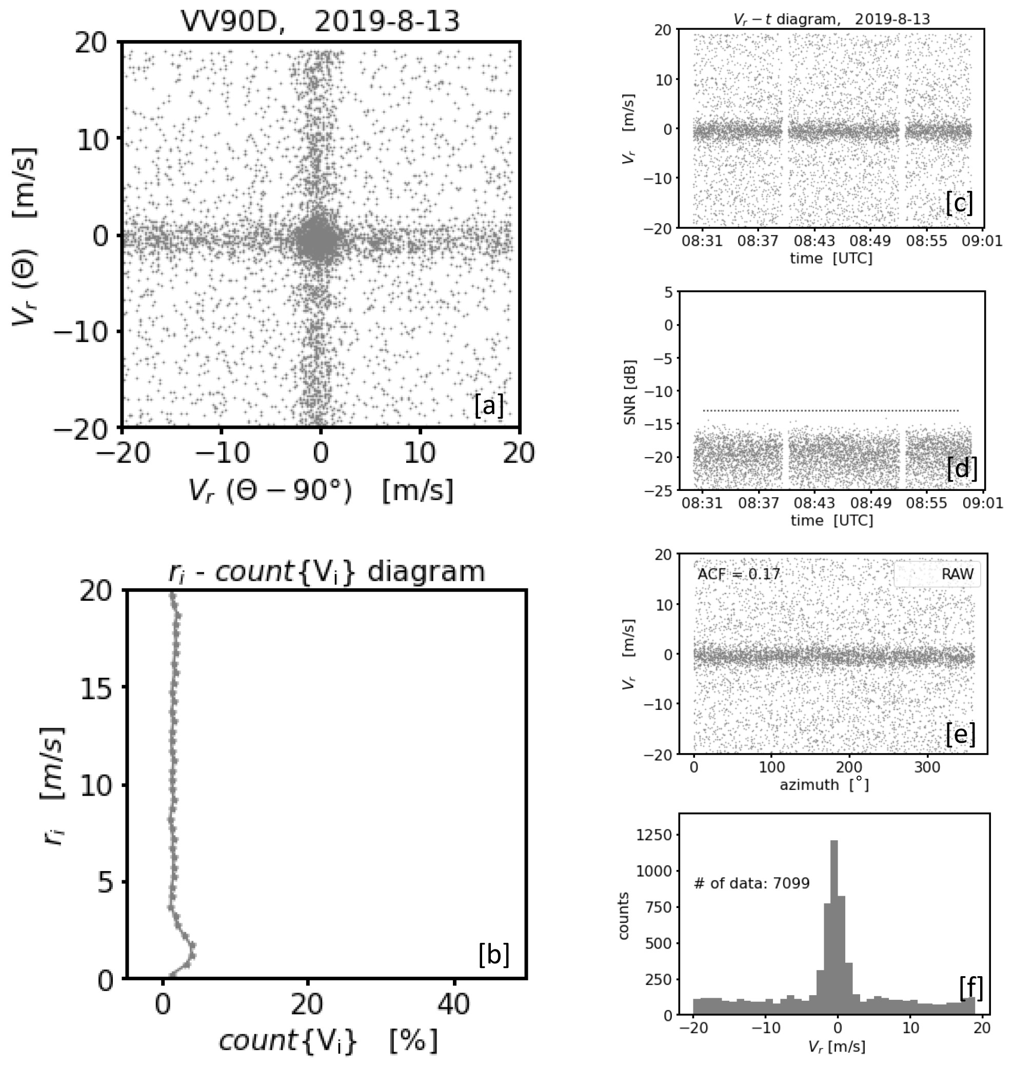
Figure E1 Noise characteristics of the Doppler lidar DL78. The data represent a 30 min time interval at range gate number 90. The panels on the left show (a) the VV90D perspective of the radial velocity measurements and (b) the corresponding r_i−count{V_i} diagram to describe the availability of data in different circular rings $r_i-\mathrm{\Delta }r\le r_i\le r_i+\mathrm{\Delta }r$ spanning the (V90,V) plane where $i=\mathrm{1},\mathrm{\dots },n$ with n∈ℕ and Δr=0.5 m s⁻¹. The panels on the right are with regard to their order analogous to the plots shown in Fig. 1, i.e., (c) the time series plot of the DL radial velocity estimates, (d) the corresponding time series plot of the signal-to-noise ratio (SNR), (e) the corresponding VAD plot of the measurements, and (f) the histogram of DL radial velocity estimates.​​​​​​​

Appendix F: Guidance on a practical implementation of coarse filter II

From a practical point of view there are four further issues which are worth pointing out for DL users when applying coarse filter II. Firstly, from our experience we know that for an azimuthal resolution of Δθ=1° a value of ACF$(\mathit{\tau }=\mathrm{1})<\mathrm{0.95}$ indicates a relatively high fraction of bad estimates (see also the examples shown in Fig. 1). Hence for a successful application of the method the threshold value ACF_thresh = 0.95 is recommended. For DL measurements with azimuthal resolution lower than Δθ=1° this value can be different (see Sect. B). Secondly, it can be useful to apply coarse filter II a second time for a further improvement of the filter results. Prior to a second application, however, the diagrams representing the VV90D perspective have to be re-drawn based on the filtered time series obtained from the first application of coarse filter II but with a phase shift in the opposite direction, i.e., $\mathrm{\Delta }\mathrm{\Theta }=+\mathrm{90}$°. The outcome of a second application of coarse filter II (indicated by capital letter B in the plot legends) in comparison to the results obtained from the first application (indicated by capital letter A in the plot legends) is shown in Figs. 9 and 10. In these cases, however, the second application (i.e., coarse filter II – B) has no significant advantage compared to the first application (i.e., coarse filter II – A) since the ACF values for each iteration step (see Fig. 9c, d) remain above the ACF threshold value. Hence, there is no need to discard subsets V_i from the circular rings $r_i-\mathrm{\Delta }r\le r_i\le r_i+\mathrm{\Delta }r$ under consideration. Note, however, that although no data have been discarded the final filter results after the second application (see Fig. 10) show a reduced data availability in comparison to the first application. This effect is a rather technical consequence of the opposite shift of the filtered time series obtained based on the first application. Thirdly, there are also practical limits in the application of coarse filter II. They arise when for the initial circular ring with a maximum number of data the value of the data count is already very low. This is especially the case when the original time series is highly contaminated with noise. In this case the gaps due to flag values of the initially determined time series are too large so that no meaningful results are obtained with a linear interpolation to fill these gaps. Accordingly, the corresponding ACF value of the time series is not suitable to be used as a trustworthy indicator for the occurrence of bad estimates. Since it is difficult to give a threshold value for the required frequency maximum to exceed in order to get reliable ACF results, it is recommended to always check the ACF of the finally filtered time series and to use only those filtered series where the condition ACF > ACF_thresh is met. Fourth, in the case of pronounced type B noise it may happen that the data availability in circular rings including most of noise around zero is comparable to the availability of data in rings including most of the true signals, i.e., good estimates (see Fig. 7e). The challenge in such a case is to ensure that for the generation of the initial filtered time series the circular ring $r_i-\mathrm{\Delta }r\le r_i\le r_i+\mathrm{\Delta }r$ with MAX(count{V_i}) has been chosen correctly, i.e., the subset of high data availability with the good signals instead of the bad signals. To achieve this it may be helpful to always test the data availability distribution per circular ring (i.e., the distribution displayed in the r_i−count{V_i} diagram) on multi-modality. When multi-modality occurs and a circular ring with a central radius r_i<r_c representing a local maximum of data does exist, all circular rings with central radii r_i<r_c should be excluded prior to employing coarse filter II. Here, r_c denotes a critical radius below which one has to expect a pronounced concentration of bad estimates if the noise is of type B. How this value can be determined is described in more detail in Appendix E. For the DL used in our studies we found r_c =  4.5. This value is also relatively constant with time and explains the missing data in the r_i−count{V_i} diagram shown in Fig. 9e for r_i<4.5 compared to the r_i−count{V_i} diagram shown in Fig. 7e for the same measurement interval. It should be noted, however, that the above-described procedure of circular ring exclusion is not recommended for type-B-contaminated measurements during weak and stationary wind conditions. In such a case multi-modality in the r_i−count{V_i} diagram is not expected either; since with decreasing wind speeds circular rings including most of the true signals and circular rings including most of the noise around zero increasingly merge, it carries the risk of discarding a huge fraction of good estimates. The latter would negatively affect the possibility to derive reliable wind and turbulence values during weak wind conditions.

Appendix G: Strategy for implementation of approach I and approach II

The systematic intercomparison of both filtering techniques in Sect. 4.4 leads to the following general conclusion: for filter approach I the most limiting factor is noise around zero (type B noise), while problems may arise for filter approach II due to nonstationarity in the wind field. These limiting factors are very different in nature. For approach I the limitations are due to issues with the DL system's background noise. This seems to be an instrumental issue and there might be a chance to get this problem solved by the manufacturer. In contrast, the limitation of approach II is that it cannot be used for all wind situations. The DL end user has no influence on this and would therefore have to accept these limitations when using the filter approach. Hence, from our point of view there are two options for an implementation of the filtering techniques into an operational product retrieval process. Provided that the DL's background noise is always of type A, an implementation of approach I appears to be sufficient to detect and reject bad estimates. If the DL system's background noise varies between type A and type B noise both filtering techniques should be implemented. This should be combined with a decision strategy that ensures the employment of approach I in the case of measurements contaminated with type A (or no) noise or the employment of approach II in the case of type B noise. In order to be able to choose between the two options a good understanding of the measurement systems' noise characteristics is required.

The combined application of both approaches presents another challenge for the implementation process. From a visual perspective on the measurement data it is easy to differentiate between type A and type B noise. However, for a routine processing an automated decision-making strategy would be required. This could be arranged as follows: first one could apply both filter approaches for each measurement interval under consideration. In doing so one obtains for each measurement interval two differently filtered datasets which do not necessarily have to be the same. If one knows the good radial velocities, one also knows the bad ones at the same time. Hence, with correct filtering the distributions of the bad estimates can provide useful information about the type of noise occurring over the measurement interval. In the case of type A noise one would expect uniformly distributed data, whereas in the case of type B noise a maximum close to zero would be characteristic (see also Sect. 2.2). Eventually, on this basis a decision on the appropriate filter method would be possible.

Appendix H: TKE from noise-free DL measurements

For DL measurements without noise issues (Fig. H1, 1), reasonable TKE products based on the turbulence retrieval method outlined in Smalikho and Banakh (2017) can be obtained (Fig. H2). The method relies on a work by Kropfli (1986) where the focus was on the determination of TKE from radar measurements. When transferring the approach to DL measurements, Smalikho and Banakh (2017) suggest additional correction terms for both the underestimation of TKE due to pulse volume averaging effects (${\mathit{\sigma }}_{\mathrm{t}}^{\mathrm{2}}$) and an overestimation due to the instrumental error of the radial velocity estimation (${\mathit{\sigma }}_{\mathrm{e}}^{\mathrm{2}}$). A comparison of DL-based TKE measurements with independent sonic measurements at a measurement height of 90 m is shown in Fig. H2. To clarify the effect of the ${\mathit{\sigma }}_{\mathrm{t}}^{\mathrm{2}}$ and ${\mathit{\sigma }}_{\mathrm{e}}^{\mathrm{2}}$ corrections, TKE values without (KR1986 hereafter) and with the suggested corrections (SM2017 hereafter) are shown. With the KR1986 retrieval the TKE underestimation due to the pulse averaging effect is most pronounced during night, i.e., while the atmospheric boundary layer is in a stable state. Under stable conditions, smaller-scale eddies primarily exist which obviously could not be fully resolved over the pulse volume. During the day the corrections are smaller because the main fraction of the observed TKE was associated with larger and thus resolvable eddies. Although with SM2017 values of TKE are overestimated on average by 6.3 %, the results are in better agreement with sonic data than the KR1986 values which underestimate the TKE by −12.45 % on average. Therewith the finally corrected TKE is in good agreement with the sonic TKE, which gives evidence for a proper functioning of the retrieval method itself.

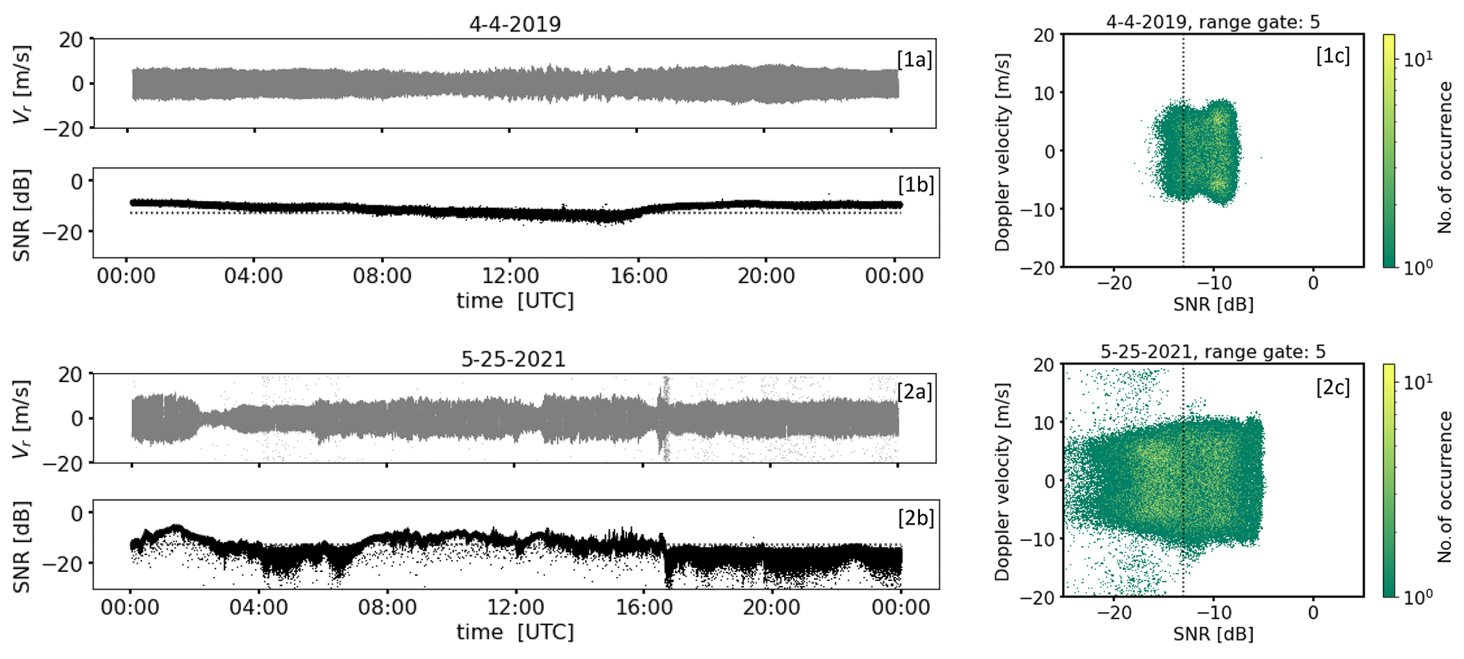
Figure H1 Time series plots of Doppler lidar radial velocity V_r (1a, 2a) and corresponding SNR values (1b, 2b) from a conically scanning Doppler lidar for one day, i.e., 4 April 2019, with good measurement conditions which are reflected in relatively high SNR values and another day, i.e., 25 May 2021, with unfavorable measurement conditions which are reflected in relatively low SNR values. The corresponding (V_r, SNR) plots are shown in panels (1c) and (2c). The dotted lines in panels (1b), (1c), (2b), and (2c) indicate the SNR threshold value SNR_thresh = −12.7 dB.

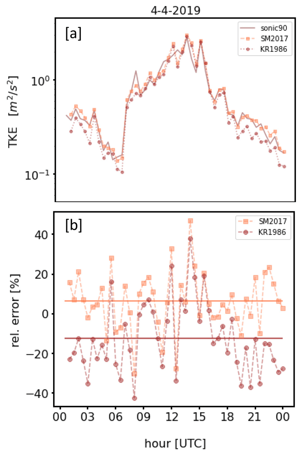
Figure H2 (a) Time series of TKE at 90 m height derived from sonic anemometer measurements and from DL data using the methods proposed by Kropfli (1986) (KR1986) and Smalikho and Banakh (2017) (SM2017), respectively, for 4 April 2019. (b) Relative error between Doppler lidar TKE and sonic TKE for the sample day shown in (a). The horizontal lines indicate the corresponding mean relative error over the whole day.