Performance evaluation of MeteoTracker mobile sensor for outdoor applications

The morphological complexity of urban environments results in a high spatial and temporal variability of the urban microclimate. The consequent demand for high-resolution atmospheric data remains a challenge for atmospheric research and operational application. The recent widespread availability and increasing adoption of low-cost mobile sensing offer the opportunity to integrate observations from conventional monitoring networks with microclimatic and air pollution data at a finer spatial and temporal scale. So far, the relatively low quality of the measurements and outdoor performance compared to conventional instrumentation has discouraged the full deployment of mobile sensors for routine monitoring. The present study addresses the performance of a commercial mobile sensor, the MeteoTracker (IoTopon Srl), recently launched on the market to quantify the microclimatic characteristics of the outdoor environment. The sensor follows the philosophy of the Internet of Things technology, being low cost, having an automatic data flow via personal smartphones and online data sharing, supporting user-friendly software, and having the potential to be deployed in large quantities. In this paper, the outdoor performance is evaluated through tests aimed at quantifying (i) the intra-sensor variability under similar atmospheric conditions and (ii) the outdoor accuracy compared to a reference weather station under sub-optimal (in a fixed location) and optimal (mobile) sensor usage. Data-driven corrections are developed and successfully applied to improve the MeteoTracker data quality. In particular, a recursive method for the simultaneous improvement of relative humidity, dew point, and humidex index proves to be crucial for increasing the data quality. The results mark an intra-sensor variability of approximately ± 0.5 °C for air temperature and ± 1.2 % for the corrected relative humidity, both of which are within the declared sensor accuracy. The sensor captures the same atmospheric variability as the reference sensor during both fixed and mobile tests, showing positive biases (overestimation) for both variables. Through the mobile test, the outdoor accuracy is observed to be between ± 0.3 to ± 0.5 °C for air temperature and between ± 3 % and ± 5 % for the relative humidity, ranking the MeteoTracker in the real accuracy range of similar commercial sensors from the literature and making it a valid solution for atmospheric monitoring.

1 Introduction

The coverage of the Earth's surface by atmospheric monitoring networks remains challenging, especially in remote locations, poor countries, and complex terrain. Within the last category, the urban environment requires long-term monitoring at high spatial and temporal resolutions as turbulence structures play a key role in inertial and thermal ventilation (Barbano et al., 2020; Cintolesi et al., 2021). To fill the gap, classical urban observational networks are supported by spot-on intensive field campaigns for intra-urban flow detailing and turbulence analysis. The recent development of low-cost sensors provides a novel opportunity to integrate the existing monitoring networks with cheaper yet reliable solutions. Nowadays, monitoring protocols for fixed low-cost weather stations have adopted crowdsourcing approaches (Meier et al., 2017; Fenner et al., 2021) to increase the spatial coverage of urban areas, with the creation of community networks (Jiao et al., 2016) for environmental monitoring. Contextually, the adoption of mobile sensors and smartphones is increasing, carrying the typical shortcomings of novel approaches, such as the lack of protocols for mobile sensing, outdoor accuracy, and long-term reliability. Data quality from mobile sensing will require suitable but transferable sensor calibration strategies (Xu et al., 2019; deSouza et al., 2022), as well as the development of accurate correction algorithms (Huang et al., 2023). The development of dedicated platforms (e.g. den Ouden et al., 2021) provides a virtual environment where quality-controlled mobile data can be safely stored and shared.

Two major classes of sensors have been developed according to their application scopes, i.e. the study of microclimate and air quality. As a short note, air quality sensors mostly monitor regulated pollutants, such as particulates, nitrogen dioxide and ozone, and/or greenhouse gases such as carbon dioxide (e.g. Johnson et al., 2016; Van den Bossche et al., 2016; Puri et al., 2020; Gómez-Suárez et al., 2022; Ganji et al., 2023). Microclimate sensors are firstly designed for monitoring the urban thermal environment (Kousis et al., 2022), but the radiative properties of the atmosphere (Heusinkveld et al., 2023), evapotranspiration (Markwitz and Siebicke, 2019), and wind-related quantities (Droste et al., 2020) have also found recent interest. A key ensemble of this second category consists of mobile sensors suitable for measuring the thermo-hygrometric characteristics of the atmosphere on the move. The sensor suite is typically composed of a thermo-hygrometer or a thermo-logger, but examples of complete weather stations mounted on moving vehicles (Heusinkveld et al., 2014; Emery et al., 2021) or integration with automatic infrared cameras (Lindberg, 2007; Acosta et al., 2022) are also documented. Two main categories of sensors are also used: research-grade instrumentation designed for conventional weather stations and adapted for mobile use and low-cost mobile sensors. In addition, mobile sensing using smartphones is also accessed nowadays thanks to the presence of temperature sensors that are oftentimes installed within some devices (e.g. Cabrera et al., 2021) or the use of alternative data proxies such as the temperature of the smartphone battery (Overeem et al., 2013; Droste et al., 2017), along with the potential crowdsourcing from large communities. Oftentimes, the sensor fabric is modified, adding homemade radiation shields (Sun et al., 2009; Leconte et al., 2015) and ventilation pipes (Tsin et al., 2016). Despite walking being an explored option in the literature, the vast majority of mobile monitoring is performed using bicycles or motor vehicles. This allows a wide spatial coverage of the urban and surrounding areas (Sun et al., 2019); a large number of monitoring scans (Emery et al., 2021); a long-term assessment (Charabi and Bakhit, 2011); and a variety of monitoring techniques, including spot-on measurements (Qaid et al., 2016) and transect inspections (Unger et al., 2001).

The top-trend research topic is the urban heat island (UHI) effect, where mobile sensing offers a denser representation of the canyon-level air temperature (Stewart, 2011) inside the urban context. Intra-urban UHI and local thermal effects are attributed to the land cover, urban morphology, and aspect ratio of the urban canyons. Yan et al. (2014) used an instrumented bicycle to infer the magnitude and spatial characteristics of the air temperature variations related to the landscape parameters characterizing the immediate environment of the measurement sites. Focusing on the street canyon, Sun (2011) conducted a mobile survey by bike to show a positive correlation between the air temperature and the height-to-width ratio of the canyon, green-area coverage, and building ratio. Covering a larger spatial area by instrumented car, Noro et al. (2015) observed consistent temperature differences in the range of 0.5 to 2.5 °C, depending on the local climate zone (LCZ, Stewart and Oke, 2012) passed through. Shi et al. (2018) confirmed the applicability of mobile sensors in assessing the thermal properties within high-density heterogeneous urban contexts, evaluating an intra-LCZ air temperature difference up to 2 °C within six diverse LCZs. In agreement with traditional studies on the local-scale UHI effect (e.g. Di Sabatino et al., 2020), these studies support strategies that increase vegetation coverage at the expense of buildings to mitigate urban warming and to create a comfortable thermal environment. Other uses of mobile sensing include the assessment of the impacts of the urban morphology on the cooling effect of small rivers (Park et al., 2019) and the influence of external factors on the temperature field within the urban context (Rajkovich and Larsen, 2016). The temperature maps obtained through mobile sensing are also suitable for validating numerical simulations (Hsieh et al., 2016) and for application to thermal comfort and local climate stress (Koopmans et al., 2020).

The advantage of a mobile sensor is the large spatial coverage ensured by continuous monitoring while moving, which can be performed actively through ad hoc experiments or passively during daily life activities. As a drawback, measurements will be dependent on both time and space, revealing non-trivialness to assess phenomena such as the UHI effect. Schwarz et al. (2012) introduced a correction for decreasing temperatures due to progressing time so that they would not confound air temperature differences due to changing surroundings with temperature differences because of evening cooling. To compensate for the different time responses of the mobile sensor related to the reference, namely the thermal inertia error, Qi et al. (2022) introduced an initial temperature correction. In previous research, the response time of mobile sensors was determined by cycling through a tunnel (Brandsma and Wolters, 2012) or by sensitivity tests comparing in situ and mobile measurements (Emery et al., 2021). To deal with the response time at the beginning of a monitoring session, we can use statistics to eliminate the time required by the sensor to adjust its internal temperature to the ambient air. Depending on the scope of the investigation, a temperature decline correction is needed to compensate for the background temperature evolution while completing the route (Brandsma and Wolters, 2012). Finally, mobile sensors need a protocol for outdoor validation before usage, which is missing in most applications from the literature. For low-cost sensors, this step is required owing to the discrepancy often observed between the ideal accuracy of the sensor (that acquired in the laboratory under controlled conditions) and the real one evaluated in the field. Establishing an outdoor protocol for low-cost sensors is mandatory to infer the reliability of their measurements and under which circumstances they perform at their best (Brattich et al., 2020). Similarly, research-grade instrumentation is mostly built for fixed-location monitoring, and a reliability test should be performed for mobile usage.

In this paper, we provide a quality assessment and performance evaluation of a recently developed commercial mobile sensor for monitoring the urban microclimate called MeteoTracker (MT), developed by IoTopon Srl. To the best of our knowledge, the MT was used in very few scientific research endeavours with promising results (Cecilia and Peng, 2022; Carraro, 2022). However, these evaluations focused only on the air temperature data of a single MT with respect to other low-cost mobile sensors, leaving gaps in the overall performance evaluation. In the current paper, we aim to provide a more robust and comprehensive assessment of the MT outdoor performance, which includes evaluating the intra-sensor variability of multiple MTs simultaneously operating under equal ambient conditions and validating the MT's measurements against a research-grade reference in both optimal (while moving) and non-optimal (as a fixed station) operational usage. This investigation also provides a set of exploitable methods to correct the MT measurements and enhance their outdoor accuracy, validated for different climate zones and seasons, and their sensor usage, customized for each measured variable of the MT. Ultimately, this analysis will evaluate the potential of the MT to be adopted as a research-grade sensor.

After this introduction, Sect. 2 introduces the MT sensor and data flow; Sect. 3 describes the multi-step procedure adopted in this paper to address the sensor performance, while Sect. 4 presents the results from each step. Section 5 contextualizes the MT performance in the context of mobile sensing. Section 6 presents the conclusions.

2 The MeteoTracker

2.1 The sensor

The MT is a low-cost portable weather station (see Fig. 1) that samples several meteorological variables while moving jointly with its carrying vehicle (mobile sensor). The device hardware comprises a compact case (75 mm × 75 mm × 35 mm) with a magnetic base to secure the station to the vehicle, tested at regulatory speed limits on highways. The case can also support the installation of a string to secure the station to a non-metal moving object. The aerodynamic shape supports the stability above the vehicle, while the extensive frontal and back overtures (air filters) enable a large air volume sampling and good internal ventilation. The sensing board is supplied by different capacitive–resistive sensors, measuring air temperature T, relative humidity RH, and atmospheric pressure P with a declared accuracy close to that of a research-grade instrument (see Table 1). In addition, the sensor measures the solar radiation intensity indicator R, but the accuracy and operational range are not provided by the manufacturer. Derived quantities are also automatically computed by the station using known empirical thermodynamic laws and formulas. Among those, the dew-point temperature T_d and the humidex index HDX (an index which estimates the anthropogenic well-being associated with climate; see Masterton and Richardson, 1979) are both obtained by combining air temperature and relative humidity in some capacities. For the dew point, Lawrence (2005) explored the intricacies and possible empirical, theoretical, and simplified expressions with the classical thermodynamics, while humidex is defined as

$$\begin{array}{}\text{(1)}& \mathrm{HDX}=T+\mathrm{0.5555}(e-\mathrm{10}),\end{array}$$

where e is the water vapour pressure in hPa, and T is in degrees Celsius. Altitude Z in metres above the mean sea level is also derived from the atmospheric pressure; with it, the vertical thermal gradient is computed (in °C (100 m)⁻¹).

The sensor is not shielded from solar radiation. Still, it is supplied with a radiation error correction system (RECS), a patent of the manufacturer to correct the effect of solar radiation on temperature while the sensor is moving at more than 7 km h⁻¹.

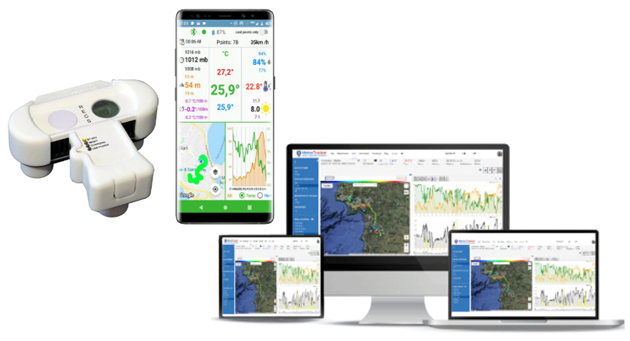
Figure 1 The MT and its components. Left to right: the mini-weather station, the mobile application, and the web platform. Collage from https://meteotracker.com/ (last access: July 2022).

The station has an internal memory that ensures up to 250 h of usage, and it is remotely controlled, using a customized application on the user's smartphone, through a one-to-one connection (one station is controlled by one application). Through the app, the user selects the sampling rate of the sensors in terms of both frequency (at least 1 Hz) and distance (at least 1 m), letting the device select and use the highest resolution according to the vehicle's speed. The user decides to enable or disable the sensor calibration at each start and stop of the vehicle and also decides on the temperature correction due to the sensor movement (whether the sensor usage is mobile or in a fixed location). The app uses the smartphone GPS to geolocate the station and to compute the initial altitude (see Sect. 3), and it provides the vehicle speed V_s.

Table 1 Significant variables measured by the MT, with accuracy and operational range according to the manufacturer.

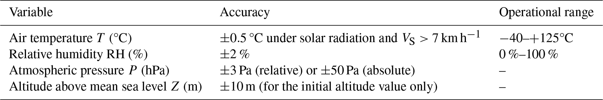
^∗ RECS, patent of the manufacturer.

On the app, the user can visualize the livestreaming of the monitoring session from a georeferenced map and the time series of the measured variables. At the end of each session, measurements are stored locally in the smartphone and uploaded on a dedicated online platform for visualization, data retrieval, download, and sharing with other users.

2.2 Data flow and visualization

The mobile app and smartphone connectivity regulate the flow of the data collected by the station. The station and mobile app have to remain connected via Bluetooth for the whole duration of the monitoring session to ensure the flow and storage of the measurement (as a choice of the manufacturer, the station itself does not have an internal memory). A stable GPS and internet connection are required to compute the altitude during the monitoring session, to livestream the monitoring session through the dedicated online dashboard, and to upload the data on the platform once over. The user can define the level of privacy (private, public, and public anonymously) of the collected data before initiating a monitoring session. Both public sessions will be streamed and data will be shared through the platform. Public data on the platform can be reached by other users through a dashboard, with the permission to visualize or download depending on the type of account bought alongside the device. An example of data visualization on the dashboard is shown in Fig. 2.

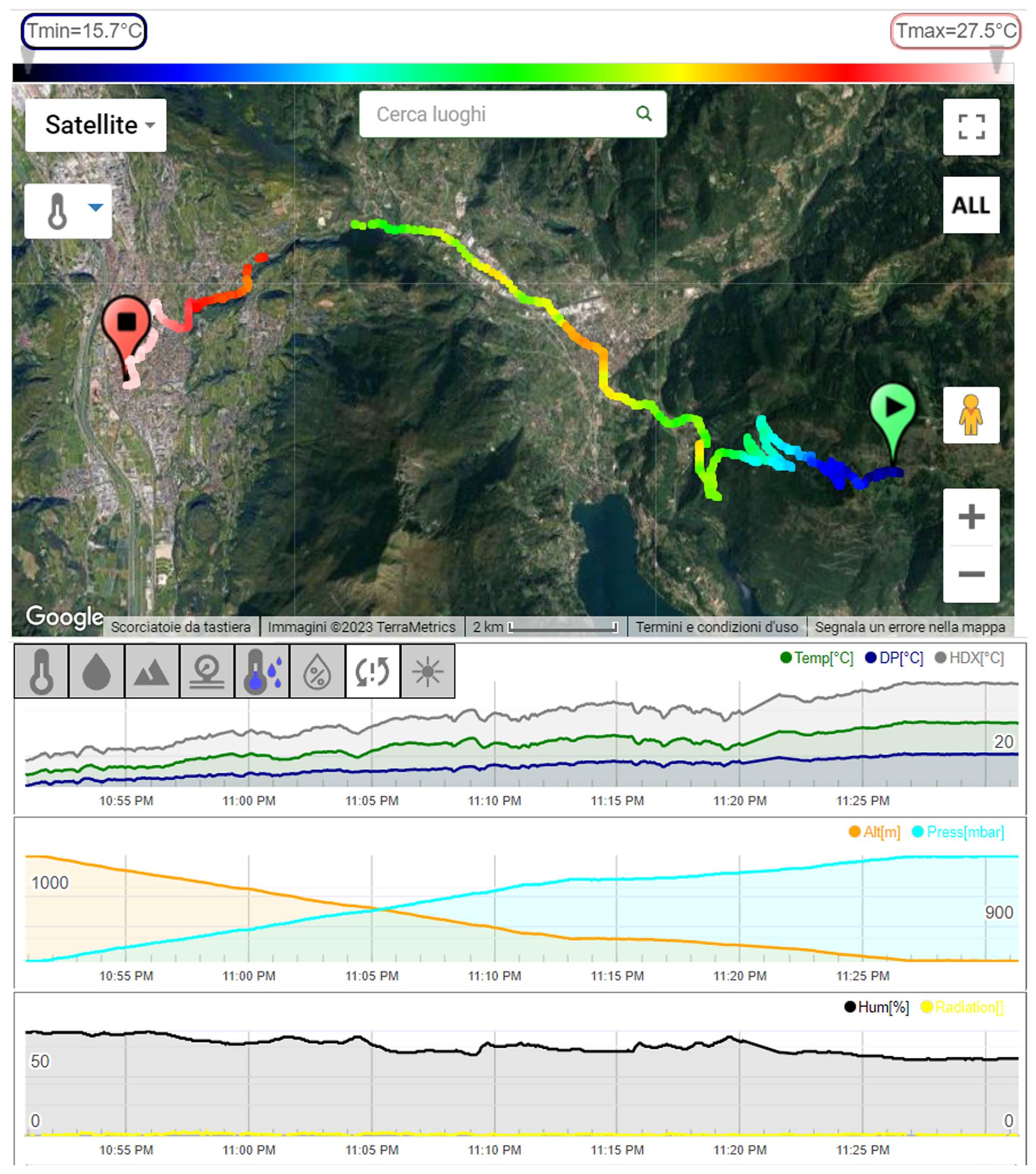
Figure 2 Example of MT track and collected data as visualized on the online dashboard. The coloured points on the map are the air temperature measured by the sensor. Graphs are the reconstructed time series of each measured and derived variable along the vehicle track. Source: https://app.meteotracker.com/ (last access: July 2022).

The MT track is superimposed on a Google map, showing the point-by-point georeferenced map of a measured variable (air temperature in the example of Fig. 2), giving a qualitative but effective intake of the collected measurements. The time series of the same variables can be displayed directly on the dashboard for a more quantitative disposal of the data.

The price of the device with full permission on the platform in 2021 was EUR 119 (including taxes); the recent updates (2023), the new connectivity tools, and the set of additional accessories have raised the costs of this sensor, which remains below EUR 400.

2.2.1 A brief note on data storage

As previously described, the MT is not supplied with an internal memory; therefore, data collected during the monitoring sessions flow directly into the smartphone application via Bluetooth and are stored in the smartphone's internal memory. The limitation to data storage is only due to the available internal memory of the smartphone connected to the MT. Limiting these considerations to the experience gathered during the monitoring activities described within this paper, the amount of memory necessary for running an MT monitoring session is small: the smartphone application takes 53.1 MB of space, and each data point collected within a monitoring session is less than 2 KB. As a practical example, a monitoring session of 500 km at the finer resolution generates fewer than 17 MB of data. Once the monitoring session is ended and the data are uploaded on the platform, data stored on the smartphone can be deleted, saving internal memory.

3 Reliability assessment: a multi-step validation process

The validation process of MT measurements is performed in four steps: (i) identification and removal of the period of adjustment to the environmental conditions, (ii) evaluation of the intra-sensor variability under similar operational conditions, (iii) confrontation with a reference station in fixed-location mode, and (iv) confrontation with a reference station on the move. Three different cities hosted one or more steps of this assessment, namely Bologna (steps i and ii) and Savona (step iii) in Italy and Wageningen (iv) in the Netherlands. This choice ensures the testing of the sensors in different climate areas, classified following the Köppen–Geiger climate classification (Beck et al., 2018) as humid subtropical climate (Cfa), hot summer Mediterranean climate (Csa), and temperate ocean climate or subtropical highland climate (Cfb), respectively, for Bologna, Savona, and Wageningen¹. Each step is a key element to assess the self-consistency of the instrumentation and to evaluate its use for research purposes. The process evaluates the strengths and weaknesses of the MT, allowing us to expose the reliability limit of this specific low-cost sensor but also enabling the study and computation of possible post-processing solutions to improve the data quality and usability.

3.1 Outlier removal and identification of the adjustment period

As a fundamental step in data post-processing, the literature has proposed several methods to identify and remove outliers from a dataset. Typical methods are based on the a priori assumption that the dataset can be divided into subperiods wherein the measurements are distributed following a known function (typically a Gaussian distribution). A well-known example of these methods is given by Vickers and Mahrt (1997), where the outlier is defined as a value larger than 3.5 standard deviations from the mean in a certain time interval. Using this method over 30 min windows, Barbano et al. (2021) obtained a reliable cleaning performance for fast-sampling meteorological data within the urban canopy. Working with low-cost sensors for air quality and thermal comfort detection, Brattich et al. (2020) applied the Hampel filter (Hampel, 1974) to 1 min data to detect values beyond 2 median absolute deviations over 7 min windows and to replace them with the median over the same interval.

The aforementioned methods are tuned on traditional measurement techniques, where instruments sample meteorological or air quality data for a “long” period and at a fixed location. We can infer that monitoring sessions with MTs will be very short in time (as long as the vehicle travels) and frequent, not providing a sufficient amount of data to make a priori assumptions on their distribution. Moreover, we can assume that, after each monitoring session, the user would unmount the MT from the vehicle and bring it into an indoor environment for security reasons. At the onset of the next session, the MT will likely need a certain amount of time to adjust to the change of location, i.e. a change in the ambient temperature and relative humidity. The inter-quartile range (IQR) outliers' removal method (Hubert and Van der Veeken, 2008) serves the purpose of removing both the outliers and the initial adjustment period. This method applies to the entire sample, and it is not based on any assumption about the data distribution. It is based on the definition of upper and lower limits beyond which values are classified as outliers. Specifically, any data point x is an outlier if

$$\begin{array}{}\text{(2)}& \begin{array}{rl}& x<Q_{\mathrm{1}}-\mathrm{1.5}\mathrm{IQR},\\ & x>Q_{\mathrm{3}}+\mathrm{1.5}\mathrm{IQR},\end{array}\end{array}$$

where Q₁ and Q₃ are the first and third quartiles, respectively, and IQR=Q₃–Q₁. When needed, the IQR method is pre-empted by a linear detrending. The outliers identified at the beginning of the session mark the adjustment period and are just removed. Outliers given by spikes within the session are instead replaced with the median of the data distribution.

3.2 Intra-sensor variability

Low-cost sensors have proven to be reliable and accurate under laboratory conditions, yet they show larger inconsistencies when used outdoors under real-world atmospheric conditions. This is due to the fast transitions and heterogeneity of the atmospheric conditions compared to the rather constant and homogeneous laboratory flow. The response of low-cost sensors to the natural oscillations of the atmospheric variables can cause discrepancies between sensors' measurements due to the different sensor responses. The intra-sensor variability test is an open-air experiment, where multiple sensors operate under the same environmental conditions to infer the consistency among different sensors.

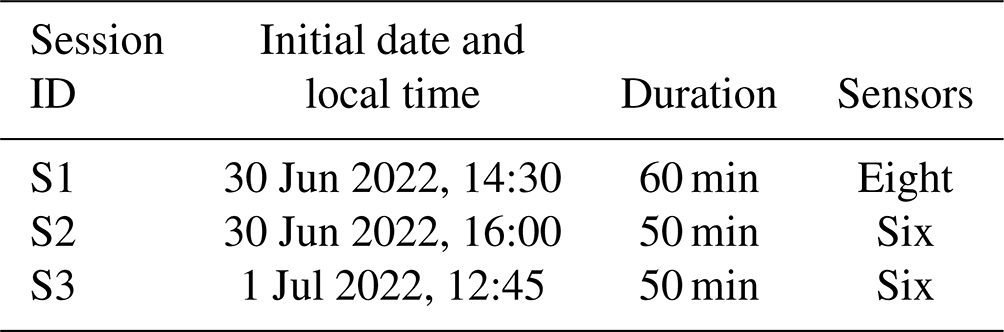
With regard to the scope, three monitoring sessions were designed to operate multiple MTs simultaneously (in groups of six, six, and eight MTs for practical reasons). During each session, the MTs within each group were mounted on top of a designated electric car and controlled by an equal number of smartphones by the passenger. The MTs were placed side by side in the front part of the car's top, as close as possible to the car axis to avoid capturing flows from lateral edges. The location on the car top minimizes the sensor's exposition to the direct heat sources of the car (engine, brakes, wheels) while maximizing the exposition to the fresh air that has not interacted with the car before being sampled by the sensor. MTs were aligned perpendicularly to the car axis along a single line: this prevents mutual shielding and exposes each MT directly to the flow. The spacing between MTs was approximately twice the lateral dimension of a single MT. A 50–60 min drive around the city centre and outskirts is then performed during each session, starting and ending at the Department of Physics and Astronomy of the University of Bologna (44°29^′57.1^′′ N, 11°21^′13.8^′′ E) and passing through different neighbourhoods and local ambient conditions to capture most of the morphology variability of the city. Table 2 summarizes the general information on the sessions.

Table 2 Overview of the intra-sensor variability tests

The three sessions were analysed independently due to the change in the environmental conditions, the starts and stops that occurred during the drive, and the slightly different trajectories adopted. Thus, we adopted a first session to tailor our post-processing schema to the measurements while testing those on the remaining sessions.

3.3 Fixed-location comparison

The reliability and trustworthiness of low-cost sensors are typically at stake when used outdoors as large and sharp transitions in the environmental conditions (sudden temperature drops, wind gusts, etc.), as well as extreme regimes (saturation, rain, and snowfall, etc.), are often demanding for sensor accuracy. For these reasons, a comparison with research-grade instrumentation is convenient to test the actual accuracy of low-cost sensors outdoors.

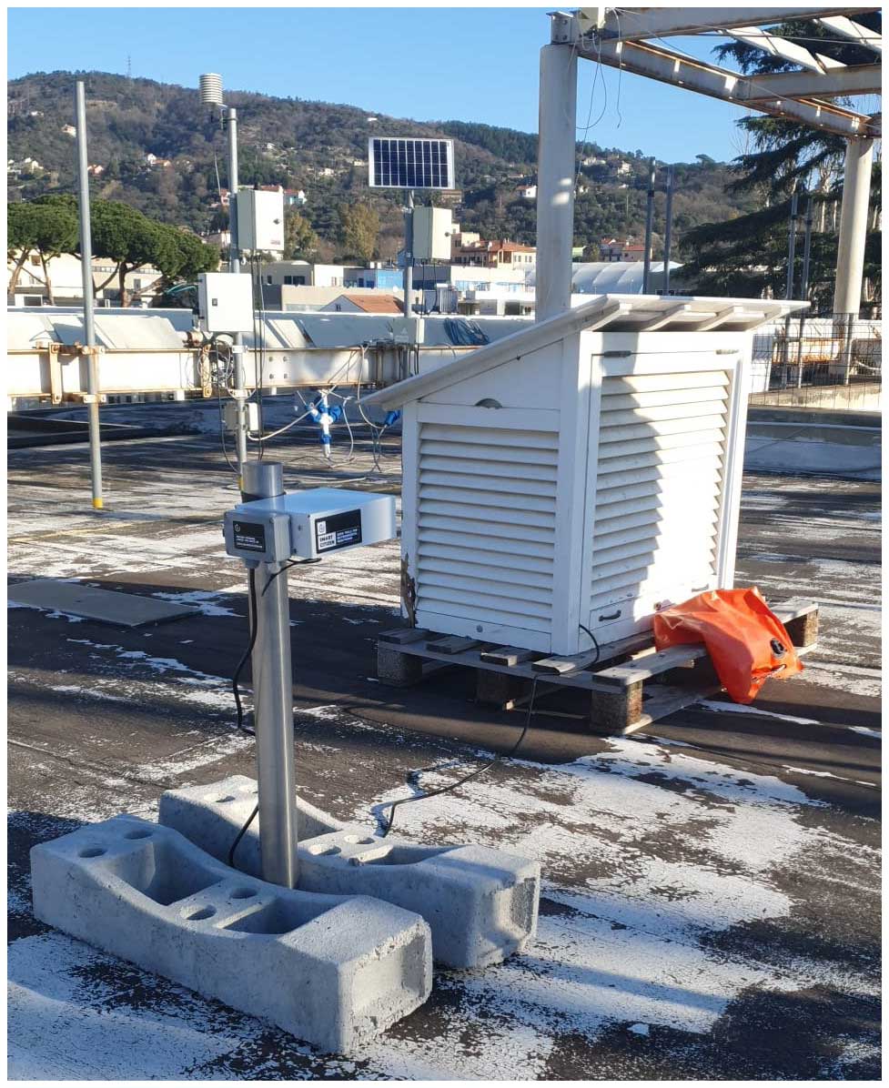
Figure 3 Stevenson screen (front right) and reference weather station (middle back) locations on the building rooftop.

Differently from most of the instrumentation designed for research purposes, the MT operates on the move, introducing a further degree of complexity to the validation procedure. To counteract this limitation, a two-step validation is provided, first using the MT as a fixed-location weather station (Sect. 4.3) and then comparing its performance against a previously validated mobile station (Sect. 4.4). For the fixed-location comparison, an MT was placed behind a Stevenson screen located on the rooftop of the CIMA Research Foundation headquarters (44°17^′59.2^′′ N, 8°27^′06.6^′′ E) close to a reference weather station of the Acronet network. Including the sole sensors required for this study, the reference station is equipped with a shielded transducer (t026 TTEPRH, Siap+Micros S.p.A., Italy) sampling air temperature in the range −30 to +60 °C, with an accuracy of ± 0.1 °C, and relative humidity between 0 % and 100 %, with an accuracy of 2 %. The Stevenson screen is required to shield the MT from solar radiation and to minimize the sensor overheating, thus replicating the work of the RECS when the sensor is moving, to expose the MT to the same environmental conditions as the reference weather station, as deployed in Fig. 3. The data acquisition for this analysis covered two separate periods of continuous measurements, lasting approximately 1 month each: from 19 December 2022 to 10 January 2023 (winter period) and from 11 July to 3 August 2023 (summer period). No weather conditions were discharged from this analysis.

3.4 Mobile comparison

To test the MT under conventional operation conditions, two sensors were mounted on a meteorological cargo bike (see Fig. 4a) developed at Wageningen University (The Netherlands) to measure air temperature, relative humidity, wind speed, and radiation in a reliable way (Heusinkveld et al., 2014).

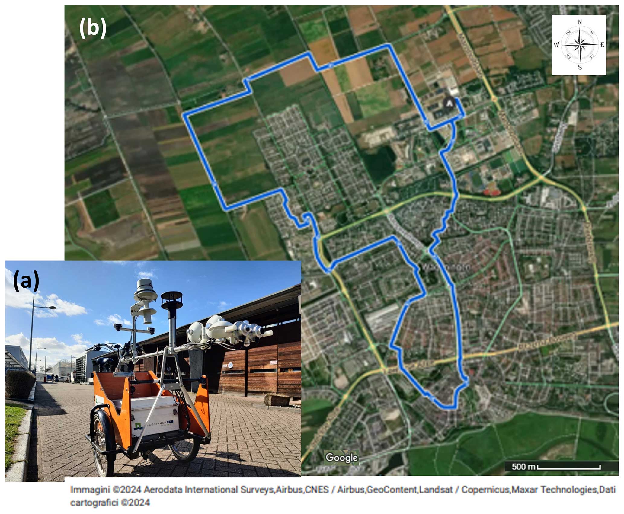
Figure 4 A picture of the cargo bike with its equipment (a) and the cycling route operated for comparison (b).

The temperature and relative humidity are measured with a shielded thermometer–hygrometer (model CS215L, Campbell Scientific, USA) with a radiation screen mounted at 1.2 m. Heusinkveld et al. (2014) ensure an accuracy of less than 0.1 °C for air temperature and 2 % for relative humidity (within the range of 10 %–90 %). Wind speed and direction are measured with a Gill WindSonic (Gill Instruments, UK) and are used to derive the ventilation speed, i.e. the speed of the air sampled by the sensor and given by the vectorial combination of the wind and cargo bike speeds. The MTs were placed unshielded at the same height as the reference temperature sensor, one to its left and the other to its right. With this setup, the average temperature of the MTs corresponds to the reference temperature. The reference temperature sensor samples at 1 Hz; with an average cycling speed of 4 m s⁻¹, it corresponds to a sample every 4 m. The MTs measure with a 3 s sampling rate, resulting in a sample approximately every 12 m. A block average of 5 s is chosen for the comparison.

The data collection was performed in eight sessions from 11 January to 3 March 2023, lasting around 1 h each between 12:00 and 18:00 local time (except for a single evening session starting at 20:30 local time). The dataset encloses different atmospheric conditions, mostly accounting for sunny days when incoming radiation varies the most or for partially cloudy conditions (with no precipitation). The cycling track followed a fixed route, with a seemingly constant cycling speed of 4 ms⁻¹. This cycling route went through an open grassland area near Wageningen (Binnenveld), a new residential area (Wageningen Noordwest), and the historic city centre of Wageningen (see Fig. 4b).

4 Results

4.1 Removal of outliers and adjustment period

From a visual inspection of the data, there are no clear outliers inside the measuring periods. The stability of the MT and its sampling rate minimize the possibility of spikes in the data acquisition, actually preventing the occurrence of outliers within the time series. Conversely, there is clear evidence that, upon activation, the sensor undergoes a process of adjustment to align with the surrounding ambient temperature. Several preliminary tests were implemented during wintertime to investigate the MT's adjustment times according to the different ambient conditions the MT has to adjust to and the cooling rate it has to endure. All these tests were performed by bicycle in Bologna. Equation (2) is applied to isolate and remove these adjustment periods from the data distribution of this test. Figure 5 picks an example session to show the application of the outlier removal method.

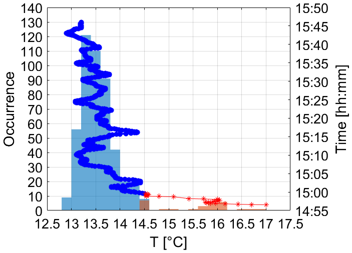
Figure 5 Distribution by the occurrence of the air temperature for the example session, alongside the time evolution of the session. The colours highlight the removed adjustment time after the application of Eq. (2) (blue) compared to the filtered data distribution and time series (red).

The distribution of the air temperature follows a skewed normal distribution, with a bimodal factor when outliers are accounted for. The outliers compose the adjustment period, and no further spikes are detected through the time series. The maximum temperature recorded at the beginning of the session in Fig. 5 is 17.0 °C, falling to 14.5 °C after applying Eq. (2). Similarly, the initial minimum humidity level is recorded at 52 %, but it increases to 59 % during the same time frame as that of the temperature drop after applying Eq. (2) (not shown).

Table 3 summarizes the average temperature changes, adjustment times, and cooling rates evaluated through the preliminary tests and the mobile comparison test performed with the cargo bike (Sect. 3.4).

Table 3 Average air temperature, temperature drop (in absolute value), adjustment time, and cooling rate for the different mobile monitoring sessions involved in the tests. For each session, the date, starting time, and duration are also reported. Comp⁢ sessions are performed in Bologna, and Cargo⁢ ones are from the mobile comparison in Wageningen. Multiple dates and start times refer to the individual days and the beginning of each session, the values of which are averaged.

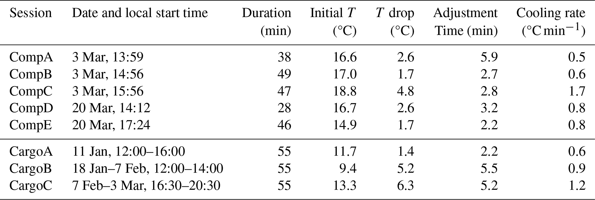
Temperature changes and adjustment times are direct outcomes of the outlier removal, while the cooling or heating rates are computed as their ratios. The discrepancy between adjustment periods and cooling or heating rates is due to the initial air temperature and the different times of the day – and, hence, the intensity of solar radiation. Natural ventilation can also play a role in increasing the cooling rate. Overall, the cooling or heating rate of an MT under operational use ranges between 0.5 to 1.7 °C min⁻¹, accounting for an adjustment time of 2.2–6.3 min according to this test. Table 3 only reports the application of the removal method to the air temperature, but the same procedure has been independently applied to the relative humidity, obtaining similar results. For this reason, temperature alone is taken as a benchmark for identifying the adjustment period.

To provide further support for the acclimatization process of the MT, supplementary comparison tests with an analogue thermometer are carried out both indoors and outdoors. Results of these tests suggest that a stationary MT takes 15 min (on average) to achieve thermal equilibrium in a partially controlled room from an initial temperature discrepancy of 2 °C. When exposed to outdoor conditions, the stationary MT takes 10 min (on average) to drop its temperature of 2 °C. Thanks to the thermal regulation induced by ventilation, the adjustment times are largely reduced when the sensor is moving at a speed higher than 7 km h⁻¹. For the intra-sensor variability test and the fixed-station comparison, we waited 15–20 min after having prepared the experimental setup, letting the MT adjust to the ambient air.

4.2 Intra-sensor variability and data correction methods

The results of the intra-sensor variability analysis are presented alongside the development and application of data-driven correction methods for data post-processing. The scope of the corrections is to decrease the variability of data around the mean and to increase the linear relationship of each track to the mean within the session, thus reducing the intra-sensor variability. In particular, a correction was searched and applied wherever single tracks were consistently over- or under-shooting the range represented by the instrumental error applied to the session average. Session S1 is used as a test case, while S2 and S3 are the benchmark. Data measured by the MTs are averaged every 5 s to remove the discrepancy in the time–space acquisition dichotomy and to homogenize the dataset. For each variable, the average session is computed to explore the stability of each sensor measure around the mean. The comparison for the measured variables is shown in Fig. 6.

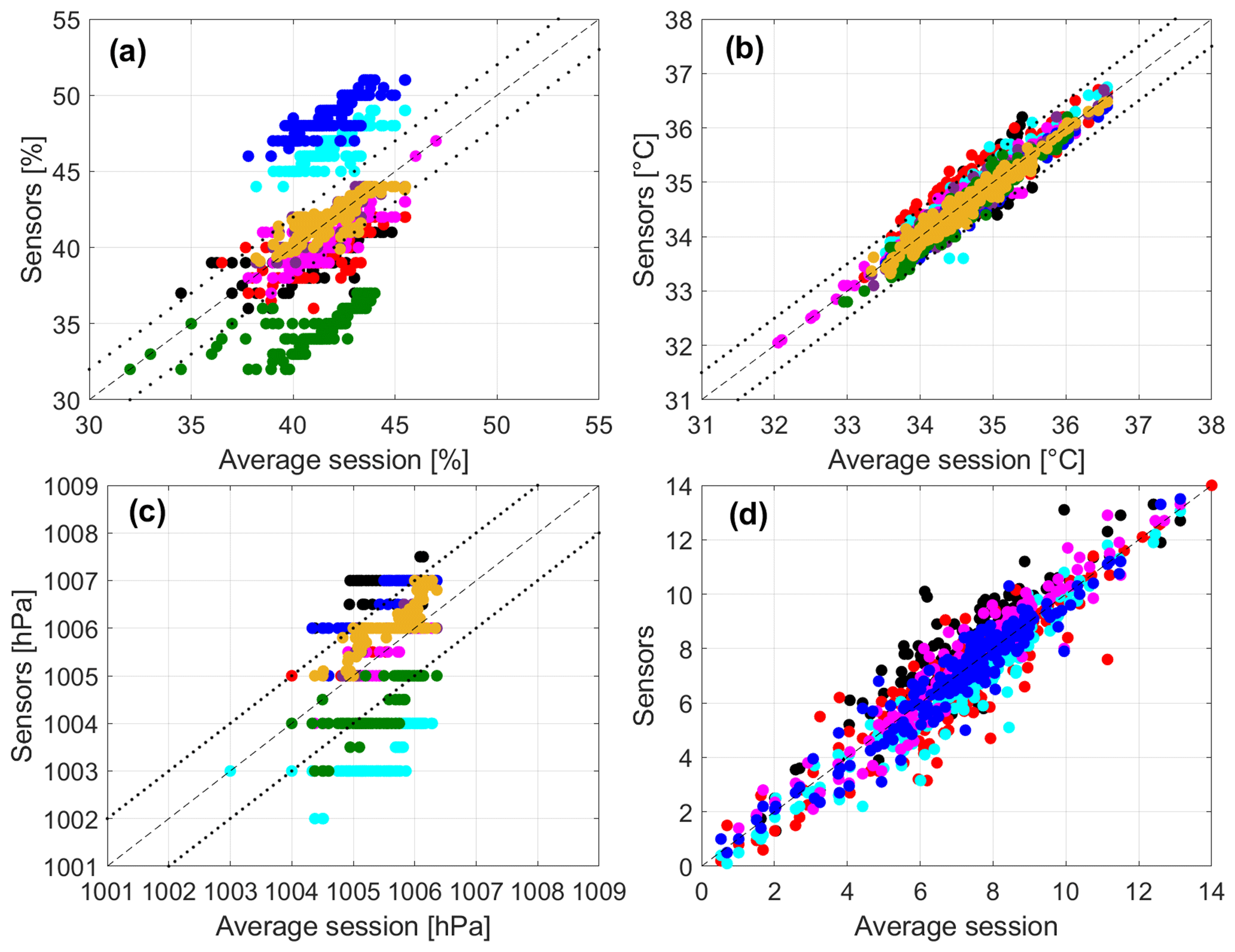
Figure 6 The 5 s averages of relative humidity RH (a), air temperature T (b), barometric pressure P (c), and solar radiation intensity indicator R (d) measured by each sensor as a function of the average session. Each colour identifies the measurement of a single MT. The dashed line is the bisector, and the dotted lines are the instrumental error around the bisector.

As a byproduct, the comparison masks the non-systematic errors while enhancing the existing biases between different measures. This results in large values of the determination coefficient despite the single sensor measurements occasionally being well beyond the range defined by the instrumental error around the average session. This is the case for relative humidity (Fig. 6a) and less so for pressure (Fig. 6c). While, for the pressure, the discrepancy between different sensors accounts for up to 100 % of the instrumental error, that for relative humidity accounts for up to 500 %. Pressure does not display a homogeneous distribution of values around the average session but rather shows a step-wise measurement trend, probably owing to the low sensitivity of the sensor. Air temperatures fall mostly within the instrumental error (Fig. 6b), apart from a few values in two sessions. Air temperature is considered to perform at a level of accuracy in line with the manufacturer's indication and will not undergo any corrections. The solar radiation intensity indicator (Fig. 6d) provides a dimensionless measure of the intensity of solar radiation, with sensors being affected by different shadowing along the track. The performance of this quantity is qualitatively appreciable despite the lack of information on the instrumental error preventing a more quantitative evaluation.

From the measurements described above and the information retrieved from the GPS of the smartphone, the sensor automatically derives several quantities including altitude Z, vehicle speed V_s, the dew point T_d, and the humidex index HDX (see Fig. 7).

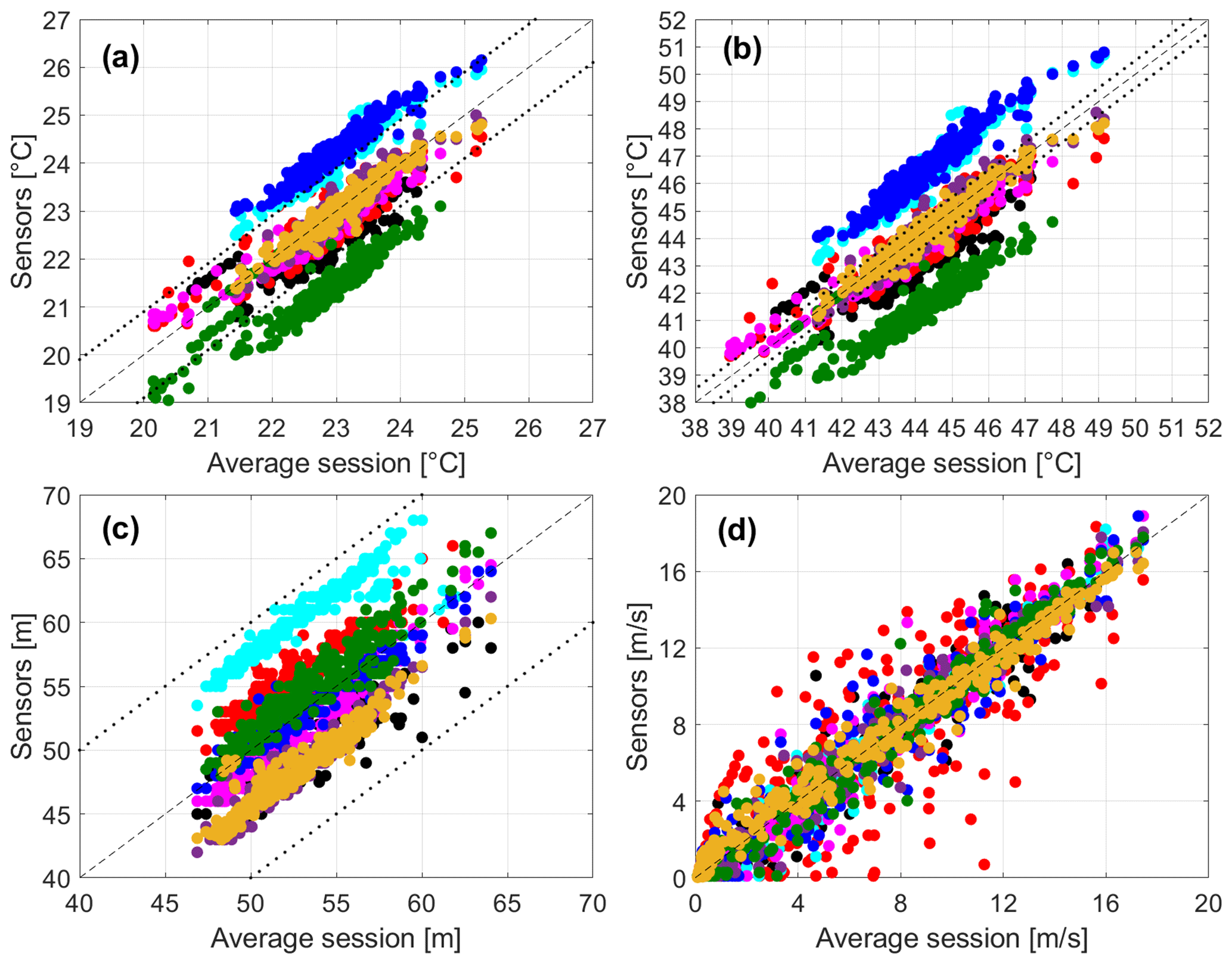
Figure 7 The 5 s averages of the dew point T_d (a), humidex HDX (b), and altitude above mean sea level Z (c) derived by each sensor as a function of the average session, along with the vehicle speed V_s (d) derived from the smartphones' GPSs. Each colour identifies the measurement of a single MT. The dashed line is the bisector, and the dotted lines are the instrumental error around the bisector.

The vehicle speed is self-consistent, despite an increasing spread of values at low velocities (Fig. 6d). Despite the facts that an instrumental error for the vehicle speed is not provided by the manufacturer (as it depends on the smartphone the sensor is connected to) and that a more quantitative assessment of this variable is precluded, this can still be used as an indicator of the stability for different smartphone models. As for the altitude, the phone GPS is involved in the computation of the vehicle velocity; thus, similarities between measurements are expected but not granted.

Altitude above the mean sea level (Fig. 7c) is automatically computed by the MT by retrieving the initial altitude Z₀ from an open web server using the location of the initial latitude and longitude and then modifying its value along the track according to the measured pressure using

$$\begin{array}{}\text{(3)}& Z={\displaystyle \frac{T_{\mathrm{0}}}{{\mathrm{\Gamma }}_s}}\left({\left({\displaystyle \frac{P}{P_{\mathrm{0}}}}\right)}^{-{\mathrm{\Gamma }}_s{R}_{\mathrm{d}}/g}-\mathrm{1}\right)+Z_{\mathrm{0}},\end{array}$$

where T₀, P₀, and Z₀ are the air temperature, pressure, and altitude collected as the first data measure, respectively; Γ_s=0.0065 °C m⁻¹ is the standard atmospheric lapse rate; g=9.81 m s⁻¹ is the acceleration due to gravity; and R_d is the gas constant for the dry air. The nominal error of ± 10 m associated with the altitude measurement is therefore a composition of the error propagation given by Eq. (3) and the GPS accuracy. It is worth noting that the accuracy of the GPS is a property of the smartphone connected to the MT, and it can change according to the smartphone brand and model. Since this test was conducted using different smartphones, we could have introduced an additional source of error. The correction we are about to introduce will minimize this error, but it is arguable that using the same smartphone model and brand the correction would not be needed (at least if the error from Eq. (3) is negligible). The large nominal error allows a good altitude performance within the current test, but biases between sensors are also evident. For this reason, an alternative procedure to compute altitude is proposed. It consists of the retrieval of the altitude from a preferred web server (such as the one used in this paper) or a digital elevation model map for each latitude–longitude couple measured by the GPS, thus bypassing Eq. (3). In other words, the sole error remaining in the computation of the altitude is associated with the GPS signal. This procedure is more computationally expansive than Eq. (3), but it ensures a better evaluation of the altitude as long as the GPS signal is stable. Applied to S1, the method grants a large improvement in the altitude computation, with a drastic reduction in the sessions' spread around the mean one (Fig. 8).

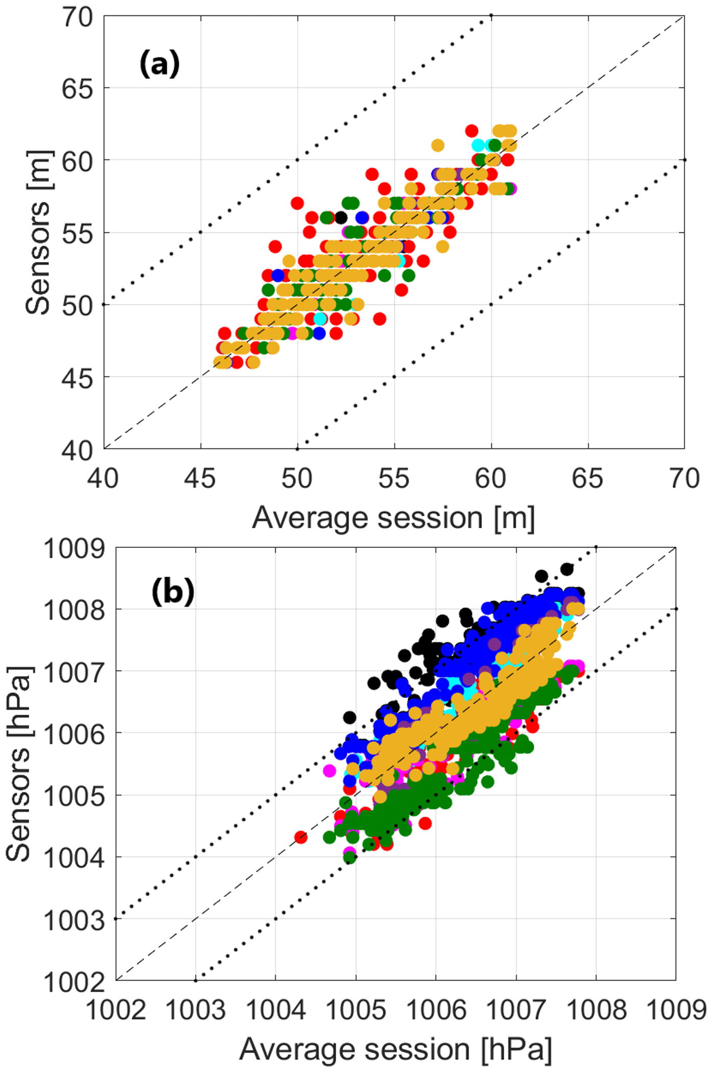
Figure 8 The 5 s averages of the corrected altitude P_c (a) and pressure Z_c (b) as a function of the average session. Each colour identifies the measurement of a single MT. The dashed line is the bisector, and the dotted lines are the instrumental error around the bisector.

The improvement in the altitude values enables the correction of pressure. From Eq. (3), we can derive an expression for pressure P_c as

$$\begin{array}{}\text{(4)}& P_{\mathrm{c}}=P_{\mathrm{0}}{\left({\displaystyle \frac{{\mathrm{\Gamma }}_s}{T_{\mathrm{0}}}}\left(Z_{\mathrm{c}}-Z_{\mathrm{0}}\right)+\mathrm{1}\right)}^{-g/\left({\mathrm{\Gamma }}_s{R}_{\mathrm{d}}\right)},\end{array}$$

where Z_c is the altitude above the mean sea level as retrieved from the web server. The recomputed pressure is shown in Fig. 8. The correction collapses pressure from different sensors within the instrumental range of uncertainty (around the average session) while introducing a richer value distribution. This is supposedly caused by the larger sensitivity of the GPS sensor compared to the barometer.

Using P_c, we can estimate a first correction formula for the relative humidity. The relative humidity is defined as the ratio between the water vapour pressure e and the saturation water vapour pressure e_s. Assuming that the variability of the total pressure is entirely driven by that of the water vapour, δRH∝δe. The application of this correction type to the relative humidity revealed almost negligible results for the dataset under investigation, and, for this reason, it was discarded. Nonetheless, e and e_s are known to be functions of the dew point T_d and the air temperature T, respectively, owing to a large number of empirical (e.g. the Magnus formula) and theoretical (derived from the Clausius–Clapeyron equation) expressions. The link between T, T_d, and RH suggests the possibility of finding correction methods for RH based on these variables, to which the humidex index HDX can be added owing to its dependency on both temperature and relative humidity. Indeed, both T_d and HDX show an odd intra-sensor variability which is propagated from the relative humidity (see Fig. 7a, b), with the dew point being affected the most. From its definitions in Eq. (1), the humidex index depends more on the air temperature and less on relative humidity (or dew point). In the range of temperatures where the humidex is defined, the adding term in the RHS (right-hand side) of Eq. (1) is much smaller than T, and thus the intra-sensor variability in the humidex is less pronounced than T_d and RH. The humidex index can be used as a starting point for the correction procedure, which will ultimately allow us to correct RH, T_d, and HDX. Practical definitions of this index can be retrieved from Eq. (1), following the standard used by Environment and Climate Change Canada:

$$\begin{array}{}\text{(5)}& \mathrm{HDX}=T+\mathrm{0.5555}\left(\mathrm{6.11}{\mathrm{e}}^{\left(L/R_{\mathrm{w}}\left(\left(\frac{\mathrm{1}}{\mathrm{273.16}}\right)\left(\frac{\mathrm{1}}{\mathrm{273.15}+T_{\mathrm{d}}}\right)\right)\right)}-\mathrm{10}\right),\end{array}$$

where L, the latent heat of vaporization, is retrieved from the linear interpolation of T knowing that L(T=0 °C) = 2.501 × 10⁶ J kg⁻¹ and L(T=100 °C)= 2.257 × 10⁶ J kg⁻¹, while R_w=461 J K⁻¹ kg⁻¹ is the gas constant for a moist atmosphere. Alternatively, we can adopt some Magnus formula for e so that

$$\begin{array}{}\text{(6)}& \mathrm{HDX}=T+\mathrm{0.5555}\left(\mathrm{0.06}\mathrm{RH}{\mathrm{10}}^{\mathrm{0.03}T}-\mathrm{10}\right).\end{array}$$

Both empirical equations require T and T_d in degrees Celsius. Figure 9 shows the correlation and dispersion of the humidex calculated with Eqs. (5) and (6) and the one directly computed by the sensor. Each distribution resembles a Gaussian shape, with a high degree of symmetry and mean (and median) values close to 44 °C. Despite Eq. (6) being a better approximation of the HDX retrieved by the sensors, Eq. (5) already reduces the standard deviation of the distribution and thus the intra-sensor variability. Substituting Eq. (5) into (6) and solving for RH, we obtain an expression for the corrected relative humidity RH_c which only depends on the dew point (and air temperature):

$$\begin{array}{}\text{(7)}& {\mathrm{RH}}_{\mathrm{c}}=\mathrm{100}{e}^{\left(\frac{L}{R_{\mathrm{w}}}\left(\frac{\mathrm{1}}{\mathrm{273.16}}-\frac{\mathrm{1}}{\mathrm{273.15}+T_{\mathrm{d}}}\right)\right)}{\left({\mathrm{10}}^{\mathrm{0.03}T}\right)}^{-\mathrm{1}}=\mathrm{100}{\displaystyle \frac{e}{e_{\mathrm{s}}}},\end{array}$$

where e is formulated following Environment and Climate Change Canada, and e_s follows a simplified Magnus formula. From Eq. (5), we can assume that the significant component of the intra-sensor variation in HDX is given by T_d. That is, δHDX∝δT_d. Using the error propagation theory, the variability $\mathit{\delta }\mathrm{HDX}=\left|\frac{d\mathrm{HDX}}{\mathrm{d}{T}_{\mathrm{d}}}\right|\mathit{\delta }{T}_{\mathrm{d}}$. Solving for δT_d, we get

$$\begin{array}{}\text{(8)}& \begin{array}{rl}& \mathit{\delta }{T}_{\mathrm{d}}=-{\displaystyle \frac{R_{\mathrm{w}}}{L}}{\left(\mathrm{273.15}+T_{\mathrm{d}}\right)}^{\mathrm{2}}{\left(\mathrm{3.39}\right)}^{-\mathrm{1}}\\ & e^{-\frac{L}{R_{\mathrm{w}}}\left(\frac{\mathrm{1}}{\mathrm{273.16}}-\frac{\mathrm{1}}{\mathrm{273.15}+T_{\mathrm{d}}}\right)}\mathit{\delta }\mathrm{HDX}.\end{array}\end{array}$$

The dew point is then corrected as

$$\begin{array}{}\text{(9)}& T_{\mathrm{d}}^{\mathrm{c}}=T_{\mathrm{d}}-\mathit{\delta }{T}_{\mathrm{d}}\end{array}$$

and is used to recompute the humidex using Eq. (5). Equations (8), (9), and (5) are computed recursively to minimize the intra-sensor differences of both T_d and HDX. The minus sign in Eq. (8) is introduced to evaluate both positive and negative components of the derivative in the error propagation. After two iterations, the variability around the average session is already greatly reduced (see Fig. 10a, b). Note that the recursive method is intrinsically going to diverge after a large number of iterations, thus imposing a truncation after a few iterations. Here, truncation is done after visualizing the minimum variability, constrained to a range of values in agreement with the measurements. Using the recursive method, we achieved a better agreement between sensors, ensuring a smaller spread of values around the average session and ensuring that they are constrained within the instrumental errors. Here, the instrumental error for the dew point is derived from the approximated relation of Lawrence (2005):

$$\begin{array}{}\text{(10)}& T_{\mathrm{d}}=T-{\displaystyle \frac{\mathrm{RH}-\mathrm{100}}{\mathrm{5}}}.\end{array}$$

By comparing the dew point retrieved by the sensor and that computed using Eq. (10), we observe two similar distributions (see Fig. 11), suggesting we can adopt Eq. (10) for the computation of the dew-point error.

Figure 9 Cumulative density distribution of the HDX index computed using Eq. (5) (solid black) and Eq. (6) (solid blue) and directly by the sensor (solid red). The dashed lines, paired with similar colours, represent the best normal distribution fit for each data source. The number of bins for the discretization is equal to the square root of the total number of data (equal for each distribution).

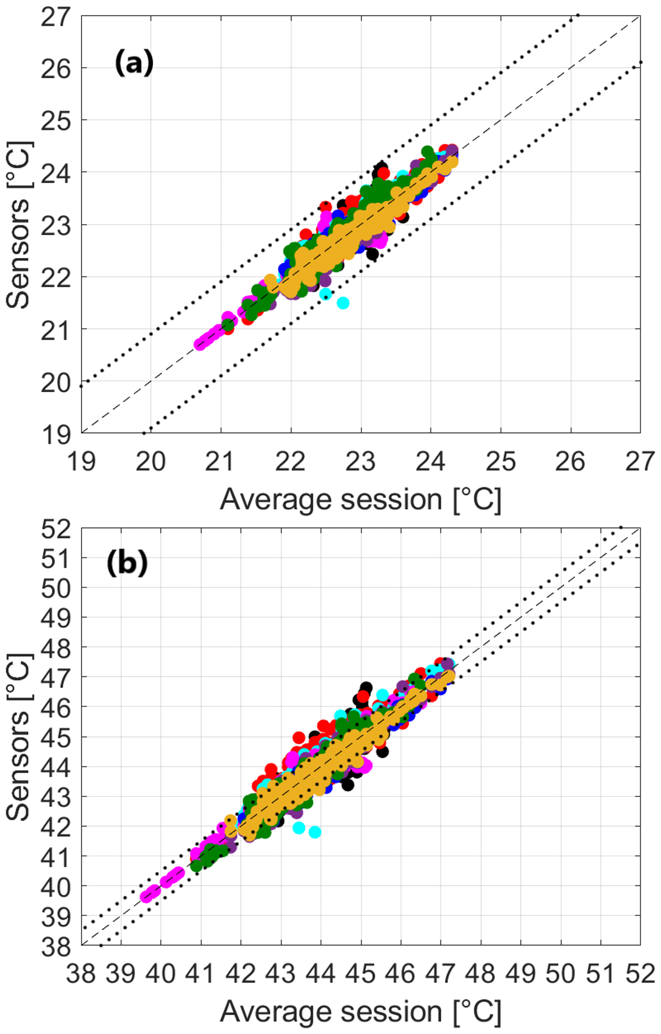
Figure 10 Calculated $T_{\mathrm{d}}^{\mathrm{c}}$ (a) and HDX_c (b) after two iterations using Eqs. (9) and (6) as a function of the average session, respectively. Each colour identifies the measurement of a single MT. The dashed line is the bisector, and the dotted lines are the propagated instrumental error around the bisector evaluated using Eq. (11) for T_d and Eq. (12) for HDX.

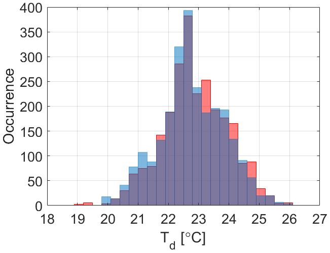
Figure 11 Distribution of the occurrence of the dew point T_d as retrieved from the sensor (red) and computed using Eq. (10) (blue). The purple area of the graph is where the two distributions superimpose one on the other. The bin width is 0.3 °C in an equal number of bins among the distributions.

The agreement shown in Fig. 11 raises doubts about how solid the dew-point data are when directly retrieved by the MT. Equation (10) was suggested by Lawrence (2005) to work in a moist environment, with RH≤50 %, with a possible extension to 40 % introducing a further correction, which was meaningless for the present study. Nonetheless, values below the 40 % threshold were observed, for which we can assume the approximation works just well enough for deriving the dew-point error. In any case, this error evaluation is limited to a medium–high humid environment and should be further tested for more arid conditions. A further assessment of the quality of the dew point retrieved from the sensor is given in Sect. 4.3.

The error associated with the retrieved and corrected dew point reads as

$$\begin{array}{}\text{(11)}& \mathrm{\Delta }{T}_{\mathrm{d}}=\mathrm{\Delta }T+{\displaystyle \frac{\mathrm{1}}{\mathrm{5}}}\mathrm{\Delta }\mathrm{RH}.\end{array}$$

In an analogy, the error associated with the humidex index is computed from Eq. (5) and reads as

$$\begin{array}{}\text{(12)}& \mathrm{\Delta }\mathrm{HDX}=\mathrm{\Delta }T+{\displaystyle \frac{\mathrm{HDX}-\mathrm{T}}{{\left(\mathrm{273.15}+T_{\mathrm{d}}\right)}^{\mathrm{2}}}}{\displaystyle \frac{R_{\mathrm{w}}}{L}}\mathrm{\Delta }{T}_{\mathrm{d}}.\end{array}$$

As dew point and humidex converge to their minimum variability, the corrected value of T_d is used to recompute the relative humidity using Eq. (7), and the resulting difference from the average session is shown in Fig. 12.

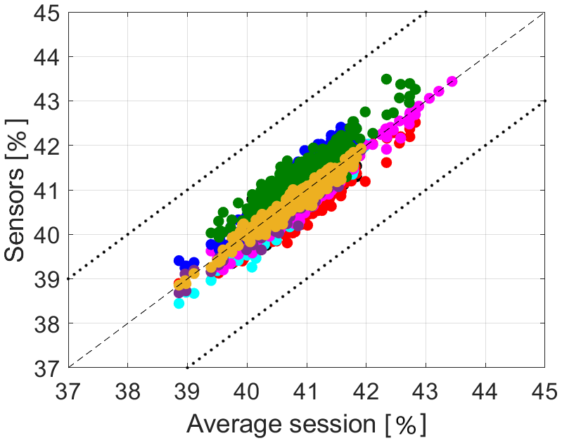
Figure 12 Corrected RH_c using Eq. (7) as a function of the average session. Each colour identifies the measurement of a single MT. The dashed line is the bisector, and the dotted lines are the propagated instrumental error around the bisector.

Despite the fact that the correction is not always sufficient to bring the variability within the instrumental error from the average session (S2, for instance, would have required an error bar of ±3 % – not shown), the intra-sensor agreement is largely improved, as also quantified by the root-mean-square and mean bias errors listed in Table 4 for each session and variable. The correction removes a consistent portion of the sensor variability, producing a maximum value of uncertainty around the average session of ± 1.2 % for S1.

Table 4 Coefficient of determination R², root-mean-square error RMSE, and mean absolute percentage error MAPE computed session by session between the data obtained (measured, derived, or corrected) from each sensor and the respective average session. Below, the average R² within each session and the maxima RMSE and MAPE are reported.

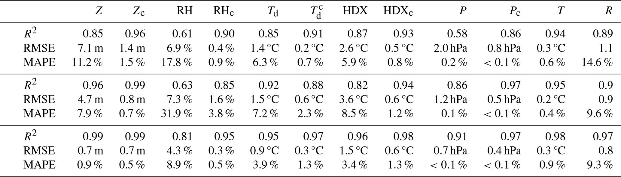
RMSE is calculated as ${\left(\frac{\mathrm{1}}{n}{\sum }_{i=\mathrm{1}}^n{\left(x_i-\langle x_i\rangle \right)}^{\mathrm{2}}\right)}^{\mathrm{1}/\mathrm{2}}$, and MAPE is calculated as $\frac{\mathrm{100}}{n}{\sum }_{i=\mathrm{1}}^n\left|\frac{x_i-\langle x_i\rangle }{x_i}\right|$, with x_i being the iteration of variable x from each sensor, 〈beingx_i〉 the average session of the same variable, n the number of finite data points in x.

All the corrections we have discussed so far have substantially improved the data quality. The absolute errors also decrease, with an overall increase in the determination coefficients. We have already mentioned how the intra-sensor variability assessed here creates a bias in the coefficient of determination due to the dependence of the mean from its constituents. Nonetheless, the initial large values of this coefficient suggest that the existing discrepancy between sensors' measurements is bias-driven, while tendencies are in accordance. The increase in the determination coefficients obtained through the correction methods explains the further reduction in the non-linear uncertainties in the sensors' measurements. The error reduction is instead an indication of the bias decrease; in other words, the sensors' measurements collapse closer to their average.

The pressure–altitude correction encloses both tendency and bias regulation effects. Pressure loses its step-wise conformation, favouring a more homogeneous data distribution which increases the linear dependence between different sensors. Altitude decreases the intra-sensor bias by reducing the mean absolute percentage error (MAPE) of 87 % and 91 %, and the root-mean-square error (RMSE) of 80 % and 82 % in S1 and S2, respectively. The iteration method involving relative humidity, dew point, and humidex is also successful in reducing both biases and tendency discrepancies, especially for the first variable. The largest effect on dew point and humidex is a decrease in the bias around the average, with an efficacy of the correction in the range of 60 %–88 % for both MAPE and RMSE, with a slightly better reduction performance in the humidex. The correction also improves the respective coefficients of determination, but the increase is less impactful, possibly due to the stronger dependence of both variables on the air temperature (which has high scores and did not need any correction) and, less so, on the relative humidity. Finally, the relative humidity experiences the largest benefits from the correction method for both tendency linearity and bias, as is already clear from a visual comparison between Figs. 6a and 12. The linearity around the average session increases by 15 %–30 %, ensuring a more regular distribution of the data and the tendency among different sensors' measures. Even more evident is the improvement by reducing the intra-sensor bias: MAPE and RMSE increase by 78 %–95 %, which is >90 % if we exclude S2, where the correction method was not sufficient to shrink the intra-sensor variability down to be within the instrumental error due to the presence of an “outlier” sensor run. By removing this odd sensor run, S2 aligns with S1 and S3 statistics, allowing rigorous comparability between different MTs' measurements.

4.3 Fixed-location comparison

The intra-sensor variability test has revealed the capability of the MT to perform a self-consistent assessment of the environmental conditions, even though some corrections are necessary to achieve a reasonable performance. In this and the following section, we address the performance of the MT against reference stations both in a fixed location and under optimal usage conditions (i.e. on the move). As introduced in Sect. 3.3, sensors' comparisons during both winter and summer are investigated to verify the consistency of the previous results at both extremes of the annual thermodynamic cycle. We selected periods of continuous measurements without technical issues on both apparatuses. The winter period under investigation has experienced mild weather conditions, with warm temperatures for the season and relative humidity never reaching saturation (according to the reference weather station at the CIMA Research Foundation). Moreover, neither severe nor extreme weather phenomena were observed during the period, thus facilitating the comparability between the MT and the reference weather station. Within the summer of the new global temperature record concerning the warmest July of the measurement era, Savona experienced a warm summer with daily mean and maximum temperatures above the climate average. The period included several heatwaves striking the whole region, while no severe thunder- or rainstorms were observed. The comparison is strictly limited to air temperature and relative humidity as the weather station does not measure any other variable relevant to the MT. An assessment of the dew point and humidex is also provided as both quantities are necessary for the correction of the relative humidity, as we have introduced in Sect. 4.2. To strengthen the statistical robustness of air temperature and relative humidity comparisons, the coefficient of determination is computed for each variable, alongside the mean percentage error (MPE) and the RMSE to address the goodness of the linear fits. Differently from the intra-sensor variability, here, the percentage error is not computed in an absolute value to quantify the over- or underestimation of the MT measurement compared to the reference one. Furthermore, we computed the MPE for the negative and positive differences separately to better appreciate the overall over- and underestimations by the MT. To avoid the miscalculation of MPE for temperature differences across 0 °C, we previously converted the air temperature into Kelvin. Willmott (1981) introduced a decomposition of the mean square error (MSE) into a systematic and an unsystematic component, separating biases from random errors. Following this philosophy, we decomposed the RMSE into its systematic component,

$$\begin{array}{}\text{(13)}& {\mathrm{RMSE}}_{\mathrm{s}}=\sqrt{{\displaystyle \frac{\mathrm{1}}{n}}\sum _{i=\mathrm{1}}^n{\left({\widehat{x}}_i-y_i\right)}^{\mathrm{2}}},\end{array}$$

and its unsystematic component,

$$\begin{array}{}\text{(14)}& {\mathrm{RMSE}}_{\mathrm{u}}=\sqrt{{\displaystyle \frac{\mathrm{1}}{n}}\sum _{i=\mathrm{1}}^n{\left(x_i-{\widehat{x}}_i\right)}^{\mathrm{2}}},\end{array}$$

where x_i is the iteration of variable x from the MT, y_i is that for the reference weather station, n is the number of finite data points in x, and $\widehat{x_i}=a{y}_i+b$ is the linear fit of x to y. The systematic component is the consistent bias that produces the over- or underestimation of the reference values by the MT measurement compared to the linear fit between the two datasets. The unsystematic component evaluates the scatter about the linear regression line of the MT measurements. RMSE is used instead of the MSE for a better comparison with the intra-sensor variability test and the performance evaluations found in the literature (see Sect. 5.2).

Figure 13 compares the air temperature and relative humidity of the MT and the reference station for both winter and summer periods.

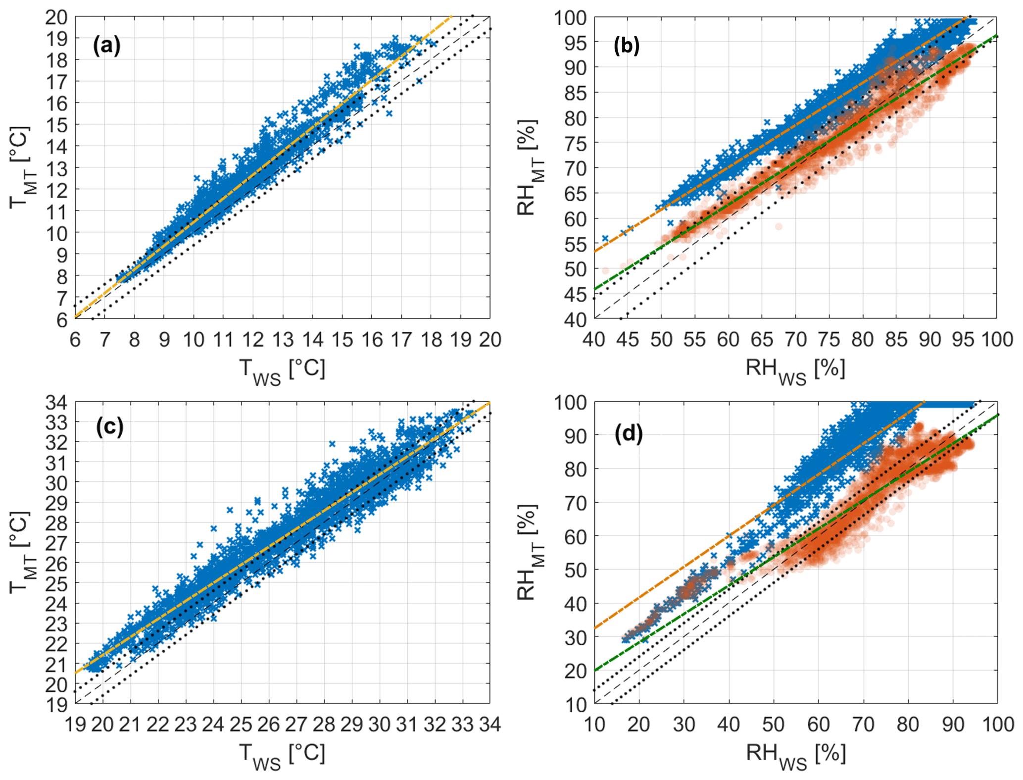
Figure 13 Air temperature T and relative humidity RH comparisons between MT (subscript MT) and reference weather station (subscript WS) measurements for the winter (panels (a) and (b)) and summer (panels (c) and (d)) periods and relative linear fits. In (b) and (d), blue dots and orange fits refer to the measured relative humidity, while red dots and green fits refer to the relative humidity corrected using Eq. (7). The dashed line is the bisector, and the dotted lines identify the range given by the sum of the MT and weather station instrumental errors around the bisector – that is, ± 0.6 °C for air temperature and ± 4 % for relative humidity.

For both quantities, data have been previously processed and averaged every 10 min, and a linear fit is computed as a result of the comparison. During both seasons, the air temperature measured with the MT is in reasonable agreement with the weather station despite a clear tendency to overestimate the reference values. The wintertime overestimation also increases with increasing values of air temperature (Fig. 13a). Apart from the possible intrinsic lack of accuracy of the MT, two factors may affect the performance of the sensor. First, the MT is a mobile sensor used as a fixed meteorological station; i.e. it is operated with a sub-optimal working configuration. Second, the Stevenson screen is not a perfect shield from solar radiation, the beam of which can be reflected from multiple surfaces on the building rooftop into the box volume. In addition, the natural ventilation of the screen is partially prevented by its structure, and air may become stagnant within its volume. It is worth noting that the flat rooftop hosting the experiment is covered with black tarpaulin, thus minimizing the reflection from one of the major sources but increasing the emission temperature of the rooftop, with a larger effect on stagnant air. As a result, the combination of inhibited ventilation and enhanced radiation might increase the air temperature within the screen volume, especially at higher temperatures when we can expect larger solar radiation. Nonetheless, the summertime overestimation is homogeneously distributed along the entire temperature range (Fig. 13c), suggesting that the possible air warming inside the Stevenson screen does not increase linearly with either the air temperature or the solar radiation. Unfortunately, with it being the case that the MT under the screen and the weather station are not equipped for measuring solar radiation, we can only leave these considerations as hypotheses.

The relative humidity measured by the MT is largely overestimated compared to that of the weather station (Fig. 13b, d). Given the outcomes of the intra-sensor variability test, this result is not unexpected. The linear fit of the distribution suggests that the overestimation results from a large bias by the MT. Therefore, we perform a new comparison with the reference station by applying the recursive method to correct the MT measurement. The corrected relative humidity aligns better with the reference values: the tendency remains almost unaltered from the original measurement, and the bias correction is sufficient to provide a more reasonable agreement. As for the intra-sensor variability test, truncation at the second iteration is sufficient to obtain a reasonable performance of the MT under real atmospheric conditions.

For a more quantitative evaluation of the performance of the MT, Table 5 condenses the values for the coefficient of determination and the errors computed for the air temperature, relative humidity, and the corrected relative humidity during both seasons.

Table 5 Coefficient of determination R²; total (RMSE), systematic (RMSE_s), and unsystematic (RMSE_u) root-mean-square errors; and total (MPE), positive (MPE_P), and negative (MPE_N) mean percentage errors computed between the measurements of the MT used as the predictor (x) and those of the weather station used as a reference (y).

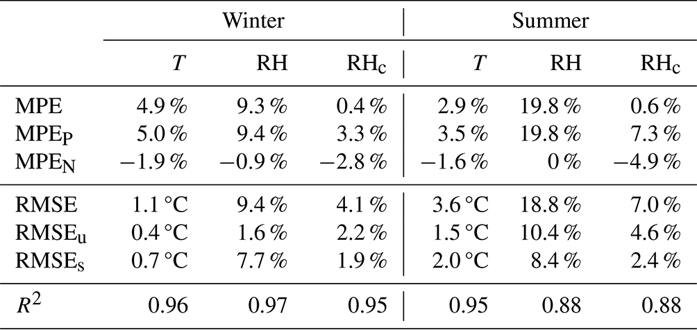
RMSE is calculated as ${\left(\frac{\mathrm{1}}{n}{\sum }_{i=\mathrm{1}}^n{\left(x_i-y_i\right)}^{\mathrm{2}}\right)}^{\mathrm{1}/\mathrm{2}}$, and MPE is calculated as $\frac{\mathrm{100}}{n}{\sum }_{i=\mathrm{1}}^n\frac{x_i-y_i}{x_i}$, with x_i being the iteration of variable x from the MT and y_i being that for the reference weather station, while n is the number of finite data points in x. MPE_P and MPE_N are computed similarly to MPE but summing only the positive and negative values of MPE, respectively.

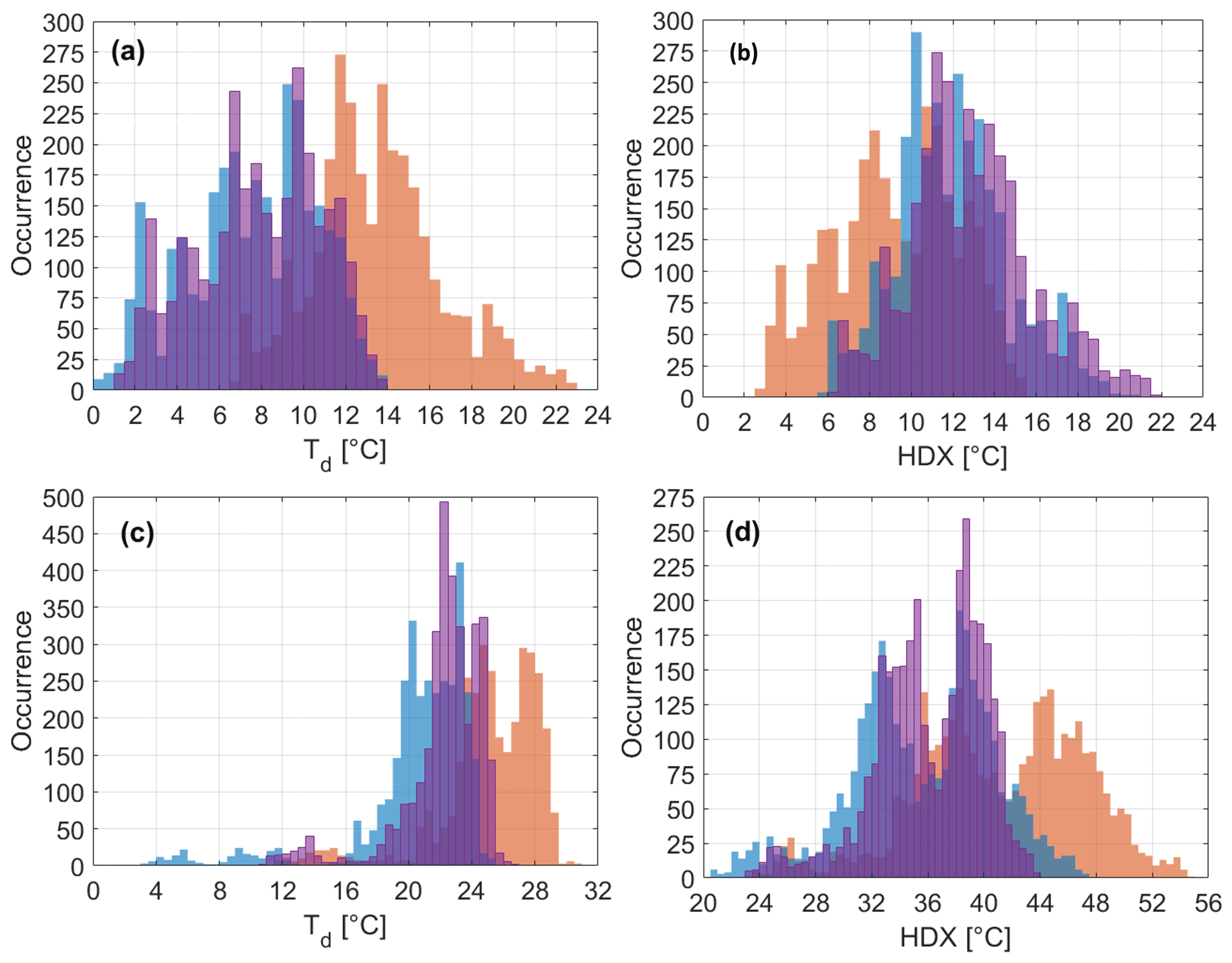
Figure 14 Dew point T_d (a) and humidex HDX (b) distribution comparisons between the variables directly computed by the MT (red), the variables derived from the weather station data using Eq. (15) for T_d and using Eq. (6) for HDX (blue), and the variables obtained after two iterations of the recursive method seen in Sect. 4.2 (purple). Panels (a) and (b) refer to the winter period, and panels (c) and (d) refer to the summertime. The bin width is 0.5 °C on an equal number of bins among the distributions.

All three variables score a high linear correlation with the reference, with a clear tendency of the MT to overestimate the reference values. Winter air temperature shows a positive percentage error, as witnessed by the measurement bias for 67 % and the random error for 33 % (computed as the ratios RMSE_s/RMSE and ${\mathrm{RMSE}}_{\mathrm{u}}/$RMSE, respectively). Similar behaviour is found for the relative humidity, with an even larger percentage error entirely owed to its positive branch and a large RMSE_s over the RMSE_u (${\mathrm{RMSE}}_{\mathrm{s}}/$RMSE ≫ ${\mathrm{RMSE}}_{\mathrm{u}}/$RMSE). The correction adopted for the relative humidity reduces the distribution errors, favouring a larger balance between over- and underestimation, as well as between bias and random errors. The correction severely reduces the total percentage error of relative humidity, balancing positive and negative errors that, on their, own are smaller than the MPE for the air temperature. The correction also reduces the error due to the bias to a value that is smaller than the random error, with the RMSE_s being caused by the remaining overestimation tendency at small relative humidities (see Fig. 13b). During summer, the MPE quantifies the air temperature overestimation at 2.9 % of the measurement, with an overall reduction in the percentage error compared to the winter period. Once again, the discrepancy for air temperature is distributed over a bias responsible for the overestimation (accounting for 55 % of the error) and the random error responsible for the distribution spread around the reference value (45 %). The linearity of the fit is respected. The relative humidity measured with the MT overestimates the reference by 20 % on average (see MPE in Table 5), being entirely outside the instrumental error (Fig. 13d). This causes the MT to observe multiple saturation conditions, while the reference relative humidity rarely exceeds 90 %. The Stevenson screen and the reduced ventilation inside it can favour stagnant conditions, thus increasing the relative humidity. However, the variability observed in the measure of the relative humidity during the intra-sensor variability test hinders this assumption. The RMSE and its components describe a discrepancy from the reference which is larger than the winter period, mostly due to the unsystematic error. This is caused by the large numbers of values at saturation that the MT detects, while the reference station observes relative humidities in the range of 70 %–95 %. In addition to the distribution spread, a bias is also evident, but the linearity of the fit is respected. With the usual two iterations of the correction method, we observe a huge improvement in the agreement between MT and weather station data. Relative humidities below 50 % seem unaltered by the correction. Small values of relative humidity linked with large values of air temperature imply that humidex is determined mostly by the second quantity and less so by the first (see Eq. 6). Since the MT temperature does not change in the recursive method, δHDX and δT_d are small, as are $T_{\mathrm{d}}^{\mathrm{c}}\to T_{\mathrm{d}}$ and RH_c→RH. This shortcoming of the correction did not occur during the intra-sensor variability test as the maximum air temperature was 8 °C smaller than this investigation in Savona.

The recursive method enables us to further discuss the dew point and humidex index. Neither quantity is measured by the weather station, but they can be retrieved using known empirical formulations and then compared with those retrieved directly from the MT and computed through the iterations. Specifically, the dew point T_d for the weather station is derived according to the Magnus formula so that

$$\begin{array}{}\text{(15)}& T_{\mathrm{d}}={\displaystyle \frac{c_{\mathrm{1}}\left(\ln \left(\frac{\mathrm{RH}}{\mathrm{100}}\right)+\frac{c_{\mathrm{2}}T}{c_{\mathrm{1}}+T}\right)}{c_{\mathrm{2}}-\ln \left(\frac{\mathrm{RH}}{\mathrm{100}}\right)-\frac{c_{\mathrm{1}}T}{c_{\mathrm{2}}+T}}},\end{array}$$

where c₁=243.04 °C and c₂=17.625 °C according to Alduchov and Eskridge (1996). This formulation is consistent with a relative humidity resulting from the ratio of water vapour partial pressure and its value at saturation and is in line with other formulations based on the Clausius–Clapeyron equation (Lawrence, 2005). For consistency, the humidex from the weather station is computed by using a Magnus formulation as well according to Eq. (6).

Figure 14 displays the distributions of the MT (directly derived by the sensor), the weather station (Eqs. 15 and 6), and iterated values of T_d and HDX. The distributions of MT data and data retrieved using the weather station share similar shapes but with a bias shifting one from the other. The dew point from the MT overestimates the distribution from the weather station, while an underestimation is observed in the humidex. This turnover is due to the formulations adopted for T_d and HDX, with the first being largely dependent on RH (where the MT largely overestimates the weather station) and the second being more dependent on T. During summer only, the distributions are shaped similarly, with the dew point resembling a skewed normal distribution with a longer left tail, while the humidex is a bimodal distribution covering the whole range of the index. The recursive correction method adopted for RH re-scales the distributions of T_d and HDX, aligning them to the weather station's ones with seasonal discrepancies. During winter, the corrected distributions display longer tails and fewer occurrences at the peaks, but they provide a general improvement in line with the relative humidity. During summer, the corrected distributions encompass restricted ranges and more occurrences at the peaks.

The comparison obtained for these winter and summer periods accomplishes the two goals of this whole investigation:

• The recursive method to correct the relative humidity is proven to be resourceful in retrieving the true relative humidity of the ambient air, along with a reasonable estimation of the dew point and humidex index.

• The MT can capture the thermo-hygrometric properties of the ambient air with an outdoor accuracy that resembles that of the reference weather station but overshoots the combined instrumental errors.

These accomplishments support the use of the MT as a fixed weather station (under customized shielding conditions) to monitor the mean thermal and hygrometric state of the atmosphere.

4.4 Mobile comparison

The final test to assess the MT's data quality is performed under the normal operational mode of the sensor. An instrumented cargo bike is used as a benchmark for air temperature and relative humidity data quality, as described in Sect. 3.4. The comparison is performed by incorporating the measurements from all eight cycling sessions into a single dataset. The statistical characteristics of each variable pair (MT and cargo bike) were computed for this single dataset. As we will argue in this section, we believe the loss of information from each session is not relevant for the quality test since there is not a clear change in behaviour in their data distribution. Only the coefficient of determination is truly overestimated considering the single dataset; for this reason, it is not computed.

Figure 15 shows the air temperature measured by the MT as a function of that from the cargo bike. The temperature range of each session is contained within 1 °C despite the cycling path covering both the city centre and the surroundings of Wageningen. Several ambient factors can be responsible for this small thermal excursion, but they are beyond the scope of this investigation. The key information is that the MT captures the same thermal excursions within the entire temperature range collected during the cycling sessions. Moreover, the majority of the temperature data fall into the error range across the bisector of the comparison, entailing a better quality of data distribution compared to the results for the fixed-location comparison (see Sect. 4.3). A small tendency to overestimate the air temperature from the cargo bike can be observed for each cycling section (Fig. 15). The linear fit displays this overestimation, suggesting the presence of an average bias of 0.3–0.5 °C in the MT data (which remains within the instrumental error range of the MT and cargo bike sensor combined).

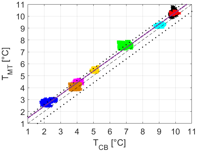
Figure 15 Air temperature T comparison between MT (subscript MT) and cargo bike (subscript CB) measurements, including all the cycling sessions, with each of them identified by a separate colour. The dashed purple line is the linear best fit. The dashed line is the bisector, and the dotted lines identify the range given by the sum of the MT and cargo bike instrumental errors around the bisector – that is, ± 0.6 °C.

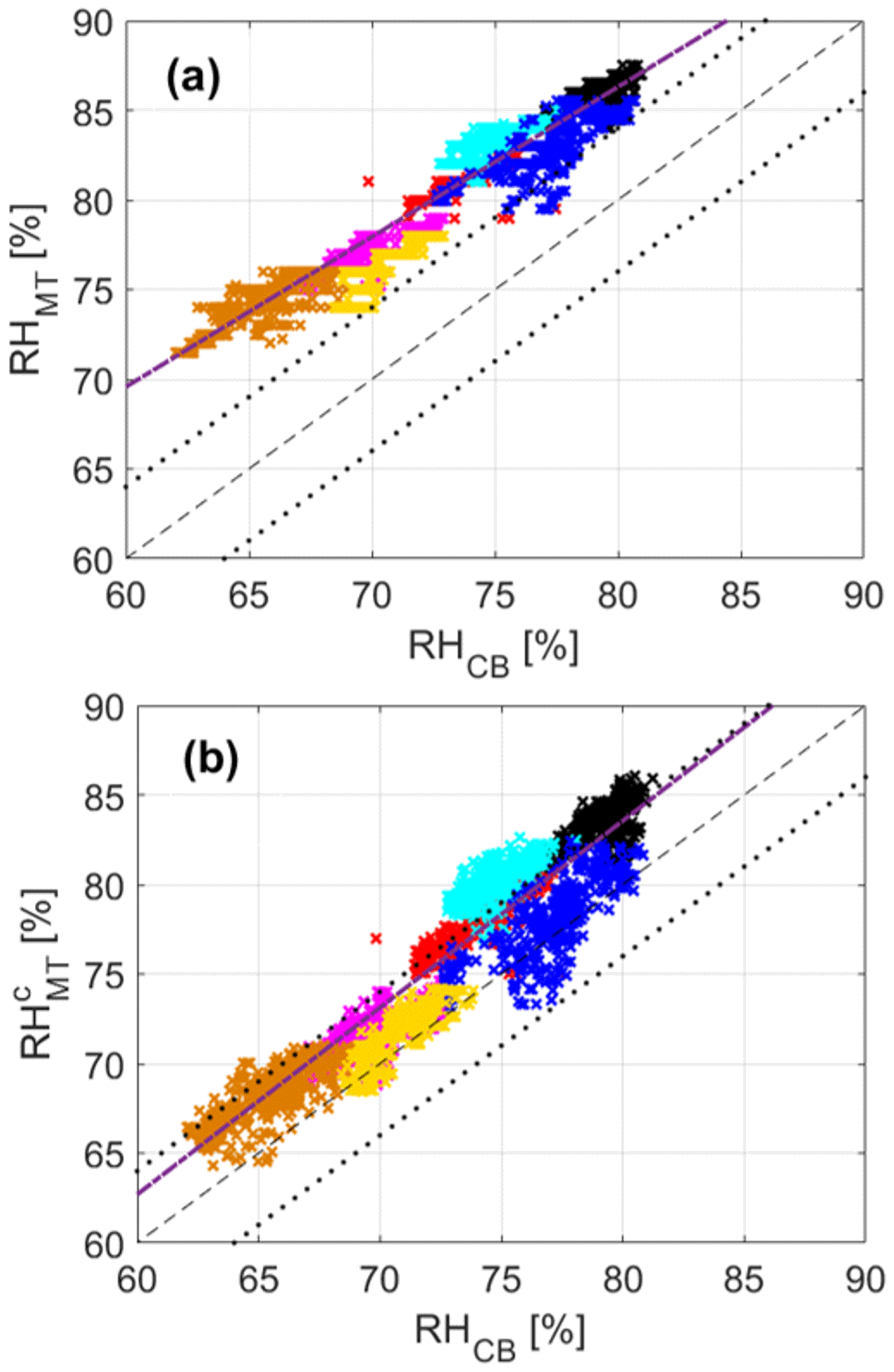
Figure 16 Measured RH and corrected RH^c relative humidity comparison between MT (subscript MT) and cargo bike (subscript CB) measurements, including all the cycling sessions, with each of them identified by a separate colour. The dashed purple line is the linear best fit. The dashed line is the bisector, and the dotted lines identify the range given by the sum of the MT and cargo bike instrumental errors around the bisector – that is, ± 4 %.

The relative humidity measured by the MT shows the well-known overestimation problems we have observed during the previous tests (Fig. 16a). Relative humidity from the MT is consistently outside the error range across the bisector in comparison with the cargo bike, and the overestimation increases with decreasing relative humidity. This behaviour is also observed during the winter period of the fixed-location comparison, where the increasing overestimation of the reference station data at a smaller relative humidity was associated with an increasing overestimation at larger air temperatures (see Fig. 13a). Under fair weather, the typical behaviour for air temperature is to increase when relative humidity decreases and vice versa. Therefore, an overestimation at a large temperature would call for an overestimation at a small relative humidity, as observed. However, the result of the cargo bike test shows that air temperature and relative humidity are completely disjointed and that the performance of the temperature sensor is, once again, far better than that of the relative humidity. Applying the recursive method, the corrected relative humidity improves the agreement with the cargo bike data. Both the overestimation and the increasing discrepancy at smaller values are partially corrected, with a general improvement in the MT data quality. Most of the corrected values of relative humidity fall into the error range, and the fit becomes almost parallel to the bisector.

Table 6 Total (RMSE), systematic (RMSE_s), and unsystematic (RMSE_u) root-mean-square errors; total (MPE), positive (MPE_P), and negative (MPE_N) mean percentage errors; and mean absolute error (MAE) computed between the measurements of the MT used as the predictor (x) and those of the weather station used as a reference (y). Values are computed including all cycling sessions.

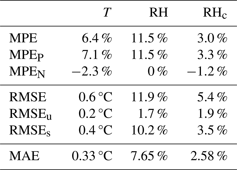
RMSE is calculated as ${\left(\frac{\mathrm{1}}{n}{\sum }_{i=\mathrm{1}}^n{\left(x_i-y_i\right)}^{\mathrm{2}}\right)}^{\mathrm{1}/\mathrm{2}}$, MPE is calculated as $\frac{\mathrm{100}}{n}{\sum }_{i=\mathrm{1}}^n\frac{x_i-y_i}{x_i}$, and MAE is calculated as ${\sum }_{i=\mathrm{1}}^n|x_i-y_i|$, with x_i being the iteration of variable x from the MT and y_i being that for the reference weather station; n is the number of finite data points in x. MPE_P and MPE_N are computed similarly to MPE but summing only the positive and negative values of MPE, respectively.

As for the fixed-location comparison, the MPE (total, positive, and negative branches) and the RMSE (total, systematic, and unsystematic) are computed, and their values are listed in Table 6. Air temperature shows MPEs and RMSEs in line with the winter period of the fixed-location test (see Table 5). The errors fairly describe the overestimation trend ($\mathrm{MPE}>{\mathrm{MPE}}_{\mathrm{P}}\gg {\mathrm{MPE}}_{\mathrm{N}}$) as a result of the MT positive bias in the air temperature (RMSE_s≫RMSE_u). The improvement introduced with the recursive method (after two iterations) is quantified by the error differences between RH and RH_c. The overestimation problem of the MT remains even after the correction application, but its amplitude is drastically reduced. The recursive method decreases the MPE (both positive and total) by 73 % and the RMSE (total and systematic) by 86 %. The positive bias between the MT and the cargo bike remains as the slight increase in the random error fraction ${\mathrm{RMSE}}_{\mathrm{u}}/\mathrm{RMSE}$ is not sufficient to counterbalance the relation of $\mathrm{RMSE}\ge {\mathrm{RMSE}}_{\mathrm{s}}\gg {\mathrm{RMSE}}_{\mathrm{u}}$ observed for the measured RH. As for the air temperature, the corrected relative humidity has statistical errors in line with the fixed-location test (worse than winter and better than summer periods).

To further investigate the reasons for the overestimation, we inspect the incoming solar radiation and ventilation speed measured by the cargo bike. Being unshielded and unventilated, the MT can increase the temperature of its case or that of the air sampled when stagnant. Both conditions can lead to an overestimation of the air temperature and uncertain implications for the relative humidity despite the software correction of the RECS. On the one hand, the increasing temperature of the sensor case can dry the air sample, reducing the relative humidity. On the other hand, stagnation can lead to saturation and an increase in relative humidity. To investigate the impact of both quantities on the sensor performance, the percentage deviation of air temperature and corrected relative humidity are computed as

$$\begin{array}{}\text{(16)}& {\mathrm{\Delta }}_{\mathit{\%}}=\mathrm{100}{\displaystyle \frac{{\mathit{\chi }}_{\mathrm{MT}}-{\mathit{\chi }}_{\mathrm{CB}}}{{\mathit{\chi }}_{\mathrm{MT}}}},\end{array}$$

where χ is either T or RH^c, and the subscripts refer to the MT (MT) or the cargo bike (CB). An average among bins of incoming solar radiation serves as a bin-driven MPE (named bin-averaged percentage deviation) to compare with those in Table 6. Specifically, the MPE is computed within bins of 50 W m⁻², averaging the Δ_% for each variable. Figure 17 displays the percentage deviations as a function of the incoming solar radiation and the ventilation speed.

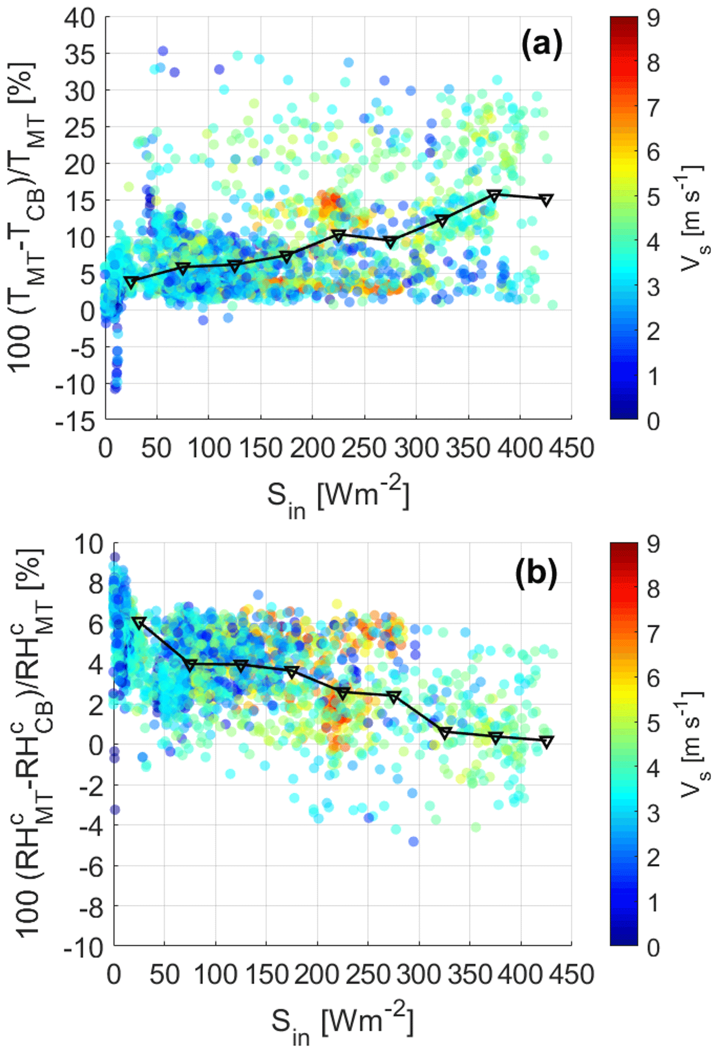
Figure 17 Percentage deviation of air temperature T (a) and corrected relative humidity RH^c (b) as a function of the incoming shortwave radiation S_in and the ventilation speed V_s, including all the cycling sessions. The black line with diamonds is the MPE computed on each 50 Wm⁻² bin of incoming shortwave radiation and is plotted in the middle of the bin.

As a common feature, air temperature and relative humidity deviations cover a large range of variability. Temperature distribution displays a positive trend, increasing the overestimation of the MT with increasing radiation. For solar radiation in the range of 0–200 Wm⁻², the bin-averaged percentage deviation is close to the MPE retrieved for the whole distribution, describing a positive bias below 8 % compared to the cargo bike. At the radiation peak of the investigated period, the bin-averaged percentage error is almost 15 %, doubling the low-radiation condition. On the contrary, relative humidity has a negative trend, decreasing the MT deviation from the cargo bike with increasing radiation and reaching an overturning of the deviation sign starting at 200 Wm⁻². The bin-averaged percentage deviation is approximately 1 % higher than the MPE in the range of 0–200 Wm⁻² while decreasing below a value of 1 % above 300 Wm⁻². The ventilation speed does not show a neat impact on either temperature or relative humidity. At 200–250 Wm⁻², the percentage deviation of air temperature increases with the ventilation speed while decreasing within the previous and following 50 Wm⁻² bins. Once again, the relative humidity deviation behaves in opposition to air temperature.

The comparison with the measurements from the cargo bike has proven the following:

• The recursive method is a resourceful tool for retrieving the true relative humidity of the ambient air under the standard working conditions of the MT.

• The MT tendency to overestimate both air temperature and relative humidity (mostly within the instrumental error) is a shortcoming of the sensor not induced by external factors (e.g. non-standard operational conditions).

• The MT can capture the thermo-hygrometric properties of the ambient air while operating on the move with an accuracy that resembles a certified mobile weather station but that overshoots the combined instrumental errors.

These accomplishments support the use of the MT as a mobile weather station to monitor the mean thermal and hygrometric state of the atmosphere.

5 Discussion

5.1 Notes on the recursive method

The recursive method is the correction introduced to modify the value of the relative humidity through an iterative correction of the dew point and the humidex. The underlying hypothesis of this method is that the modification imposed on the dew point is proportional to those on the humidex and relative humidity, with air temperature being constant. This hypothesis is most likely true as soon as the modification is small since relative humidity can oscillate around a constant air temperature. The performance of the MT temperature sensor also suggests that large modifications can be possible, with those being related to a bad MT performance in measuring relative humidity rather than real atmospheric variability. However, no physical principles support this method; it is rather a tentative solution to adjust a biased sensor.

Being based on the error propagation theory, the recursive method is divergent by definition. Both corrective terms δT_d and δHDX are positive at each iteration, rapidly bringing RH_c to unrealistic values. The introduction of a negative sign in the δT_d equation alternates from positive to negative contributions to T_c; nonetheless, Fig. 18 shows a slow but continuous decrease in the RH_c, with a divergent ending after several iterations. Note that the first iteration is only needed to reproduce the measurements so we can argue that the true iteration is i−1. The number of iterations required to reach a non-physical value of RH_c depends on the reciprocal variation of air temperature and relative humidity. In the specific case of Fig. 18, as RH increases from 0 % to 100 %, T decreases from 45 to −5 °C, covering a full range of realistic values for mid-latitudes. This implies a perfect scenario where air temperature and relative humidity are perfectly (and inversely) correlated, while reality mostly shows oscillations of air temperature around each value of relative humidity and vice versa. A more complex variation in air temperature with relative humidity modifies the effect of the recursive method, amplifying or decreasing its impact at different values of RH. Nonetheless, the scope of this section is to argue on the divergent nature of the recursive method. Breaking the recursive method after a few iterations is therefore fundamental to avoid the result divergence and to ensure that the final RH_c is “close” to the original RH. In a way, a small number of iterations constrains RH_c to RH. For the tests conducted in this paper, the recursive method only necessitated two iterations, involving a small decrease in relative humidity compared to the original measurement. Although the number of tests is limited, the constant number of iterations used to reach the best agreement with the reference can be a recipe for future applications.

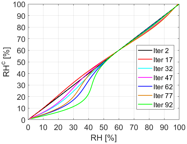
Figure 18 Corrected relative humidity RH_c as a function of the measured RH at different iterations. The recursive method is built over the full RH range and for air temperatures between −5 and 45 °C. The dashed line is the bisector.

5.2 Performance comparison with other mobile sensors

The world of mobile sensors and stations comprises many suites, ranging from research-grade instruments mounted on moving carriers to low-cost sensors specifically designed for mobile sensing. This comes with a variety of nominal (i.e. evaluated by the manufacturer through laboratory testing under ideal measuring conditions) accuracies that depend on the quality of the sensor's suite. From the literature survey of this paper, the accuracy ranges between ± 0.1 to ± 1 °C for air temperature and ± 1.5 % to ± 5 % for relative humidity, with the MT falling into these ranges. Under outdoor ambient conditions, operating a sensor with a non-optimal setup (e.g. a sensor designed for monitoring in a fixed location used as a mobile device) or using a low-cost sensor decreases the chances of meeting the manufacturer accuracy due to the response time of the instrument to the non-stationarity of the ambient air. In this section, we contextualize the performance of the MT in comparison with its reference to other validation studies for mobile sensors from the literature. Although we are aware of the limits of compatibility of the different mobile sensors and the comparability of the collected data (Schering et al., 2022), this comparison serves as a qualitative way to rank the performance of MTs compared to their competitors. We will take the results obtained for the mobile comparison (Table 6 in Sect. 3.4) as the sensor was used under a normal operational mode. Considering sensors usually mounted in fixed stations, HOBOs (Onset Computer Corporation, USA) are the most widely used for mobile sensing due to their compact design, moderate cost, and research-grade reliability. Among those, Qi et al. (2022) adopted a shielded HOBO MX2302 (air temperature accuracy of ± 0.2 °C) mounted on a cart at 1.5 m a.g.l. Along the measuring track, the cart passed 14 fixed stations in the area used as a reference. The comparison showed that 80 % of measurements were in the accuracy range of the instrument and that the MAE after reaching the optimal measuring setup was in the range of 0.14 to 0.62 °C, in line with this paper. Tsin et al. (2016) used a shielded temperature sensor (Met One 064-2, with an accuracy of ± 0.1 °C sampling at 10 s) mounted on a pipe, employing walking sampling; a comparison with a fixed station nearby revealed an underestimation in the range of 2 °C and a poor agreement with data from Landsat (with a coefficient of determination R² of 0.04–0.38). Crowdsourcing air temperature using Netatmo urban weather stations (https://www.netatmo.com, last access: November 2023), Meier et al. (2017) obtained an RMSE in the range of 0.5–1.5 °C for spatially aggregated raw data for hourly and daily urban air temperatures. A better performance was obtained by Liu et al. (2017), who opted for a shielded HOBO-THB-M002 (air temperature accuracy of ± 0.2 °C) mounted on a bicycle, obtaining an RMSE and MAE within 0.3 °C when comparing the local UHI intensity obtained from mobile sensors and that from nine reference stations along the track. The bicycle is among the top choices for mobile sensing, combining a good spatial coverage of the investigated domain and a low moving speed facilitating the comparison with the fixed reference. The bicycle is also a practical solution for low-cost sensors owing to the low-cost philosophy (no emission, low if no energy consumption, small price of the vehicle). Rodríguez et al. (2020) developed and tested a self-made temperature sensor, obtaining a deviation from the fixed reference along the path in line with the sensor accuracy (± 0.5 °C). Worse results were obtained by Vieijra et al. (2023), approaching the accuracy (± 1 °C) with an air temperature device based on the Adafruit BME280 sensor (developed by Bosch) when compared with fixed references.

Other authors preferred to derive the real accuracy of the mobile sensor in isolated chambers before using it in the field. Although close to ideal conditions, this test offers a second accuracy computation independently from the manufacturer. Selected chambers for the scope are calibration ovens (Skoulika et al., 2014) and isolated chambers (Cao et al., 2020), where variations in temperature and humidity are controlled. In the study by Skoulika et al. (2014), the real accuracy of the BC15 thermo-hygrometer sensor (TROTEC International GmbH & C. S.a.s.) was estimated to be in the range of ± 0.2 to ± 1 °C, while Cao et al. (2020) reached a maximum real accuracy of ± 0.48 °C and ± 1.9 % for the sensor suite unit Smart-T (developed at Yale University). Although we cannot perform a similar experiment, we can conduct an evaluation based on the field experiment, knowing that we were exposed to a higher and faster ambient variability than the laboratory tests. Being a mean approximation of data distribution, the linear fit for air temperature and relative humidity from the mobile test can be used to infer the outdoor accuracy of the MT. We can argue that the outdoor accuracy for air temperature is in the range of ± 0.3 to ± 0.5 °C, while the corrected relative humidity ranges between ± 3 % and ± 5%, with both values being in line with the ranges depicted in the literature.

Finally, Cecilia and Peng (2022) performed a first validation test of the MT, monitoring the air temperature and relative humidity against two 5400 WBGT Heat Stress Trackers (Kestrel Instruments) on a bicycle path travelled along at low speeds. The comparison showed a large agreement between the MT and its references, with a coefficient of determination for both variables of R²=0.74 compared to R²=0.64, obtained as an average of all sessions performed within the carbo bike experiment of this paper.

6 Conclusions

This paper explores the outdoor performance of a novel mobile sensor in performing consistent measurements of atmospheric microclimate characteristics. The sensor under investigation is the MeteoTracker, a miniature weather station suitable for monitoring the thermo-hygrometric environment on the move. Three validation tests have been performed in three different urban contexts to evaluate the sensor precision and accuracy compared to the reference under different climates and seasons. Specifically, the city centre of Bologna hosted an intra-sensor variability test to ensure the consistency of measurements from different MTs under similar ambient conditions. In Savona, a comparison with a reference meteorological station was performed using the MT as a fixed monitoring station. Finally, a comparison with reference sensors was carried out in Wageningen under normal operation mode thanks to the instrumented cargo bike developed herein. Several statistical parameters have been adopted to quantify the MT performance in all tests and have been compared to similar sensors from the literature. Satisfactory performance was reached by the MT when the RMSE of each test was close to the instrumental errors of the involved sensors, which is sufficient for the scopes the sensor was built for, i.e. crowdsourcing monitoring. The results showed that, under optimal operational use (on the move), only the air temperature satisfied the required performance with high-quality statistical scores – that is, an RMSE smaller than the sensor accuracy and an MPE ≤ 6.4 % due to a positive bias. The relative humidity was the worst-performing variable, with large intra-sensor variability (MAPE up to 32 %) and a discrepancy from the reference (with similar RMSEs and MPEs between 9 % and 20 % according to the test). The other measured variables or derived quantities were affected by large statistical errors when dependent on the relative humidity, while pressure and altitude scored satisfactorily, but improvements could be made.

Data-driven corrections were derived from known analytical formulations and online services for the bulk atmosphere and were revealed to be mandatory for a quality improvement of atmospheric pressure, location altitude, relative humidity, dew point, and humidex index. Altitude was recomputed at each GPS location using a web server, and the result corrects the atmospheric pressure through the psychrometric formula. Dew point, humidex, and relative humidity were involved in a recursive method based on bulk formulations of all three quantities that consistently improved after two iterations regardless of the experimental type conducted in this investigation. Despite the corrections, the general trend of the MT is to overestimate the reference sensor more often by a constant factor (bias) and less so by random uncertainty. The validation tests also revealed the role of ancillary variables in air temperature and relative humidity. Solar radiation proves to have contrasting impacts on the MT performance: an increase in solar radiation intensity enhances the gap between the air temperature measured with the MT and the cargo bike, decreasing the performance of the first sensor; on the contrary, relative humidity reduces the sensor's gap with increasing solar radiation, enhancing the performance of the MT.

The outdoor performance of the MT aligns with most of the mobile sensors whose accuracy and precision were evaluated in the field. Its real outdoor accuracy falls in the range found in the literature for similar mobile sensors, and it is observed to be between ±0.3 and ±0.5 °C for air temperature and between ±3 % and ±5 % for relative humidity. However, this partial and very qualitative ranking does not account for the disparity in the cost of the sensors or for the different experimental designs used to assess their real outdoor accuracy. Considering the trademark between the cost and the quality of the sensor, the MT marks itself as a valid solution from crowdsourcing experiments to long-term route monitoring, providing quality data for atmospheric monitoring.