A new method for estimating megacity NO_x emissions and lifetimes from satellite observations

We present a new method for estimating NO_x emissions and effective lifetimes from large cities based on NO₂ measurements from the TROPOspheric Monitoring Instrument (TROPOMI) (PAL dataset, May 2018–November 2021). As in previous studies, the estimate is based on the downwind plume evolution for different wind directions separately. The novelty of the presented approach lies in the simultaneous fit of downwind patterns for opposing wind directions, which makes the method far more robust (i.e., less prone to local minima with nonphysically high or low lifetimes) than a single exponential decay fit. In addition, the new method does not require the assumption of a city being a “point source” but also derives the spatial distribution of emissions.

The method was successfully applied to 100 cities worldwide on a seasonal scale. Fitted emissions generally agree reasonably with the Emissions Database for Global Atmospheric Research (EDGAR) v6 (R=0.72) and are on average 14 % lower, while estimated uncertainties are still rather large (≈ 30 %–50 %). Lifetimes were found to be rather short (2.44 ± 0.68 h) and show no distinct dependency on season or latitude, which might be a consequence of discarding observations at high solar zenith angles (>65°).

The main limitations of this and similar methods are the underlying assumptions of steady state (meaning constant emissions, wind fields and chemical conditions) within about 100 km downwind from a city, which is probably a simplification that is too strong in order to reach higher accuracies.

1 Introduction

Nitrogen oxides (NO_x = NO + NO₂) are important components of air pollution and play a key role in tropospheric chemistry. Satellite instruments such as the TROPOspheric Monitoring Instrument (TROPOMI) (Veefkind et al., 2012) measure various atmospheric constituents, among them NO₂. This allows investigation of, e.g., various NO_x sources as well as their spatial distribution or temporal patterns (Monks and Beirle, 2011, and references therein).

Satellite observations of NO₂ have been also used in the past to determine the emissions and lifetimes of NO_x from megacities. Using multi-annual observations from the Ozone Monitoring Instrument (OMI) (Levelt et al., 2006), Beirle et al. (2011) estimated lifetime and emissions for eight megacities by (a) sorting and averaging the OMI observations separately for different wind directions and (b) fitting an exponentially modified Gaussian (EMG) distribution to the respective downwind patterns, yielding a first-order time constant (effective lifetime) and emissions as fit parameters. Several studies applied a similar method in recent years (e.g.,  Valin et al., 2013; Pommier et al., 2013; de Foy et al., 2014; Lu et al., 2015; Liu et al., 2016; Lorente et al., 2019; Laughner and Cohen, 2019; Lange et al., 2022).

A modification widely used is the application of a “wind rotation” technique, as proposed by Valin et al. (2013) and Pommier et al. (2013): the downwind patterns of individual overpasses are rotated according to wind direction before averaging. This yields one mean downwind pattern instead of, e.g., eight (for eight wind directions as in Beirle et al., 2011) and thus results in better statistics.

A key assumption made in Beirle et al. (2011) and most follow-up studies is that the emissions are “point-source-like”, i.e., can be described by a Gaussian function. However, this assumption is oftentimes not fulfilled, as there are often suburbs, neighboring cities, power plants or industrial areas located in the surrounding areas of large cities. As shown in Liu et al. (2016), such interfering emission sources in the downwind plume lead to an overestimation of the lifetime (as the decay seems to be slower), corresponding to an underestimation of emissions.

A different approach that also works for complex spatial distributions of multiple sources was proposed in Liu et al. (2016): instead of assuming cities to represent a point source, the observed pattern of NO₂ columns in calm wind conditions is used as proxy for the spatial distribution of emissions. From the comparison of the respective patterns for windy conditions, the effective NO_x lifetime can then be derived. As shown in Liu et al. (2016), the emissions of 53 cities and power plants in the US and China could be derived, with very good agreement with bottom-up inventories (9 % mean and ± 49 % standard deviation). Recently, the algorithm was refined further (Liu et al., 2022) such that lifetime and emissions are derived in a single step instead of the two-step scheme in Liu et al. (2016). For this approach, however, the wind directions have to be considered separately, as the emission pattern is different for different directions; i.e., the wind rotation cannot be applied so that longer time periods have to be averaged in order to reach sufficient statistics.

Still, there are some remaining issues.

1. The background level of NO₂ VCDs is included as one fit parameter in Liu et al. (2016) and Liu et al. (2022). However, the background itself depends on wind direction in many cases and cannot generally be assumed to be the same for calm vs. windy conditions.

2. The method requires sufficient observations for calm conditions; otherwise, no proxy for the emission distribution is available.

3. Even if only observations for calm conditions are considered, which still includes wind speeds up to 2 m s⁻¹, column density patterns are smeared out compared to real emission patterns, limiting the reachable agreement between observations and forward models.

In order to account for these aspects, a modified procedure was developed within the ESA's World Emission project (World Emission, 2022). The basic idea is to also consider the spatial distribution of emissions as fit parameters (compare Lorente et al., 2019); in order to have sufficient observations for a well-constrained fit, the fit parameters (distribution of emissions, background and lifetime) are derived from the combined observations for calm conditions and two opposite wind directions.

2 Input data

2.1 TROPOMI

The TROPOspheric Monitoring Instrument (TROPOMI) (Veefkind et al., 2012), operated by the European Space Agency (ESA), was launched on board the Sentinel 5 Precursor (S5-P) mission in October 2017. It provides daily global measurements around 13:45 local time with ground pixel sizes down to 3.5 × 5.5 km².

The NO_x emission and lifetime estimates are based on TROPOMI NO₂ tropospheric vertical column densities (TVCDs) (van Geffen et al., 2022) for the period from May 2018 to November 2021 using the consistently reprocessed data product provided via the S5-P Product Algorithm Laboratory (PAL) (Eskes et al., 2021) based on NO₂ processor version v2.3.1.

NO₂ is upscaled to NO_x based on a parameterization of the NO₂ photolysis rate as a function of SZA (Dickerson et al., 1982), temperature fields from ERA5 (see next section) and modeled ozone concentrations, as described in detail in Beirle et al. (2023).

As in Beirle et al. (2023), we restrict the measurements to high-quality data (qa values > 0.75), SZA < 65° (which is the range recommended by Dickerson et al., 1982, for the photolysis parameterization) and VZA < 56° (which eliminates the large TROPOMI ground pixels at the swath edges).

2.2 ERA5

Meteorological data are taken from ERA5 reanalysis (Hersbach et al., 2020) provided by the European Centre for Medium-Range Weather Forecasts (ECMWF). Here, ERA5 data are used with a truncation at T639 of the Gaussian grid, corresponding to ≈ 0.3° resolution.

The ERA5 data are processed as in Beirle et al. (2023): “In order to reduce data amount, we created an intermediate meteorological dataset in which the original model output ... was interpolated on a regular horizontal grid with a resolution of 1° and stored in intervals of 6 h.” In the analysis below, these intermediate wind fields are interpolated in latitude–longitude and time according to the TROPOMI measurements and vertically to 500 m above ground level (a.g.l.).

2.3 World Cities Database

The emission and lifetime estimation algorithm is applied to all cities worldwide with more than 1 million citizens, yielding a list of 700 cities initially, based on the World Cities Database (WCD v1.75) as provided at https://simplemaps.com/data/world-cities (last access: 9 May 2024).

2.4 EDGAR

The estimated emissions are compared to the Emissions Database for Global Atmospheric Research (EDGAR). Here we use gridded EDGAR NO_x emission data (0.1° grid) version 6.1 for the year 2018 (https://edgar.jrc.ec.europa.eu/index.php/dataset_ap61, last access: 9 May 2024). EDGAR NO_x emission data is provided on monthly basis for different emission sectors. We have compiled monthly NO_x emissions by summing up all provided emission sectors and seasonal NO_x emissions by averaging the respective months according to the season definition used in this study (see Sect. 3.2).

3 Methods

3.1 Data sorting and gridding

As in Beirle et al. (2011), the satellite observations are averaged for different wind conditions (according to ERA5 wind fields 500 m a.g.l.). For this purpose, all TROPOMI observations are sorted into the wind sectors “calm” (i.e., wind speed w below 2 m s⁻¹) or eight wind direction sectors with 45° steps (for w≥2 m s⁻¹). Figure 1 illustrates the definition of the wind sectors.

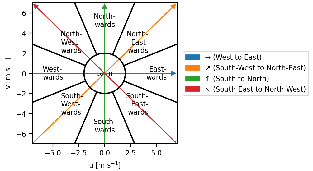
Figure 1 Definition of wind sectors (black) and wind axes (colored) based on wind speed (u, v). Note that “calm” is included in all four wind axes.

For each wind sector separately, the respective TROPOMI pixels are re-gridded on a regular lat–long grid with 0.05° resolution.

3.2 Seasonal means

Emissions could potentially vary over the year. Likewise, the NO_x lifetime is expected to depend on season, in particular due to the impact of the SZA on photochemistry. Thus we perform the following analysis separately for different seasons.

As the NO₂ photolysis rate is driven by the SZA, which shows a seasonality with a minimum and maximum close to the solstices, we define seasons accordingly as winter (NDJ: November, December, January), spring (FMA: February, March, April), summer (MJJ: May, June, July) and autumn (ASO: August, September, October) in this study; i.e., winter and summer comprise measurements of the lowest and highest SZA, respectively, for the Northern Hemisphere.

For each wind sector and each season, the gridded NO_x column densities and the associated wind vectors are averaged separately. The seasonal mean NO_x column density for the different wind sectors is shown exemplarily for Riyadh in winter (Fig. 2) and Paris in summer (Fig. 3). The respective maps for all cities and seasons with a successful fit (see below) are provided in the Supplement.

.

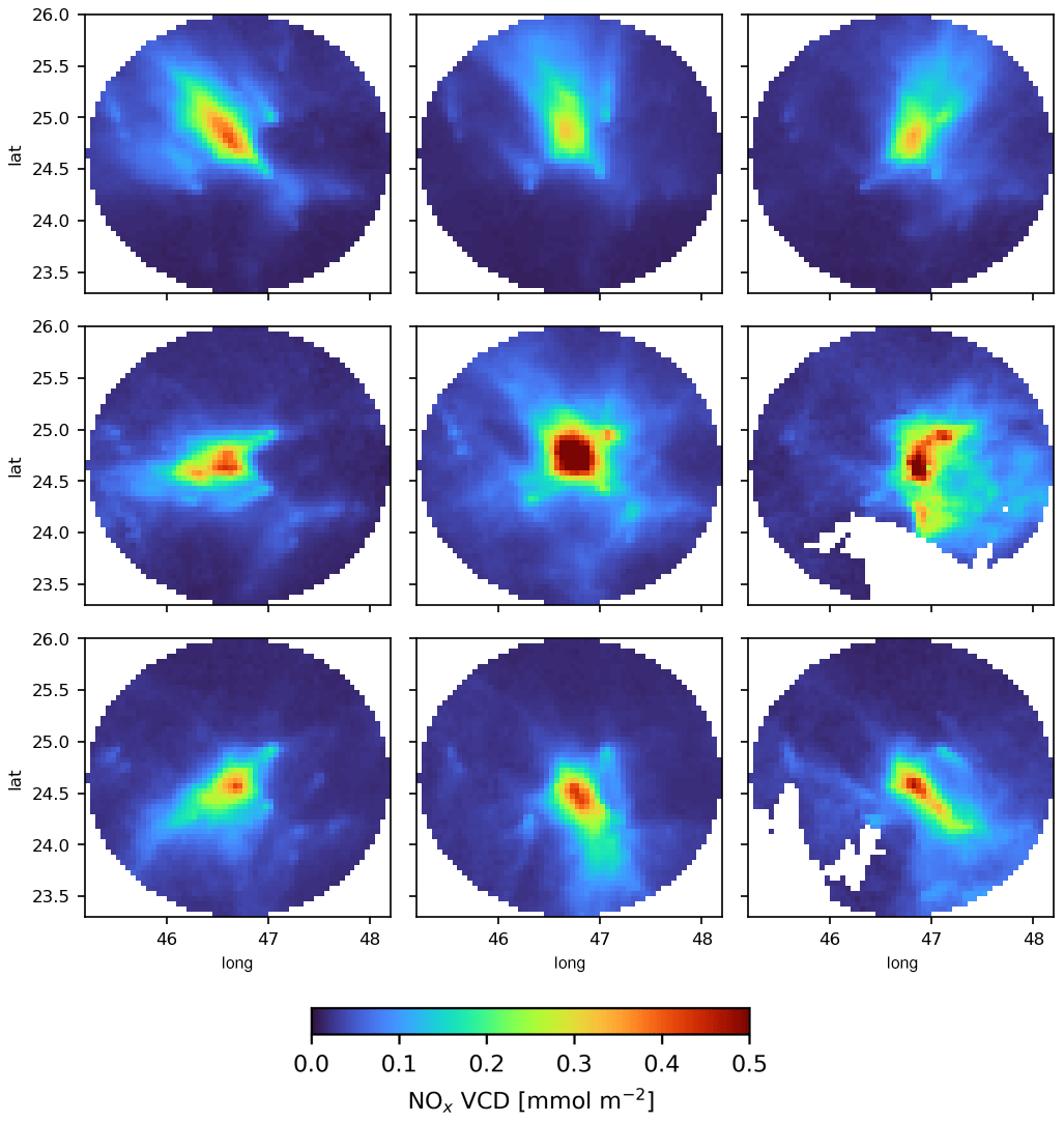
Figure 2 Mean NO_x distribution for Riyadh depending on wind conditions for winter months (NDJ) in the PAL period (May 2018–November 2021). The central panel displays the distribution for calm conditions (w<2 m s⁻¹). The surrounding panels show the respective patterns for the eight different wind sectors as defined in Fig. 1.

.

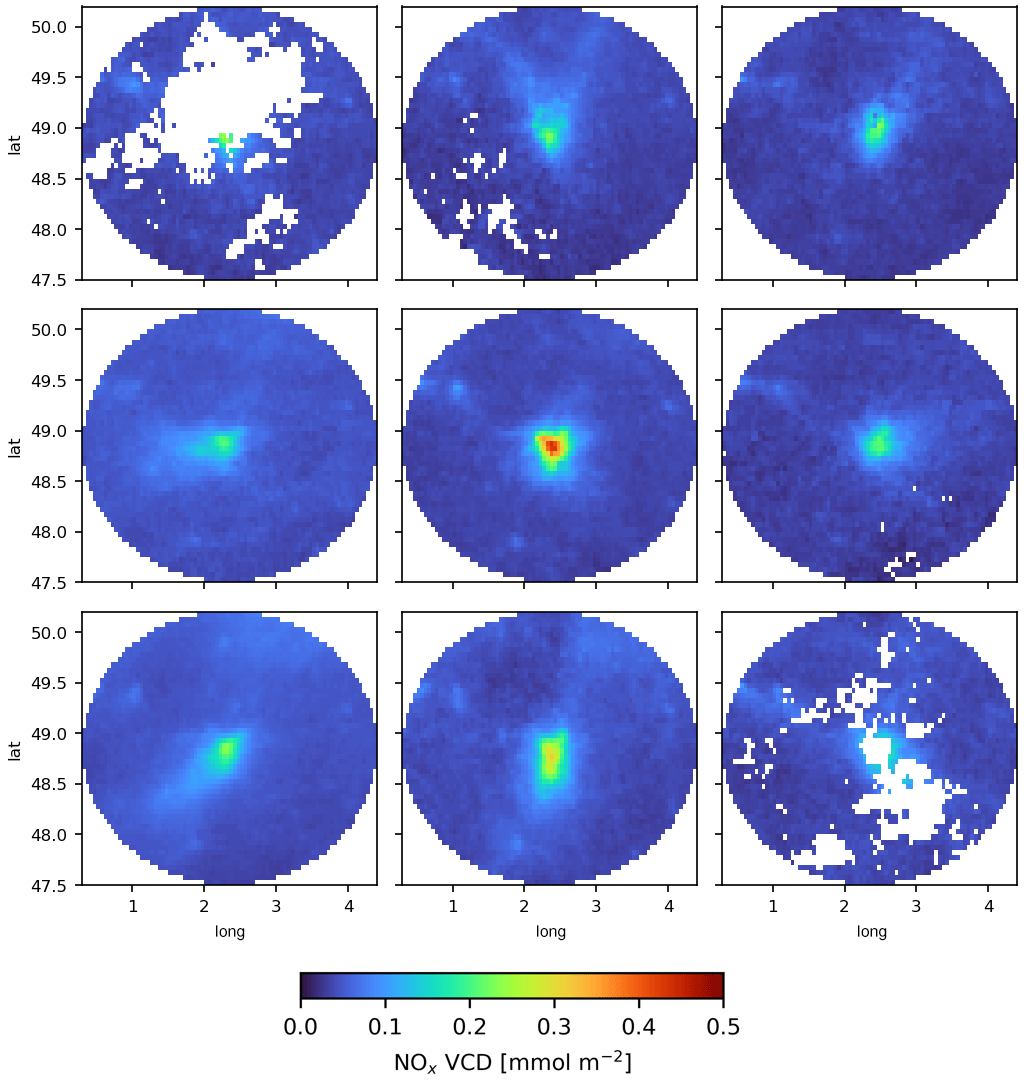
Figure 3 Mean NO_x distribution for Paris depending on wind conditions for summer months (MJJ) in the PAL period (May 2018–November 2021). The central panel displays the distribution for calm conditions (w<2 m s⁻¹). The surrounding panels show the respective patterns for the eight different wind sectors as defined in Fig. 1.

3.3 Considered distances

In this study, we consider two different distances for different purposes.

• For the investigation of the downwind patterns for different wind conditions and the respective fit of the forward model (Sect. 3.5), we consider distances of 145 km upwind and downwind.

• For the quantification of emissions, we consider distances of ± 50 km around the city center, which we consider large enough to actually cover the full extent of the city or conurbation but small enough to limit interference with neighboring cities (which cannot always be avoided). This distance of 50 km is applied for the integration of columns to line densities in the across-wind direction (Sect. 3.4) as well as for the integration of the fitted emission density to total emissions (Sect. 3.5). In other words, the derived emissions refer to a total area of 100 × 100 km².

3.4 Wind axes and line density sets

For each axis (west to east, southwest to northeast, south to north, and southeast to northwest; compare Fig. 1), the mean line density is calculated for calm conditions as well as forward and backward wind direction by integrating the seasonal mean NO_x column density maps in the across-wind direction (± 50 km), yielding the NO_x amount per length unit. Line densities cover the range −145 to 145 km on a 10 km grid, i.e., represent vectors of length 29. Note that the VCD for calm conditions is the same for each axis, but due to the integration in the across-wind direction, the line densities for calm conditions are different for the four axes. The resulting line densities for Riyadh in winter and Paris in summer are displayed in Fig. 4. The respective line densities for all cities and seasons with a successful fit (see below) are provided in the Supplement.

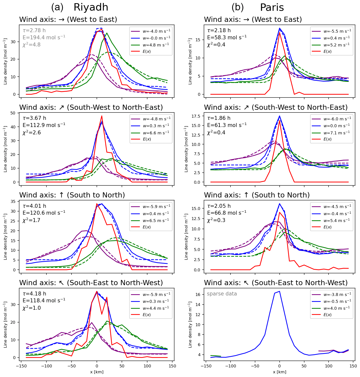
Figure 4 Mean NO_x line densities for (left) Riyadh in winter (NDJ) and (right) Paris in summer (MJJ) depending on wind conditions. The panels show the different wind axes. For each axis, the line densities for calm conditions (blue) and forward (green) and backward (purple) wind directions are displayed as straight lines. If the lifetime and emission fit succeeds, the corresponding fitted line densities are shown as dashed lines, and the fitted emission density is displayed in red. Fitted lifetime and emissions are provided as text in each panel, whereby gray indicates poor fit results which are discarded (see Sect. 3.6).

3.5 Lifetime and emission fit

The lifetime and emission estimates are determined from a nonlinear least-squares inversion (“fit”) that uses the observed patterns of line densities for calm conditions as well as forward and backward winds simultaneously.

The fit is performed for each axis (compare Fig. 1) separately based on the following forward model:

$$\begin{array}{}\text{(1)}& L_i\left(x\right)=E\left(x\right)*\exp \left({\displaystyle \frac{-x}{w_i\cdot \mathit{\tau }}}\right)*\exp \left({\displaystyle \frac{-x^{\mathrm{2}}}{\mathrm{2}{\mathit{\sigma }}^{\mathrm{2}}}}\right)+b_i.\end{array}$$

The index i refers to the three different wind conditions (calm, forward, backward). L_i(x) denotes the line densities, i.e., the columns integrated in the across-wind direction, for calm, forward and backward wind conditions. E(x) represents the spatial density of emissions. It is considered to be the same for all three wind conditions. The symbol “*” indicates mathematical convolution. The first convolution term (to be truncated to x≥0) describes the downwind decay of the emitted NO_x with the e-folding lifetime τ, which is converted to an e-folding distance by multiplication with the mean wind speed w_i. The second convolution represents a simple Gaussian smoothing that accounts for effects like the temporal variation of wind speeds as well as the extent of the TROPOMI ground pixels. σ is fixed to 7 km; different a priori values for σ hardly modify the results. b_i is the respective (wind dependent) NO_x background line density.

Based on the observed line densities within 145 km of the city center, the distribution of emission densities E(x), lifetime τ and backgrounds b_i are fitted simultaneously. In other words, the free parameters (τ, 3 components of b and 29 components of E, in total 33 parameters) are constrained by up to 3 × 29 = 87 components of the measured line densities L_i.

Figure 4 displays the measured (straight) and fitted (dashed) line densities for Riyadh in winter and Paris in summer, respectively. The fitted emission densities E(x) are shown in red. Note that E(x) has the same unit as L(x) (amount per length unit) and corresponds to the hypothetical line density in the case of no wind transport, no background and no smoothing. For real observations, E(x) (red line) is similar to L(x)_calm (blue line) but not identical due to the effects of smoothing, background and calm conditions considering wind speeds up to < 2 m s⁻¹.

The emission rate of the considered hot spot is then derived by spatial integration of E(x) from −50 to +50 km (yielding the total amount of NO_x) divided by τ (yielding emission rates in amount per time unit). Likewise, E(x) is integrated for $x<-\mathrm{50}$ and x>50 km in order to check for and flag potential interfering sources (see next section).

The respective fit results for all cities and seasons with a successful fit are included in the line density plots provided in the Supplement.

3.6 Selection and averaging of fit results

The forward model described above allows us to quantify the emission distribution and total emissions around large cities. However, for robust fit results, a sufficient number of observations is necessary. Thus, a fit is only performed if

• at least two wind conditions have sufficient data (less than 10 % spatial gaps in the seasonal mean column density map), and

• the difference in wind speed is sufficiently large (4 m s⁻¹ between calm and windy conditions – forward or backward – or 8 m s⁻¹ between forward and backward wind) in order to constrain the fit procedure by clearly distinct outflow patterns.

From the 11200 combinations (700 cities, four seasons, four axes), a fit was performed for 2154 cases. These fit results are considered further only if the following holds.

• The reduced χ² of the fit is <3. This is fulfilled for 1862 cases, i.e., in 86 % of all performed fits. This criterion removes fit results of poor performance. For instance, for Riyadh in summer, the observed eastward outflow for westerly winds is not as pronounced as for the other wind directions (Fig. 2), and the respective line densities are not reproduced well by the forward model (green line for the first wind axis for Riyadh in Fig. 4). Due to the enhanced χ² of 4.8, this wind axis is skipped. The reason for the poor match of the fitted line densities is probably that ERA5 wind speeds and/or directions do not match the actual transport well for the observations sorted into the west-to-east direction.

• The fitted lifetime is plausible, i.e., between 1 and 10 h. This selection skips 151 fits with a lifetime that is too low and 34 fits with a lifetime that is too long.

• Interfering emissions (i.e., E(x) integrated for $x<-\mathrm{50}$ or x>50 km) are lower than the city emissions themselves. In the case of interfering emissions, the city is completely removed from the further analysis.

Finally, for each city, the results for the different axes are averaged and weighted by the number of contributing wind conditions for each axis (the more observations, the higher the weight) as well as the fit performance (the lower the χ², the higher the weight). The minimum requirement is that the fit worked for at least one season with either one axis where fit results for all three wind conditions are available or two or more axes where fit results for two wind conditions are available.

With these strict selection criteria, emissions were derived for 100 cities out of the original list of 700 cities with >1 million inhabitants. Note that for most cities, valid emission estimates could only be derived for one or two seasons; in total, 210 lifetime and emission estimates could be made.

4 Results

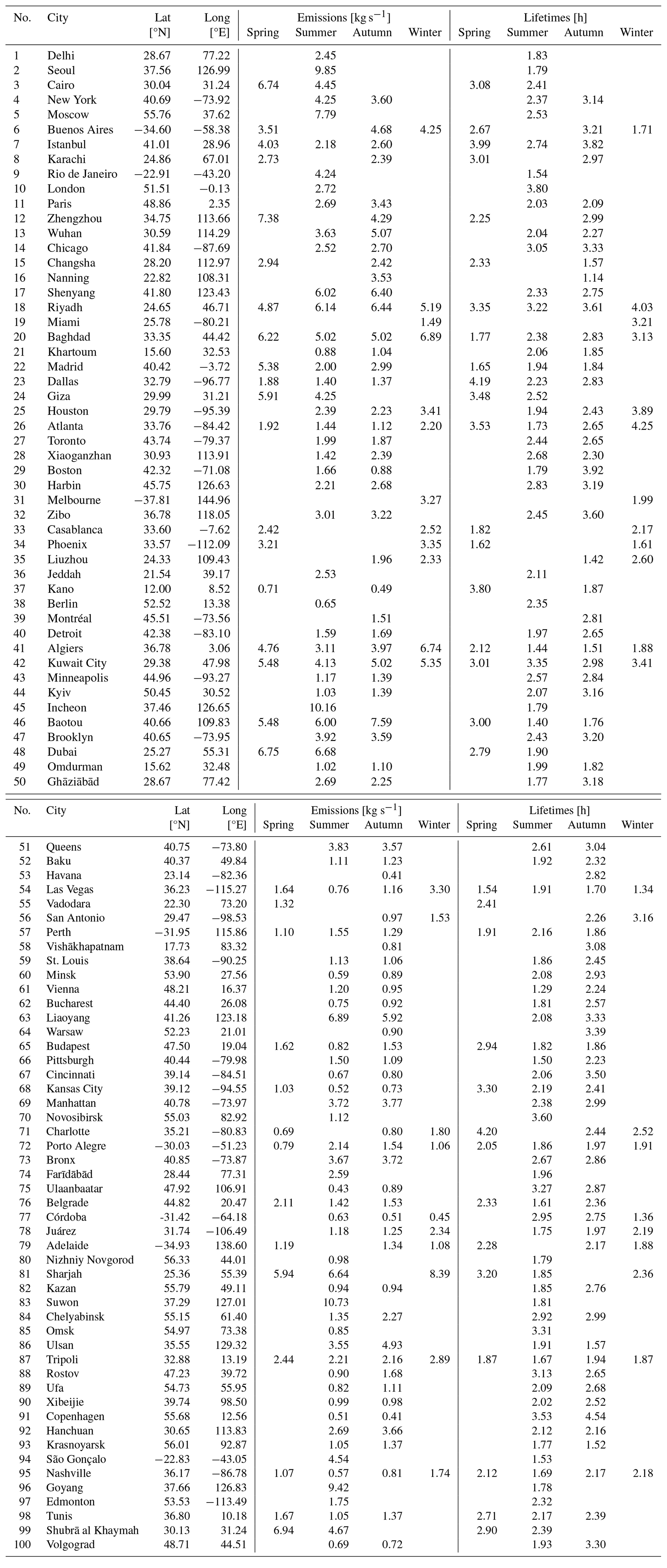
Within this study, seasonal mean NO_x lifetimes and emissions were derived for 100 cities. The results are listed in Table 1. Below we analyze the results for emissions and lifetimes in more detail.

Table 1 Seasonal NO_x emissions and lifetimes for 100 megacities. Seasons are defined as spring (FMA), summer (MJJ), autumn (ASO) and winter (NDJ); for cities in the Southern Hemisphere, the actual meteorological season is flipped.

4.1 Emissions

Figure 5 displays a comparison of the derived seasonal emissions compared to EDGAR (v6.1, integrated over an area of 100 × 100 km² corresponding to the ranges of ± 50 km applied for across-wind integration of VCDs as well as for the integration of emission densities). Overall, the comparison is reasonable; the emissions from both data sources show a correlation of R=0.72. On average, the ratio of TROPOMI to EDGAR is 1.05 (mean of individual ratios) and 0.86 (ratio of means), respectively. However, fluctuations are quite large. The most extreme deviations (labeled by city name in Fig.  5) are discussed in detail in Sect. 5.3.

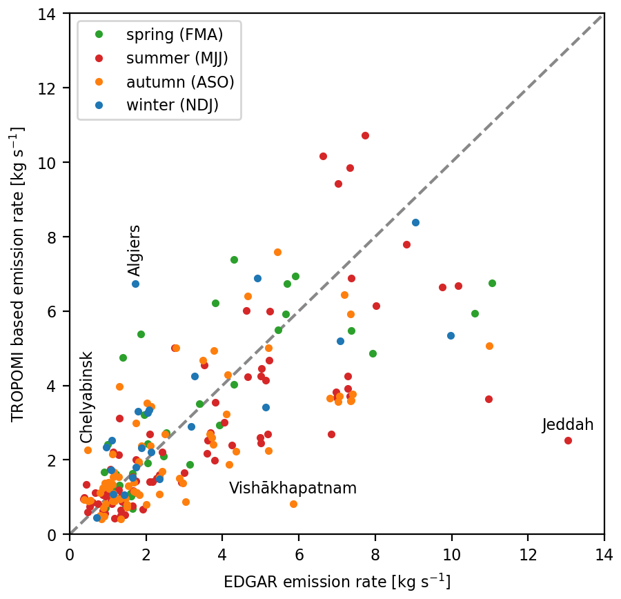
Figure 5 Seasonal NO_x emissions from TROPOMI, averaged over the PAL period of May 2018 to November 2021 (y axis), compared to the respective EDGAR emissions for 2018 (x axis) integrated over an area of 100 × 100 km². Uncertainties for the TROPOMI-based estimates are about 30 %–50 % (Sect. 5.2). City labels indicate cases with the highest and lowest ratios, respectively, which are discussed in more detail in Sect. 5.3.

A combined seasonal analysis (like the mean seasonality of all cities or cities within a latitude range) is not meaningful as there are seasons missing for most cities. Thus we focus on those nine cities where the fit worked for all seasons (Fig. 6). The resulting seasonal cycles differ with respect to amplitude and patterns: while there is low seasonal variety found for Tripoli, emissions are maximal in summer and autumn for Riyadh but minimal for Baghdad. Also, the comparison to EDGAR is rather diverse: patterns are very similar for Baghdad but different for, e.g., Riyadh. For some cities, EDGAR does not show seasonality, but TROPOMI does (Algiers, Las Vegas, Porto Alegre), while for others, the opposite is the case (Kuwait city, Tripoli).

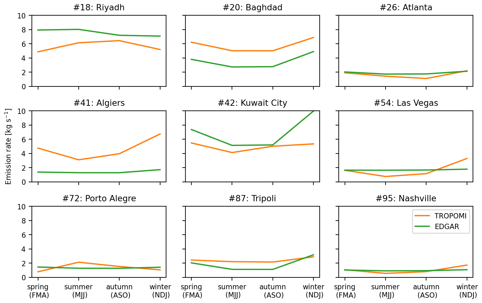
Figure 6 Seasonality of emissions based on TROPOMI estimates (orange) and according to EDGAR (green) for the nine cities where the retrieval yields results for all seasons.

4.2 Lifetimes

The lifetime fit based on Eq. (1) generally yields stable fit results for τ for individual wind axes. Few remaining outliers (below 1 h or above 10 h) have been removed by the selection criteria described in Sect. 3.6.

The resulting weighted mean lifetimes for the considered cities are generally quite short (2.44 h on average) and show only low variability (0.68 h standard deviation). Figure 7 displays (a) a histogram of the fitted lifetimes and (b) the seasonal results (color coded) as a function of latitude. The latter do not reveal a clear pattern of higher lifetimes at higher latitudes or in hemispheric winter (see Sect. 5.4).

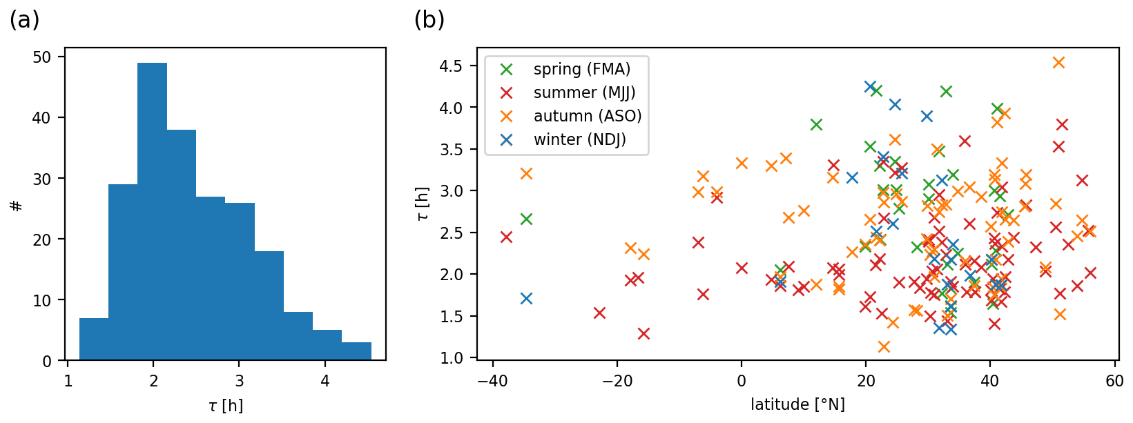
Figure 7 Derived effective lifetimes τ. (a) Histogram of seasonal lifetime results for the 100 investigated cities. (b) Latitudinal dependency of seasonal (color coded) lifetimes. Seasons are defined as winter (NDJ), spring (FMA), summer (MJJ) and autumn (ASO); for cities in the Southern Hemisphere, the actual meteorological season is flipped.

5 Discussion

5.1 Benefits

Satellite measurements of the downwind plume evolution of urban emissions yield model-independent, observation-based constraints of the city emissions and the corresponding effective lifetime. Compared to previous studies, the proposed new method of fitting the downwind patterns of opposing wind directions at the same time has several advantages.

1. Instead of assuming the emissions to be distributed by a Gaussian, possible spatial variations of emissions are explicitly considered.

2. A potential wind dependency of the background is accounted for.

3. The fit is generally well constrained by the spatial patterns for opposite wind directions, resulting in realistic lifetime fits in most cases.

5.2 Errors and limitations

5.2.1 NO₂ columns

For v1 of the TROPOMI NO₂ column densities, a low bias was reported over urban areas (Judd et al., 2020; Lange et al., 2023). In the PAL dataset, based on the NO₂ processor version v2.3.1, many retrieval steps have been improved. In particular, an improved cloud algorithm has been used, resulting in higher cloud altitudes and thus lower air-mass factors and higher NO₂ columns (Eskes et al., 2021; van Geffen et al., 2022). Thus, the reported low bias is expected to be reduced. However, any remaining bias in the NO₂ column would directly affect the presented (as well as any other TROPOMI-based) emission estimate.

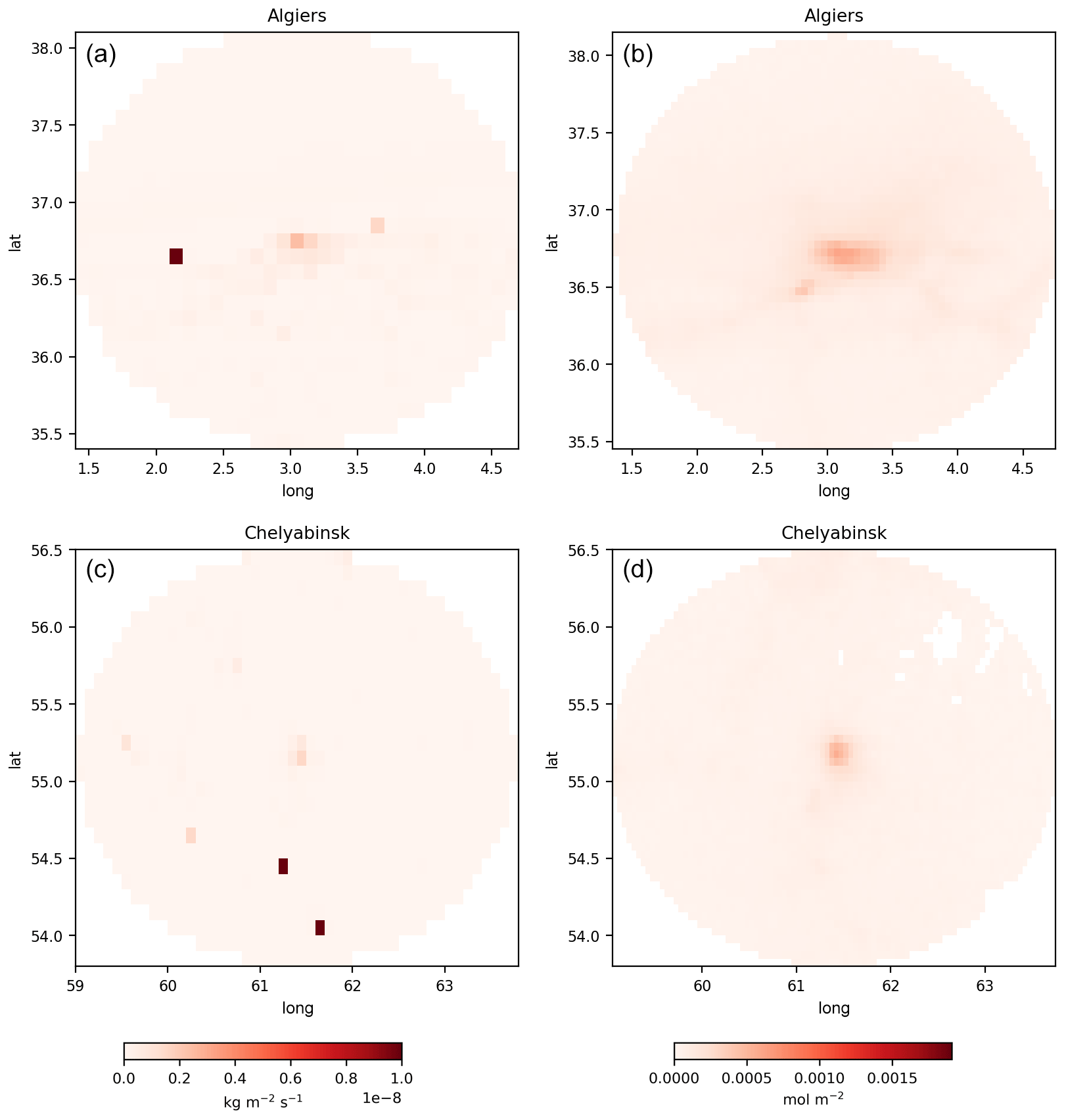
Figure 8 EDGAR NO_x emissions (a, c) and TROPOMI NO_x VCDs for calm wind conditions (b, d) around Algiers (no. 41) in winter (a, b) and Chelyabinsk (no. 84) in autumn (c, d). The color bar for VCDs corresponds to the emission color bar for mass conservation with a lifetime of 2.44 h.

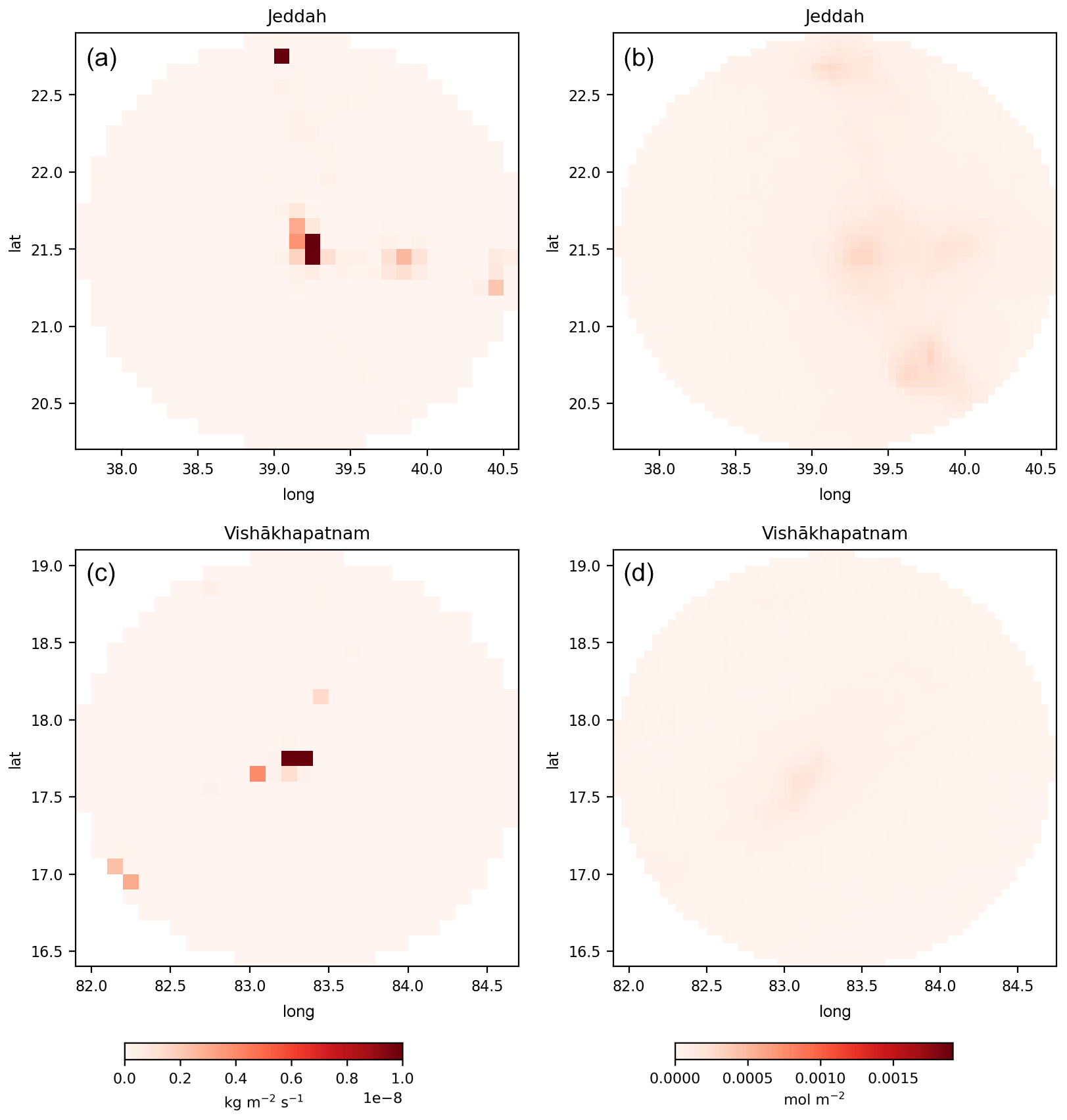
Figure 9 EDGAR NO_x emissions (a, c) and TROPOMI NO_x VCDs for calm wind conditions (b, d) around Jeddah (no. 36) in summer (a, b) and Vishākhapatnam (no. 58) in autumn (c, d). The color bar for VCDs corresponds to the emission color bar for mass conservation with a lifetime of 2.44 h.

5.2.2 Wind fields

In this study, we use ERA5 wind fields, which have been stored on a 1° grid and at 6 h intervals in order to reduce data amount at the cost of wind field accuracy. We are currently preparing the implementation of high-resolution ERA5 wind data with hourly sampling on a 0.25° latitude–longitude grid for future studies. So far, we have applied high-resolution wind data for the calculation of the advection of SO₂ fluxes (Jost et al., 2024) based on the algorithm developed for NO_x (Beirle et al., 2023). On average, emission estimates for high-resolution wind fields were found to be higher by about 5 %. Such a systematic effect is expected, since any error in wind direction Δα, random or systematic, causes an underestimation of the wind component in the actual wind direction and thus an overestimation of lifetimes and an underestimation of emissions (see the Supplement of Beirle et al., 2019).

But even with high-resolution wind fields, the simplified description of horizontal transport of the whole tropospheric column by one horizontal wind field (here: interpolated at 500 m a.g.l.) remains a significant source of uncertainty for this and similar methods. As discussed in Beirle et al. (2011), uncertainties of emissions due to uncertainties in wind fields are about up to 30 %.

5.2.3 Lifetime and emission fit

Within the nonlinear least-squares optimization applied to Eq. (1), the best-matching parameters are determined, including their uncertainties. As the new approach of simultaneously fitting patterns for forward, backward and calm wind conditions is strongly constrained, results are generally robust, and the nominal uncertainties resulting from the least-squares inversion are generally low (down to a few percent) and negligible compared to other uncertainties. Thus, the fit errors are not listed.

More realistic uncertainties could in principle be estimated from the standard deviation of fit results among different wind axes. For the example of Riyadh shown in Fig. 4, this would yield 24 % uncertainty for emission rates and 15 % for lifetimes. Note, however, that the “outlier” for wind axis “→” is not considered in the reported mean emissions for Riyadh due to the high χ² value. As there are often only one or two axes available for most cities, this procedure cannot be used for calculating a standard deviation for all cities. But since observation conditions are close to optimal for Riyadh (high albedo, few clouds), higher uncertainties have to be expected for other cities.

One reason for this rather large uncertainty of the fit results – despite the strong constraint from downwind patterns in opposite directions – is probably the assumption of steady state (over distances up to 145 km downwind), while in reality, emissions, wind fields and chemistry change over time.

Overall, we roughly estimate the total uncertainty (including wind) of the estimated emissions as typically 30 % up to 50 %.

5.3 Emissions

There are some aspects that have to be kept in mind when interpreting the derived emissions and the comparison to EDGAR.

• The given emission rates are meant to represent the integrated emissions within ± 50 km from city center in both directions, corresponding to the chosen across-wind range used for calculating line densities and the integration range of the fitted emission density E(x).

  This implies that the emissions from large cities close to each other interfere and are counted for each city repeatedly (for the TROPOMI estimate as well as for the estimated EDGAR value). This happens, for instance, for the large cities around Seoul, i.e., Incheon, Suwon and Goyang, which are all listed with emission rates close to 10 kg s⁻¹. These values must not be added.

• EDGAR emissions are provided for the year 2018, while the TROPOMI estimate is derived for the time range covered by PAL (May 2018 – November 2021). Thus, deviations have to be expected in the case of recent changes in emissions. This is particularly the case for the massive lockdowns in 2020 and 2021.

For these reasons and due to the estimated uncertainty of up to 50 % (see Sect. 5.2), no perfect agreement can be expected. Actually, for most cities and seasons, the TROPOMI-based estimates agree with EDGAR within the given uncertainties. However, for some cities, large deviations have been observed which exceed the estimated uncertainty by far.

• TROPOMI-based emissions for Algiers (no. 41) in winter and Chelyabinsk (no. 84) in autumn are higher than EDGAR emissions by a factor of 3.9 and 4.9, respectively. Figure 8 displays the spatial distribution of NO_x emissions according to EDGAR around these cities compared to the observed NO_x pattern for calm wind conditions. In both cases, EDGAR emissions within the city are very low, but additional sources show up in the EDGAR emissions west of Algiers (Hadjret en Nouss power plant) and south of Chelyabinsk (Yuzhnouralskaya and Troitskaya power plants). The TROPOMI VCD, however, does not show indications for strong point sources at these locations¹. For Algiers, emission estimates were derived for all seasons (Fig. 6), with winter emissions found to be more than double summer emissions. In contrast, EDGAR emissions hardly show any seasonality. But for all seasons, TROPOMI-based estimates are significantly higher than EDGAR.

• For Jeddah (no. 36) in summer and Vishākhapatnam (no. 58) in autumn, EDGAR emissions are higher than the TROPOMI-based estimate by a factor of 5.2 and 7.2, respectively. Mean TROPOMI NO_x VCDs are far lower than would be expected for the given EDGAR emissions (Fig. 9).

For all of these cities, the lifetime and emission fits work properly (see Supplement), and the fitted lifetimes are well within the typical range found for other cities (Table 1). Thus we conclude that our comparison actually hints to EDGAR emissions that are too low or too high, which should be checked for these cities.

5.4 Lifetimes

The effective NO_x lifetime has been found to be rather short (a few hours, 2.44 h on average) with only weak variability (0.68 h SD). These values are generally consistent with low NO_x lifetimes reported in previous studies (de Foy et al., 2014; Laughner and Cohen, 2019; Lorente et al., 2019; Laughner and Cohen, 2019; Lange et al., 2022).

In contrast to Lange et al. (2022), however, we do not find a clear increase in lifetime with latitude or a clear seasonal dependency. This should be investigated further but is probably – at least partly – related to the strict SZA < 65° criterion applied in this study, resulting in the removal of wintertime measurements at middle and high latitudes. Thus, larger lifetimes in winter would be probably observed with this method as well if larger SZA were included.

6 Conclusions

We present a new method for the estimation of urban emissions of NO_x and the corresponding effective lifetime of NO_x. Compared to previous methods of fitting an EMG to the downwind plume (intrinsically assuming a “point source”), we invert the downwind patterns of opposing wind directions simultaneously. This approach has two major advantages: (1) the spatial distribution of emission sources within a city can be resolved, and (2) the fit is generally well constrained. The main disadvantage is that the method requires temporal mean patterns for opposing wind directions and thus only works on long-term temporal averages.

Within ESA's World Emission project, the method was successfully applied to 100 cities worldwide. The derived emissions show reasonable agreement with EDGAR emissions (R=0.72, ratio of means 0.86). The cities with the largest deviations have been checked in more detail and hint to a low or high bias of EDGAR emissions for these cities.

Lifetimes were found to be 2.44 ± 0.68 h on average. No clear seasonal or latitudinal dependency was found, but this might be due to the removal of observations with large SZA (>65°).

The remaining uncertainties and the partly inconsistent results for different wind axes have to be considered in relation to the assumptions made:

• the assumption of steady state (within 145 km downwind of the city center),

• the representation of the complex and nonlinear NO_x chemistry by one single first-order loss time constant, and

• the simplified representation of transport by horizontal wind fields, ignoring 3D effects and different wind fields at different altitudes of the column.

These assumptions cause intrinsic uncertainties of the presented (as well as other similar) methods, which probably cannot simply be removed just by improved algorithms.