Using a portable FTIR spectrometer to evaluate the consistency of Total Carbon Column Observing Network (TCCON) measurements on a global scale: the Collaborative Carbon Column Observing Network (COCCON) travel standard

To fight climate change, it is crucial to have a precise knowledge of greenhouse gas (GHG) concentrations in the atmosphere and to monitor sources and sinks of GHGs. On global scales, satellites are an appropriate monitoring tool. For the validation of the satellite measurements and to tie them to the World Meteorological Organization (WMO) trace gas scale, ground-based Fourier transform infrared (FTIR) networks are used, which provide reference data. To ensure the highest-quality validation data, the network must be scaled to the WMO trace gas scale and have a very small site-to-site bias. Currently, the Total Carbon Column Observing Network (TCCON) is the de facto standard FTIR network for providing reference data. Ensuring a small site-to-site bias is a major challenge for the TCCON. In this work, we describe the development and application of a new method to evaluate the site-to-site bias by using a remotely controlled portable FTIR spectrometer as a travel standard (TS) for evaluating the consistency of columnar GHG measurements performed at different TCCON stations, and we describe campaign results for the TCCON sites in Tsukuba (Japan), East Trout Lake (Canada) and Wollongong (Australia). The TS is based on a characterized portable EM27/SUN FTIR spectrometer equipped with an accurate pressure sensor which is operated in an automated enclosure. The EM27/SUN is the standard instrument of the Collaborative Carbon Column Observing Network (COCCON). The COCCON is designed such that all spectrometers are referenced to a common reference unit located in Karlsruhe, Germany. To evaluate the long-term stability of the TS instrument, it is placed side-by-side with the TCCON instrument in Karlsruhe (KA) and the COCCON reference unit (the EM27/SUN spectrometer SN37, which is operated permanently next to the TCCON-KA site) between deployments to collect comparing measurements.

At each of the visited TCCON sites, the TCCON spectrometers collected low-resolution (LR) (0.5 cm⁻¹) and high-resolution (HR) (0.02 cm⁻¹) measurements in an alternating manner. Based on the TS as a portable standard, the measurements are compared to the Karlsruhe site as a common reference. For Tsukuba and Wollongong, the agreement with the reference in Karlsruhe found for XCO₂ is on the 0.1 % level for both the LR and HR measurements. For XCH₄, the agreement is at the 0.2 % level, with the low-resolution measurements showing a low bias at both sites and for both gases. For XCO, the deviations are up to 7 %. The reason for this is likely to be a known issue with the CO a priori profiles used by the TCCON over source regions. In East Trout Lake (ETL), the TCCON spectrometer broke down while the TS was en route to the station. Hence, no side-by-side comparison was possible there.

An important auxiliary value for FTIR retrievals is the surface pressure. Using the pressure sensor in the TS, the surface pressure measurements at each site are also compared. The surface pressure analysis reveals excellent agreement (0.027, 0.135 and 0.094 hPa) for the Tsukuba, ETL and Wollongong sites.

1 Introduction

According to the sixth report of the Intergovernmental Panel on Climate Change (IPCC), there is overwhelming evidence concerning the human influence on the warming of the earth's atmosphere (Allan et al., 2021) caused by the release of greenhouse gases (GHGs) into the atmosphere. Specifically, increasing atmospheric concentrations of CO₂ and CH₄ are the main drivers of global warming. Hence, it is of utmost importance to have a precise knowledge of the GHG concentrations in the atmosphere to better quantify anthropogenic and natural sources and sinks and thus the carbon cycle. Highly accurate in situ measurements of GHGs are performed by the Integrated Carbon Observation System (ICOS) network in Europe (ICOS RI et al., 2022) and by NOAA provided in the ObsPack framework (Cox et al., 2022). In situ measurements provide high accuracy and precision. However, they cannot directly be compared to satellite data, as satellites provide column-averaged GHG concentrations, and the in situ measurements are provided at distinct, single heights and lack representativeness on the scale of the satellite observations. This gap can be closed by Fourier transform infrared (FTIR) networks which also collect column-averaged data and can be tied to the high quality in situ measurements.

The Total Carbon Column Observing Network (TCCON) (Wunch et al., 2011a) is a collaboration of 28 (status in March 2023) FTIR spectrometer sites measuring total columns of GHGs worldwide. The final product of the TCCON are column-averaged dry-air mole fractions (denoted as XGas in the following) of various GHGs and other trace gases which are calculated by

$$\begin{array}{}\text{(1)}& X\mathrm{Gas}={\displaystyle \frac{{\text{VC}}_{\mathrm{gas}}}{{\text{VC}}_{{\mathrm{O}}_{\mathrm{2}}}}}\cdot \mathrm{0.2095}.\end{array}$$

Here, VC${}_{{\mathrm{O}}_{\mathrm{2}}}$ is the vertical column number of molecules per square centimeter of O₂ and VC_gas the vertical column amount of the corresponding gas.

In this work, we focus on XCO₂, XCH₄ and XCO. The official evaluation software of TCCON is called GGG, its latest version is GGG2020. For current TCCON data generated with GGG2020, the estimated error budget is 0.12 % (0.47 ppm) for XCO₂, 0.22 % (3.90 ppb) for XCH₄ and 1.7 % (1.70 ppb) for XCO (column “Budged” of Table 5 in Laughner et al., 2024). The absolute concentrations used to convert between absolute and relative errors are 400 ppm for XCO₂, 1800 ppb for XCH₄ and 100 ppb for XCO.

The site-to-site consistency for TCCON data generated with GGG2020 has been evaluated by Laughner et al. (2024) (column “MAD” of Table 5). The biases are 0.11 % (0.42 ppm) for XCO₂, 0.27 % (4.9 ppb) for XCH₄ and 8.1 % (8.1 ppb) for XCO. The numbers are calculated from the spread of the TCCON versus in situ airplane profiles.

In the past, the data measured by the TCCON were successfully used for satellite validation (Sha et al., 2021; Hong et al., 2022; Wu et al., 2018; Wunch et al., 2017; Yoshida et al., 2013; Wunch et al., 2011b; Dils et al., 2014) and for scientific studies like correlating the CO₂ concentrations in the Northern Hemisphere with the temperature (Wunch et al., 2013) or for evaluating the biosphere exchange (Messerschmidt et al., 2013).

To produce reliable reference data, two things have to be considered. The first item is to ensure that the network as a whole is accurately tied to the World Meteorological Organization's (WMO's) trace gas scale (Hall et al., 2021; Dlugokencky et al., 2005). The second is to minimize the station-to-station biases across the network due to the non-nominal behavior of the spectrometer. Currently, this connection to the WMO trace gas scale is achieved by vertically integrating colocated airborne profile observations or via a new technique called AirCore (Karion et al., 2010) to compare with the TCCON results (Wunch et al., 2010; Messerschmidt et al., 2011; Sha et al., 2020a). In short, AirCore profiles are derived by mounting a long, evacuated tube on a balloon or aircraft. During descent, the tube gets filled. Height-resolved profiles of GHG concentrations can be derived from the record.

In addition to the in situ comparisons, the TCCON quality assurance (QA) has two supplementary methods: the monitoring of the instrumental line shape (ILS) and the evaluation of XAIR (also called XLUFT). They are explained in detail in Sect. 2.1. However, while both the ILS analysis and the XAIR evaluation are very useful methods for detecting deviations from the expected instrumental characteristics at individual sites, they cannot guarantee that the final XGas products will be consistent within the network.

In this work, an additional method of further enhancing the TCCON's quality management is presented and applied. It is based on a portable EM27/SUN FTIR spectrometer operated in the framework of the Collaborative Carbon Column Observing Network (COCCON) (Frey et al., 2019), which will be used as a traveling standard. This activity aims directly at the improvement of the site-to-site consistency. The EM27/SUN spectrometer is a low-resolution, portable FTIR spectrometer. The prototype was developed by the Karlsruhe Institute of Technology (KIT) in cooperation with Bruker starting in 2011 (Gisi et al., 2012) and became available as a commercial item in 2014. In 2015 an extension of the original configuration was implemented by adding a second detector covering the 4000–5000 cm⁻¹ spectral range (Hase et al., 2016). This additional channel allows for retrieving XCO and an alternative XCH₄ product, which we refer to as ${\mathrm{XCH}}_{\mathrm{4}}^{\mathrm{S}\mathrm{5}\mathrm{P}}$, as the same spectral region is measured to retrieve CH₄ by the spaceborne TROPOMI (TROPOspheric Monitoring Instrument ) spectrometer aboard the Sentinel-5P (S5P) satellite.

The EM27/SUN spectrometer has proven its high level of instrumental stability in various city campaigns (Tu et al., 2022; Alberti et al., 2022b; Hase et al., 2015; Dietrich et al., 2021; Chen et al., 2016) and long-term studies (Alberti et al., 2022a). It has even been successfully deployed on ships (Klappenbach et al., 2015; Butz et al., 2022) and on cars (Butz et al., 2017; Luther et al., 2019).

Due to the stable instrumental characteristics it is meaningful to perform side-by-side comparisons of EM27/SUN spectrometers to quantify residual instrument-specific imperfections in the framework of campaign deployments. Moreover, this finding enables the COCCON to evaluate all EM27/SUN FTIR spectrometers before the first deployment, thereby connecting all spectrometers to a common reference (Alberti et al., 2022a; Frey et al., 2019).

Local campaigns for comparing subsets of TCCON sites have been performed using EM27/SUN spectrometers (Mostafavi Pak et al., 2023; Hedelius et al., 2016). Here we present the commissioning and the first results achieved with a dedicated travel standard (TS) unit for systematically evaluating the station-to-station consistency of the TCCON on a intercontinental scale.

Karlsruhe is chosen as the home base of the TS. This is the natural choice as in Karlsruhe there is a TCCON site as well as the EM27/SUN reference spectrometer for the whole COCCON network. Hence, the TS is calibrated against the COCCON reference and the Karlsruhe TCCON site.

Physically, the TS is an EM27/SUN spectrometer housed in an enclosure enabling autonomous operation (Heinle and Chen, 2018; Dietrich et al., 2021). The unit is equipped with a high accuracy pressure sensor (Vaisala PTB330; Vaisala, 2023). Using side-by-side measurements of the TCCON spectrometers with the TS enables us to compare the TCCON spectrometers to the TS as a common reference and hence to compare the XGas results.

For this, it is important to note that the TS is a low-resolution spectrometer and that XGas results derived from spectra recorded side-by-side with different spectral resolutions can differ due to various causes. This is examined in Petri et al. (2012) and also described in Sect. 2.2.2.

To avoid the resulting uncertainties connected to differing resolution, additional low-resolution double-sided interferograms are recorded with the TCCON spectrometer, and these are used in addition to the high-resolution TCCON measurements for the side-by-side comparison. Note that, due to the lower resolution of the TS, its interferograms are lacking the high-resolution section of the interferograms recorded by the TCCON instruments. Therefore, it is not possible to fully evaluate the performance of a TCCON spectrometer by comparison with the TS. However, the gas cell measurements performed by the TCCON cover this missing aspect of verifying the high-resolution part of the TCCON interferogram by providing a characterization of the ILS. A more detailed description of the procedures for measuring station-to-station consistency is provided in the following sections.

The paper is structured as follows: after this introductory section, Sect. 2 introduces the idea and the design choices as well as the practical realization of the TS. Section 3 describes the procedure for monitoring the TS spectrometer by laboratory and side-by-side reference measurements performed at KIT between the campaigns. In Sects. 4 to 6, the data resulting from the observations collected with the TS and the TCCON station spectrometer in Japan, Canada and Australia are presented. Section 7 presents quantitative comparisons between the visited sites and the COCCON reference spectrometer operated in Karlsruhe. Section 8 gives a summary and an outlook.

2 The travel standard: idea and realization

2.1 Idea and description of the travel standard

The creation of a TS originates from the desire to detect potential station-to-station biases across the TCCON on a global scale. The most direct approach to solve this would be to collect side-by-side measurements of the FTIR spectrometers in the TCCON. Unfortunately, the spectrometer used by the TCCON are large, heavy and sensitive, so shipping them around is challenging. More importantly, the instrumental characteristics of the IFS125HR spectrometer, used as the standard TCCON spectrometer, cannot be kept stable during transportation, as a partial dismounting of the interferometer is required for safe transport and variable loads occurring during transport disturb the previous alignment state.

In the past, side-by-side measurements with different TCCON spectrometers have been attempted by several investigators, and these encounters were very useful for gaining insights which helped to further improve the performance of TCCON (Pollard et al., 2021; Messerschmidt et al., 2010). While these studies demonstrated the typical level of consistency achievable in practice with IFS125HR spectrometers, they do not provide an actual side-by-side check of two TCCON sites.

Instead, there are several network-wide consistency checks as outlined in the Introduction:

• comparison with height-resolved in situ data collected by airplanes and AirCore samplers,

• evaluation of the ILS,

• evaluation of XAIR.

In the following, these methods are described in more detail than in the Introduction, and their limitations are discussed. Further technical quantities which are side results of the spectral fits (as, e.g., abscissa wavenumber scale or stretch of the solar absorption lines contained in the spectrum) are also used for QA/QC of the TCCON data products but are not discussed further.

Comparison with in situ data. So far, the TCCON has used in situ measurements collected by airplanes or balloon-based AirCore samplers to assess site-to-site consistency, and they tie the TCCON measurements to the WMO trace gas standard scale (Wunch et al., 2010; Messerschmidt et al., 2011; Karion et al., 2010; Sha et al., 2020a).

However, those measurements are sparse, infrequent and difficult to conduct in highly populated areas with dense air traffic. Nevertheless, they are important for tying TCCON as a whole to the WMO scale, and they can contribute to the performance assessment of individual sites.

ILS evaluation. The use of a gas cell for evaluation of the ILS was implemented for the Infrared Working Group (IRWG) of the Network for the Detection of Atmospheric Composition Change (NDACC) in the 1990s; for details, see Hase et al. (1999). The cell is filled with a known amount of a target gas at low pressure, and the ILS is deduced from the comparison of a measured spectrum with a simulated spectrum using the known cell characteristics (length, pressure, temperature).

The measurements offer high sensitivity for detecting deviations of the spectrometer's modulation efficiency as a function of the optical path difference (OPD) from nominal behavior. The procedure essentially ensures that the shape of spectral lines in the measured atmospheric spectra is reproduced properly.

This procedure, however, covers only a limited spectral range where the cell gas offers useful spectral signatures. Low-pressure gas cells mainly provide a check of the ILS for a high-resolution spectrometer. To verify the modulation efficiency near the zero path difference, which is relevant for the quantification of tropospheric species, additional cells containing gas mixtures at higher pressure would be useful (Hase, 2012). But the preparation and use of different cells is laborious and has not yet been implemented in the operational procedures of the TCCON or the NDACC FTIR networks. Moreover, it is less sensitive for detecting minor disturbances of the low-resolution part of the spectrum (at low OPDs) or for validating the zero level baseline of the recorded atmospheric spectra. Such disturbances critically affect the measured line area and thereby the derived column-averaged GHG concentrations.

XAIR calculations. XAIR is a parameter calculated by the retrieval algorithms to check for consistency. In GGG it is implemented as the following (Wunch et al., 2015):

$$\begin{array}{}\text{(2)}& {\displaystyle }\text{XAIR}={\displaystyle \frac{{\text{VC}}_{\mathrm{air}}}{{\text{VC}}_{{\mathrm{O}}_{\mathrm{2}}}}}\cdot \mathrm{0.2095}-{\mathrm{XH}}_{\mathrm{2}}\mathrm{O}\cdot {\displaystyle \frac{m_{{\mathrm{H}}_{\mathrm{2}}\mathrm{O}}}{m_{\mathrm{dry}\text{-}\mathrm{air}}}},\text{(3)}& {\displaystyle }{\text{VC}}_{\mathrm{air}}={\displaystyle \frac{p_{\mathrm{s}}}{\stackrel{\mathrm{‾}}{g}\cdot \frac{m_{\mathrm{dry}\text{-}\mathrm{air}}}{N_{\mathrm{A}}}}}.\end{array}$$

Here, ${\text{VC}}_{{\mathrm{O}}_{\mathrm{2}}}$ is the total number of O₂ molecules in the air column (in cm⁻²); XH₂O the column-averaged, dry air mole fraction (in parts/parts) of H₂O; $m_{{\mathrm{H}}_{\mathrm{2}}\mathrm{O}}$ (18.02 g mol⁻¹) and m_dry-air (28.964 g mol⁻¹) are the mean molar masses of H₂O and dry air, respectively; N_A is Avogadro's constant (6.022×10²³ molec. mol⁻¹); and $\stackrel{\mathrm{‾}}{g}$ is the column-averaged gravitational constant (in m s⁻²). Note that the gravitation depends on the latitude and therefore cannot be given here. The first part in Eq. (2) compares the total column of dry air (VC${}_{\mathrm{dry}\text{-}\mathrm{air}}=\frac{{\text{VC}}_{{\mathrm{O}}_{\mathrm{2}}}}{\mathrm{0.2095}}$) to the amount of air molecules calculated by using the surface pressure and assuming a hydrostatically balanced atmosphere. The surface pressure, however, depends on the amount of water vapor in the atmosphere. This is considered in the second term. As a technical quantity, it is created to deliver a value near unity for a spectrometer correctly set up and aligned. According to Laughner et al. (2024) for the TCCON, the expected value is 0.999 due to imperfections in the O₂ spectroscopy.

Deviations from this expected value indicate an error with the instrument. Known causes are a bad instrumental line shape (ILS); nonlinearity at the detector; sampling ghosts; and errors in the used surface pressure measurement, in the spectroscopic measurement, or in the estimation of air mass (e.g., line of sight not properly centered on solar disk, undetected time offset). In this work, the data are also evaluated with PROFFAST2, which is the official retrieval software of the COCCON community (Hase et al., 2023; Feld et al., 2023). It is developed at KIT and is explicitly designed to be used with EM27/SUN spectrometers; however, it is also able to handle measurements of several other FTIR low-resolution instruments. When comparing XAIR values of GGG and PROFFAST, it is important to note that the implementation in both packages is inverse to each other. Consequently, when in this paper XAIR of PROFFAST and GGG are compared to each other, the value calculated by PROFFAST is inverted. To make this clear, we add the subscript “GGG” to the XAIR labels to indicate that we are using the standard GGG XAIR values and the inverted PROFFAST XAIR values.

However, both the cell measurements and the XAIR methods do not explicitly validate the final XGas products. Hence, it is not possible to guarantee the compatibility of XGas datasets collected by different stations based on the cell methods and the XAIR quantity.

In summary, we are convinced that the COCCON-TS for the TCCON presented in this paper is a valuable complement to the methods presented above: the TS uses the same measurement principle as the TCCON, and the retrieved XGas values can be compared directly to each other. The TS is easily transportable and is independent of potential overflight restrictions affecting airplane or AirCore measurements. In addition, it is a reasonably inexpensive activity as the measurements can be collected remotely, assuming support of the local TCCON staff. The costs are dominated by shipping. A practical limitation is that temporary import of the TS into countries not recognizing the ATA carnet (the possibility of tax- and duty-free temporary import and export of scientific goods) agreement is more difficult to achieve.

2.2 Shelter hardware and standardized procedure

2.2.1 Shelter hardware

For a TS based on an EM27/SUN spectrometer, there are two key demands. The first is that it needs some kind of enclosure which helps to make the field deployment at the various sites simple and controllable remotely. As it protects the EM27/SUN from precipitation, it is not necessary to deploy it manually for each measurement day which helps to collect more observations. The second is that the hardware should help to maintain temperature and humidity inside the shelter within a range that allows the spectrometer to operate under a wide range of ambient conditions. This is realized by using an enclosure which was developed by Technische Universität München (TU Munich) (Heinle and Chen, 2018; Dietrich et al., 2021). It is equipped with an easy-to-use and reliable software running on a programmable logic controller to control the measurement dome and an internal computer to control the EM27/SUN spectrometer. Figure 1 shows the enclosure including the rotatable dome. Remote access is provided by a router which can connect to the internet via LAN, Wi-Fi or even cellular data. To provide stable temperature and humidity conditions, the enclosure is equipped with a heater and a fan to heat and cool the inside of the enclosure depending on ambient conditions. The temperature is kept above 25 °C to prevent condensation. On a hot summers day, the maximal temperature measured was 40 °C, which is in a range the EM27/SUN spectrometer operates without problems. A rain sensor is mounted to the cover which, in case of rain, induces a rapid closing of the dome to protect the EM27/SUN spectrometer. A small UPS (uninterruptible power supply) is included to close the dome in case of a blackout to not leave the spectrometer unprotected.

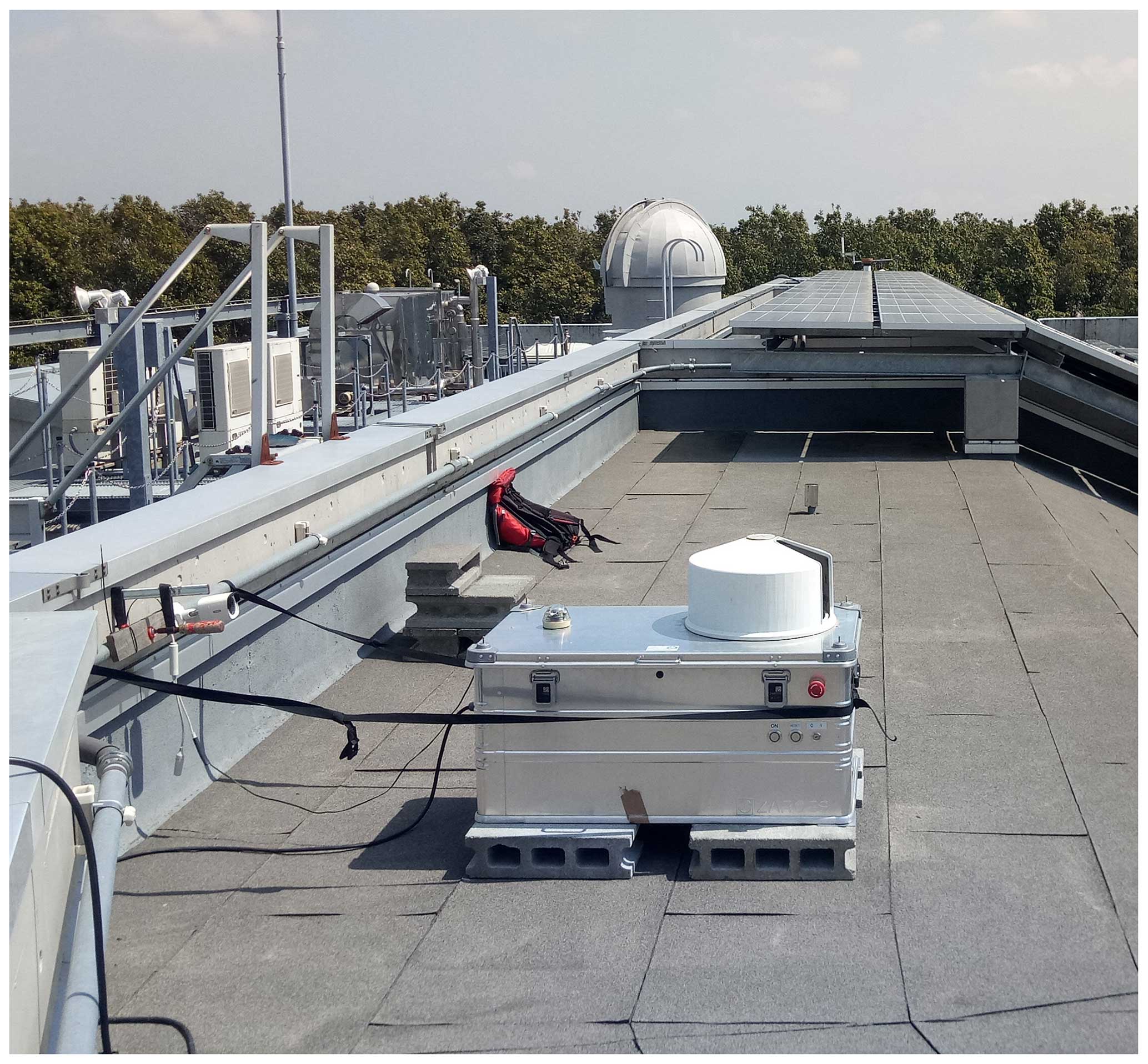
Figure 1 The figure shows the TS in Tsukuba, Japan whilst measuring. The enclosure including its measurement dome, developed by TU Munich, can be seen in the foreground. The white hemisphere in the background is the TCCON dome.

Since the enclosure was primarily designed to be used in Europe, it was in its original configuration not able to deal with power grids other than the European one. Hence, the enclosure was modified at KIT to enable the use with different voltages and frequencies of power grid all over the world.

To accurately retrieve XAIR and XGas values, precise knowledge of the surface pressure is crucial. A study of Tu (2019) using PROFFIT as an evaluation software with low-resolution spectra showed that a change of 1 hPa in the measured ground pressure causes an average increase of about 0.035 % in XCO₂, 0.039 % in XCH₄ and 0.052 % in XCO. The TCCON data protocol requires a maximum pressure uncertainty of 0.3 hPa. To measure this important variable, the enclosure was equipped with a Vaisala PTB330 meteorological pressure sensor. Its accuracy is given as 0.1 hPa (Vaisala, 2023) and is therefore accurate enough for comparing the pressure of the TCCON sites.

Furthermore, two transport loggers (ASPION G-Log2) are added to monitor temperature and humidity during the shipping and to detect the occurrence of mechanical shocks. The loggers are attached to the enclosure as well as to the EM27/SUN directly. The EM27/SUN is transported in a separate box and packed in foam. The loggers do not record a continuous time series but only log shocks with a duration and acceleration larger than a certain threshold. Furthermore, the sensors are saturated at 16 g. Hence, all shock events larger than that are truncated to 16 g.

During the shipments for the campaigns in Tsukuba and ETL, no shock events were recorded for both sensors. During the shipment towards Wollongong, the logger attached to the enclosure recorded three shock events (with maximum accelerations of 8.8, 14.8 and 16 g) and one shock event (maximum of 16 g) on its way back to Karlsruhe. On its way to Wollongong, the record was started on 22 October 2022 at 07:59 (this and all the following times are given in UTC) and stopped on 6 December 2022 at 09:35. The events were recorded on 25 November 2022 08:23 and 10:34 as well as on 6 December 2022 at 09:26. On its way back, the record started on 26 January 2023 at 21:27 and stopped on 7 November 2023 at 11:32. The event was recorded at 15 February 2023 at 03:40.

On its way to Wollongong, the logger attached to the EM27/SUN was started on 20 October 2022 at 07:59 and stopped on 6 December 2022 at 09:40. It recorded one shock event on 6 December 2022 at 09:40 with a maximum acceleration of 14.4 g. Since this record was taken just before stopping the record, this was probably caused by the logger being placed hard on the desk, just before reading data out.

On its way back, the record starts on 26 January 2023 at 21:35 and stopped on 7 March 2023 at 11:33. Two shock events were recorded both on 26 January 2023 at 21:38 and a maximum acceleration of 16 g. Here, as well the record was shortly after the start and therefore is most probable caused by a drop of the logger itself without being attached to the instrument.

The fact that the enclosure experienced such extreme shocks but that the logger attached to the EM27/SUN did not record them indicates that the packing in foam of the EM27/SUN helps to cushion the shocks. Nevertheless, the records of the enclosure show that the TS went through rough conditions during the shipments of the Wollongong campaign as it experienced shocks up to 16 g.

2.2.2 Procedure

To perform measurements as consistently as possible, the same procedure is used at each site. In addition, before and after each visit, the TS device is sent back to KIT, where solar measurements are collected next to the COCCON reference device which is operated continuously near the TCCON site in Karlsruhe. Furthermore, laboratory measurements (open path and gas cell measurements) are performed. The solar and laboratory measurements are described by Frey et al. (2015) and Alberti et al. (2022a). These tests are used to monitor the spectrometer between the campaigns to identify any potential errors like misalignment or damages at the sun-tracker that may have been caused by shocks during transportation. Furthermore, the transport logger, which monitors acceleration, temperature and relative humidity, is read out.

At the TCCON sites, several days of side-by-side measurements are performed. During the visit, care is taken that the TCCON measurements procedure collects alternating high-resolution measurements with the operational TCCON settings (single-sided interferograms (IFGs) with a maximum optical path difference (MOPD) of mostly 45 cm) and low-resolution measurements matching the spectral resolution of the EM27/SUN spectrometer (double-sided IFGs with a MOPD of 1.8 cm).

The resolution of the instrument can induce deviations in the XGas values due to the following reasons: (1) the different spectral resolutions cause differing vertical sensitivities. Therefore, the retrieved XGas values are different if the vertical profile shape of the a priori profile of the gas deviates from the actual profile; (2) residual deviations of modulation efficiency at large OPD (affecting the spectrometer used to collect the high-resolution spectrum); (3) different error propagations into the XGas result in the presence of other disturbances, e.g., channeling (resonances due to an unintended cavity in an optical element; see Frey, 2018); and (4) different error propagations into the XGas derived from either single-sided or double-sided interferograms in the presence of residual phase errors. Double-sided interferograms allow for a superior photometric accuracy (Davis et al., 2001). These effects are also observed by Sha et al. (2020b). Hence, the low-resolution measurements are recorded to ensure that no resolution-induced effects influence the comparisons. Another advantage of running the TCCON instruments at lower resolution is that it allows us to process the IFGs in an identical fashion as for the EM27/SUN spectrometer's IFGs with the PROFFAST2 retrieval software. This results in a data product collected with the IFS125HR which is comparable to the EM27/SUN spectrometer measurements.

Both the TCCON and the PROFFAST retrieval algorithms scale an a priori profile to retrieve the XGas values. To avoid biases between COCCON and TCCON results due to the usage of different a priori profiles, the COCCON retrieval performed by PROFFAST2 uses the same a priori profiles as the TCCON.

For the visit at each site, three aims can be identified. Foremost, the comparison of the low-resolution spectra of the TCCON site and the EM27/SUN spectrometer is used to search for any instrumental issues.

In addition, any biases between the official TCCON product and the COCCON product derived from the TS measurement can be evaluated. Finally, the XAIR and pressure measurements of each TCCON site are compared with the measurements collected by the TS.

As a consequence of the different resolutions, it is important to note that the comparison of the TCCON-HR data with the TS data are affected by variable smoothing error contributions resulting from the different vertical sensitivities of low- and high-resolution measurements. The judgment of the level of agreement of the TS measurements with the TCCON site measurements needs to be based on the TCCON-LR data. This does not imply a loss of information, as the low-resolution TS measurement does not provide any handle for verifying the high-resolution part of the TCCON measurement. This latter aspect needs to be checked by the use of low-pressure gas cells. Once the TS has visited a larger number of sites, a larger dataset of TCCON-HR versus TS comparison is available. This can probably be used to see systematic effects of overestimation or underestimation of different gases by the different resolutions.

For the comparison of the two instruments, it is necessary to calculate the observed bias between the two instruments. This is realized by using so-called bias compensation factors $K_B^A$: assuming ${\stackrel{\mathrm{‾}}{\mathrm{XGas}}}_A$ and ${\stackrel{\mathrm{‾}}{\mathrm{XGas}}}_B$ are the time-averaged XGas measurements of instrument A and B, the bias compensation factor describes the instrument-to-instrument bias by ${\stackrel{\mathrm{‾}}{\mathrm{XGas}}}_A=K_{\mathrm{B}}^A\cdot {\stackrel{\mathrm{‾}}{\mathrm{XGas}}}_B$. The procedure to calculate them is given in Appendix A. Before calculating the bias compensation factors, the data are filtered by the following criteria:

• 1.

  The preprocessor of PROFFAST2 checks for variations, and the mean of the DC level of the interferogram which indicates clouds or a poor tracking. The mean DC level is calculated by first smoothing the recorded interferogram using a rolling mean and then taking the average of the smoothed data. The DC variation is calculated by taking the quotient of the absolute maximum and the absolute minimum of the smoothed data and subtracting one. All interferograms with a mean DC level smaller than 0.5 and a DC variation larger than 0.1 are rejected. These numbers are the default settings as given in the templates of PROFFAST2.

• 2.

  All data recorded at solar zenith angles (SZAs) larger than 80° are filtered out and removed from the comparisons. This is because at larger SZA the air mass varies faster. The larger the air mass, the larger the impacts of spectroscopic inaccuracies which increase the measurement uncertainties. In addition, empirical air-mass-dependent corrections and the assumption of hydrostatic balance become less reliable.

• 3.

  Measurements with obvious outliers in XAIR are deleted. They are determined by calculating the standard deviation σ_XAIR of XAIR for each day. All data points outside of ±2σ_XAIR are assumed to be outliers and thus deleted.

• 4.

  Lastly, all remaining obvious outliers for each species are deleted as well. The upper–lower limits used for this are 1.6–1.95 ppm for XCH₄, 350–450 ppm for XCO₂ and 40–200 ppb for XCO.

All data shown in the figures in this paper and used for calculation are filtered as described above.

3 Results of the TS characterization at KIT and empirical bias monitoring between the campaigns

The COCCON XGas units are tied to the TCCON via the COCCON reference EM27/SUN spectrometer (serial number SN37) which is operated continuously at KIT next to the Karlsruhe TCCON site. The multiannual XGas data resulting from the PROFFAST2 analysis of SN37 is bound to match with the Karlsruhe TCCON station by air-mass-independent correction factors (AICFs) as well as by air-mass-dependent correction factors (ADCFs). These factors are implemented in PROFFAST2 accordingly. For the retrievals with PROFFAST2, the calibration released with the PROFFASTpylot tag 1.2 (Feld et al., 2023) is used.

To monitor the TS instrument, the same procedure is used: before and after each campaign the TS instrument (serial number SN39) is compared to the EM27/SUN reference spectrometer by collecting side-by-side measurements. These measurements are used to determine the instrument bias compensation factors $K_{\mathrm{SN}\mathrm{39}}^{\mathrm{SN}\mathrm{37}}\left(\text{XGas}\right)$ for XCO₂, XCH₄ and XCO. These factors are used to check if the TS instrument misaligned during the campaigns (especially due to the shipments).

The reason why we are comparing to the COCCON reference and not directly to the TCCON-KA (Karlsruhe) site is the following. As mentioned earlier, for short-term comparison different resolutions can induce variable biases in the final XGas products. To avoid these, it would still be possible to compare LR data measured with the TCCON-KA spectrometer with the TS. However, the focus of the TCCON-KA measurement is to collect standard TCCON and mid-infrared measurements with high resolution; hence, we only collect a LR spectrum every 20 min. Therefore, there are significantly less TCCON-KA LR measurements available than measurements with the COCCON reference unit which collects about one measurement per minute. The air-mass-independent calibration factors used internally in the PROFFAST2 software are carefully chosen such that the COCCON reference is tied to the official TCCON-KA HR data.

In Fig. 2 the XGas values of the side-by-side measurements are plotted, with the data of the reference instrument plotted in red squares and the TS data in yellow dots. All the measurements were collected in Karlsruhe between the campaigns for 2 d each: before the Japan campaign in December 2021 and January 2022, between the Japan and Canada campaigns in June 2022, between the Canada and Australia campaign in October 2022, and after the Australia campaign in March 2023.

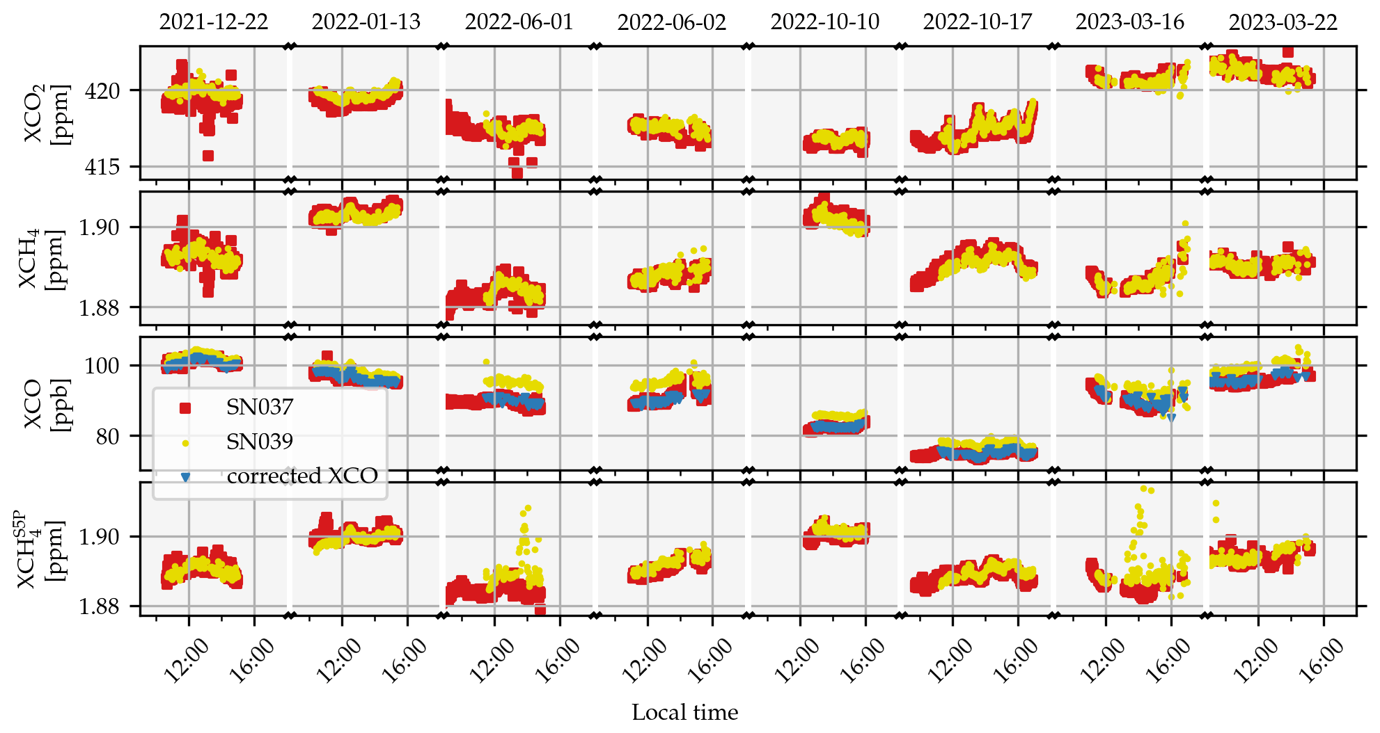
Figure 2 The result of the side-by-side measurements of the COCCON reference device using red squared markers and the TS using yellow dots. XCO₂, XCH₄ and XCO, and ${\mathrm{XCH}}_{\mathrm{4}}^{\mathrm{S}\mathrm{5}\mathrm{P}}$ are plotted in the top, middle, and bottom rows, respectively. For each of the gases, empirical bias compensation factors are calculated and summed up in Table 1. For XCO₂ and XCH₄, the correction show minor variability over time. For XCO, however, there is a significant variability. This variability is corrected using an ad hoc empirical function dependent on solar zenith angle. The corrected data are plotted using the blue triangle markers. From the corrected XCO data, only every 12th marker is plotted to provide a clearer figure. For more details, refer to Sect. 3.1.

A visual inspection reveals a good agreement and stable results for XAIR, XCO₂ and XCH₄ during all four measurement periods. For XCO, however, there is a larger difference in the second period (collected in Karlsruhe between the Japan and the Canada campaign), which is reduced again in the third period (collected in Karlsruhe between the Canada and the Australia campaign). A closer investigation of this behavior is given in Sect. 3.1, where an empirical correction for the variable XCO bias is derived. This correction is applied to the data of the TS spectrometer and plotted using the blue triangles in the figure. The increased noise levels (22 December 2021, 2 June 2022, 16 March 2023, 22 March 2023) are likely due to cloudy weather on these days. This results in higher DC variations of the interferograms and reduced quality of the solar tracking. Due to a tight schedule, it was necessary to also use non-perfect weather conditions.

Table 1 Tabulated bias compensation factors for the comparison of the TS spectrometer unit with the reference instrument. The bias compensation factors, $K_{\mathrm{SN}\mathrm{39}}^{\mathrm{SN}\mathrm{37}}$, are calculated using the data shown in Fig. 2. For XCO, the corrected values (red crosses) are used. $\mathrm{\Delta }{K}_{\mathrm{SN}\mathrm{39}}^{\mathrm{SN}\mathrm{37}}$ (%)​​​​​​​ denotes the deviation to the correction factor in the row above. $\mathrm{\Delta }\stackrel{\mathrm{‾}}{\text{XGas}}$ denotes the difference of the temporal mean over each measurement period. $\mathrm{\Delta }\left(\mathrm{\Delta }\stackrel{\mathrm{‾}}{\text{XGas}}\right)$ denotes the change of the difference to the previous encounter. For an evaluation of the stability of the instruments, the values of $\mathrm{\Delta }{K}_{\mathrm{SN}\mathrm{39}}^{\mathrm{SN}\mathrm{37}}$ and $\mathrm{\Delta }\left(\mathrm{\Delta }\stackrel{\mathrm{‾}}{\text{XGas}}\right)$ are the important values. The values (in %) for $\mathrm{\Delta }\left(\mathrm{\Delta }\stackrel{\mathrm{‾}}{\text{XGas}}\right)$ are given for a direct comparison with the estimated TCCON site-to-site consistency (column “MAD” of Table 5 in Laughner et al., 2024). To convert from the mixing ratio to percentage, we used 400 ppm for XCO₂, 1800 ppm for XCH₄ and 100 ppb for XCO. The smaller the $\mathrm{\Delta }\left(\mathrm{\Delta }\stackrel{\mathrm{‾}}{\text{XGas}}\right)$, the more stable the instruments are against each other. For all periods, the drift between two characterization measurements is less than the accuracy estimated for TCCON.

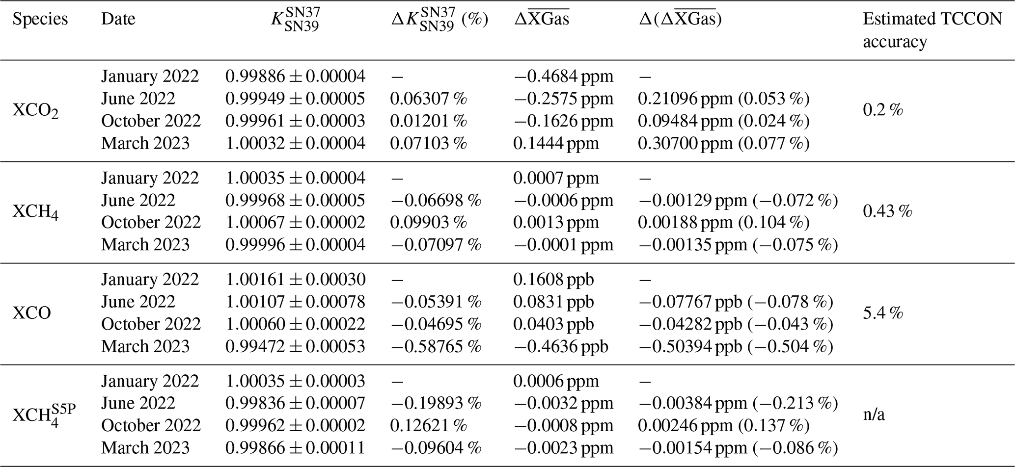
n/a: not applicable.

The bias compensation factors, i.e. $K_{\mathrm{SN}\mathrm{39}}^{\mathrm{SN}\mathrm{37}}$, are calculated and summarized in Table 1. For XCO, the corrected data are used to calculate the bias compensation factors. The errors are calculated using the procedure described in Sect. A1. Furthermore, the table shows the relative deviation of the correction factor to the row above (i.e., to the previous deployment in KA), i.e., $\mathrm{\Delta }{K}_{\mathrm{SN}\mathrm{39}}^{\mathrm{SN}\mathrm{37}}$, in percentage. In addition, for each measurement period the temporal mean of all XGas values is calculated for both the reference and the TS instrument, and the difference, i.e., $\mathrm{\Delta }\stackrel{\mathrm{‾}}{\text{XGas}}$, is calculated. The change in this quantity relative to the previous factor is given as $\mathrm{\Delta }\left(\mathrm{\Delta }\stackrel{\mathrm{‾}}{\text{XGas}}\right)$. The relative change of the correction factors in percentage, i.e., $\mathrm{\Delta }{K}_{\mathrm{SN}\mathrm{39}}^{\mathrm{SN}\mathrm{37}}$, and $\mathrm{\Delta }\left(\mathrm{\Delta }\stackrel{\mathrm{‾}}{\text{XGas}}\right)$ are used to check the stability of the two instruments.

The absolute change in the temporal mean values for all gases is less than the estimated site-to-site biases of the TCCON given in the introduction. From this, it can be seen that the stability of the TS EM27/SUN spectrometer is good enough for comparing TCCON stations.

It is assumed that the reference in Karlsruhe does not drift in time. This assumption is justified by a long-term analysis of the EM27/SUN reference spectrometer (SN37) with the TCCON-Karlsruhe data as shown in Alberti et al. (2022a), Fig. 20. Therefore, a deviation before and after a campaign is due to a change of the TS.

Hence, the presented difference gives an uncertainty to the final comparisons (compare with Appendix B and Fig. 16).

ILS analysis. A further monitoring tool is the measurement of the instrumental line shape (ILS) of the TS. The ILS is described by two values: the modulation efficiency (ME) and the phase error (PE). The ME and PE are described in Hase et al. (1999).

In short, assuming a monochromatic wave, the ME describes the decrease of the envelope of the sinusoidal interferogram towards higher optical path differences (OPDs). The phase error describes the shift of the zero crossings of the sinusoidal interferogram. Both values describe the deviation of a real-world instrument to a theoretical instrument. For a theoretically perfect instrument, one expects ME = 1 and PE = 0.

The ILS is measured before and after each visit. The results are plotted in Fig. 3.

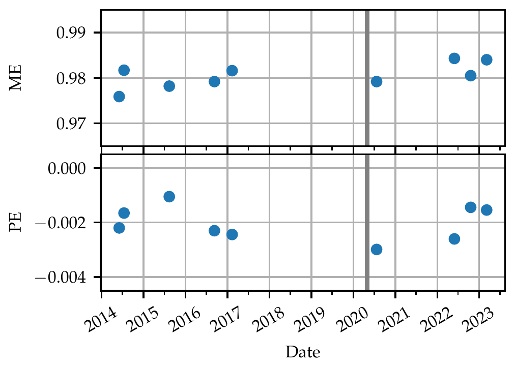
Figure 3 The ILS parameters of spectrometer SN39 used as the TS measured at different dates. It is described by the modulation efficiency (ME) and phase error (PE). The grey line indicates the date after which the measurements are relevant for this paper. The data before are plotted to show the values in the context of the history of the instrument.

The measurements collected before 2020 are not of relevance for the data evaluation of the TS, as always the newest available ILS value is used for the retrievals with PROFFAST2. However, they are listed in the figure to provide a comparison with the historical data of its ILS.

As a measure of the stability, the mean and the standard deviation of the ME and PE are calculated over all measurements in Fig. 3. This gives 0.98051±0.00272 for the ME and $-\mathrm{0.00202}\pm \mathrm{0.00063}$ for the PE. As a comparison, the mean and the standard deviation for the ME and PE values of the reference instrument SN037 as published in Alberti et al. (2022a) are ME = 0.98361 ± 0.00267 and PE = 0.00145 ± 0.00122. These values are on the same order of magnitude, showing that the ME and PE of the TS instrument are within the normal range of an EM27/SUN spectrometer.

3.1 Variable bias in XCO

To find the reason for the variable differences of the XCO product, several potential error sources have been investigated.

The first idea is that channeling might be responsible for the observed variations. Channeling describes the phenomenon of a thin element in the optical path which acts as a cavity and resonantly amplifies a certain frequency or integer multiples of it (Blumenstock et al., 2021). This has already been demonstrated by Frey (2018). This problem was ameliorated for all new EM27/SUN spectrometers by adding an antireflection coating on the long-pass filter. However, the SN039 instrument used as TS is the prototype version of the dual-channel setup (see Hase et al., 2016). In the laboratory, measurements to check for channeling as described by Frey (2018) are collected. They seem to be free of channeling, which does not support the thesis of channeling being the source of the deviation.

Next, a misalignment of the optics of the second channel could contribute to the variable XCO bias. To investigate this, a second XCH₄ product, called ${\mathrm{XCH}}_{\mathrm{4}}^{\mathrm{S}\mathrm{5}\mathrm{P}}$, which is retrieved from an alternative window within the range of the second channel is plotted in Fig. 2. This product does not show the same behavior as the XCO retrieval does. This can be seen also in Fig. 4 which shows the SZA dependency of XCH₄ and ${\mathrm{XCH}}_{\mathrm{4}}^{\mathrm{S}\mathrm{5}\mathrm{P}}$. In addition, the alignment of the second channel was checked by opening the instrument. Also by this method, no misalignment could be detected. The excellent agreement of XCH₄ and ${\mathrm{XCH}}_{\mathrm{4}}^{\mathrm{S}\mathrm{5}\mathrm{P}}$ also rules out an ILS problem or a zero baseline problem in the second channel.

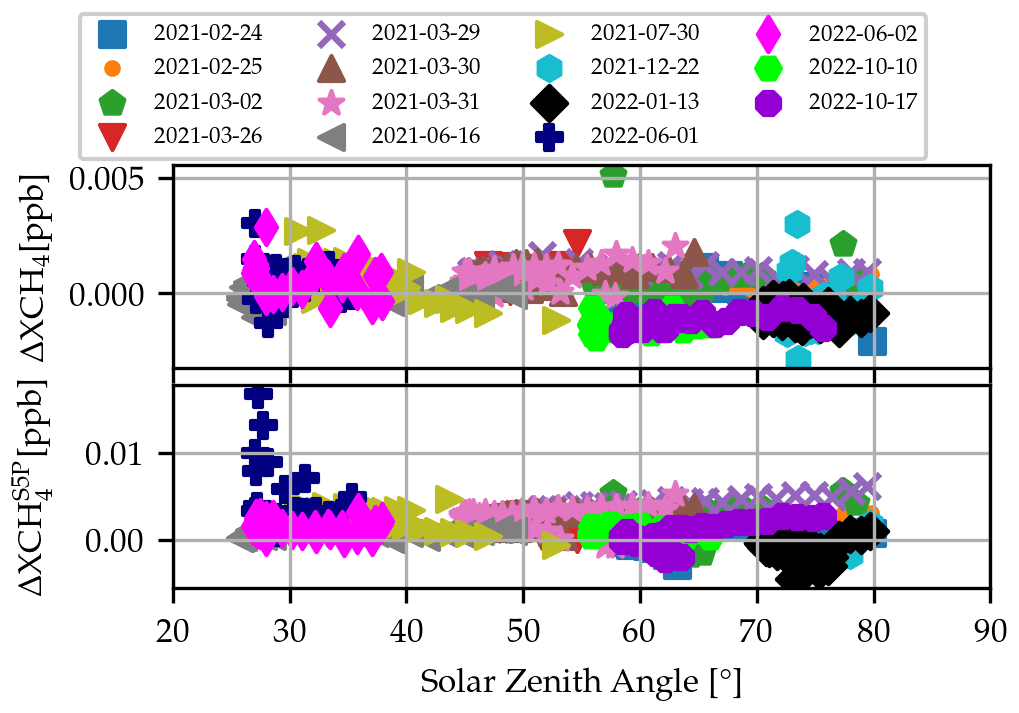
Figure 4 Investigating the dependency of ΔXCH₄ and $\mathrm{\Delta }{\mathrm{XCH}}_{\mathrm{4}}^{\mathrm{S}\mathrm{5}\mathrm{P}}$ of the EM27/SUN reference and the TS device as a function of the solar zenith angle (SZA). The data do not show a clear SZA dependence. This supports the thesis that there is no misalignment of the second channel causing the seasonal variability in XCO, because otherwise this would lead to the same dependency as given in Fig. 5 for XCO.

Fortunately, a larger dataset of side-by-side measurements exists covering 15 measurement days starting from 24 February 2021 until 17 October 2022. This dataset supports the hypothesis of an XCO bias which depends on the SZA. This is visualized in Fig. 5, where the ΔXCO between the reference instrument and the TS instrument is plotted as a function of the solar zenith angle.

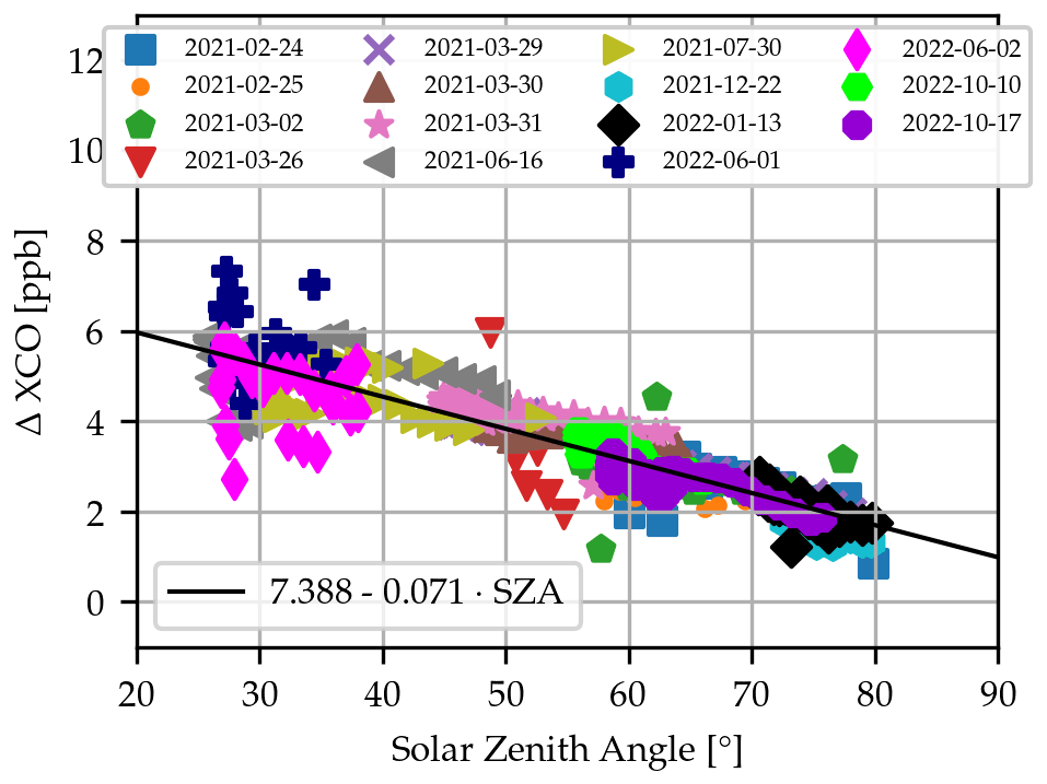
Figure 5 The ΔXCO of the EM27/SUN reference spectrometer and the TS device as a function the solar zenith angle (SZA). There is a clearly visible dependence on the SZA. The reason for this is still under investigation. However, this dependence is used to derive an empirical linear correction of the XCO values. The correction is applied to all measured data in this paper. In Fig. 2 the corrected XCO values are plotted using blue triangle markers.

From these data, it is possible to derive an empirical correction by fitting a linear regression line to the data. The result is the empirical correction function

$$\begin{array}{}\text{(4)}& c_{\mathrm{XCO}}\left(\text{SZA}\right)=\mathrm{7.39076}-\mathrm{0.071271}\cdot \text{SZA}\left(\mathit{°}\right),\end{array}$$

which is applied to all XCO data measured by the TS in this paper, except the data plotted in Fig. 2 in yellow squares to demonstrate the effect of the correction.

3.2 Verification of the pressure sensor used in the travel standard

The TS is equipped with a Vaisala PTB330 pressure sensor acquired in April 2021. Part of the verification performed at KIT is to also compare the pressure measurements collected by the TS sensor with the pressure data used for the Karlsruhe TCCON retrieval. For the Karlsruhe TCCON station, the pressure data of a nearby weather station (Rheinstetten, 15 km south-south-west of the TCCON station) of the German weather service (Deutscher Wetterdienst, DWD) are used. Unfortunately, there was an unnoticed crash of the program used to collect the pressure data of the TS sensor before the Tsukuba and the Canada campaign such that there are no side-by-side data for those periods. The only measurements are available after the Canada and Australia campaign. (For the evaluation of the solar side-by-side measurements, the pressure data recorded by the “rooftop sensor” (introduced below) are used.) They are plotted in Fig. 6. The data show an excellent agreement with the height-corrected data of the DWD-Rheinstetten station. The bias compensation factor between the TS and the DWD data is $K_{\mathrm{TS}}^{\mathrm{DWD}}\left(\text{Can}\right)=\mathrm{0.999813}$ and $K_{\mathrm{TS}}^{\mathrm{DWD}}\left(\text{Aus}\right)=\mathrm{0.999924}$ before and after the Australia campaign. The change of the bias compensation factors is −0.1 ‰. For further calculations, the average of both is used, which is $K_{{\mathrm{TS}}_{\mathrm{p}}}^{{\mathrm{DWD}}_{\mathrm{p}}}=\mathrm{0.999869}$. For an average pressure of 1000 hPa, this gives an average deviation of 0.131 hPa. According to the data sheet of the sensor (Vaisala, 2023), the accuracy of the sensor is 0.1 hPa. Therefore, the deviation to the DWD sensor is only slightly above the sensor's accuracy, which is an excellent agreement considering that the DWD station is 15 km away and the data are height corrected.

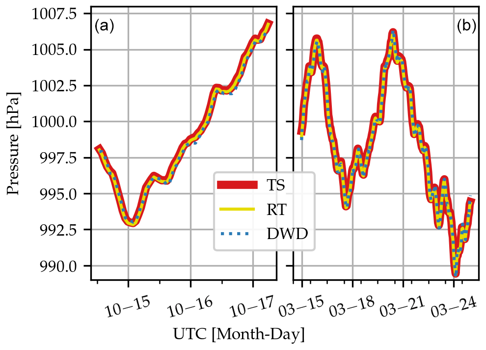
Figure 6 Measurements of the Vaisala PTB330 sensor in the TS compared with a weather station of the German weather service (DWD) in Rheinstetten and a second Vaisala PTB330 mounted permanently on the institute rooftop (RT). The measurements in panels (a) and (b) were collected in October 2022 (between Canada and Australia) and March 2023 (after Australia), respectively. For the comparison before and after Australia, a bias compensation factor of $K_{\mathrm{TS}}^{\mathrm{DWD}}\left(\text{Can}\right)=$ 0.999813 and $K_{\mathrm{TS}}^{\mathrm{DWD}}\left(\text{Aus}\right)=$ 0.999924 is found, respectively. The data of the Rheinstetten DWD station are corrected for an altitude difference of 17 m.

In Fig. 6 we plotted the measurements from another Vaisala PTB330 sensor measuring at the rooftop terrace on the seventh floor of the institute building. This sensor is called the rooftop (RT) sensor in the following. The agreement between the RT and the TS sensor is also excellent. The rooftop sensor collected data for longer than a year, so we can use its data as a proxy to investigate the stability of the PTB330 sensors. The comparison is shown as a scatter plot in Fig. 7. The data show an excellent agreement. A function $p_{\mathrm{RT}}\left(p_{\mathrm{DWD}}\right)=a\cdot p_{\mathrm{RT}}$ fitted to the data results in $a=\mathrm{0.999984}\pm \mathrm{3.061845}\times {\mathrm{10}}^{-\mathrm{6}}$. The deviation averaged over the whole period is 0.0138 hPa.

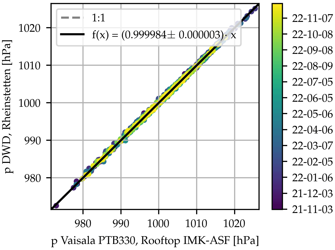
Figure 7 Results of the comparison of a Vaisala PTB330 mounted on the terrace of the institute building at the seventh floor and the DWD weather station in Rheinstetten at 16 km distant from the institute. The scatter plot shows an almost perfect agreement. The data do not show a drift in time. A linear function $p_{\mathrm{RT}}\left(p_{\mathrm{DWD}}\right)=a\cdot p_{\mathrm{RT}}$ fitted to the data gives $a=\mathrm{0.999984}\pm \mathrm{3.061845}\times {\mathrm{10}}^{-\mathrm{6}}$. The deviation averaged over the whole period is 0.0138 hPa, which is smaller than the accuracy of the PTB330 sensor which is 0.1 hPa (Vaisala, 2023). This shows the stability of the Vaisala PTB330 sensors.

This shows the high stability of the PTB330 sensors; hence, it is justified to use it as a reference with the TS.

4 Description of the TCCON and travel standard datasets collected in Tsukuba, Japan

In this section, we analyze the data recorded in Tsukuba, Japan. A quantitative comparison of the site-to-site bias is done in Sect. 7.2 together with the results of the other sites visited. The Tsukuba TCCON station is located at 31 m above sea level (m a.s.l.); the TS collected its measurements at an altitude of 39 m a.s.l. The TS was operated in Tsukuba from 24 March until 25 April 2022. In this period, we collected 8 d of measurements. The low-resolution data measured with the Tsukuba TCCON instrument will be denoted as TK-LR (Tsukuba-low-resolution), the standard TCCON data as TK-HR (high-resolution) and the data of the travel standard as TS.

Pressure analysis. As mentioned before, the TS is equipped with a Vaisala PTB330 pressure sensor. Unfortunately, during the first campaign of the TS in Tsukuba, the sensor was integrated into the enclosure such that the sensor was measuring the pressure within the enclosure. While analyzing the data after the campaign, we realized that the venting cooling fan in the enclosure produced a significant dynamic pressure inside the enclosure. As a consequence, the recorded pressure data were not usable for the retrieval. For future campaigns a tube was used which is connected to the inlet of the pressure sensor and ends at the outside of the enclosure to sample the surface pressure outside the enclosure.

Fortunately, a side-by-side measurement with the pressure sensor of the Tsukuba TCCON site was recorded with the fan turned off. Using this subset of data, it was possible to calculate a factor to map the data recorded with the pressure sensor of the Tsukuba TCCON site to the pressure sensor of the TS. Therefore, we used the pressure data from the official TCCON evaluation to retrieve the TS and TK-LR data. However, two corrections were applied to these data. The first is a correction to match the pressure sensor of the TS and the second is an altitude correction to account for the different altitudes of the TS and the TCCON measurements.

The pressure side-by-side measurements are plotted in Fig. D1. They were recorded from 23 April until 24 April 2022 each at midnight local time. Both datasets are resampled to 1 min bins. The Tsukuba pressure record is slightly lower than the TS record by −0.105 hPa, causing a bias compensation factor of $K_{{\mathrm{TK}}_{\mathrm{p}}}^{{\mathrm{TS}}_{\mathrm{p}}}=\mathrm{1.00010}$. The pressure offset is small enough that we do not expect it do influence the XGas retrieval.

XAIR analysis. In Fig. 8 the retrieved data of XAIR, XCO₂, XCH₄ and XCO are plotted. The TS data are plotted with blue dots, the TK-LR data are plotted with sandy stars and the TK-HR data are with red pentagons.

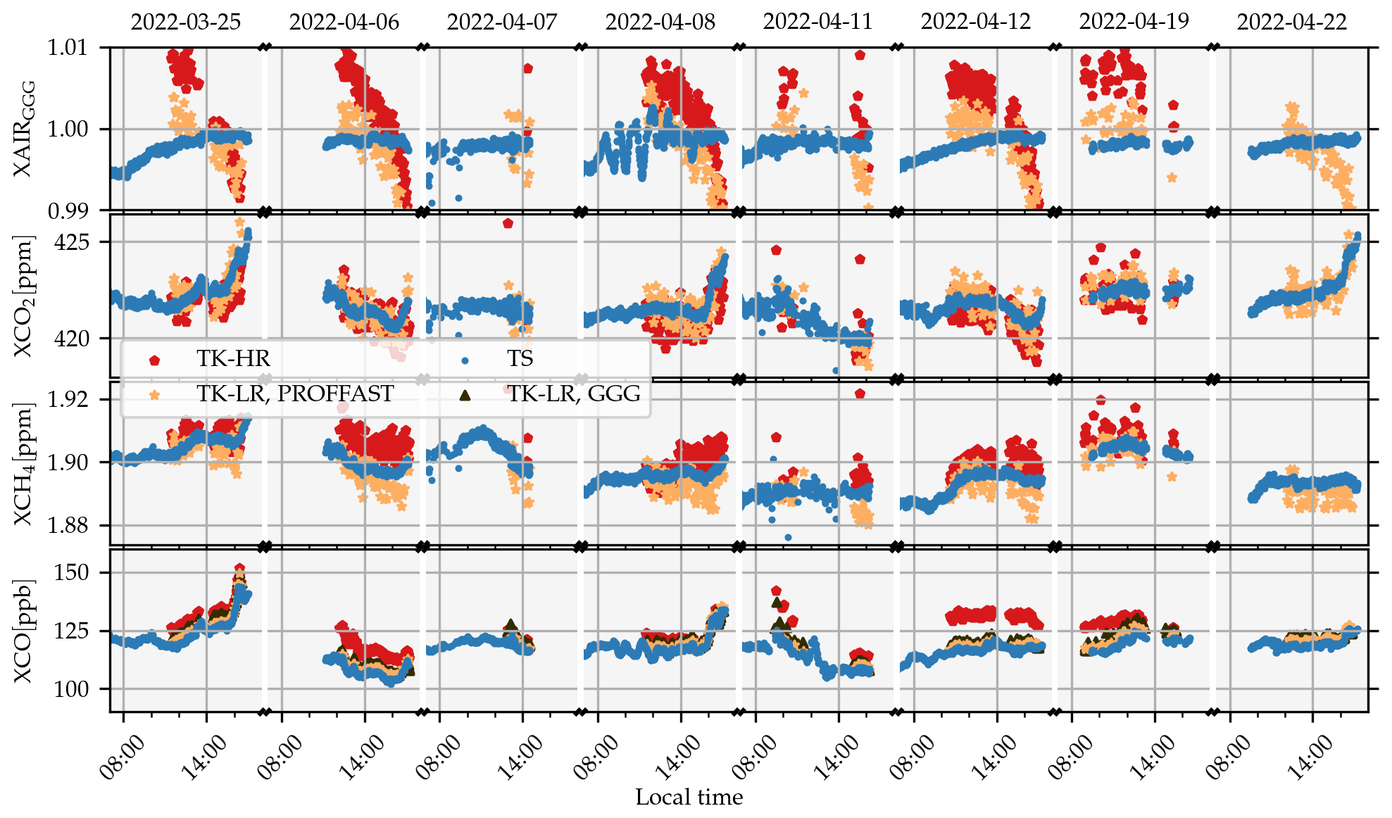
Figure 8 The XAIR, XCO₂, XCH₄ and XCO data of the side-by-side measurements in Tsukuba, Japan. The results of the retrieval of the TS are plotted with blue dots, the retrieved TK-LR data are plotted with sandy stars (both processed with PROFFAST2) and the retrieved TK-HR XGas values (processed with GGG2020) are plotted with red pentagons. One can see a good overall agreement for XCO₂ and XCH₄. For XCO, the agreement between the TK-HR and the TS data varies from day to day. This is caused by a combination of unrealistic a priori profiles and different spectral resolutions. Note that for XCO the TK-LR data are also processed with GGG2020 and plotted using black triangles. Furthermore, the TCCON results are noisier than the TS results. The origin of this is a signal drop towards higher wavenumbers in the spectrum. The fast oscillation of XAIR in the morning of 8 April 2022 is due to presumably non-hydrostatic pressure oscillations measured independently by the weather station of the Japan Meteorological Agency in Tsukuba, too. The subscript “GGG” at XAIR indicates that the XAIR values of PROFFAST are inverted to be comparable with the GGG XAIR values.

The TK-LR and TK-HR XAIR data show a clear air mass dependency over the course of the day. This is an indicator of an error in the recorded timestamp of the interferograms, which leads to a wrong calculation of the solar position. To correct this erroneous timestamp, empirically a correction of −44 s is found for the TK-LR data. The resulting data are plotted in Fig. C1 in the Supplement. It can be clearly seen that the air mass dependency of XAIR is almost completely eliminated by this. Furthermore, this also influences the XGas retrievals but to a much lesser extent. This is because to a first-order approximation the timing error cancels out when calculating XGas (compare with Eq. 1). The reason for this time offset is still under investigation and therefore no time-corrected TK-HR data are available yet. Note that the TK-HR data shown here are not the official TCCON product as the time error will be corrected before submitting the data to the TCCON database. TCCON is routinely doing a QA/QC check before publishing data, which is expected to discover such an error. However, this error was discovered first by the TS campaign data analysis.

Further analysis is conducted for both the corrected and uncorrected TK-LR data as well as for the uncorrected TK-HR data. The corrected data will be denoted as TK-LR-tcor and the uncorrected as TK-LR.

The XAIR values of the TS are normally distributed around unity. The only exception is 8 April 2022 where XAIR recorded by the TS oscillates during the morning hours. These oscillations seem to be induced by the pressure record, which shows the same oscillations as well. These oscillations are also detected by the weather station of the Japan Meteorological Agency in Tsukuba (Tateno) (Japan Meteorological Agency, 2023). These quasi-periodic pressure variations might be an effect of mountain wave activity generated by the surrounding summits. The wave activity in this area can be extreme as the loss of flight BOAC911 teaches (Dempsey, 2023).

Normally, one does not expect that a change in the surface pressure is influencing the XAIR retrieval. The reason why in this case the pressure variations can be seen in XAIR is the following: for the calculation of XAIR a hydrostatic atmosphere in equilibrium is assumed. However, in the presence of those waves hydrostatic equilibrium can no longer be assumed; hence, they directly disturb XAIR.

Fortunately, the oscillation of the pressure ends before the TCCON measurements are started; hence, it does not influence the side-by-side evaluation.

XAIR is designed such that it scatters around unity for an instrument that is aligned and set up well. Its distribution around unity is measured by calculating the mean value and the standard deviation of XAIR. This is 0.99796±0.00091 for the TS, 1.00224±0.00482 for the TK-HR and 0.99778±0.00357 for the TK-LR data. For the TK-LR-tcor data, it becomes 1.00028±0.00184. The values clearly show that the time correction improves the XAIR data significantly for the TK-LR data.

XGas analysis. For both the TK-HR and the TK-LR data, one can see high noise levels for XAIR, XCO₂ and XCH₄. This is due to a pronounced intensity drop for large wavenumbers in the Tsukuba TCCON spectra and is discussed in detail in Sect. 4.1.

For XCO₂ and XCH₄, a good agreement is found for the TS data and the TCCON data. Taking the average over all days and subtracting the TK data from the TS data gives an average bias over all days for XCO₂ of −0.0209 ppm and 0.2661 ppm for the low- and high-resolution data, respectively. For the TK-LR-tcor data, the bias is −0.0267 ppm. For XCH₄, we find a bias of 0.0028 ppm and −0.0046 ppm for the low- and high-resolution data and 0.0027 ppm for the TK-LR-tcor data. For XCO, the overall mean bias is −1.5997 ppb for the TK-LR data and −1.5768 ppb for the TK-LR-tcor data. In contrast, for the TK-HR data there are days with better agreement and others with worse agreement, resulting in an overall mean bias of −8.7191 ppb. To check if this is a problem with the PROFFAST retrieval software, the TK-LR data are also processed using GGG2020, plotted with black triangle markers. The day-to-day variability is similar to the TK-LR data processed with PROFFAST, even though the overall mean difference is 3.02 ppb larger. This indicates that it is not due to an issue with the PROFFAST code. Note that in Fig. 8 the GGG values are only plotted for XCO.

We therefore assume that the origin of the high day-to-day difference is due to a known issue with the CO a priori profiles shared by both analysis software packages, GGG and PROFFAST. The GEOS FP-IT model used for generating the priors incorporates an outdated emission inventory. This causes an overestimation of the CO a priori profiles in urban or energy-intensive areas. The resulting unrealistic CO a priori profile in combination with the different column sensitivities (due to the different spectral resolutions) causes the observed bias in the XCO data (Laughner et al., 2023a; Joshua L. Laughner, personal communication, 2023).

Investigation of high noise levels in TCCON XGas values

Despite the good mean agreement, the TK-LR XGas values have a noticeably higher noise than the TS values. The reason for this has been found in the retrieval of the O₂ column. All XGas values are calculated using Eq. (1). Hence, a high scattering in the O₂ column influences all other XGas values. This is depicted in Fig. 9, where the vertical column values of O₂ and CO₂ are plotted. One can see that for the TS data, the noise level of the CO₂ and O₂ are comparable. In contrast, for the TK-LR data, the O₂ column has a higher noise level than the CO₂ column.

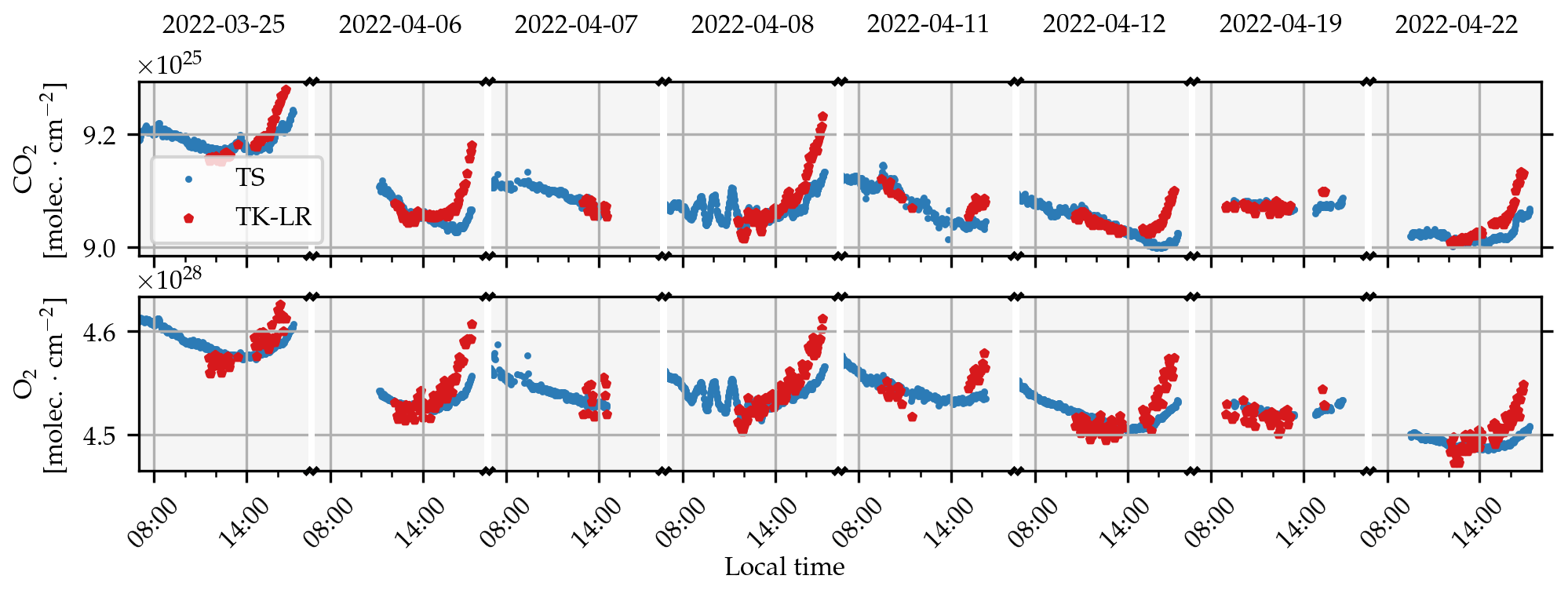
Figure 9 Retrieved total column values of CO₂ and O₂ for the TS data with blue dots and the TK-LR data with red pentagons. For the TK-LR data, the noise in the O₂ retrieval is much higher than it is for CO₂. This results in noisy XGas values which are shown in Fig. 8. The reason for this is a low signal level of the TCCON-LR spectra, as depicted in Fig. 10.

The reason for the high scattering in the O₂ retrieval was found in the shape of the spectra recorded by the TCCON spectrometer. It is shown in Fig. 10 in a light blue color. The maximum of the spectrum is normalized to unity. For illustration, a spectrum of the Karlsruhe TCCON station is plotted in yellow. (Since the Karlsruhe TCCON setup differs from the standard setup used in the TCCON, the Karlsruhe spectrum drops to zero at 5450 cm⁻¹. It is normalized such that its maximum matches with the spectrum height of the Tsukuba spectrum at the same wavenumber.)

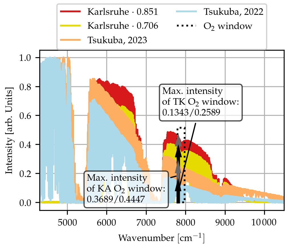
Figure 10 Comparison of the Tsukuba and the Karlsruhe spectra. The Tsukuba spectrometer has been realigned in early 2023. Therefore, a spectrum recorded during the TS visit in 2022 is plotted in light blue, and the realigned spectrum is plotted in sandy color. For comparison, the Karlsruhe spectrum is plotted in dark and light blue. The Tsukuba spectra are normalized to unity; the Karlsruhe spectra are normalized to match the intensity of the Tsukuba spectrum at 5680 cm⁻¹. The Karlsruhe spectrum in yellow is normalized to the 2023 Tsukuba spectrum, and the spectrum in red is normalized to match with the 2022 Tsukuba spectrum. The reason why the Karlsruhe spectrum drops to zero at 5450 cm⁻¹ is the non-standard TCCON setup in Karlsruhe. The Tsukuba spectra decrease strongly towards higher wavenumbers. However, after the realignment in 2023 the decrease is less intense. For the O₂ retrieval, the low signal level at the spectral position of the 1.26 µm O₂ band results in a bad signal-to-noise ratio and hence noisier XGas data. As a quantifying metric for assessing the spectrum, the maximum in the O₂ window is determined.

To characterize the observation in Tsukuba, two values were calculated. The first is the maximum value, ${max}_{{\mathrm{O}}_{\mathrm{2}}}$, within the O₂ window. The second value is the signal-to-noise ratio (SNR${}_{{\mathrm{O}}_{\mathrm{2}}}$) in the O₂ window. This was calculated by taking standard deviation, σ, of the parts of the spectra without signal (i.e., at the upper and lower end of the spectra or of points of zero transmittance). The signal-to-noise ratio is then calculated via ${\mathrm{SNR}}_{{\mathrm{O}}_{\mathrm{2}}}=\frac{{max}_{{\mathrm{O}}_{\mathrm{2}}}}{\mathit{\sigma }}$. The spectra are normalized to unity before doing this calculation.

As a consequence of this finding, the spectra of the TCCON visited with the TS plus several additional TCCON stations were checked. The results are summed up in Table 2.

Table 2 Analysis of various spectra recorded at different TCCON sites. The spectra were all recorded at around noon on a bright day. To make ${max}_{{\mathrm{O}}_{\mathrm{2}}}$ comparable, they are all normalized to unity. The value of ${max}_{{\mathrm{O}}_{\mathrm{2}}}$ is the maximum value in the O₂ window, ranging from (7800–7980) cm⁻¹. The noise is described by the standard deviation of the parts without signal. The signal-to-noise ratio is calculated by dividing the max value in the O₂ window by the calculated noise. One can see that there are large differences across the network.

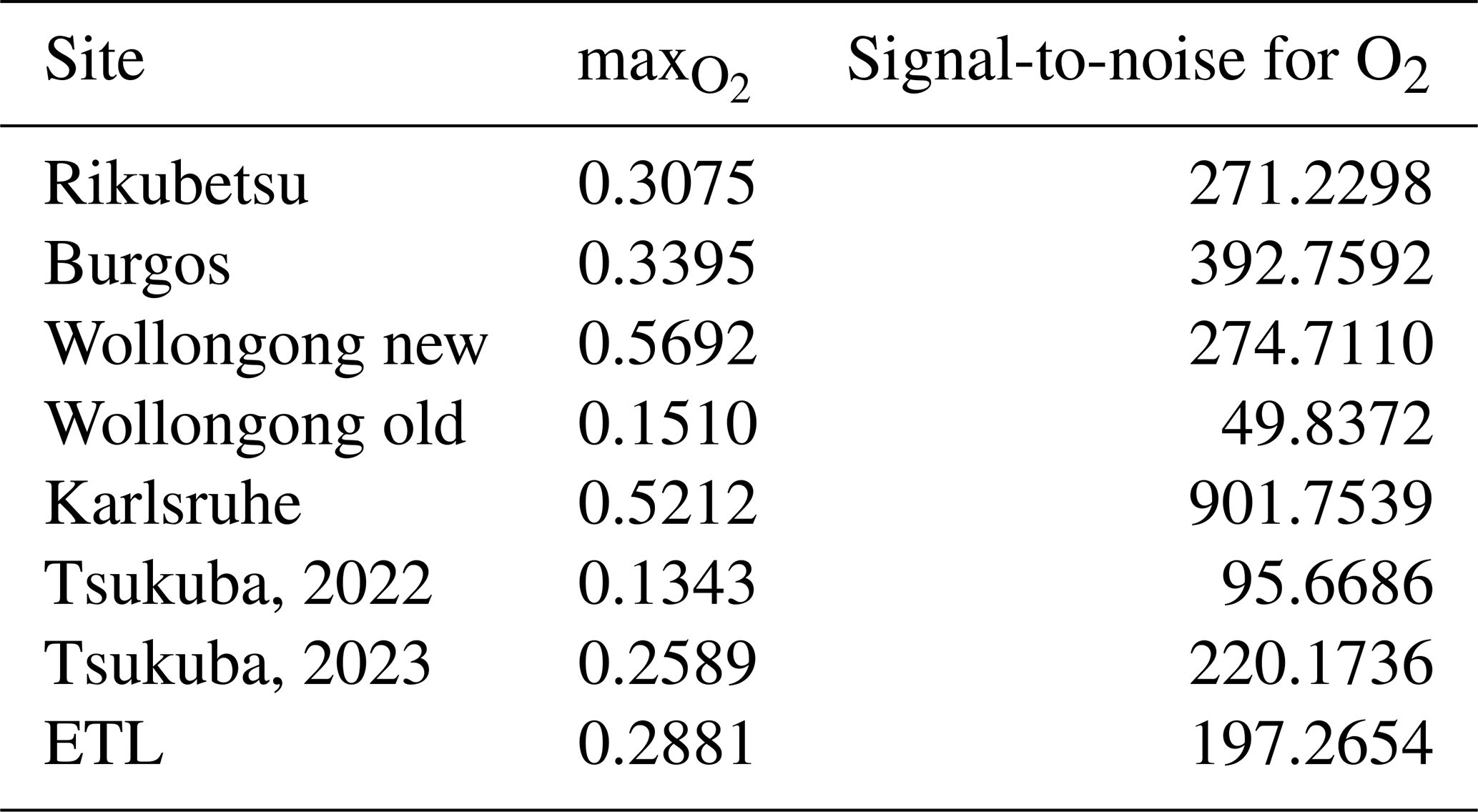
The results vary significantly across the sites. From this table, we expect high scatter also for the Wollongong station, which is confirmed by the later analysis (see Sect. 6). It is interesting to see that for sites that have set up a new instrument recently, the values are much better for the new instruments.

From the instrumental view point, this signal drop is likely created by the characteristics of the beam splitter and of the detector element. Also, mirror degradation and deterioration of other optical elements might have an influence on this. Furthermore, it is influenced by the alignment of the spectrometer: in early 2023 the Tsukuba spectrometer was realigned. This causes the intensity drop to be less pronounced. The realigned spectrum is plotted in Fig. 10 in sandy color, and in red is the Karlsruhe spectrum for comparison. In Table 2, the values for Tsukuba in 2022 and 2023 before and after the realignment are given.

5 Data analysis of ETL, Canada

One day before the TS arrived at the East Trout Lake (ETL) TCCON site in Canada, the reference laser of the TCCON spectrometer broke down. Consequently, it was not possible to perform the planned side-by-side measurements. Hence, there is unfortunately no direct comparison of station XGas measurements with the TS.

Pressure analysis. It was possible to record side-by-side pressure data in the range from 16 August 2022 at 08:00 until 17 August 2022 at 20:00 local time. The data are plotted in Fig. D2. The ETL data are recorded every second. The raw data have a high noise level; however, for the retrieval an average is calculated. For the comparison, both the TS and the ETL data are resampled in 1 min bins giving a good overall agreement. On average, the ETL pressure records are 0.00386 hPa higher than the TS pressure records. This results in a bias compensation factor of $K_{{\mathrm{TS}}_{\mathrm{p}}}^{{\mathrm{ETL}}_{\mathrm{p}}}=\mathrm{0.9999959}$.

XAIR analysis. The ETL TCCON spectrometer recorded 7 d of alternating high- and low-resolution measurements before the TS arrived. Furthermore, the TS recorded 3 d of data when arriving there. The data are plotted in Fig. 11. Still the data can be used to check for the noise level and for any anomalies in XAIR.

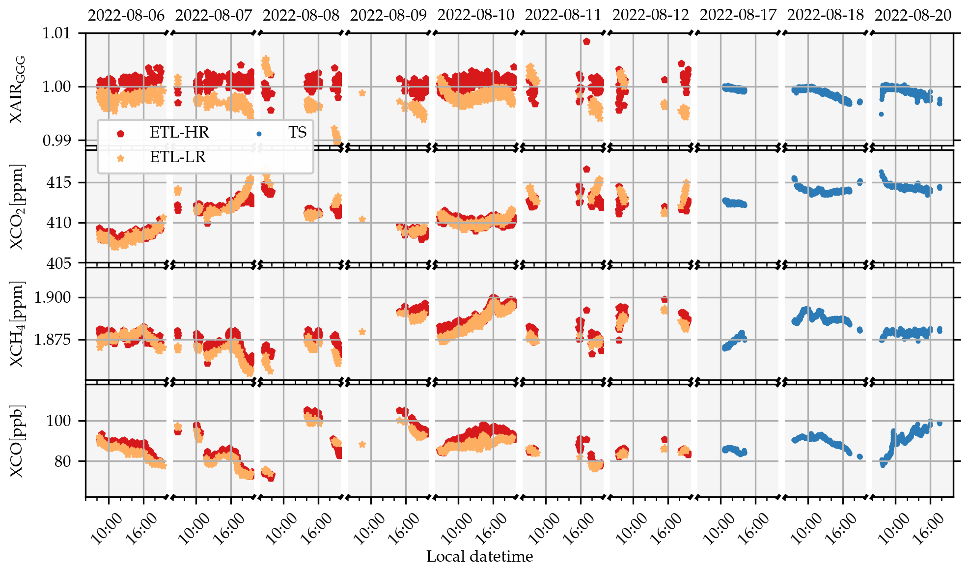
Figure 11 The retrieved XAIR and XGas values for the high- and low-resolution data in East Trout Lake (ETL), Canada. The data were recorded before the TS arrived. The reference laser of the ETL-TCCON spectrometer broke down when the TS was en route. Hence, no side-by-side measurements were possible. Nevertheless, the data are used for an XAIR and noise analysis. The subscript “GGG” at XAIR indicates that the XAIR values of PROFFAST are inverted to be comparable with the GGG XAIR values.

The visual analysis does not reveal any anomalies. As for the Tsukuba data, the mean and the standard deviation of XAIR are calculated. This gives 1.00043±0.00131 for the ETL-HR data, 0.99976±0.00163 for the ETL-LR data, and 1.00095±0.00082 for the TS data. The data are all close to unity with little noise. Hence, no instrumental problems are expected from this.

Furthermore, the data are used to check for the noise level. For this, the XAIR and the XGas values of the ETL-LR and ETL-HR data are analyzed. From a visual inspection, it is already apparent that the noise level is lower than it is for the Tsukuba data. A quantitative analysis is provided in Sect. 7.2.

6 Description of the TCCON and the TS datasets collected in Wollongong, Australia

The TS visited Wollongong (WG) from 6 December 2022 until 26 January 2023. In this period, 15 d of side-by-side measurements could be collected.

In Wollongong, there are currently two TCCON stations: an old one and a new one. The new one is not yet measuring continuously; hence, there are fewer data. The analysis in this work is therefore limited to the old instrument. The old instrument is located at −34°24^′21.6000^′′, 150°52^′44.4000^′′ at an altitude of 35 m a.s.l. The new instrument is located at −34°24^′21.6000^′′, 150°52^′48.0000^′′ at an altitude of 49 m a.s.l. The TS was placed on the rooftop next to the tracker of the new instrument but at an altitude of 48 m a.s.l.

Pressure analysis. The pressure sensors of the old and new TCCON site are at an altitude of 30 and 44 m a.s.l., and the TS sensor is at 48 m a.s.l. Hence, to compare the data, the records of the TS sensor are corrected for a height difference of −4 and −18 m, using the barometric height formula with a temperature of T=22 °C and the earth acceleration of g=9.81 m s⁻². The new TCCON and the corrected TS data are in good agreement with a small high bias of the TCCON data of 0.02517 hPa. The old TCCON and the corrected TS data agree with a small low bias of the TCCON data of 0.02517 hPa. This gives a bias compensation factor of $K_{{\mathrm{WG}}_{\mathrm{p}}}^{\mathrm{TS}}=\mathrm{1.0000373}$.

In Fig. D3 the pressure data collected during 2 d within this period are plotted. The days are chosen randomly. However, the analysis takes into account the whole dataset recorded during the visit.

Note that at the time this manuscript was written the altitudes of the TCCON pressure sensors and trackers remain with an uncertainty of around 1 m. The reason for this is that due to the visit of the TS an error in the so-far assumed altitudes of the pressure sensors and trackers was detected. The altitude of the tracker and the pressure sensors of the old TCCON site were assumed to be both at 30 m a.s.l. The altitude of the new tracker and pressure sensors were assumed to be at 34 and 30 m a.s.l. The new heights used here are determined using the pressure sensor of a smartphone.

The detection of this error is very important as the wrong height influences the retrieved XGas values. Furthermore, for the evaluation of the old TCCON data, the height difference of 5 m was not taken into account so far. This height difference leads to an approximate pressure difference of 0.58 hPa which is significant for the retrieval. As the GGG2020 dataset was not published at this time, the correction still could be included. For the GGG2014 dataset, however, this correction was not applied.

XAIR analysis. For the processing of the WG-LR and WG-HR data, the pressure data collected by the sensor at the old TCCON site with a height correction of 5 m is used. The data are plotted in Fig. 12. The WG-HR data are plotted using red pentagons, with the WG-LR data using sandy stars and the TS data using blue dots. A visual analysis shows a good agreement of the XAIR values for all three measurement products. The mean and the standard deviation of XAIR is 0.99957±0.00253 for the WG-HR data, 0.99881±0.00072 for the WG-LR data and 0.99885±0.00023 for the TS data. The high standard deviation of the TCCON data is due to the high noise level.

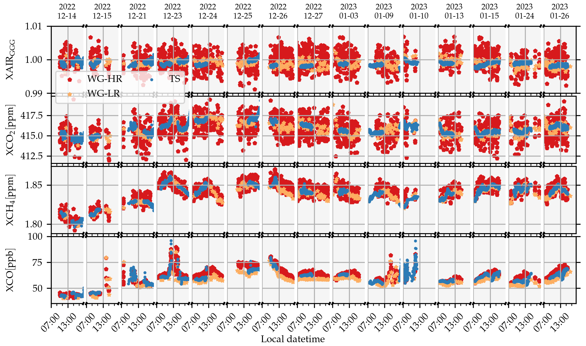
Figure 12 XAIR and XGas data of the Wollongong campaign. For all species, the overall agreement is good. It is interesting to see that the WG-HR data are much noisier than the WG-LR data. This is discussed in Sect. 7.1. Compared to the Tsukuba data, the difference of the XCO LR and HR data is smaller. This is probably due to better a priori profiles of the less urban area of Wollongong compared with Tsukuba. The subscript “GGG” at XAIR indicates that the XAIR values of PROFFAST are inverted to be comparable with the GGG XAIR values.

XGas analysis. In the following, the side-by-side measurements of the XGas values are discussed. Unfortunately, the WG-LR data were recorded with a low frequency, such that the timely distance between the measurements is on the order of 15 to 25 min. Hence, the bin size was chosen to be 30 min for the WG-LR data instead of 10 min as chosen for the Tsukuba measurement. The low data amount makes it difficult to derive reliable statistical values. Consequently, the results of the WG-LR data analysis might be less significant.

For XCO₂, XCH₄ and XCO, the WG-HR data show a high noise level, too. Interestingly, the noise level of the WG-LR data is less than it is for the HR data. The reason for this is a higher signal-to-noise ratio in the WG-LR spectra compared to the WG-HR spectra. This can be seen clearly in Fig. 13. This is discussed in more detail in Sect. 7.1.

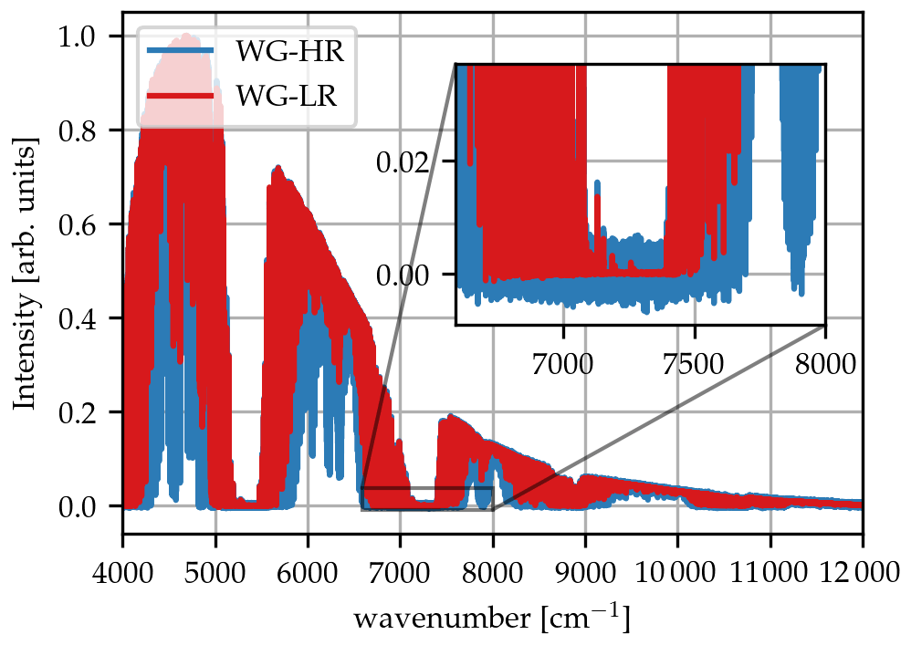
Figure 13 Comparison of the LR and HR data of the TCCON spectrometer in Wollongong. The HR data show a significantly worse signal-to-noise ratio than the LR data. This is clearly visible at the inset axes.

The overall agreement is good for all gases. For XCO₂, the averaged differences of the TS minus the WG data are 0.1316 and 0.1374 ppm for the WG-LR and WG-HR data, respectively. For XCH₄, the mean differences are 0.0005 and −0.0025 ppm for the LR and HR data. For XCO, the mean differences are 3.1902 and −1.2482 ppb for the LR and HR data.

Interestingly, for XCO the day-to-day differences of the HR and LR data are not as high as for the Tsukuba LR and HR data. This is probably because Wollongong is located in a more rural area than Tsukuba; hence, the CO priors are more realistic (compare with the end of Sect. 4).

7 Quantitative analysis of the data

7.1 Quantitative noise analysis

The reason for a higher noise level of the Tsukuba data is shown in Sect. 4.1. To make a quantitative analysis, the standard deviation of the time series of all TCCON products shown in the Figs. 8, 11 and 12 are calculated. This is done by calculating a rolling mean of data points which are temporally spaced less than 20 min and then calculating the standard deviation of the difference of the smoothed and the original data. This method is used to remove trends in the data.

The results are summed up in Table 3 and visualized in Fig. 14.

Table 3 Standard deviations, σ, of the XGas and XAIR values of the low- and high-resolution data of the visited TCCON sites. For all sites, the low-resolution data are less noisy than the high-resolution data, except for XCO of Wollongong. The data are visualized in Fig. 14.

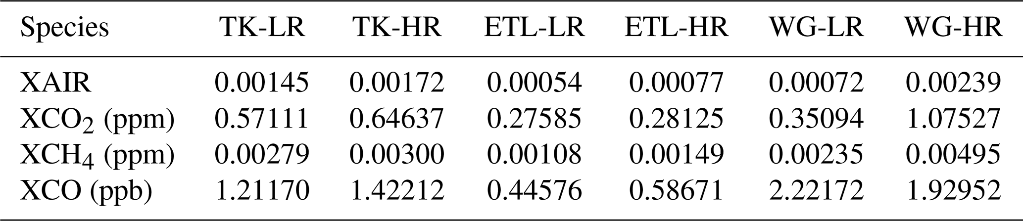
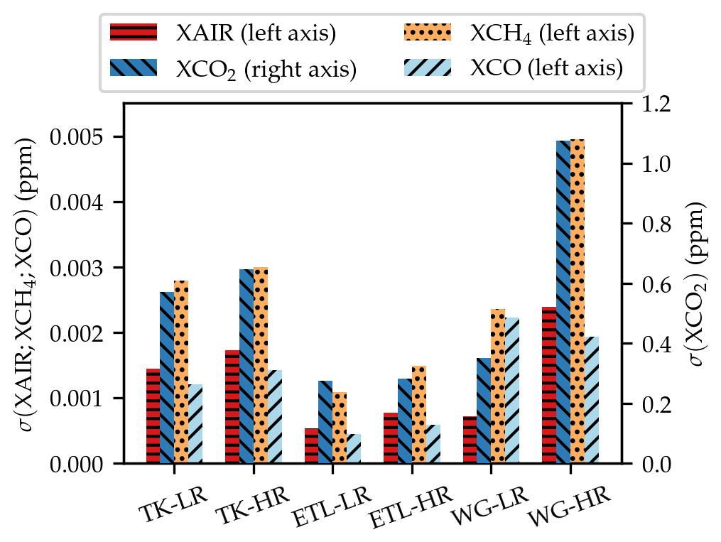
Figure 14 Visualization of the standard deviations as a measure of the noise in the XGas time series of the sites visited with the TS. The data of the plot are also given in Table 3. This clearly shows the different performances with respect to noise of the different TCCON spectrometers. Note that XCO₂ refers to the y axis on the right and all other gases refer to the y axis on the left. XCO is plotted in ppm to increase its visibility.

The different noise levels which can be estimated already from the time series plots of the data are also confirmed quantitatively. One can see that for all gases, except for XCO in Wollongong, the noise level for the LR data is lower than for the HR data. This is reasonable for the interplay of two reasons: on the one hand, the spectral noise in an FTIR measurement increases steeply with maximum optical path difference (Davis et al., 2001). On the other hand, a less resolved spectrum is not resolving the spectral absorption lines as clear as a more resolved spectrum. Hence, strong absorbers like CO₂ or CH₄ are well resolved even with a low-resolution spectrometer. Hence, they can profit from the higher spectra signal-to-noise ratio of a low-resolution spectrum. In contrast, weak absorbers like CO are not as well resolved in a low-resolution spectrum and hence are often better retrieved from high-resolution spectra.

7.2 Derivation of the XGas station-to-station bias

In this section, the TCCON sites are quantitatively compared relative to the Karlsruhe TCCON site. The choice to use Karlsruhe as a reference was made since the COCCON reference device is regularly tied to the Karlsruhe TCCON station. This does not imply that the Karlsruhe TCCON serves as an absolute reference to the whole TCCON network. But the use as reference for relative comparisons is an obvious choice.

Technically, the comparison is made by the usage of gas-specific bias compensation factors. They are determined as described in Appendix A. In the following it is assumed that the bias compensation factors fully describe the systematic bias between two spectrometers. Hence, in this ideal assumption we can write

$$\begin{array}{}\text{(5)}& \stackrel{\mathrm{‾}}{{\text{XGas}}_{\mathrm{XX}}}=\stackrel{\mathrm{‾}}{{\text{XGas}}_{\mathrm{YY}}}\cdot K_{\mathrm{YY}}^{\mathrm{XX}},\end{array}$$

where $\stackrel{\mathrm{‾}}{{\text{XGas}}_{\mathrm{XX}/\mathrm{YY}}}$ is the temporal mean of device XX or YY, respectively. This allows us to retrieve a virtual bias compensation factor to compare the TCCON site visited with the TS to the Karlsruhe TCCON site. This is done by the multiplication of the bias compensation factors retrieved before each campaign in Karlsruhe (see Sect. 3) with the factors retrieved during the campaigns (given in Table A1). This scheme is depicted in Fig. 15 and described in Appendix B1. The resulting correction factors are given in Table A2.

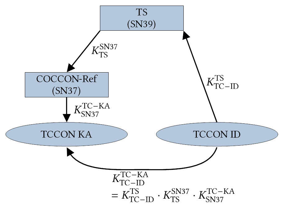
Figure 15 A graphical representation on how to use the bias compensation factors to compare the measurements of a visited TCCON site to the Karlsruhe TCCON site.

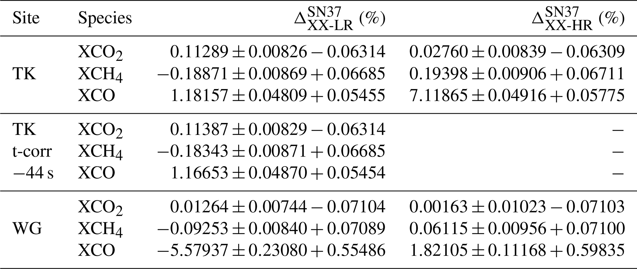
To derive a more intuitive comparison, the bias compensation factors comparing the visited TCCON sites to the reference in Karlsruhe are used to calculate deviations in percentage. The calculations for this are given in Appendix B1. The resulting values are given in Table 4.

To assess the quality of the comparison, it is crucial to do an error analysis for these virtual bias compensation factors. For this, two different contribution factors are considered: the first is the random error originating from the individual bias compensation factors as described in Appendix A. The random error is given with a “±” sign. The second is an uncertainty introduced by a potential drift of the TS instrument relative to the COCCON reference. Here, the upper limit of this uncertainty is estimated by using the $\mathrm{\Delta }{K}_{\mathrm{SN}\mathrm{39}}^{\mathrm{SN}\mathrm{37}}$ of the bias compensation factors measured before and after each campaign as given in Table 1. The details of the error calculation are given in Appendix B.

The error calculation was conducted for the bias compensation factors in Table A1 as well as for the deviations in percentage in Table 4.

Table 4 The table gives the deviations in percentage of the visited TCCON sites to the reference in Karlsruhe. The first error given is the random error emerging from the noise of the measurements. Second, a calibration uncertainty is given, which is calculated by considering a potential drift of the TS device relative to the COCCON reference device (derived from the $\mathrm{\Delta }\left(\mathrm{\Delta }\stackrel{\mathrm{‾}}{\text{XGas}}\right)$ in Table 1).

7.3 Discussion of the quantitative TS vs. TCCON comparison

In this section, we discuss the quantitative comparison of the visited TCCON sites to the reference in Karlsruhe. The direct comparison of the visited TCCON sites to the reference in Karlsruhe as a deviation in percentage is given in Table 4. In Fig. 16, the data results are visualized. For the creation of Fig. 16, we assume that the TCCON site-to-site error budget is distributed evenly around the Karlsruhe reference level. The error bars are dominated by the calibration error introduced by the comparison of the TS unit SN39 with the COCCON reference unit SN37.

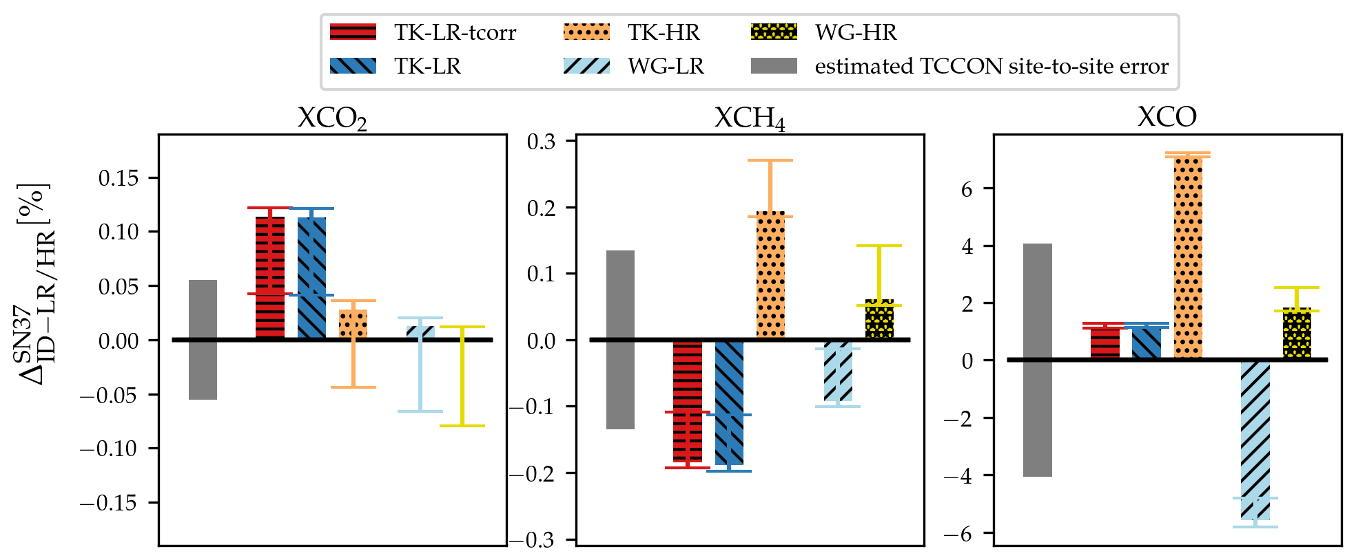
Figure 16 Results of the campaigns in Tsukuba, Japan, and Wollongong, Australia. The three panels show the results for each species. In grey, the TCCON error budget as estimated in Laughner et al. (2024) (Table 3, column “Mean abs. dev.”) is plotted. The data of this plot are also given in Table 4.

For the following discussion, it is important to keep in mind that the comparison of the HR data are affected by variable smoothing error contributions resulting from the different vertical sensitivities of low- and high-resolution measurements. This introduces an uncertainty when comparing XGas results.

For XCO₂, when assuming an evenly distributed TCCON site-to-site error budget around the TCCON-KA level, as shown in Fig. 16, the deviation of the Tsukuba-LR data are outside of the error budget; all others are within the budget. The correction of the timing error in the TK-LR data does not have a large effect.

For XCH₄, the low- and high-resolution data of both the Tsukuba and the Wollongong data deviate in the opposite directions. Future employments of the TS will tell whether this is a general feature of XCH₄. The WG data are within the TCCON site-to-site deviation budget, whereas this is not the case for the TK data, assuming again the TCCON deviation budget is evenly distributed. For TK, the time correction slightly decreases the deviation.

For XCO and a centered deviation budget, the deviations for TK-HR and WG-HR are larger than the budget; the rest is within the budget. The reasons for that are the following. First the already discussed deviation of the TK-HR and the TK-TS data is visible clearly, which is caused by the unrealistic CO a priori profile. In contrast, the TK-LR results are almost within the error budget.

For Wollongong, the WG-LR data are suffering from the low sample frequency and hence are not able to resolve the high temporal variability of XCO. This can be seen nicely for the data recorded on 23 December 2022. There, a large peak in the XCO data is visible. However, the low-sampled WG-LR data are not able to sample this peak appropriately. Hence, when comparing data with very different sampling rates this can cause large differences.

Pressure data

The pressure data collected at each site are summed up here and compared to the DWD Rheinstetten data by multiplying the bias compensation factors: $k_{{\mathrm{ID}}_{\mathrm{p}}}^{{\mathrm{DWD}}_{\mathrm{p}}}=k_{{\mathrm{TS}}_{\mathrm{p}}}^{{\mathrm{DWD}}_{\mathrm{p}}}\cdot k_{{\mathrm{ID}}_{\mathrm{p}}}^{{\mathrm{TS}}_{\mathrm{p}}}$. Assuming a pressure value of 1000 hPa the factors are used to calculate an absolute difference in hPa by ${\mathrm{\Delta }}_{\mathrm{ID}}^{\mathrm{DWD}}=\mathrm{1000}\cdot \left(\mathrm{1}-k_{{\mathrm{ID}}_{\mathrm{p}}}^{{\mathrm{DWD}}_{\mathrm{p}}}\right)$. The largest deviation is found at the ETL site with a deviation of 0.135 hPa which is still a very low deviation. Hence, all sensors show an excellent agreement.

The pressure analysis is very important as it revealed the issues with the assumed height of the TCCON site in Wollongong as well as the not applied height correction for the TCCON analysis. An altitude of 5 m leads to a pressure difference of approximately 0.58 hPa. A study of Tu (2019) using PROFFIT as an evaluation software with low-resolution spectra, a change of 1 hPa in the measured ground pressure causes an average increase of about 0.035% in XCO₂, 0.039% in XCH₄ and 0.052% in XCO, respectively. According to the measured level of pressure deviations, we do not expect them to have a large influence on the XGas values.

Table 5 Deviation of the pressure data recorded at the TCCON-site to the pressure sensor included to the TS and to a measurement station of the German weather service (DWD). The deviation in hPa is calculated by assuming a pressure of 1000 hPa.

8 Conclusions

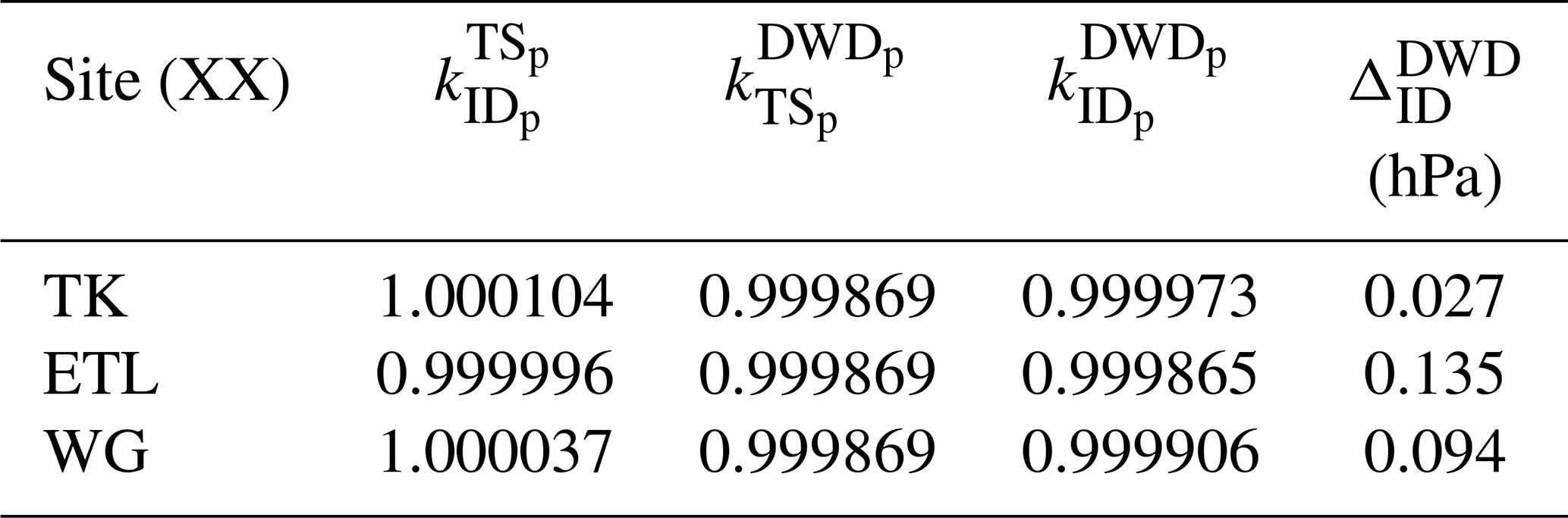
In this paper, we successfully demonstrated the usage of an EM27/SUN spectrometer as an international travel standard (TS) for the TCCON network. It was deployed to four TCCON sites on different continents: Tsukuba in Japan, East Trout Lake in Canada, Wollongong in Australia and Karlsruhe in Germany. Karlsruhe is the home base of the TS instrument and hosts the COCCON reference spectrometer. Therefore, the TCCON site Karlsruhe has been chosen as a reference for relative comparisons.

Before and after each campaign at a TCCON site, the TS performed side-by-side measurements with the COCCON reference spectrometer located in Karlsruhe and the colocated TCCON-Karlsruhe instrument. Using these data, bias compensation factors are calculated to tie the TS instrument to the Karlsruhe TCCON site.

At each site, the TS measured side-by-side with the TCCON instrument for several days. In the period the TS was visiting a TCCON site, the TCCON instrument measured two different data products in an alternating way: the standard high-resolution TCCON data (XX-HR) and low-resolution data (XX-LR) with a maximal optical path difference of 1.8 cm, matching the resolution of the EM27/SUN. For both data products, a bias compensation factor to the TS was calculated. By multiplying those factors with the bias compensation factors tying the TS to the COCCON reference, the visited TCCON sites are compared to the Karlsruhe TCCON site as a common reference.

At the Tsukuba site, a systematic error of the timestamp of the recorded interferograms was found to be −44 s during the campaign. For the TK-LR data, this error could be corrected, and the analysis is carried out for both the corrected and uncorrected TK-LR data. In Tsukuba as well as in Wollongong, high noise was found for XGas products, which was traced back to a low signal level in the spectral O₂ window. In East Trout Lake, Canada, an important part of the TCCON instrument broke in the night before the TS arrived. Consequently, it was not possible to do a quantitative comparison.

The agreement found in Tsukuba and Wollongong for XCO₂ is on the 0.1 % level. For XCH₄, the agreement is within 0.2 %, which is also a very satisfying result. For both the Tsukuba and the Wollongong data, the low-resolution XCH₄ data are biased low compared to the high-resolution data. This is an interesting issue to be investigated in future campaigns.

For XCO, the deviations are larger than the TCCON requirements (several %) and are less consistent. However, the comparison of the Tsukuba data seem to suffer from unrealistic a priori profiles. The WG-LR data suffer from a low sampling frequency which probably causes the large differences and hence cannot sample structures like the large peak on 23 December 2022 accurately. A summation of the results is given in Fig. 16.

The TS is equipped with a pressure sensor which allows us to compare the pressure records of the different TCCON sites to a pressure station at the German weather service (DWD), which is used for the Karlsruhe TCCON evaluation. The bias compared to the DWD station is 0.027 hPa for the Tsukuba pressure records, 0.136 hPa for the ETL pressure records and 0.094 hPa for the Wollongong pressure records. In Wollongong, the comparison of the pressure measurements revealed an error in the assumed heights of the sensor and the tracker, which will be corrected in the official GGG2020 data.

To make use of the valuable insights provided by the TS, it would be desirable to visit TCCON sites regularly. However, the TS activities take quite some effort as can be seen in this study. Continuing with the same speed would take around 10 years to visit all the TCCON sites (∼ 3 yr⁻¹). To speed this up, different approaches are possible: the most direct one, which is already planned, would be to use several closely monitored EM27/SUN devices to be used as TS in parallel sharing the same enclosure. This helps to increase the frequency of campaigns as one of the EM27/SUN spectrometers can be sent to a campaign while in parallel the other can perform side-by-side measurements in KA. Also, it would be possible to visit several sites between two calibration stops at KA. However, this would reduce the accuracy as the TS is less closely monitored. Another approach would be to visit one TCCON site per country and transfer its level to surrounding sites by using other EM27/SUN spectrometers, which, of course, must be monitored closely, too.

For future campaigns, several lessons can be learned from this study: pressure measurements shall not be measured inside a box with a venting fan (this issue was addressed after the Japan campaign). The TS requires a close monitoring of instrumental performance between deployments. The observation periods on site need to span sufficient time periods to reduce the random error budget. The XCO performance of the TS needs further evaluation.

Appendix A: Determination of bias compensation factors

To compare the XGas results of two different spectrometers, in this work empirical relative bias factors are established. We assume these are air mass independent. They are used to describe the difference of a species XGas of instrument XX to the instrument YY regarded as reference and is denoted as $K_{\mathrm{XX}}^{\mathrm{YY}}\left(\text{XGas}\right)$.

The procedure for all bias compensation factors calculated in the course of this paper is always identical.

First, the data are filtered as described in Sect. 2.2.2. To derive the factors, the filtered XGas values of both instruments XX and YY are binned in intervals of l min, denoted as ${\stackrel{\mathrm{‾}}{\text{XGas}}}_{\mathrm{XX}}^{t_i}$, where t_i is enumerating the bins. Considering all coincident bins of both instruments, the bias compensation factor is calculated by dividing the values of instrument YY by the ones of instrument XX and computing the average

$$\begin{array}{}\text{(A1)}& {\displaystyle }{K}_{\mathrm{XX}}^{\mathrm{YY}}={\displaystyle \frac{\mathrm{1}}{N}}\sum _{i=\mathrm{coincident}\mathrm{bins}}^N{\displaystyle \frac{{\stackrel{\mathrm{‾}}{\text{XGas}}}_{\mathrm{YY}}^{t_i}}{{\stackrel{\mathrm{‾}}{\text{XGas}}}_{\mathrm{XX}}^{t_i}}}\text{(A2)}& {\displaystyle }={\displaystyle \frac{\mathrm{1}}{N}}\sum _{i=\mathrm{coincident}\mathrm{bins}}^N{\left(q_{\mathrm{XX}}^{\mathrm{YY}}\right)}^i,\end{array}$$

Here, $(q_{\mathrm{XX}}^{\mathrm{YY}}{)}_i=\frac{{\stackrel{\mathrm{‾}}{\text{XGas}}}_{\mathrm{YY}}^{t_i}}{{\stackrel{\mathrm{‾}}{\text{XGas}}}_{\mathrm{XX}}^{t_i}}$.

A1 Error analysis of the bias compensation factors

The error of a measurement can be split into a systematic and a random error. Under constant conditions a systematic error falsifies repeated measurements by the same amount. In contrast, a random error is randomly influencing the results. The systematic errors of the TCCON stations and the TS give rise to the detected biases as described by the bias compensation factors. Here, we consider the random errors, which limits our ability to determine the correct bias compensation factors from a limited number of measurements. The random error is described by the standard error,

$$\begin{array}{}\text{(A3)}& s_i^{\mathrm{ID}}={\displaystyle \frac{{\mathit{\sigma }}_i^{\mathrm{ID}}}{{\sqrt{n_i}}^{\mathrm{ID}}}},\end{array}$$

of the data, with ${\mathit{\sigma }}_i^{\mathrm{ID}}$ being the estimated standard deviation of the data of an instrument ID, and n_i being the number of measurements in bin i. When binning the data in the intervals of I minutes, we compute the standard error for each instrument in each I min bin

The Gaussian error propagation of the relative error for the case of a quotient $x=\frac{x_{\mathrm{1}}}{x_{\mathrm{2}}}$ or a product $x=x_{\mathrm{1}}\cdot x_{\mathrm{2}}$ is (see Kaloyerou, 2018),

$$\begin{array}{}\text{(A4)}& {\displaystyle \frac{\mathit{ϵ}\left(x\right)}{x}}={\left[{\left({\displaystyle \frac{\mathit{ϵ}\left(x_{\mathrm{1}}\right)}{x_{\mathrm{1}}}}\right)}^{\mathrm{2}}+{\left({\displaystyle \frac{\mathit{ϵ}\left(x_{\mathrm{2}}\right)}{x_{\mathrm{2}}}}\right)}^{\mathrm{2}}\right]}^{\frac{\mathrm{1}}{\mathrm{2}}}.\end{array}$$

Here, ϵ(x) describes the error on a quantity x. We use this notation to indicate that the error is not equal to the standard deviation and also to avoid confusion with the difference of two values which is denoted as Δ.

Using Eq. (A4), the relative error for the quotient of the ith bin is calculated by

$$\begin{array}{}\text{(A5)}& {\displaystyle \frac{\mathit{ϵ}{\left(q_{\mathrm{XX}}^{\mathrm{YY}}\right)}_i}{{\left(q_{\mathrm{XX}}^{\mathrm{YY}}\right)}_i}}={\left[{\left({\displaystyle \frac{s_i^{\mathrm{XX}}}{{\stackrel{\mathrm{‾}}{\text{XGas}}}_{\mathrm{XX}}^{t_i}}}\right)}^{\mathrm{2}}+{\left({\displaystyle \frac{s_i^{\mathrm{YY}}}{{\stackrel{\mathrm{‾}}{\text{XGas}}}_{\mathrm{YY}}^{t_i}}}\right)}^{\mathrm{2}}\right]}^{\frac{\mathrm{1}}{\mathrm{2}}}.\end{array}$$

The error of the final bias compensation factor is calculated using the Gaussian error propagation of Eq. (A1).

$$\begin{array}{}\text{(A6)}& \mathit{ϵ}\left(K_{\mathrm{XX}}^{\mathrm{YY}}\right)={\left[{\displaystyle \frac{\mathrm{1}}{N^{\mathrm{2}}}}\sum _{i=\mathrm{1}}^N{\left(\mathit{ϵ}{\left(q_{\mathrm{XX}}^{\mathrm{YY}}\right)}_i\right)}^{\mathrm{2}}\right]}^{\frac{\mathrm{1}}{\mathrm{2}}}.\end{array}$$

Note that because Eq. (A1) is a sum, the absolute errors $\mathit{ϵ}{\left(q_{\mathrm{XX}}^{\mathrm{YY}}\right)}_i$ and not the relative errors $\frac{\mathit{ϵ}{\left(q_{\mathrm{XX}}^{\mathrm{YY}}\right)}_i}{{\left(q_{\mathrm{XX}}^{\mathrm{YY}}\right)}_i}$ are used. However, the errors given in the paper are the relative errors, which are $\frac{\mathit{ϵ}\left(K_{\mathrm{XX}}^{\mathrm{YY}}\right)}{K_{\mathrm{XX}}^{\mathrm{YY}}}$.

A2 Tabulated bias compensation factors

To compare a visited TCCON site with the reference in Karlsruhe, several of the bias compensation factors between different instruments must be multiplied. This is depicted in Fig. 15. In the main part of this paper, only the resulting bias of the TCCON sites relative to the reference in Karlsruhe ($K_{\mathrm{XX}\text{-}\mathrm{HR}/\mathrm{LR}}^{\mathrm{SN}\mathrm{37}}$) in percentage are given. The intermediate bias compensation factors between the visited TCCON sites and the TS are given in Table A1.

Table A1 The bias compensation factors for the TCCON-HR, and -LR data of the TK and WG sites to the TS (SN39). For the Tsukuba data, also the time-corrected LR data are given. The XX stands for the two letter TCCON-ID.

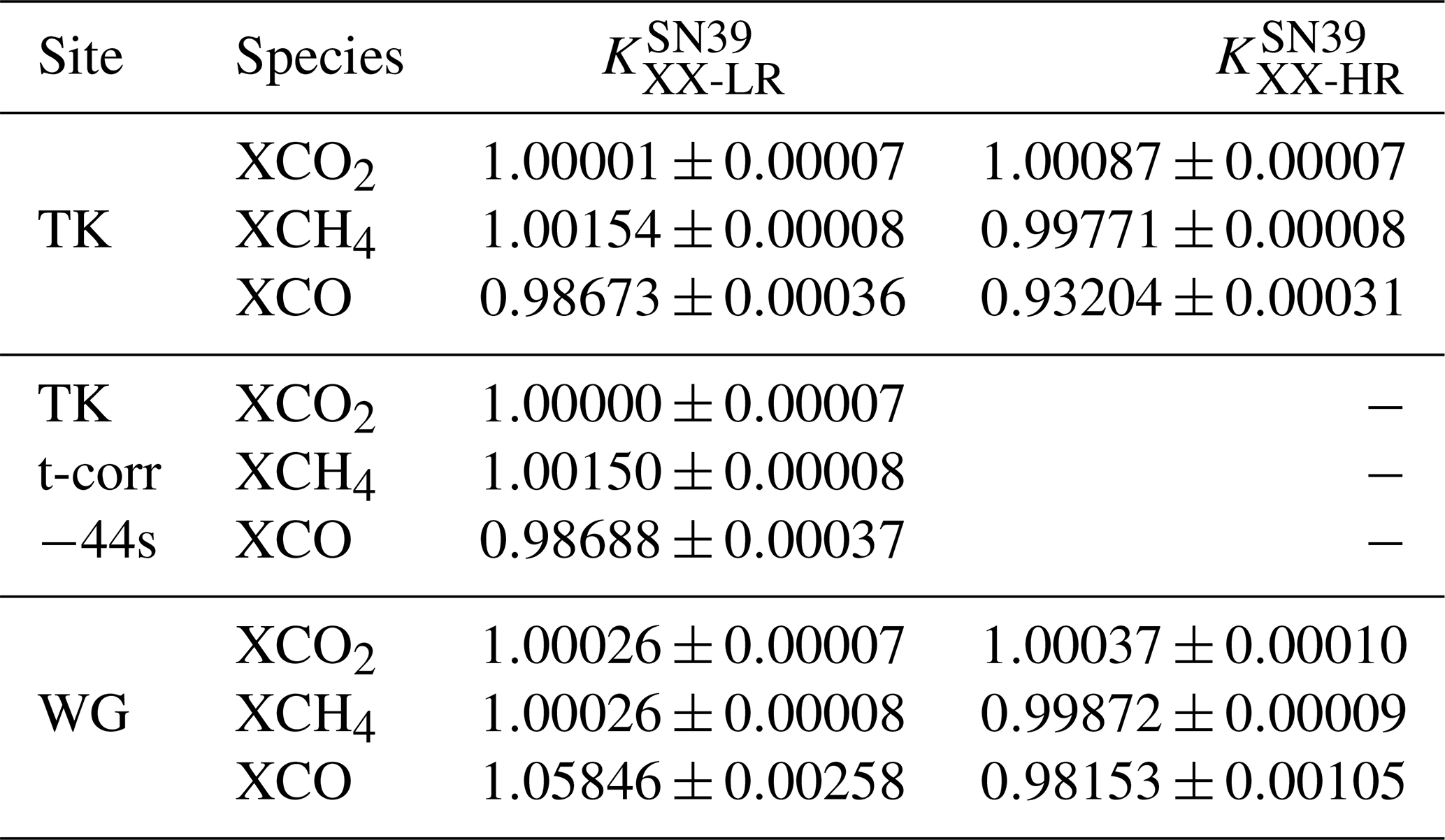
The “virtual” bias compensation factors comparing the visited TCCON sites to the reference in Karlsruhe are given in Table A2. Based on these numbers, the deviations in percentage which are given in Table 4 are calculated.

Table A2 The table shows the bias compensation factors between the visited TCCON sites and the Karlsruhe reference (SN37). All values are given with a random error followed by the calibration uncertainty. Both values are described in Sect. 7.2. Since the COCCON network as a whole is calibrated in a way that the reference spectrometer matches with the TCCON Karlsruhe data, a comparison with the COCCON reference spectrometer is equal to a comparison of the TCCON-Karlsruhe site.

Appendix B: Virtual bias compensation factors and their error analysis

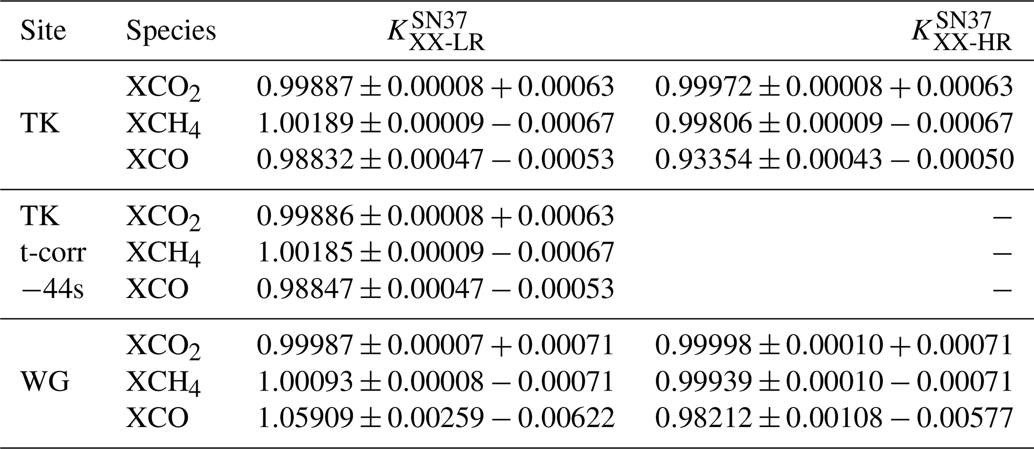
B1 Virtual bias compensation factors

The “virtual” bias compensation factors to compare the visited TCCON sites with the Karlsruhe reference are calculated by the multiplication of the factors between the TCCON site and the TS and the TS and the Karlsruhe reference:

$$\begin{array}{}\text{(B1)}& K_{\mathrm{TC}\text{-}\mathrm{ID}}^{\mathrm{TC}\text{-}\mathrm{KA}}=K_{\mathrm{TC}\text{-}\mathrm{ID}}^{\mathrm{TS}}\cdot K_{\mathrm{TS}}^{\mathrm{SN}\mathrm{37}}\cdot K_{\mathrm{SN}\mathrm{37}}^{\mathrm{TC}\text{-}\mathrm{KA}}.\end{array}$$

To calculate a deviation in percentage, first an offset in units of the column-averaged, dry air mole fraction is calculated. For this, the factors are multiplied by the average of the XGas over the whole period of a campaign $\stackrel{\mathrm{‾}}{{\text{XGas}}_{\mathrm{TC}\text{-}\mathrm{ID}}}$,

$$\begin{array}{}\text{(B2)}& \mathrm{\Delta }{\text{XGas}}_{\mathrm{TC}\text{-}\mathrm{ID}}^{\mathrm{TC}\text{-}\mathrm{KA}}={\stackrel{\mathrm{‾}}{\text{XGas}}}_{\mathrm{TC}\text{-}\mathrm{ID}}\left(\mathrm{1}-K_{\mathrm{TC}\text{-}\mathrm{ID}}^{\mathrm{TC}\text{-}\mathrm{KA}}\right).\end{array}$$

Using Eq. (B2), a deviation in percentage relative to the Karlsruhe TCCON site can be calculated using

$$\begin{array}{}\text{(B3)}& {\displaystyle }{\mathrm{\Delta }}_{\mathit{\%}}{\text{XGas}}_{\mathrm{TC}\text{-}\mathrm{ID}}^{\mathrm{TC}\text{-}\mathrm{KA}}={\displaystyle \frac{\mathrm{\Delta }{\text{XGas}}_{\mathrm{TC}\text{-}\mathrm{ID}}^{\mathrm{TC}\text{-}\mathrm{KA}}}{{\stackrel{\mathrm{‾}}{\text{XGas}}}_{\mathrm{TC}\text{-}\mathrm{KA}}}}\cdot \mathrm{100}\text{(B4)}& {\displaystyle }={\displaystyle \frac{\mathrm{1}-K_{\mathrm{TC}\text{-}\mathrm{ID}}^{\mathrm{TC}\text{-}\mathrm{KA}}}{K_{\mathrm{TC}\text{-}\mathrm{ID}}^{\mathrm{TC}\text{-}\mathrm{KA}}}}\cdot \mathrm{100},\end{array}$$

With ${\stackrel{\mathrm{‾}}{\text{XGas}}}_{\mathrm{TC}\text{-}\mathrm{KA}}={\stackrel{\mathrm{‾}}{\text{XGas}}}_{\mathrm{TC}\text{-}\mathrm{ID}}\cdot K_{\mathrm{TC}\text{-}\mathrm{ID}}^{\mathrm{TC}\text{-}\mathrm{KA}}$, the temporal mean of the KA data is expressed using the correction factors and the temporal mean of the corresponding site. Equation (B4) is used to calculate the deviations given in Table 4.

B2 Error analysis

In this section the details of the error analysis of the virtual bias compensation factors are carried out.

Random Error. The first part describes the propagation of the individual random errors described in Sect. A1 when multiplying different bias compensation factors. In this case, the random error of the resulting product is calculated using Gaussian error propagation, as described in Eq. (A4)

$$\begin{array}{}\text{(B5)}& {\displaystyle \frac{{\mathit{ϵ}}_{\mathrm{rand}}\left(K_{\mathrm{TC}\text{-}\mathrm{ID}}^{\mathrm{SN}\mathrm{37}}\right)}{K_{\mathrm{TC}\text{-}\mathrm{ID}}^{\mathrm{SN}\mathrm{37}}}}={\left[{\left({\displaystyle \frac{\mathit{ϵ}\left(K_{\mathrm{TC}\text{-}\mathrm{ID}}^{\mathrm{TS}}\right)}{K_{\mathrm{TC}\text{-}\mathrm{ID}}^{\mathrm{TS}}}}\right)}^{\mathrm{2}}+{\left({\displaystyle \frac{\mathit{ϵ}\left(K_{\mathrm{TS}}^{\mathrm{SN}\mathrm{37}}\right)}{K_{\mathrm{TS}}^{\mathrm{SN}\mathrm{37}}}}\right)}^{\mathrm{2}}\right]}^{\frac{\mathrm{1}}{\mathrm{2}}}.\end{array}$$

The errors described by Eq. (B5) are given in Table A2.

When calculating the deviation in percentage, as given in Table 4, the relative random error is calculated by

$$\begin{array}{}\text{(B6)}& \begin{array}{rl}& {\displaystyle \frac{{\mathit{ϵ}}_{\mathrm{rand}}\left({\mathrm{\Delta }}_{\mathit{\%}}\text{XGas}\right)}{{\mathrm{\Delta }}_{\mathit{\%}}\text{XGas}}}\\ & ={\left[{\left[{\displaystyle \frac{\partial }{\partial K_{\mathrm{TC}\text{-}\mathrm{ID}}^{\mathrm{SN}\mathrm{37}}}}\left({\mathrm{\Delta }}_{\mathit{\%}}{\text{XGas}}_{\mathrm{TC}\text{-}\mathrm{ID}}^{\mathrm{SN}\mathrm{37}}\right)\cdot {\displaystyle \frac{{\mathit{ϵ}}_{\mathrm{rand}}\left(K_{\mathrm{TC}\text{-}\mathrm{ID}}^{\mathrm{SN}\mathrm{37}}\right)}{K_{\mathrm{TC}\text{-}\mathrm{ID}}^{\mathrm{SN}\mathrm{37}}}}\right]}^{\mathrm{2}}\right]}^{\frac{\mathrm{1}}{\mathrm{2}}}\\ & ={\displaystyle \frac{\mathrm{1}}{{\left(K_{\mathrm{TC}\text{-}\mathrm{ID}}^{\mathrm{SN}\mathrm{37}}\right)}^{\mathrm{2}}}}\cdot {\displaystyle \frac{{\mathit{ϵ}}_{\mathrm{rand}}\left(K_{\mathrm{TC}\text{-}\mathrm{ID}}^{\mathrm{SN}\mathrm{37}}\right)}{K_{\mathrm{TC}\text{-}\mathrm{ID}}^{\mathrm{SN}\mathrm{37}}}}.\end{array}\end{array}$$

Calibration uncertainty. The second part is the uncertainty introduced by a potential drift of the TS instrument relative to the COCCON reference. Its upper limit is estimated by using the $\mathrm{\Delta }{K}_{\mathrm{SN}\mathrm{39}}^{\mathrm{SN}\mathrm{37}}$ of the bias compensation factors measured before and after each campaign as given in Table 1. Since $\mathrm{\Delta }{K}_{\mathrm{SN}\mathrm{39}}^{\mathrm{SN}\mathrm{37}}$ are values in percentage, the uncertainty of the final $K_{\mathrm{ID}\text{-}\mathrm{LR}/\mathrm{HR}}^{\mathrm{SN}\mathrm{37}}$ are calculated by

$$\begin{array}{}\text{(B7)}& {\mathit{ϵ}}_{\mathrm{calib}.}\left(K_{\mathrm{XX}\text{-}\mathrm{LR}/\mathrm{HR}}^{\mathrm{SN}\mathrm{37}}\right)=\mathrm{\Delta }{K}_{\mathrm{SN}\mathrm{39}}^{\mathrm{SN}\mathrm{37}}\cdot K_{\mathrm{XX}\text{-}\mathrm{LR}/\mathrm{HR}}^{\mathrm{SN}\mathrm{37}}\cdot {\displaystyle \frac{\mathrm{1}}{\mathrm{100}}}.\end{array}$$

In Table A2, the uncertainty is given as the second value.

For the deviation in percentage, the calibration uncertainty is calculated using linear error propagation of Eq. (B4) and using the error given in Eq. (B7):

$$\begin{array}{}\text{(B8)}& {\displaystyle }{\mathit{ϵ}}_{\mathrm{calib}.}\left({\mathrm{\Delta }}_{\mathit{\%}}\right)={\displaystyle \frac{\partial }{\partial K_{\mathrm{XX}}^{\mathrm{YY}}}}{\mathrm{\Delta }}_{\mathit{\%}}{\text{XGas}}_{\mathrm{XX}}^{\mathrm{YY}}\cdot \mathrm{\Delta }{K}_{\mathrm{XX}}^{\mathrm{YY}},\text{(B9)}& {\displaystyle }={\displaystyle \frac{-\mathrm{1}}{{\left(K_{\mathrm{XX}}^{\mathrm{YY}}\right)}^{\mathrm{2}}}}\cdot {\mathit{ϵ}}_{\mathrm{calib}}\left(K_{\mathrm{XX}\text{-}\mathrm{LR}/\mathrm{HR}}^{\mathrm{SN}\mathrm{37}}\right)\cdot \mathrm{100}.\end{array}$$

The result of this error analysis is given in Table 4. Here again, the random error is given first with a ± sign, and the calibration uncertainty is given second.

Appendix C: Raw data of Tsukuba with time correction

The air mass dependency of XAIR found in the Tsukuba TCCON data can be traced back to a wrong timestamp of the spectra. For the LR data, empirically it is found that an offset of −44 s can correct the air mass dependency. The corrected data are shown in Fig. C1. Note that this is not official TCCON data. For the TK-HR data, the timing error is currently under investigation. As soon as it is solved, the data will be submitted to TCCON.

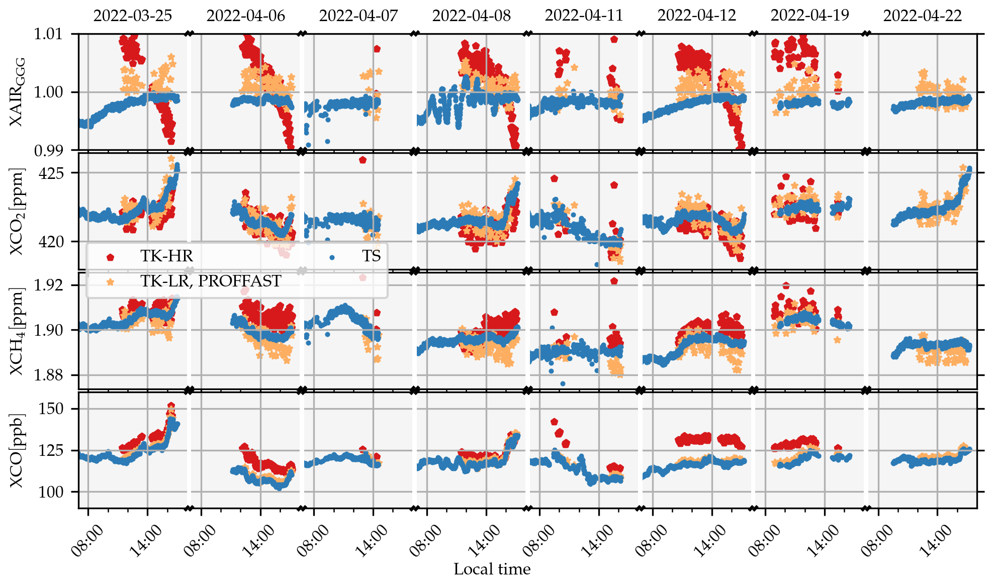
Figure C1 The XGas results for XCO₂, XCH₄ and XCO of the side-by-side measurements in Tsukuba, Japan with a time correction of −44 s for the LR data. This removes the time dependency. Note that the data shown here is no official TCCON data, as the time error is going to be corrected before publishing it. The subscript “GGG” at XAIR indicates that the XAIR values of PROFFAST are inverted to be comparable with the GGG XAIR values.

Appendix D: Pressure plots

In Figs. D1, D2, and D3 the comparison of the pressure measurements of the TCCON sites in Tsukuba, ETL and Wollongong with the TS using a Vaisala PTB330 and the TCCON pressure sensors are plotted. The data is discussed in the main text.

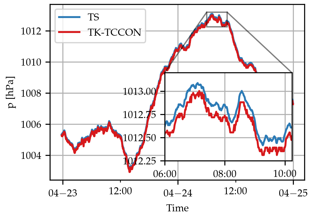
Figure D1 The pressure recorded at the Tsukuba TCCON site with the official TCCON sensor (TK) is plotted in red with the TS in blue. From the inset, one can see that there is a small difference of −0.105 hPa on average. This results in a bias compensation factor of $k_{{\mathrm{TK}}_{\mathrm{p}}}^{{\mathrm{TS}}_{\mathrm{p}}}=\mathrm{1.000104}$. For the comparison, the TS pressure sensor was placed side-by-side at the same height as the TK pressure sensor.

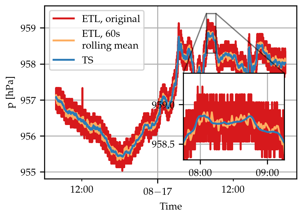
Figure D2 The pressure recorded at the ETL-TCCON site with the official TCCON sensor and the TS. The TCCON data show a high noise level. This is accounted for by taking the rolling mean with a window size of 60 s, plotted in orange. The original data are plotted in green. For the comparison, both the TS and the rolling mean data are resampled to 60 s bins. This yields a average deviation of −0.00419 hPa and a bias compensation factor of $k_{{\mathrm{ETL}}_{\mathrm{p}}}^{{\mathrm{TS}}_{\mathrm{p}}}=\mathrm{0.999996}$.

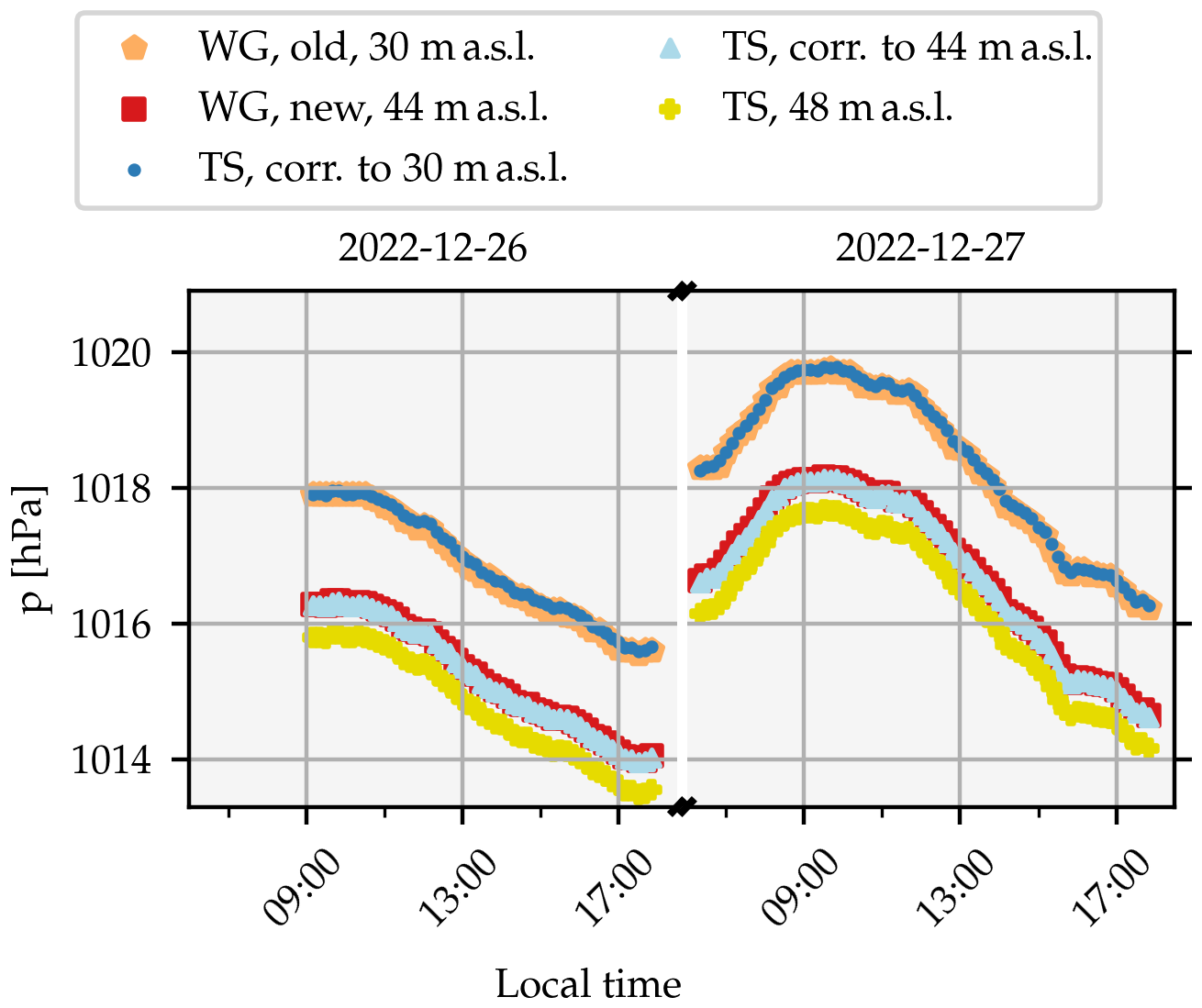
Figure D3 Pressure comparison for two exemplary days of the Wollongong pressure sensors and the TS. In WG, there is an old and a new TCCON spectrometer. The old one is the operable one, whereas the new one is still in the testing phase. Both are equipped with pressure sensors. The old sensor is at 30 m a.s.l.; the new one is at 44 m a.s.l. The TS measured at 48 m a.s.l. altitude; hence, its data are height corrected by −4 m (light blue triangles) and −18 m (blue dots). For both TCCON pressure sensors, the data are in good agreement with the height corrected TS data. On average the pressure sensors of the new and old TCCON site deviates by 0.02517 hPa and −0.03770 hPa relative to the TS pressure measurements height corrected by −4 and −18 m a.s.l. For the pressure sensor of the old TCCON site, this gives a pressure compensation factor of $K_{{\mathrm{WG}}_{\mathrm{p}}}^{\mathrm{TS}}=\mathrm{1.0000373}$. The shown days are chosen randomly; the numbers are calculated using the whole pressure record available.