Retrieval of aerosol optical depth over the Arctic cryosphere during spring and summer using satellite observations

The climate in the Arctic has warmed much more quickly in the last 2 to 3 decades than at the mid-latitudes, i.e., during the Arctic amplification (AA) period. Radiative forcing in the Arctic is influenced both directly and indirectly by aerosols. However, their observation from ground or airborne instruments is challenging, and thus measurements are sparse. In this study, total aerosol optical depth (AOD) is determined from top-of-atmosphere reflectance measurements by the Advanced Along-Track Scanning Radiometer (AATSR) on board ENVISAT over snow and ice in the Arctic using a retrieval called AEROSNOW for the period 2003 to 2011. AEROSNOW incorporates an existing aerosol retrieval algorithm with a cloud-masking algorithm, alongside a novel quality-flagging methodology specifically designed for implementation in the high Arctic region (≥ 72^∘ N). We use the dual-viewing capability of the AATSR instrument to accurately determine the contribution of aerosol to the reflection at the top of the atmosphere for observations over the bright surfaces of the cryosphere in the Arctic. The AOD is retrieved assuming that the surface reflectance observed by the satellite can be well parameterized by a bidirectional snow reflectance distribution function (BRDF). The spatial distribution of AOD shows that high values in spring (March, April, May) and lower values in summer (June, July, August) are observed. The AEROSNOW AOD values are consistent with those from collocated Aerosol Robotic Network (AERONET) measurements, with no systematic bias found as a function of time. The AEROSNOW AOD in the high Arctic was validated by comparison with ground-based measurements at the PEARL, OPAL, Hornsund, and Thule stations. The AEROSNOW AOD value is less than 0.15 on average, and the linear regression of AEROSNOW and AERONET total AOD yields a slope of 0.98, a Pearson correlation coefficient of R=0.86, and a root mean square error (RMSE) of =0.01 for the monthly scale in both spring and summer. The AEROSNOW observation of increased AOD values over the high Arctic cryosphere during spring confirms clearly that Arctic haze events were well captured by this dataset. In addition, the AEROSNOW AOD results provide a novel and unique total AOD data product for the springtime and summertime from 2003 to 2011. These AOD values, retrieved from spaceborne observation, provide a unique insight into the high Arctic cryospheric region at high spatial resolution and temporal coverage.

1 Introduction

The Arctic has experienced a significant increase in near-surface air temperatures over the past 3 decades, the rate of temperature increase being about 4 times larger than the global mean (Rantanen et al., 2022). This phenomenon is known as Arctic amplification (AA). The warming of the Arctic has increased the rate of melting of the Arctic cryosphere, e.g., glaciers, sea ice, and snow-covered surfaces. Processes thought to influence AA include the following: surface albedo feedback (Perovich and Polashenski, 2012), warm air intrusion (Boisvert et al., 2016), oceanic heat transport (Nummelin et al., 2017), cloud feedback (Kapsch et al., 2013; He et al., 2019; Middlemas et al., 2020), lapse rate feedback (Pithan and Mauritsen, 2014), and effects influencing biological and oceanic particle emission (Park et al., 2015; Campen et al., 2022).

Atmospheric aerosols are a collection of solid or liquid suspended particles that have both natural and anthropogenic sources. It is well known that changes in the scattering and absorption of incoming solar radiation by aerosols have a direct impact on climate change (Bond et al., 2013). Increases in aerosol result in more solar radiation being scattered back into space, and the atmosphere and surface are cooled. On the other hand, aerosols that absorb solar radiation warm the atmosphere and surface. Aerosols also act as both cloud condensation nuclei (CCN) and ice nuclei particles (INP), affecting the microphysical and radiative properties of clouds. In this way, aerosols also indirectly affect climate change (Twomey, 1977; Kaufman and Fraser, 1997; Hartmann et al., 2020). However, neither the contribution of aerosols to AA nor the effect of declining regional snow and ice on aerosol during the AA period is well understood (Im et al., 2021).

In this study, we use aerosol optical depth (AOD) as an optical measure of aerosol. It is valuable in the analysis of the impact of aerosols on the Arctic climate and vice versa. The retrieval of AOD is complicated by the seasonal changes in solar geometry, surface albedo, and meteorology (Mei et al., 2013, 2020a; Stapf et al., 2020). AOD is defined as the columnar integration of the aerosol extinction coefficient (the sum of the absorption and scattering coefficient).

The Arctic is vast, and the ground-based measurements of AOD are inevitably sparse. This has limited our understanding of the direct and indirect impacts of aerosols on AA and vice versa. Recently there have been some campaigns which have investigated different processes of relevance to aerosol sources and sinks in the Arctic, e.g., the Multidisciplinary drifting Observatory for the Study of Arctic Climate (MOSAiC) campaign (Mech et al., 2022), Arctic CLoud Observations Using airborne measurements during polar Day/Physical feedbacks of Arctic planetary boundary level Sea ice, Cloud and AerosoL (ACLOUD/PASCAL) (Wendisch et al., 2023), and Polar Airborne Measurements and Arctic Regional Climate Model Simulation Project (PAMARCMIPs) (Hoffmann et al., 2012; Nakoudi et al., 2018; Ohata et al., 2021). In addition, there are other site-based long-term aerosol measurement studies (Herber et al., 2002; Tomasi et al., 2007; Moschos et al., 2022; Schmale et al., 2022). However, these provide inadequate spatiotemporal representation of the Arctic region (Sand et al., 2017). The sparseness of AOD may explain, at least in part, the variations in AOD simulations from different climate models (Sand et al., 2017). Without a doubt, the lack of AOD measurements in the Arctic limits our knowledge about radiative forcing and Arctic warming in global and regional climate models (Goosse et al., 2018).

Further, AOD has been retrieved from the measurements of reflectance at the top of the atmosphere (TOA) made by passive satellite remote-sensing instruments over the Arctic but almost exclusively over snow- and ice-free areas, i.e., land and ocean. A few recent studies have used such AOD products (e.g., Glantz et al., 2014; Wu et al., 2016; Sand et al., 2017; Xian et al., 2022) over open-ocean and snow- and ice-free surfaces and make a valuable contribution to closing the data gap mentioned above. However, these AOD products are not suitable over the cryosphere due to an inadequate parameterization of the surface reflectance over residual snow- and ice-covered areas (Mei et al., 2020a) and Arctic cloud cover (Jafariserajehlou et al., 2019). In addition, typical illumination conditions, i.e., large solar zenith angles (SZAs), make the AOD retrieval used in the Arctic more challenging and lead potentially to a significant overestimation of AOD values (Mei et al., 2013).

Several dedicated algorithms for passive satellite remote sensing over snow and ice have been developed. Istomina et al. (2009) and later Mei et al. (2013, 2020a, b) provided valuable pioneering research. However, these attempts have mostly been confined to the island of Spitsbergen in the Svalbard archipelago in northern Norway. Thus far, there have been no attempts to systematically apply these algorithms together with the Arctic-adopted cloud-masking algorithm in the Arctic cryosphere to address the data gap identified above. Studies using active satellite remote sensing such as Sand et al. (2017) and Xian et al. (2022) are valuable, but the observational data are limited over the Arctic cryosphere.

With respect to using active satellite remote sensing, recently, Toth et al. (2018) and Xian et al. (2022) reported that the active satellite sensor, the Cloud-Aerosol Lidar with Orthogonal Polarization (CALIOP/CALIPSO) (Winker et al., 2004), has a significant fraction of aerosol profile data comprising retrieval fill values (−9999s or RFVs) and is thus rejected. This is partly due to the minimal detection limits of the lidar when measuring the signal scattered back into space. In fact, in some areas of the Arctic, over 80 % of CALIOP profiles consist entirely of RFVs (Toth et al., 2018; Xian et al., 2022).

The objective of this study is to retrieve the AOD over snow- and ice-covered regions of the Arctic by using passive remote sensing from space. We retrieve the total AOD using an approach first described by Istomina et al. (2009), which we have further integrated with the cloud-masking algorithm of Jafariserajehlou et al. (2019) and named AEROSNOW. This AEROSNOW approach was then systematically applied over vast Arctic cryospheric regions. We assessed the quality of AEROSNOW by using Aerosol Robotic Network (AERONET) measurements to validate the retrieved AOD. After retrieval and validation, we discuss the distribution of AOD over Arctic snow and ice in spring and summer, where ground-based and other spaceborne observational AOD data are limited. The purpose of examining these distributions is to gain further confidence in this new dataset and to investigate the distributions with respect to our expectations. We examine whether the AOD retrieved by AEROSNOW is able to capture increased levels of AOD in spring compared to summer (Willis et al., 2018), which would be a confirmation of whether or not AEROSNOW is able to track Arctic haze events.

We have generated the AEROSNOW AOD dataset for the period from 2003 to 2011 (9 years). The algorithm uses the measurements made by the Advanced Along-Track Scanning Radiometer (AATSR) over the Arctic. A short description of the AATSR data and the corresponding retrieval is given in Sect. 2, and the description of the AEROSNOW algorithm is given in Sect. 3. To determine the quality of the AEROSNOW datasets, we compare them with accurate ground-based AERONET measurements in the high Arctic. The description of the AERONET dataset is found in Sect. 2.3. The AERONET and AEROSNOW values are then compared over snow- and ice-covered surfaces in Sect. 4. Finally, we draw conclusions in Sect. 5.

2 Datasets

To investigate the distribution and variability of Arctic aerosols over snow and ice, we have employed passive remote sensing during spring (March, April, May – MAM) and summer (June, July, August – JJA), which is the time when the Arctic is illuminated by solar radiation.

Prior to the use of an AOD retrieval algorithm suitable for the Arctic, we necessitate a precise masking scheme adapted to Arctic cloud cover. After identifying cloud-free scenes, we applied the AOD retrieval algorithm. To create such an AOD retrieval framework suitable for the Arctic, we integrate two pioneering approaches, which we briefly summarize in the following sections. For cloud masking, we utilized the approach of Jafariserajehlou et al. (2019) (Sect. 3.1.1), and for AOD retrieval, we used Istomina et al. (2009) (Sect. 3.1.2). The integrated framework and the subsequent quality-flagging (QF) scheme are described in Sect. 3.2, which we have entitled AEROSNOW.

The AEROSNOW algorithm is applied to the dual-viewing Level-1B data product reflectance at the top of the atmosphere made by the AATSR (Llewellyn-Jones and Remedios, 2012). We have validated the AEROSNOW-retrieved AOD by comparing it with the AOD measured by the ground-based sun-photometer measurements, AERONET (Holben et al., 1998). In addition, the use of validation sources other than AERONET would have been very helpful. Unfortunately, data from valuable campaigns and expeditions such as POLAR-AOD (Mazzola et al., 2012), MOSAiC expedition and MOSAiC-ACA (Mech et al., 2022), and AFLUX/PASCAL – Arctic (Mech et al., 2022) were only available after 2011. For this reason, we have focused on validation with ground-based AERONET measurements. We introduce AATSR and AERONET data in Sect. 2.1 and 2.3, respectively.

2.1 Spaceborne observation: AATSR instrument

AATSR flew as part of the payload of the European Space Agency's (ESA's) ENVISAT, which was launched on 28 February 2002 and failed on 8 April 2012. ENVISAT flew in a sun-synchronous orbit with an Equator-crossing local time of 10:00 mean local solar time (MLST). AATSR made measurements from May 2002 to April 2012. The spatial resolution of the AATSR observation data was 1 km at nadir. The swath width of AATSR was 512 km. AATSR had a dual-viewing capability with a forward-viewing angle of 55^∘. It made simultaneous measurements of the upwelling reflectances at wavelengths from the visible to the thermal infrared (0.55, 0.66, 0.87, 1.6, 3.7, 11, and 12 µm).

2.2 Spaceborne observation: MODIS cloud products

The Moderate Resolution Imaging Spectroradiometer (MODIS) is a sophisticated 36-channel passive-imaging sensor incorporated into the Terra (2000) and Aqua (2002) polar satellites. Featuring a substantial swath width of 2330 km, MODIS facilitates global coverage once or twice daily. Renowned for its precise onboard calibration mechanisms, MODIS sensors exhibit noteworthy calibration accuracy, as validated by Stubenrauch et al. (2013) and Stengel et al. (2017). The extensive cloud datasets derived from these sensors span over a decade, proving invaluable for climate studies. Prominent among these cloud climate data records (CDRs) are the Level-2 MODIS Global Product data files as detailed by Marchant et al. (2020). Additionally, the Clouds and the Earth's Radiant Energy System (CERES) Single Scanner Footprint (SSF) products, including CERES-SSF Terra and CERES-SSF Aqua, as outlined by Minnis et al. (2011), are frequently employed. Moreover, the Cloud Climate Change Initiative (Cloud cci) for MODIS data encompasses Cloud cci MODIS Terra and Cloud cci MODIS Aqua, as described by McGarragh et al. (2018) and Sus et al. (2018).

2.3 Ground-based measurements: AERONET Level-2 aerosol product

AERONET is a federated network of ground-based global sun photometers measuring solar and sky irradiance at various wavelengths from the near-ultraviolet to the near-infrared with high accuracy (Holben et al., 2001; Giles et al., 2019). AERONET sun photometers record AOD values every 15 min in typically seven spectral channels (nominally 340, 380, 440, 500, 670, 870, and 1020 nm) (Holben et al., 2001). The quality-assured AERONET version 3 Level-2 data are used in this study (accessed at https://aeronet.gsfc.nasa.gov/, last access: 3 February 2022).

The AOD values from AERONET stations in the high Arctic were used to assess the data quality of AOD estimated using AEROSNOW. The names and locations of the AERONET stations selected are PEARL (80.054^∘ N, 86.417^∘ W), OPAL (79.990^∘ N, 85.939^∘ W), Hornsund (77.001^∘ N, 15.540^∘ E), and Thule (76.516^∘ N, 68.769^∘ W) and are shown in Fig. 1. Two sites are located over the Canadian archipelago (CA), which typically has aerosol of natural origin (Breider et al., 2017), and one station (Hornsund) is on Spitsbergen, which is known to be affected by polluted air masses transported from lower latitudes.

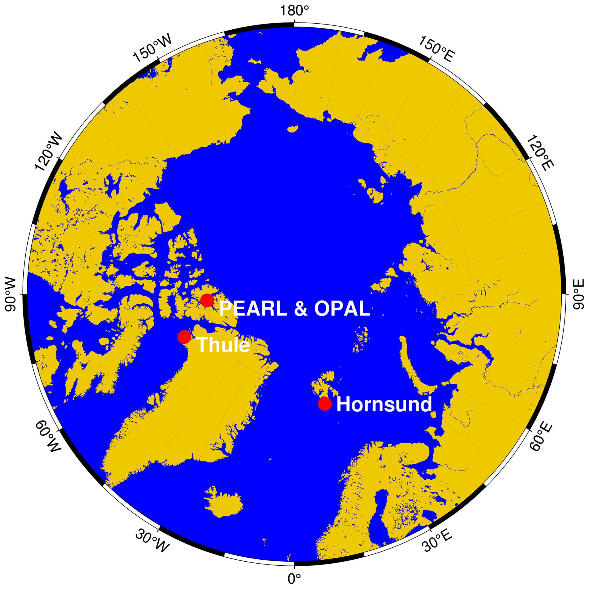
Figure 1 Locations of the PEARL, OPAL, Hornsund, and Thule AERONET measurement stations considered in this study.

3 Methodology: AEROSNOW development

The dual-viewing capability of the AATSR instrument was used to retrieve AOD over the pan-Arctic snow and ice region. Before an AOD retrieval algorithm suitable for the Arctic can be used, we need a rigorous Arctic-adopted cloud detection algorithm. Therefore, in this study, we developed the AEROSNOW framework for pan-Arctic AOD retrieval. The core development of AEROSNOW involves the integration of two different algorithms. The first algorithm is the cloud detection algorithm of Jafariserajehlou et al. published in 2019, which is described in Sect. 3.1.1, with the core AOD retrieval algorithm of Istomina et al. published in 2009, which is described in Sect. 3.1.2, followed by the quality flagging described in the following Sect. 3.2.

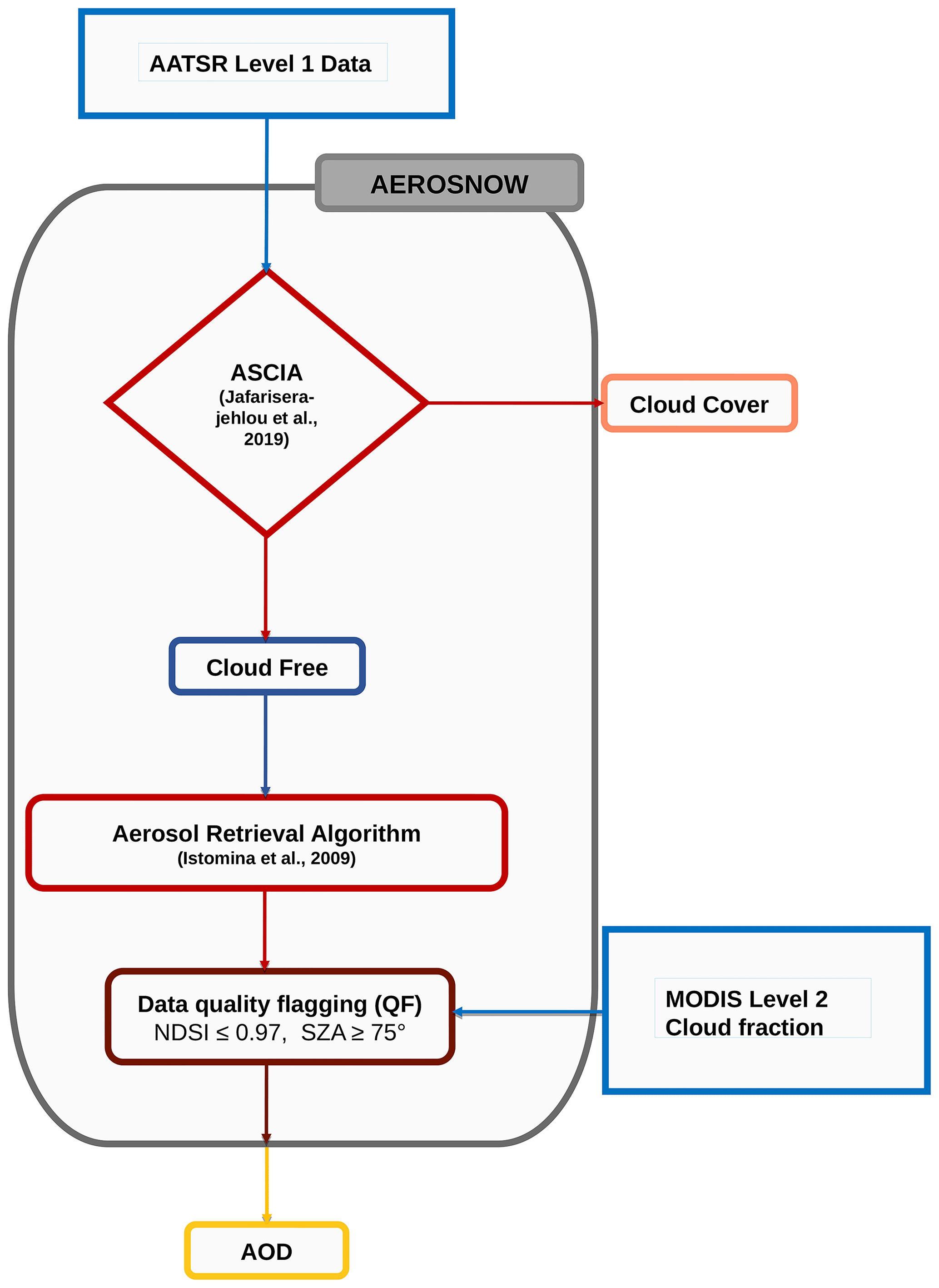
After formulating the AEROSNOW framework, we applied it systematically for the first time to the pan-Arctic cryosphere region to obtain spaceborne observational data with high spatial and temporal coverage. The flowchart describes the important building blocks of AEROSNOW presented in Fig. 2.

Figure 2 Flowchart describing the important building blocks of the AEROSNOW scheme.

3.1 The heritage of the cloud-masking and AOD retrieval algorithms

The heritage of the algorithms used in this study, such as the cloud identification algorithm (Jafariserajehlou et al., 2019) and the aerosol retrieval algorithm (Istomina et al., 2009), comes from earlier studies made at the Institute of Environmental Physics of the University of Bremen.

3.1.1 Cloud detection algorithm

The cloud detection algorithm used in AEROSNOW is discussed in Jafariserajehlou et al. (2019). The AATSR–Sea and Land Surface Temperature Radiometer (SLSTR) cloud identification algorithm (ASCIA) was developed to address the requirements of Arctic cloud identification. The ASCIA is explained in more detail in Jafariserajehlou et al. (2019). Briefly, the ASCIA combines two approaches to detect the presence of clouds: (i) a Pearson correlation coefficient (PCC) analysis of the reflectance at the TOA at 1.6 µm wavelength and (ii) the use of the reflectance at the TOA for a wavelength of 3.7 µm. The PCC analysis separates the reflectance of the surface from cloud reflectance at the TOA. The surface reflectance is stable, while the cloud reflectance at the TOA is highly variable over a short period of time. The PCC for two satellite scenes, such as x and y, is a function of their covariance normalized by their standard deviations (Benesty et al., 2009). It can be interpreted as a measure of how well these two satellite scenes are correlated. (Lyapustin et al., 2008).

$$\begin{array}{}\text{(1)}& \mathrm{\text{PCC}}={\displaystyle \frac{\text{COV}(x,y)}{{\mathit{\sigma }}_x{\mathit{\sigma }}_y}},\text{COV}(x,y)={\displaystyle \frac{\mathrm{1}}{N}}\sum _{i=\mathrm{1}}^N\left(x_i-\stackrel{\mathrm{‾}}{x}\left)\right(y_i-\stackrel{\mathrm{‾}}{y}\right)\end{array}$$

COV(x,y) is the covariance of variables x and y, and σ is the standard deviation of each variable.

$$\begin{array}{}\text{(2)}& {\mathit{\sigma }}_x=\sqrt{{\displaystyle \frac{\mathrm{1}}{N}}\sum _{i=\mathrm{1}}^N{\left(x_i-\stackrel{\mathrm{‾}}{x}\right)}^{\mathrm{2}}},{\mathit{\sigma }}_y=\sqrt{{\displaystyle \frac{\mathrm{1}}{N}}\sum _{j=\mathrm{1}}^N{\left(y_j-\stackrel{\mathrm{‾}}{x}\right)}^{\mathrm{2}}}\end{array}$$

The mean values of x and y are $\stackrel{\mathrm{‾}}{x}$ and $\stackrel{\mathrm{‾}}{y}$, respectively. The PCC has values between −1 and +1. The correlation or anticorrelation between the two variables is strongest when the absolute value is closer to 1 or −1, respectively. Consequently, the PCC values are derived using sets of reflectances at the TOA of the same area at different times, which give an indication of whether the scene is cloudy or cloud-free (Lyapustin et al., 2008). The PCC is calculated individually for areas of 25 km × 25 km. Based on statistical analysis, Jafariserajehlou et al. (2019) found a threshold of PCC ≤0.6 as a reliable value for the detection of mid-latitude clouds. This value is also in good agreement with a similar analysis by Lyapustin et al. (2008) using 1 year of MODIS data for 156 global AERONET stations, where they derived cutoff values of 0.65 to 0.68. In the Arctic, and especially over the cryosphere, surfaces are often found that have low visible or thermal contrast compared to mid-latitudes. Thus, a specific analysis in the Arctic was performed by Jafariserajehlou et al. (2019) to account for reduced structural patterns due to frequent snow or ice cover. They determined a threshold of PCC ≥0.4 for cloud-free scenes in the Arctic. Having selected cloud-free ground scenes using the PCC on the 25 km × 25 km scale, Jafariserajehlou et al. (2019) introduced an additional criterion using the reflectance at 3.7 µm. They used this channel because the single scattering albedo at 3.7 µm, compared to that in the visible (VIS) and near-infrared (NIR) wavelength ranges, is more sensitive to the absorption of liquid water, ice, or snow (Platnick and Fontenla, 2008).

In summary, a PCC analysis at the 25 km × 25 km scale is performed to identify cloudy and cloud-free scenes that are assumed to have low and high PCC values, respectively. The results of this step are binary flags at the 25 km × 25 km scale. This serves as input to the second step of the algorithm, where the reflectance at the TOA for 3.7 µm is used to create binary flags at 1 km × 1 km (AATSR spatial resolution of the instrument at nadir) to identify clouds. The combination of these two constraints is necessary because neither the PCC analysis nor the reflectance of the 3.7 µm channel alone is sufficient for accurate cloud identification in the Arctic (Jafariserajehlou et al., 2019).

At the 3.7 µm channel, the reflectance of the snow or ice surface (0.005–0.025) has interference with those of ice clouds (0.01–0.3). To avoid the uncertainty arising from this interference, Jafariserajehlou et al. (2019) optimized ASCIA by using thresholds as follows.

• i.

  An area of 25 km × 25 km with PCC ≥0.4 is then further analyzed on the pixel level (1 km × 1 km) by using the reflectance at the TOA at 3.7 µm. A scene is considered cloud-free if the TOA reflectance at 3.7 µm is larger than 0.04, following Allen et al. (1990).

• ii.

  If an area of 25 km × 25 km has a value of PCC <0.4 and the TOA reflectance at 3.7 µm for the pixel (1 km × 1 km) level is less than 0.015, the pixel is considered to be cloudy. This threshold is equal to or lower than the lowest observed reflectance of ice clouds at 3.7 µm (Allen et al., 1990).

For more information, the reader is referred to the schematic flowchart of the cloud identification algorithm shown in Fig. 4 of the article by Jafariserajehlou et al. (2019).

In the ASCIA study, the areas identified as cloud-free are assumed to be unchanged for the sampling period of ±30 min, while cloudy or partly cloudy scenes exhibit much greater spatial and temporal variability. The cloud fraction retrieved by ASCIA has been validated with surface synoptic observations (SYNOP) (WMO, 1995) ground-based cloud fraction measurements made during the period of the AATSR (2003 to 2011) and the SLSTR (2018). The World Meteorological Organization (WMO) established SYNOP stations for weather information around the world. The locations of the SYNOP stations used for the ASCIA validation within the Arctic Circle are shown in Fig. 3 of Jafariserajehlou et al. (2019). The okta scale is used to report the SYNOP cloud fraction. The discrete okta values range from 0 (completely clear sky) to 8 (completely obscured by clouds). The usual assumption is that 1 okta equals 12.5 % of cloud coverage. The ASCIA study follows Boers et al. (2010), suggesting a larger range of 18.75 % for 1 okta. The use of the okta measurements in ASCIA required the estimation of the error or uncertainty in the measurements. In Boers et al. (2010) and Werkmeister et al. (2015), the SYNOP cloudiness okta estimation has errors of ±1 okta for values of okta between 1 and 7 and a value of ±2 okta for 0 or 8 okta.

The ASCIA cloud detection algorithm achieved promising agreements of more than 95 % and 83 % within ±2 and ±1 okta when compared with ground-based synoptic surface observations (SYNOP) (WMO, 1995) over the Arctic. In general, ASCIA shows a better performance in detecting clouds over Arctic ground scenes than other algorithms applied to AATSR measurements.

3.1.2 AOD retrieval algorithm

The approach used in our retrieval algorithm was first discussed in Istomina et al. (2009). The reflectance at the TOA, as shown by Chandrasekhar (1950) and Kaufman et al. (1997), is given as follows.

$$\begin{array}{}\text{(3)}& \begin{array}{rl}{\mathit{\rho }}_{\mathrm{TOA}}\left(\mathit{\lambda },{\mathit{\mu }}_{\mathrm{0}},\mathit{\mu },\mathit{\varphi },\mathit{\tau }\right)& ={\mathit{\rho }}_{\mathrm{atm}}\left(\mathit{\lambda },{\mathit{\mu }}_{\mathrm{0}},\mathit{\mu },\mathit{\varphi },\mathit{\tau }\right)\\ & +{\displaystyle \frac{A_{\mathrm{sfc}}\left(\mathit{\lambda }\right)T_{\mathrm{1}}\left(\mathit{\lambda },{\mathit{\mu }}_{\mathrm{0}},\mathit{\tau }\right)T_{\mathrm{2}}\left(\mathit{\lambda },\mathit{\mu },\mathit{\tau }\right)}{\mathrm{1}-A_{\mathrm{sfc}}\left(\mathit{\lambda }\right)s\left(\mathit{\lambda }\right)}}\end{array}\end{array}$$

μ=cos θ and μ₀=cos θ₀, θ₀, and θ are the solar zenith angle and the zenith angle, respectively, of the satellite; ϕ is the relative azimuth angle; λ is the wavelength; and ${\mathit{\rho }}_{\mathrm{TOA}}(\mathit{\lambda },{\mathit{\mu }}_{\mathrm{0}},\mathit{\mu },\mathit{\varphi },\mathit{\tau })$ is the satellite-measured TOA reflectance. ${\mathit{\rho }}_{\mathrm{atm}}(\mathit{\lambda },{\mathit{\mu }}_{\mathrm{0}},\mathit{\mu },\mathit{\varphi },\mathit{\tau })$ is the contribution of atmospheric reflectance to TOA reflectance, A_sfc(λ) is the surface spectral albedo, $T_{\mathrm{1}}(\mathit{\lambda },{\mathit{\mu }}_{\mathrm{0}},\mathit{\tau })$ is the downward transmission of light, $T_{\mathrm{2}}(\mathit{\lambda },\mathit{\mu },\mathit{\tau })$ is the surface-to-TOA transmission of light, and s(λ) is the atmospheric hemispherical albedo. The separation of the various effects contributing to TOA reflectance is the mathematical problem to be solved. This was achieved by using the BRDF of the snow reflectance.

As suggested by Flowerdew and Haigh (1995), the surface reflectance can be approximated by two terms, one term describing the variation in wavelength and another describing the variation in geometry. To a first approximation, the ratio between the surface reflectances at two viewing angles depends only on the wavelength. This principle has already been successfully applied in the AATSR-DV algorithm (Veefkind et al., 1998; Curier et al., 2009). Furthermore, Vermote et al. (1997) determined the ratio between the estimated BRDF and the actual surface BRDF for the atmospheric correction and mentioned that this ratio is only affected by the shape of the BRDF and not by its magnitude. This means that the effect of the surface reflection can be eliminated by using the ratio of AATSR dual-viewing observations measured in the forward and nadir views (Veefkind et al., 1998; Istomina et al., 2009, 2011).

By assuming that a Lambertian surface A_sfc(λ) is equal to the surface reflectance ρ_sfc(λ) using Eq. (3), we obtain the following.

$$\begin{array}{}\text{(4)}& \begin{array}{rl}& {\displaystyle \frac{{\mathit{\rho }}_{\mathrm{sfc}}^{\mathrm{f}}(\mathit{\lambda },{\mathit{\mu }}_{\mathrm{0}},\mathit{\mu },\mathit{\varphi })}{{\mathit{\rho }}_{\mathrm{sfc}}^{\mathrm{n}}(\mathit{\lambda },{\mathit{\mu }}_{\mathrm{0}},\mathit{\mu },\mathit{\varphi })}}\\ & ={\displaystyle \frac{{\mathit{\rho }}_{\mathrm{TOA}}^{\mathrm{f}}(\mathit{\lambda },{\mathit{\mu }}_{\mathrm{0}},\mathit{\mu },\mathit{\varphi },\mathit{\tau })-{\mathit{\rho }}_{\mathrm{atm}}^{\mathrm{f}}(\mathit{\lambda },{\mathit{\mu }}_{\mathrm{0}},\mathit{\mu },\mathit{\varphi },\mathit{\tau })}{{\mathit{\rho }}_{\mathrm{TOA}}^n(\mathit{\lambda },{\mathit{\mu }}_{\mathrm{0}},\mathit{\mu },\mathit{\varphi },\mathit{\tau })-{\mathit{\rho }}_{\mathrm{atm}}^{\mathrm{n}}(\mathit{\lambda },{\mathit{\mu }}_{\mathrm{0}},\mathit{\mu },\mathit{\varphi },\mathit{\tau })}}\\ & \cdot {\displaystyle \frac{T^{\mathrm{n}}(\mathit{\lambda },\mathit{\mu },\mathit{\tau })}{T^{\mathrm{f}}(\mathit{\lambda },\mathit{\mu },\mathit{\tau })}}\end{array}\end{array}$$

${\mathit{\rho }}_{\mathrm{sfc}}(\mathit{\lambda },{\mathit{\mu }}_{\mathrm{0}},\mathit{\mu },\mathit{\varphi })$ is the reflectance from the surface, $T(\mathit{\lambda },\mathit{\mu },\mathit{\tau })=T_{\mathrm{1}}(\mathit{\lambda },{\mathit{\mu }}_{\mathrm{0}},\mathit{\tau })T_{\mathrm{2}}(\mathit{\lambda },\mathit{\mu },\mathit{\tau })$ is the total atmospheric transmittance from the surface to a satellite sensor, and f and n indicate the AATSR forward and nadir observation angles, respectively.

The left-hand-side term of Eq. (4) is a BRDF ratio. For the estimation of this ratio, the two-parameter snow BRDF model (Kokhanovsky and Breon, 2012) has been used to parameterize the snow spectral reflection function ${\mathit{\rho }}_{\mathrm{sfc}}(\mathit{\mu },{\mathit{\mu }}_{\mathrm{0}},\mathit{\varphi })$:

$$\begin{array}{}\text{(5)}& \begin{array}{rl}& {\mathit{\rho }}_{\mathrm{sfc}}(\mathit{\mu },{\mathit{\mu }}_{\mathrm{0}},\mathit{\varphi })\\ & ={\mathit{\rho }}_{\mathrm{0}}(\mathit{\mu },{\mathit{\mu }}_{\mathrm{0}},\mathit{\varphi })\times e^{[-\mathit{\psi }{K}_{\mathrm{0}}(\mathit{\mu }\left)K_{\mathrm{0}}\right({\mathit{\mu }}_{\mathrm{0}})/{\mathit{\rho }}_{\mathrm{0}}(\mathit{\mu },{\mathit{\mu }}_{\mathrm{0}},\mathit{\varphi }\left)\right]},\end{array}\end{array}$$

$$\begin{array}{}\text{(6)}& {\mathit{\rho }}_{\mathrm{0}}(\mathit{\mu },{\mathit{\mu }}_{\mathrm{0}},\mathit{\varphi })={\displaystyle \frac{a+b(\mathit{\mu }+{\mathit{\mu }}_{\mathrm{0}})+c\mathit{\mu }{\mathit{\mu }}_{\mathrm{0}}+p\left(\mathit{\theta }\right)}{\mathrm{4}(\mathit{\mu }+{\mathit{\mu }}_{\mathrm{0}})}},\end{array}$$

where

$$\begin{array}{}\text{(7)}& {\displaystyle }\begin{array}{rl}& K_{\mathrm{0}}\left(\mathit{\mu }\right)={\displaystyle \frac{\mathrm{3}}{\mathrm{7}}}(\mathrm{1}+\mathrm{2}\mathit{\mu }),K_{\mathrm{0}}\left({\mathit{\mu }}_{\mathrm{0}}\right)={\displaystyle \frac{\mathrm{3}}{\mathrm{7}}}(\mathrm{1}+\mathrm{2}{\mathit{\mu }}_{\mathrm{0}});\\ & a=\mathrm{1.247},b=\mathrm{1.186},c=\mathrm{5.157},\end{array}\text{(8)}& {\displaystyle }\begin{array}{rl}& p\left(\mathit{\theta }\right)=\mathrm{11.1}\exp (-\mathrm{0.087}\mathit{\theta })+\mathrm{1.1}\exp (-\mathrm{0.014}\mathit{\theta });\\ & \cos \mathit{\theta }=-\mathit{\mu }{\mathit{\mu }}_{\mathrm{0}}+s{s}_{\mathrm{0}}\cos \mathit{\varphi },\end{array}\text{(9)}& {\displaystyle }s=\sqrt{\mathrm{1}-{\mathit{\mu }}^{\mathrm{2}}},s_{\mathrm{0}}=\sqrt{\mathrm{1}-{\mathit{\mu }}_{\mathrm{0}}^{\mathrm{2}}}\mathit{\psi }=\sqrt{\mathit{\gamma }L}.\end{array}$$

$\mathit{\gamma }=\mathrm{4}\mathit{\pi }\times (\mathit{\chi }+M)\times {\mathit{\lambda }}^{-\mathrm{1}}$, χ is the imaginary part of the refractive index of ice, λ is the wavelength, L is related to the snow grain size, and M is related to the estimation of the absorption of light by pollutants (Kokhanovsky and Breon, 2012).

In order to take the snow structure into account, only a pure snow-covered area (100 % snow cover) is used for the retrieval. The Normalized Difference Snow Index (NDSI) is defined as the following.

$$\begin{array}{}\text{(10)}& \text{NDSI}={\displaystyle \frac{{\mathit{\rho }}_{\mathrm{0.55}}-{\mathit{\rho }}_{\mathrm{1.6}}}{{\mathit{\rho }}_{\mathrm{0.55}}+{\mathit{\rho }}_{\mathrm{1.6}}}}\end{array}$$

The NDSI is an index that refers to the presence of snow in a pixel and is a more accurate description of snow detection compared to fractional snow cover. Snow typically has a very high reflectance in the visible spectrum and a very low reflectance in the shortwave infrared (SWIR).

The BRDF model is analytical and has been compared with a set of multispectral and multidirectional measurements from the POLDER-3 (Polarization and Directionality of the Earth's Reflectances) instrument on board the PARASOL (Polarization and Anisotropy of Reflectances for Atmospheric Sciences coupled with Observations from a Lidar) satellite. Istomina et al. (2009) fixed the free parameters for the entire time series of the AATSR, which involved a fixed snow grain size and snow impurity assumptions. The BRDF model reproduces the directional variations in the measured reflectance with a root mean square error (RMSE) that is typically 0.005 in the visible wavelength range (Kokhanovsky and Breon, 2012), but the accuracy of the BRDF ratio is sufficient to retrieve aerosols. Accordingly, Istomina et al. (2009) assume that they can accurately estimate the BRDF ratio using Eqs. (3) to (9).

Similarly to Kokhanovsky and Schreier (2009), Istomina et al. (2009) assumed that the variability of ${\mathit{\rho }}_{\mathrm{atm}}(\mathit{\lambda },{\mathit{\mu }}_{\mathrm{0}},\mathit{\mu },\mathit{\varphi },\mathit{\tau })$ is small for different observational and solar illumination conditions in the Arctic. The simulations were done using the Arctic haze-phase function shown in Fig. 3 (Istomina et al., 2009). Two types of aerosol-phase functions were used in these simulations: Arctic haze and background aerosol. In Fig. 3, the phase functions for these two types are shown.

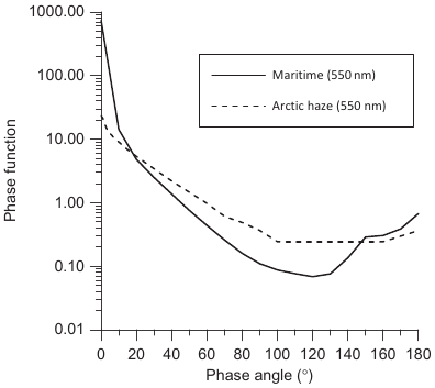
Figure 3 Phase function from ground-based measurement at 0.55 µm during the Arctic haze event on 23 March 2003 at Spitsbergen (78.923^∘ N, 11.923^∘ E) (Istomina et al., 2009). For comparison, the phase function for maritime aerosol is also shown.

Given the large solar zenith angle prevalent in the Arctic region, it becomes imperative to incorporate an air mass correction into the BRDF calculation, as the latter is intricately linked to the solar zenith angle. In this context, we employ the air mass factor as delineated by Kasten and Young (1989).

In Istomina et al. (2009), aerosol optical depth is derived using Eq. (4) and an iterative procedure involving observations at wavelength 555 nm. The following cost function 𝒞 is defined:

$$\begin{array}{}\text{(11)}& \begin{array}{rl}& \mathcal{C}=R\left(\mathit{\lambda },{\mathit{\mu }}_{\mathrm{0}},\mathit{\mu },\mathit{\varphi },\mathit{\tau }\right)\\ & -{\displaystyle \frac{{\mathit{\rho }}_{\mathrm{TOA},\mathrm{meas}}^{\mathrm{f}}-{\mathit{\rho }}_{\mathrm{atm},\mathrm{sim}}^{\mathrm{f}}\left(\mathit{\lambda },{\mathit{\mu }}_{\mathrm{0}},\mathit{\mu },\mathit{\varphi },\mathit{\tau }\right)T_{\mathrm{sim}}^{\mathrm{n}}\left(\mathit{\lambda },\mathit{\mu },\mathit{\tau }\right)}{{\mathit{\rho }}_{\mathrm{TOA},\mathrm{meas}}^{\mathrm{n}}-{\mathit{\rho }}_{\mathrm{atm},\mathrm{sim}}^{\mathrm{n}}\left(\mathit{\lambda },{\mathit{\mu }}_{\mathrm{0}},\mathit{\mu },\mathit{\varphi },\mathit{\tau }\right)T_{\mathrm{sim}}^{\mathrm{f}}\left(\mathit{\lambda },\mathit{\mu },\mathit{\tau }\right)}},\end{array}\end{array}$$

where

$$\begin{array}{}\text{(12)}& \begin{array}{rl}& R(\mathit{\lambda },{\mathit{\mu }}_{\mathrm{0}},\mathit{\mu },\mathit{\varphi },\mathit{\tau })\\ & ={\displaystyle \frac{{\mathit{\rho }}_{\mathrm{sfc},\mathrm{sim}}^{\mathrm{f}}(\mathit{\lambda },{\mathit{\mu }}_{\mathrm{0}},\mathit{\mu },\mathit{\varphi })}{{\mathit{\rho }}_{\mathrm{sfc},\mathrm{sim}}^{\mathrm{n}}(\mathit{\lambda },{\mathit{\mu }}_{\mathrm{0}},\mathit{\mu },\mathit{\varphi })}}{\displaystyle \frac{{\mathit{\rho }}_{\mathrm{TOA},\mathrm{sim}}^{\mathrm{n}}(\mathit{\lambda },{\mathit{\mu }}_{\mathrm{0}},\mathit{\mu },\mathit{\varphi },\mathit{\tau })}{{\mathit{\rho }}_{\mathrm{TOA},\mathrm{sim}}^{\mathrm{f}}(\mathit{\lambda },{\mathit{\mu }}_{\mathrm{0}},\mathit{\mu },\mathit{\varphi },\mathit{\tau })}}{\displaystyle \frac{{\mathit{\rho }}_{\mathrm{TOA},\mathrm{meas}}^{\mathrm{f}}}{{\mathit{\rho }}_{\mathrm{TOA},\mathrm{meas}}^{\mathrm{n}}}},\end{array}\end{array}$$

where ρ_TOA,meas is measured TOA reflectance, ${\mathit{\rho }}_{\mathrm{atm},\mathrm{sim}}(\mathit{\lambda },{\mathit{\mu }}_{\mathrm{0}},\mathit{\mu },\mathit{\varphi },\mathit{\tau })$ is simulated atmospheric reflectance, $T_{\mathrm{sim}}(\mathit{\lambda },\mathit{\mu },\mathit{\tau })$ is simulated total atmospheric transmittance, ${\mathit{\rho }}_{\mathrm{sfc},\mathrm{sim}}(\mathit{\lambda },{\mathit{\mu }}_{\mathrm{0}},\mathit{\mu },\mathit{\varphi })$ is simulated surface reflectance, and ${\mathit{\rho }}_{\mathrm{TOA},\mathrm{sim}}(\mathit{\lambda },{\mathit{\mu }}_{\mathrm{0}},\mathit{\mu },\mathit{\varphi })$ is simulated TOA reflectance, respectively. The unknown parameter, τ, is retrieved from Eq. (11) for wavelength 555 nm. This is achieved by applying a root-finding algorithm (Brent, 1971).

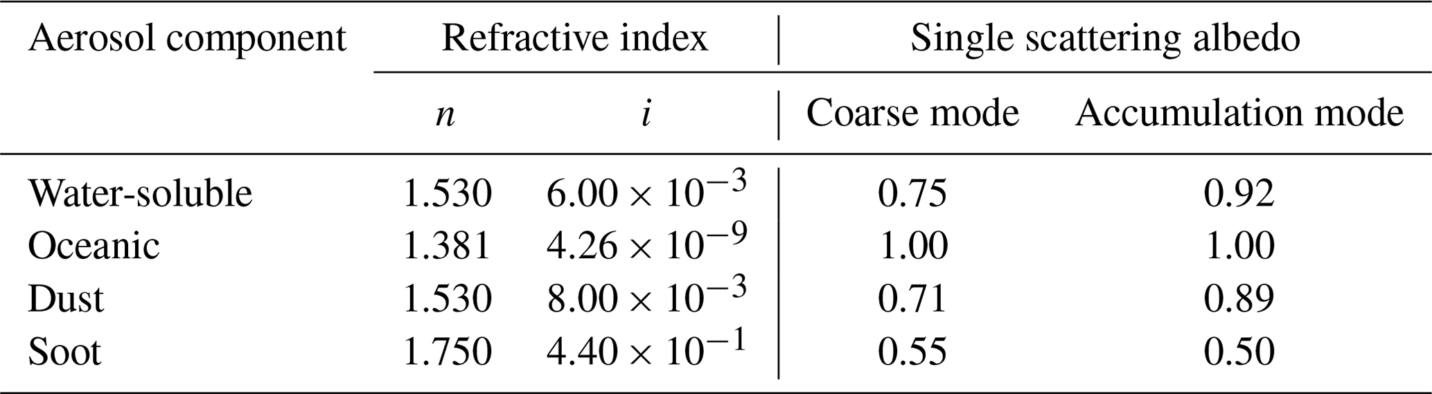
The aerosol properties used in model simulations, such as the single scattering albedo (SSA (λ)), the real part, and the imaginary part of the refractive index for the coarse and accumulation modes of the water-soluble, oceanic, dust, and soot aerosol components are given in Table 1 adopted from Istomina et al. (2011). Subsequently, a look-up table was calculated using the SCIATRAN radiative transfer model (Rozanov et al., 2014; Mei et al., 2023). This look-up table has been used for the determination of ${\mathit{\rho }}_{\mathrm{atm}}(\mathit{\lambda },{\mathit{\mu }}_{\mathrm{0}},\mathit{\mu },\mathit{\varphi },\mathit{\tau })$.

In addition to the usage of the NDSI and ASCIA, a combination of seven AATSR channels was used to distinguish the spectral response of a clear, snow-covered landscape from that of clouds, land, and sea using the visible (Eqs. 14, 15) and near-infrared (Eq. 13) nadir reflectances of the top of the atmosphere. The VIS and NIR criteria (Eqs. 13, 14, and 15) select scenes whose spectral behavior is similar to the snow spectrum (Istomina et al., 2009).

$$\begin{array}{}\text{(13)}& {\displaystyle \frac{{\mathit{\rho }}_{\mathrm{atm}}\left(\mathrm{0.87}\mathrm{\mu }\mathrm{m},{\mathit{\mu }}_{\mathrm{0}},\mathit{\mu },\mathit{\varphi }\right)-{\mathit{\rho }}_{\mathrm{atm}}\left(\mathrm{1.6}\mathrm{\mu }\mathrm{m},{\mathit{\mu }}_{\mathrm{0}},\mathit{\mu },\mathit{\varphi }\right)}{{\mathit{\rho }}_{\mathrm{atm}}\left(\mathrm{0.87}\mathrm{\mu }\mathrm{m},{\mathit{\mu }}_{\mathrm{0}},\mathit{\mu },\mathit{\varphi }\right)}}>\mathrm{80}\mathit{\%}\text{(14)}& {\displaystyle \frac{{\mathit{\rho }}_{\mathrm{TOA}}\left(\mathrm{0.87}\mathrm{\mu }\mathrm{m}\right)-{\mathit{\rho }}_{\mathrm{TOA}}\left(\mathrm{0.66}\mathrm{\mu }\mathrm{m}\right)}{{\mathit{\rho }}_{\mathrm{TOA}}\left(\mathrm{0.87}\mathrm{\mu }\mathrm{m}\right)}}<\mathrm{10}\mathit{\%}\text{(15)}& {\displaystyle }\left|{\displaystyle \frac{{\mathit{\rho }}_{\mathrm{TOA}}\left(\mathrm{0.66}\mathrm{\mu }\mathrm{m}\right)-{\mathit{\rho }}_{\mathrm{TOA}}\left(\mathrm{0.55}\mathrm{\mu }\mathrm{m}\right)}{{\mathit{\rho }}_{\mathrm{TOA}}\left(\mathrm{0.66}\mathrm{\mu }\mathrm{m}\right)}}\right|<\mathrm{10}\mathit{\%}\end{array}$$

R_TOA is the reflection at the top of the atmosphere.

Table 1 Single scattering albedo (SSA), real “n”, and imaginary “i” parts of the refractive index for coarse and accumulation modes of water-soluble, oceanic, dust, and soot aerosol components at 555 nm (Istomina et al., 2009).

3.2 Data quality flagging

Quality flagging of the AOD data product gives information about our assessment of the accuracy of the AOD determined using AEROSNOW. To compare the AOD of AERONET, measured at 500 nm, with that of AEROSNOW, measured at 555 nm, a conversion is required. The AOD at 500 nm is extrapolated to the AOD at 555 nm by using the Ångström exponent determined in the 500–870 nm region. We consider the AOD at 555 nm to be the total AOD of the atmosphere. This was validated by comparisons with the AERONET AOD. For these comparisons, the AEROSNOW observations were averaged within a 25 km radius of the AERONET station and within a ±30 min period of the AERONET measurement. Monthly averages of these AEROSNOW spatiotemporal collocated data were generated. Information about the derived collocated daily values is shown in Appendix A (Fig. A1).

In postprocessing AEROSNOW results, we selected optimal conditions, i.e., by using a cutoff value for the solar zenith angle (≥75^∘) and filtering out those scenes or pixels that had an NDSI value of ≤0.97. In this work, we adopted the recommendations in Istomina (2011, Sect. 3.3.5) for an SZA of 75^∘ based on sensitivity analysis using the SCIATRAN radiative transfer model (see also Mei et al., 2023).

In this study, the NDSI was used in rigorous postprocessing of the datasets to filter out the mixed and snow-free regions. For the stations considered in this study, we found bimodal distributions of AOD, with the frequency at higher AOD values influenced by clouds and problematic surfaces. We filtered out 40 % over problematic surfaces and residual clouds and 100 % over central Greenland using rigid postprocessing by applying the NDSI filter. The AEROSNOW retrieval is based on Eqs. (4) to (10) and uses the ratio of the simulated nadir BRDF values for the nadir and forward views of the dual-viewing AATSR instrument. With this strategy, we mitigate the absolute errors in the BRDF but rather rely on the shape of the BRDF as seen from both directions. For our study, a narrow interval of the NDSI was required to limit the BRDF-induced error in retrieving the AOD, which is less than 30 % using the Istomina (2011) approach (Sect. 3.3.3). We additionally introduced the QF approach in our postprocessing scheme by adopting independent additional support from MODIS Terra and Aqua cloud fractions (Ackerman et al., 2008) apart from the ASCIA cloud detection algorithm, where we weighted the snow cover fraction even higher than the cloud fraction.

According to Liu et al. (2022), the discrepancies caused by different sensors and different algorithms for the MODIS Terra and Aqua CF products over the Arctic are ±2 % and ±5 % with respect to the International Arctic Systems for Observing the Atmosphere (IASOA). The exact locations of the IASOA observatories are shown in Fig. 1 of Uttal et al. (2016).

To ensure quality, we also noted that melt ponds and thin clouds not captured by rigid filtering deteriorate the retrieval quality of AEROSNOW. Recently, Xian et al. (2022) introduced a postprocessing scheme to remove erroneous AOD outliers. Instead of applying the rather qualitative quality-flagging approach as proposed by the former, we applied a more quantitative one. We thoroughly examined the ratio of AEROSNOW AOD to AERONET AOD greater than a factor of 1.6 by calculating a QF parameter $[\text{QF}=(\mathrm{0.8}\times \left(\text{snow cover fraction}\right)+\mathrm{0.2}\times (\mathrm{1}-\text{cloud fraction})]$ which penalizes the low levels of snow cover and (to a lesser extent) residual cloud fraction by using MODIS Terra and Aqua data products from NASA Worldview (https://worldview.earthdata.nasa.gov/, last access: 3 February 2022), respectively. When using the AEROSNOW data beyond the AERONET stations, we applied this scheme to all data points of AEROSNOW. Empirical tests showed that an appropriate snow cover fraction is weighted higher than an appropriate clear-sky fraction (1− cloud fraction). This is expressed by the individual weighting factors for snow cover fraction (0.8) and clear-sky fraction (0.2). We found that a QF threshold value of 0.6 represents a compromise between data yield and data quality. Thus, in the final step, AOD values with a QF value of 0.6 or less were removed.

4 Result: assessment of AEROSNOW AOD

4.1 Qualitative analysis of AEROSNOW

Before we turn to quantitative validation of the AEROSNOW results, here we briefly discuss the spatiotemporal distribution of the AEROSNOW data in qualitative terms. The spatiotemporal frequency of observations over the Arctic from both ground and satellites is greater in summer (JJA) than in spring (MAM). Figure 4a shows the monthly averaged AOD over snow and Arctic ice for the period 2003–2011, with significant differences in the spatial distribution of AOD. Figure 4b shows the number of pixels used to average AOD per grid cell during 2003–2011 for March through October.

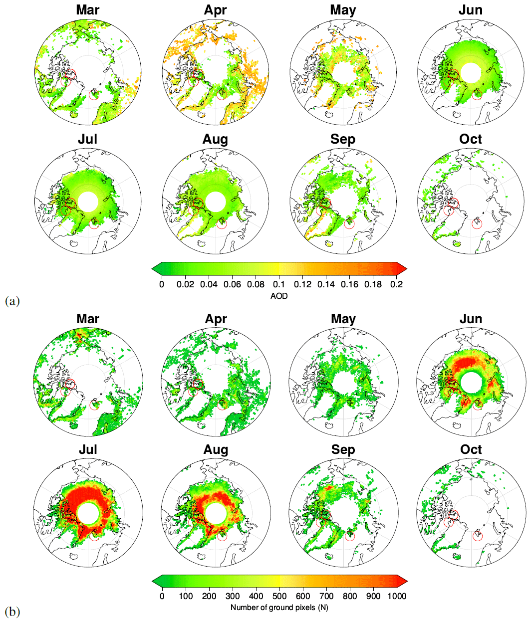
Figure 4 (a) Pan-Arctic seasonal view of AEROSNOW-retrieved AOD over snow and ice averaged from the years 2003 to 2011 for the months March to October, i.e., large parts of the period of insolation. Red circles indicate the locations of AERONET stations. (b) Pan-Arctic seasonal view of the AEROSNOW-retrieved number of ground pixels (N) constituting the monthly average AOD over snow and ice averaged from the years 2003 to 2011 for the months March to October, i.e., large parts of the period of insolation. Red circles indicate the locations of AERONET stations for guidance. The size of the red circles is not identical to the spatial collocation radius of 25 km, which we have used in the validation.

In this study, satellite retrievals are performed only when snow and ice are present (NDSI threshold values; see Sect. 2). The NDSI was used to constrain the BRDF in terms of snow grain size and impurity (when snow accumulation is fresh), and clouds are absent. Accordingly, the best coverage is obtained over persistently homogeneous areas covered with (fresh) snow and ice. Greenland is an exception to the AOD retrieval. Possible reasons for this could be that the BRDF does not fit well because it does not adequately represent the snow grains and impurities of the Greenland glaciers, the snow-covered ice sheet, and the elevated topography. Further, the clouds over Greenland are typically optically thin and low-hanging (Bennartz et al., 2013) and are likely not all captured by the ASCIA cloud detection algorithm. Smoother patterns are observed in Fig. 4 over the Arctic sea ice compared to snow-covered land.

4.2 Statistical evaluation of AODs from AERONET and AEROSNOW

In the next step, satellite-retrieved and ground-based observations are compared. Figure 5 shows the validation between AEROSNOW-retrieved AOD over the PEARL, OPAL, Hornsund, and Thule and AERONET AOD during this study period. Figure A1 in Appendix A depicts daily collocated values and statistics.

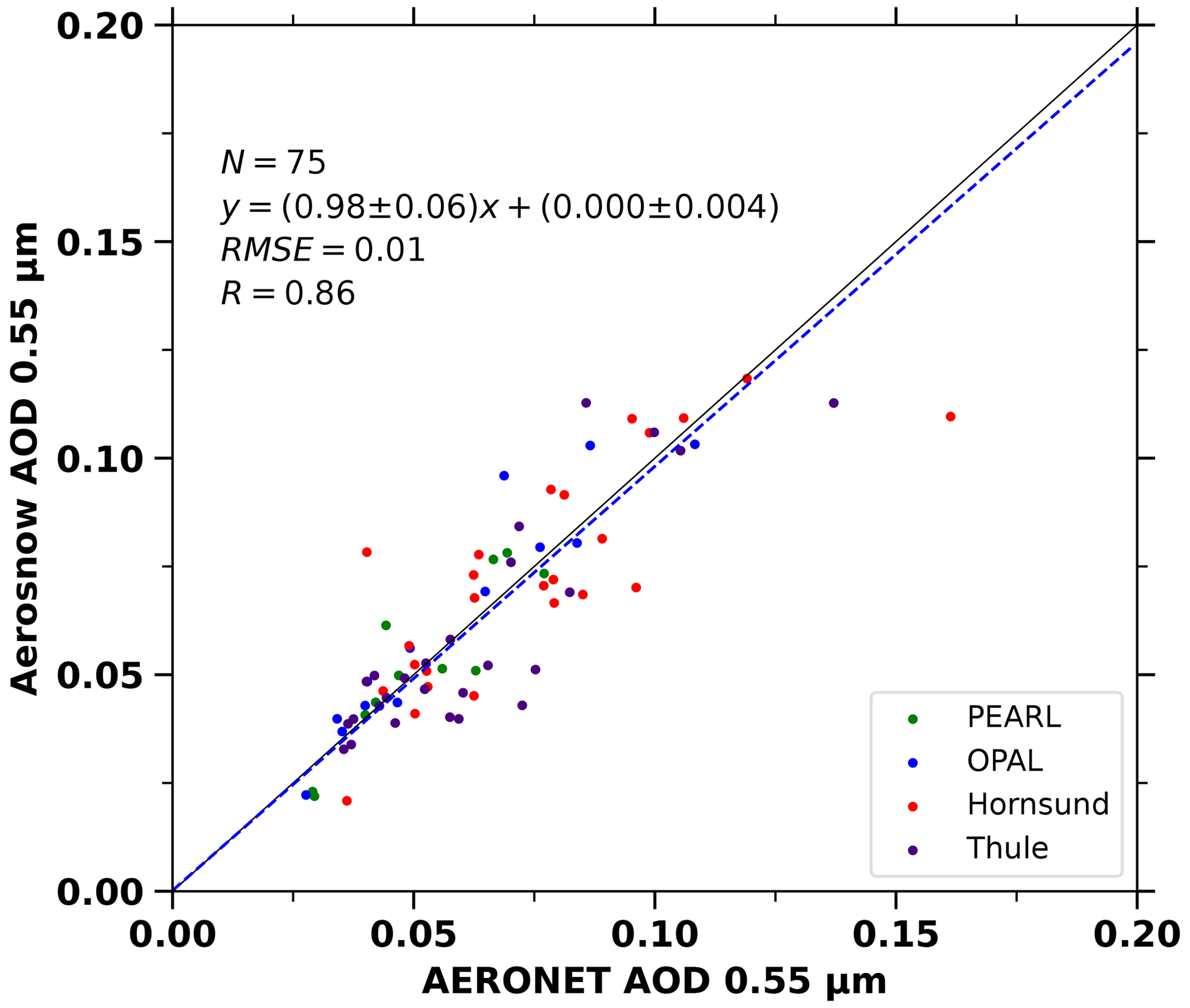
Figure 5 Validation of monthly mean AEROSNOW-retrieved AOD collocated with monthly mean AERONET observation AOD obtained over the PEARL, OPAL, Hornsund, and Thule stations. The linear regression line is shown as the blue dashed line.

Much of the data analysis in this paper involves fitting a straight line to the AODs observed by both AERONET and AEROSNOW. Because the AOD observations by these two platforms are both subject to measurement errors (Sinyuk et al., 2012; Mei et al., 2013), we have used a fitting procedure known as the reduced major axis (RMA) method, as described by Hirsch and Gilroy (1984) and Ayers (2001).

RMA regression takes into account the uncertainties or errors of the two variables, while ordinary least squares (OLS) regression takes into account the uncertainties of one variable. Here, the best linear fit between the two variables is sought, which must be the same in X or Y regardless of the variable, i.e., aiming for a symmetric relationship. For this, different methods are possible, e.g., by minimizing the perpendicular distance or the triangle, and we choose the RMA, i.e., by minimizing the triangle. RMA has been used by other researchers in the analysis of air quality and atmospheric chemistry data: see, e.g., Keene et al. (1986), Arimoto et al. (1995), Freijer and Bloemen (2000), Ayers (2001), and Wang et al. (2004).

By combining these four stations, the coefficient of correlation (R) is on average 0.86 and the RMSE is 0.01. Validating each station separately, the R value increases to 0.90, 0.94, 0.81, and 0.87 over PEARL, OPAL, Hornsund, and Thule, respectively (Fig. 6). We consider R values of about 0.8 to be sufficient by keeping in mind that these retrievals are very challenging over the Arctic.

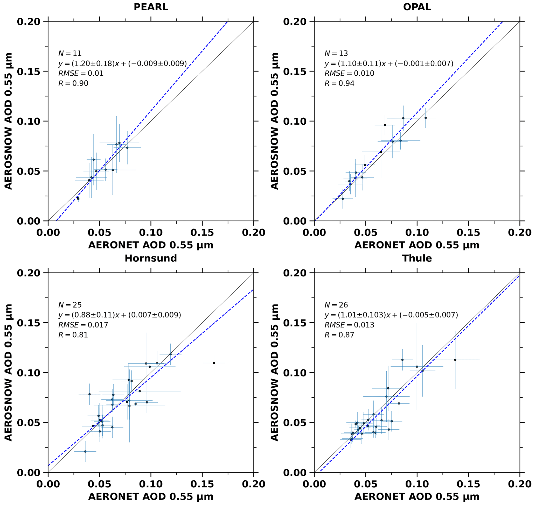
Figure 6 Validation of monthly mean AEROSNOW-retrieved AOD collocated with monthly mean AERONET observation AOD obtained over the PEARL, OPAL, Hornsund, and Thule stations. The linear regression lines are shown as blue dashed lines.

4.3 Comparison of AODs from AERONET and AEROSNOW

In the next step, we analyze the collocated temporal evolution of the AEROSNOW results and compare them with AERONET station data. The time series of retrieved AEROSNOW AOD is shown together with AERONET data in Fig. 7. In general, the time series for AERONET is well reproduced by AEROSNOW.

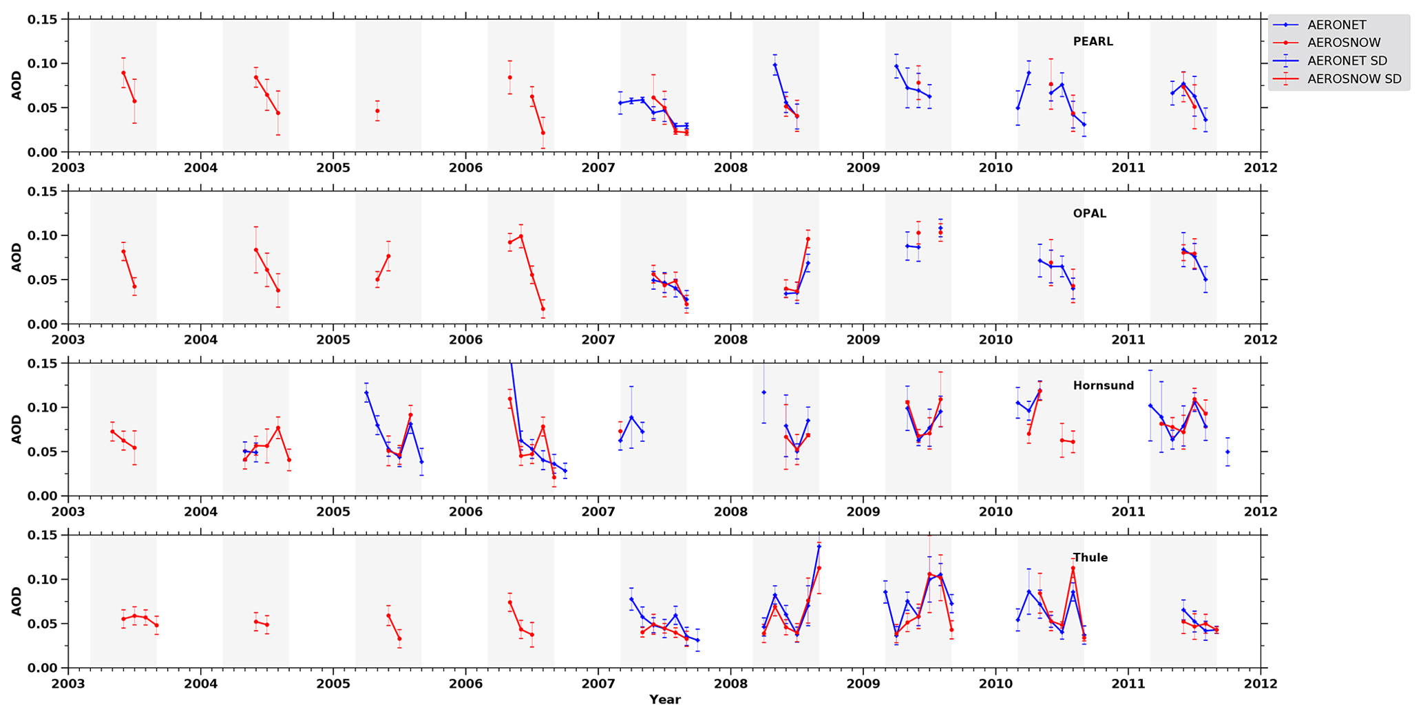
Figure 7 Monthly mean time series of AERONET and AEROSNOW AOD at the PEARL, OPAL, Hornsund, and Thule stations. The MAM and JJA periods are highlighted with light grey shading.

In general, and as expected, we observe that PEARL, OPAL, and Thule (extended Canadian archipelago, henceforth called CA stations) exhibit similar temporal behavior. The PEARL and OPAL AERONET sites are located around 11.5 km apart. OPAL is closer to the coast than the PEARL station; they are located at altitudes of 5.0 and 615.0 m, respectively. Hornsund is clearly different in this context.

The CA stations show low average AOD values. This is associated with Arctic background scenarios. The seasonal variability over all these three stations is presented in Fig. 8, which shows that both the AEROSNOW and AERONET results exhibit higher AOD during spring (MAM) and minimum AOD during summer (JJA). A partially high estimation of AEROSNOW is observed over all the selected sites in August, which may be due to uncertainties in surface parameterization and aerosol types in this region.

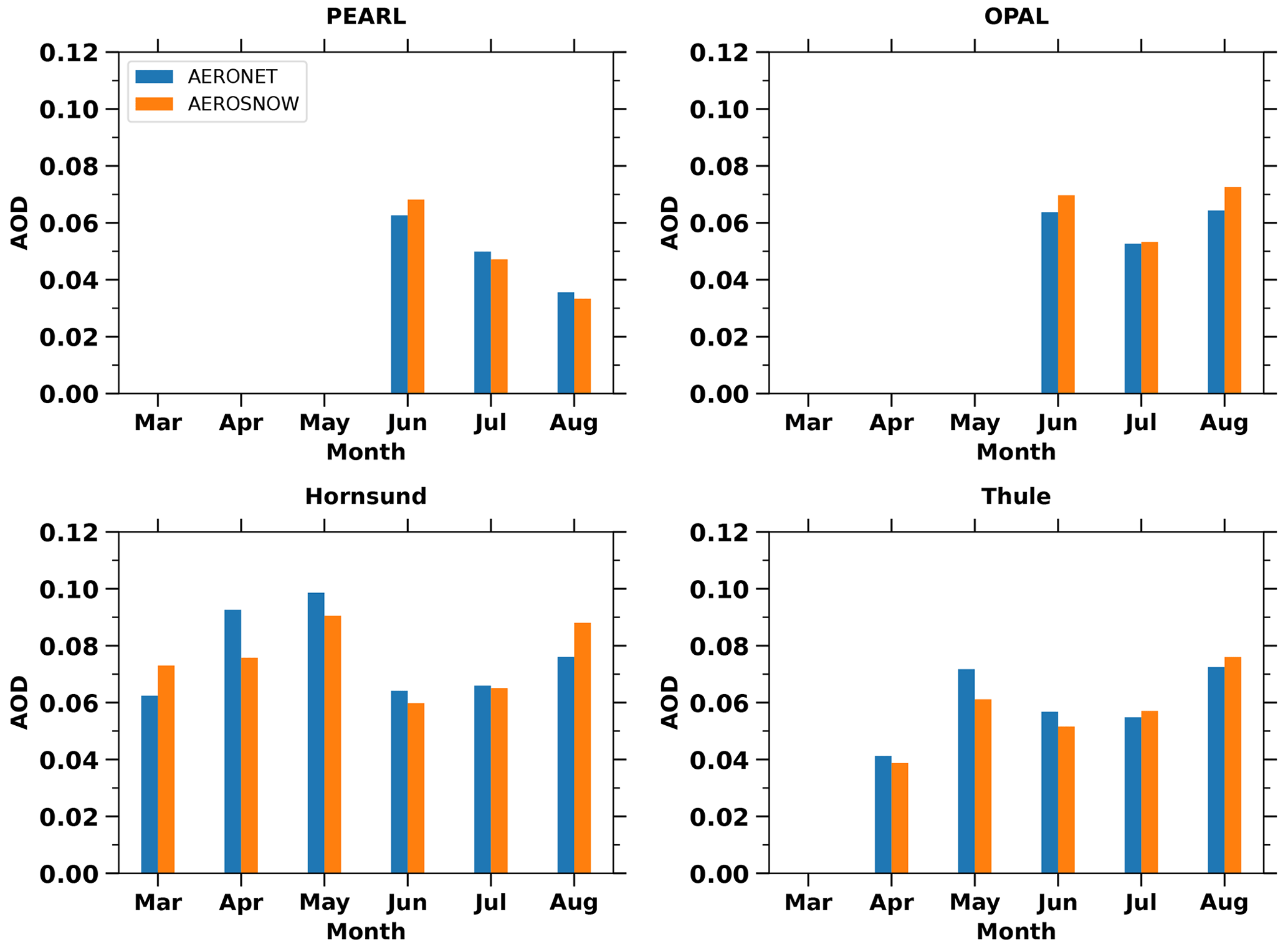
Figure 8 Seasonal AOD variation over PEARL, OPAL, Hornsund, and Thule with AEROSNOW and AERONET values averaged from 2003 to 2011. Blue and orange bar plots show statistics for AERONET and AEROSNOW, respectively.

On average, AEROSNOW appears to capture some haze events during spring and thereby has higher average values than in the summer season.

4.4 Springtime and summertime AOD over the Arctic sea ice

Similar to the analysis shown in Fig. 7, where we examined the time series of total AOD from AEROSNOW over AERONET stations, we now discuss qualitatively how AOD values change over time across the entire region of Arctic sea ice.

The AEROSNOW AOD results over pan-Arctic sea ice shown in Figs. 9 and 10 exhibit maximum values in spring 2009 and minimum values in spring 2006. However, comparing the seasonally averaged climatology from 2003 to 2011, the AEROSNOW results indicate higher AOD values in spring and smaller values in summer as shown in Figs. 9 and 11, which was expected due to the Arctic haze events (Willis et al., 2018).

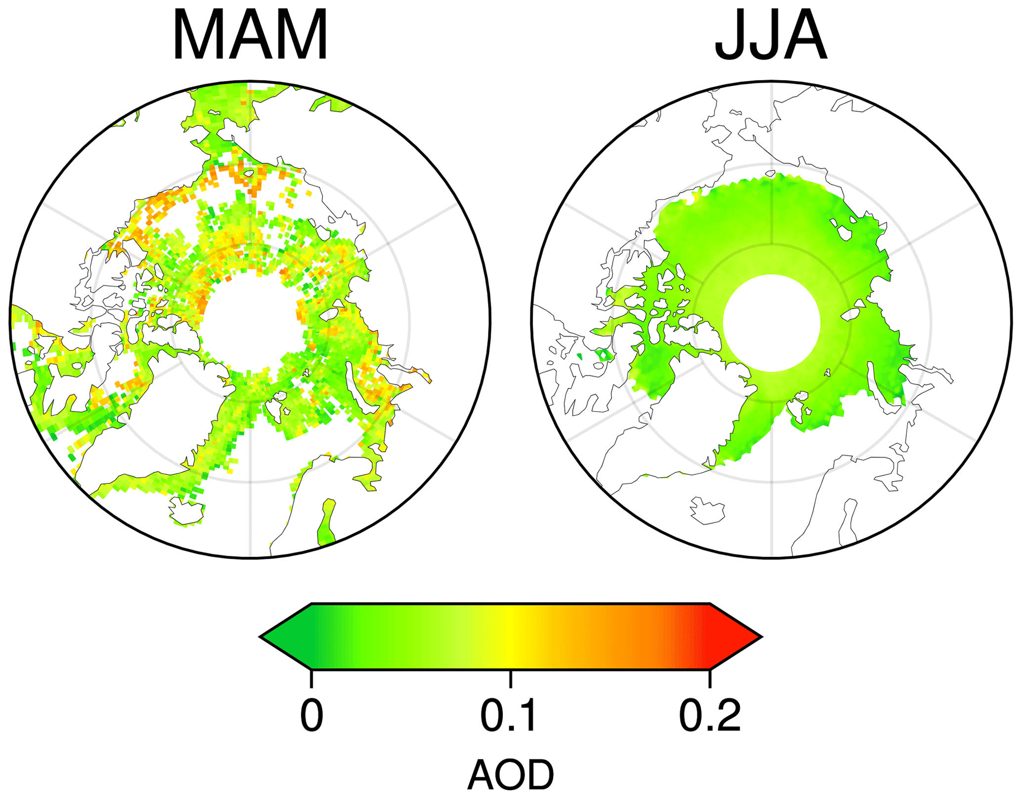
Figure 9 Mean climatological MAM and JJA AEROSNOW-derived AOD over Arctic sea ice averaged from the years 2003 to 2011. The white area shows a lack of data apart from the masked land area.

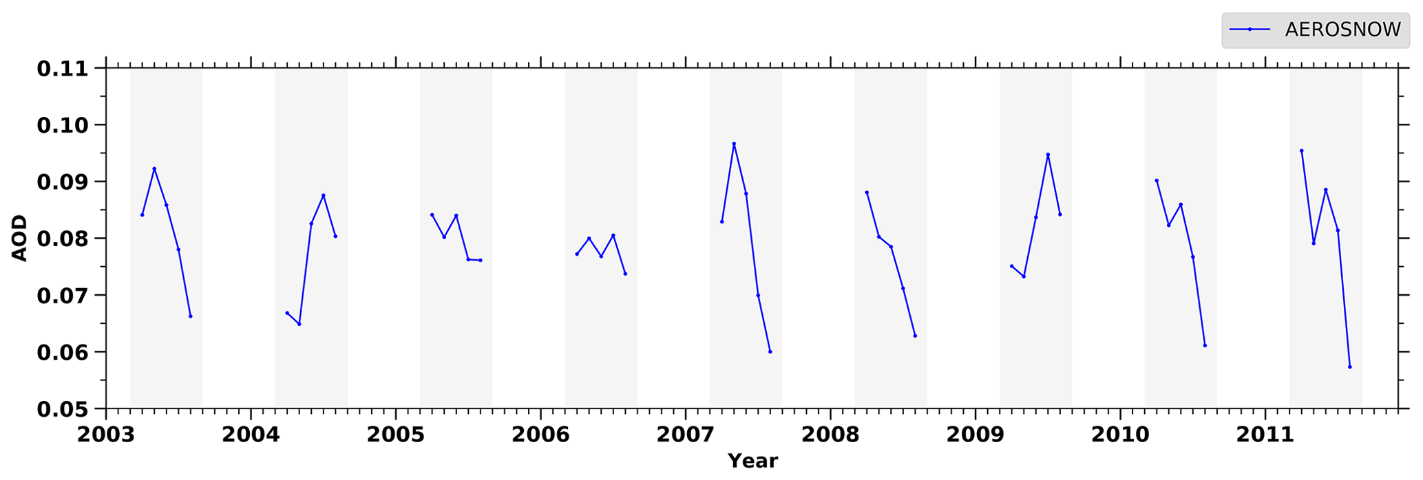
Figure 10 Monthly mean time series of AEROSNOW AOD over the Arctic sea ice region. The MAM and JJA periods are highlighted with light grey shading.

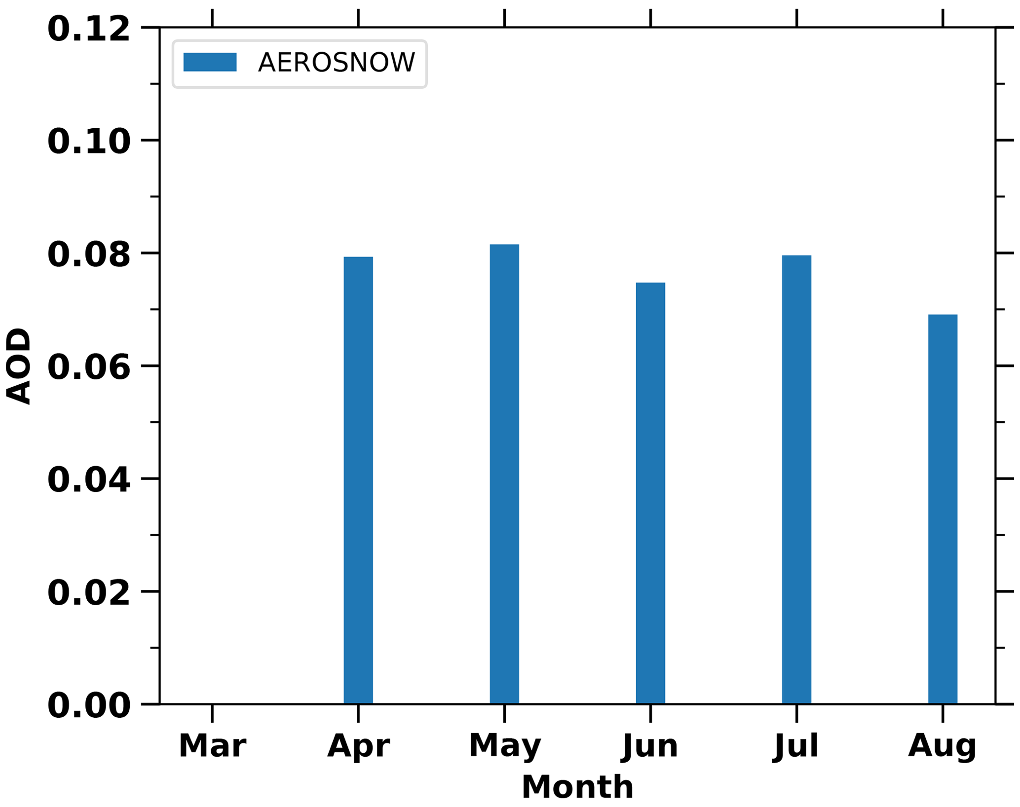
Figure 11 Seasonal AOD variation in Arctic sea ice region values averaged from 2003 to 2011. Blue bars denote the observed monthly mean AODs of AEROSNOW.

On the other hand, the AEROSNOW retrievals of AOD may be affected by cloud contamination because high levels of cloud cover are observed over the Arctic in summer, with average values around 0.8 (Kato et al., 2006). Although we adopted reasonable cloud masking for the AOD retrievals, we cannot exclude entirely the possibility that residual cloud contamination might prevail (Jafariserajehlou et al., 2019). Additionally, AEROSNOW captures the higher values of AOD over northern Alaska and Siberia during summer, a region which is often influenced by boreal forest fires during this period (Xian et al., 2022) (Fig. 9). During spring higher values of AOD (0.1–0.12) are observed near Europe and the Asian continent and smaller values (0.07–0.08) towards the CA.

Spring values are mostly dominated by long-range transport of anthropogenic aerosols from the lower latitudes of Europe, America, and Asia (Willis et al., 2018). The AEROSNOW estimates of AOD over central Arctic sea ice are reasonable and thus a valuable source for filling the aerosol data deficit over the perennial sea ice region in the high Arctic.

5 Conclusions

This is the first time that AOD has been retrieved using satellite data over the entire Arctic snow and ice surface over a 9-year period and validated with ground-based AERONET measurement. A satellite-based retrieval of AOD over Arctic snow and ice was conducted, which has been shown to fill the gap in data availability from standard aerosol products, e.g., MODIS. The AEROSNOW algorithm uses the dual-viewing capability of the AATSR instrument to minimize retrieval uncertainties (Istomina et al., 2009, 2011; Mei et al., 2013). It showed good agreement with ground-based AERONET observations, with a correlation coefficient of R=0.86 and a low systematic bias.

The high anthropogenic aerosol loading (Arctic haze events) due to long-range transport (Willis et al., 2018) over Arctic snow and ice is captured by the AOD determined by AEROSNOW. Further, the monthly mean spatial maps shown in Fig. 4 confirmed that the haze events are captured well. The time series and seasonality of the AEROSNOW AOD agree well with AERONET observations. Good agreement between AEROSNOW and AERONET AODs is achieved over the PEARL, OPAL, Hornsund, and Thule stations. The AEROSNOW-retrieved AOD shows maximum values during spring (MAM) and minimum values during summer (JJA), which is also in accordance with AERONET measurements. Further improvement of the AOD retrieval could be possible in terms of cloud masking, surface reflectivity properties, and the adoption of more appropriate aerosol types to be considered.

The promising AOD results obtained with AEROSNOW indicate that these can be used to evaluate and improve aerosol predictions for various chemical transport models (Willis et al., 2018), especially over the Arctic sea ice in spring and summer for the important period 2003–2011, which is within the period of Arctic amplification.

Appendix A: Additional figures

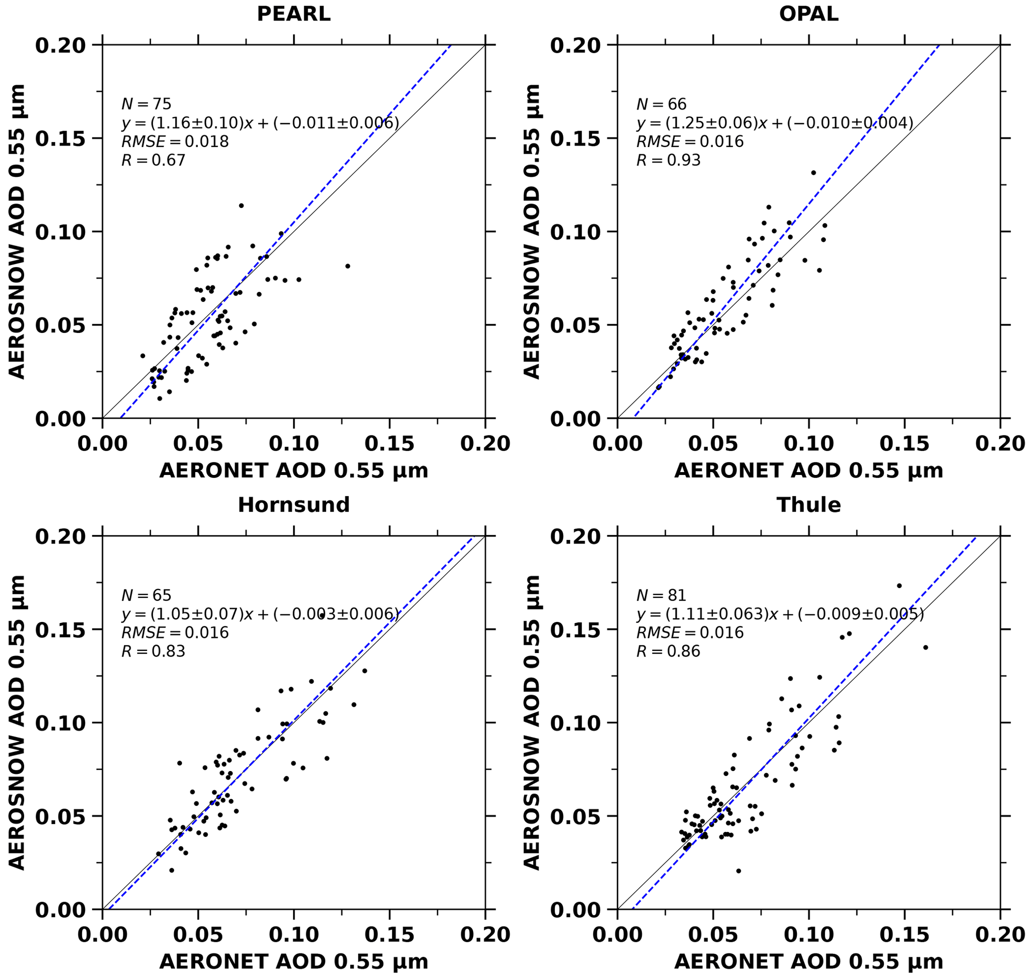
Figure A1 Validation of daily AEROSNOW-retrieved AOD collocated with daily AERONET observation AOD obtained over the PEARL, OPAL, Hornsund, and Thule stations. The linear regression lines are shown as blue dashed lines.