the Creative Commons Attribution 4.0 License.
the Creative Commons Attribution 4.0 License.
 | 13 Jun 2024
Stability requirements of satellites to detect long-term stratospheric ozone trends based upon Monte Carlo simulations
For new satellite instruments, specifications of the stability required for climate variables are provided in order to be useful for certain applications – for instance, deriving long-term trends. The stability is usually stated in units of percent per decade (% per decade) and is often associated with or termed instrument drift. A stability requirement of 3 % per decade or better has been recently stated for tropospheric and stratospheric ozone. However, the way this number is derived is not clear. In this study, we use Monte Carlo simulations to investigate how a stability requirement translates into uncertainties in long-term trends depending on the lifetime of individual observing systems, which are merged into time series, and the period of available observations. Depending on the need to observe a certain trend over a given period, e.g., typically +1 % per decade for total ozone and +2 % per decade for stratospheric ozone over 30 years, stability for observation systems can be properly specified and justified in order to achieve statistical significance in the observed long-term trend. Assuming a typical mean lifetime of 7 years for an individual observing system and a stability of 3 % per decade results in a 2 % per decade trend uncertainty over a period of 30 years, which is barely sufficient for stratospheric ozone but too high for total ozone. Having two or three observing systems simultaneously reduces the uncertainty by 30 % and 42 %, respectively. Such redundancies may be more efficient than developing satellite instruments with higher long-term stability to reduce long-term trend uncertainties. The method presented here is applicable to any variable of interest for which long-term changes are to be detected.
- Article
(4770 KB) - Full-text XML
- BibTeX
- EndNote


Of the ozone in the overhead (total) column, 90 % resides in the stratosphere and protects the Earth system from harmful UV radiation (Zerefos et al., 2023). The phaseout of ozone-depleting substances (ODS), according to the Montreal Protocol and its amendments, leads to recovery of stratospheric ozone in some regions of the atmosphere after the late 1990s (Hassler et al., 2022). Statistically significant trends are observed in the upper stratosphere, with an increase of up to about +2 % per decade (Godin-Beekmann et al., 2022). In the extratropics, total column ozone has increased by a rate of up to about +1 % per decade (Coldewey-Egbers et al., 2022; Weber et al., 2022). The reported statistical trend uncertainty at the 2σ level for ozone profiles is typically of the same order as the trend itself at about 1 %–2 % per decade, and similarly for total column ozone at about 0.5 %–1 % per decade (SPARC/IO3C/GAW, 2019; Godin-Beekmann et al., 2022; Weber et al., 2018, 2022).
Uncertainties in ozone trends reported recently (e.g., Hassler et al., 2022; Godin-Beekmann et al., 2022; Weber et al., 2022) are determined from the statistics of trend regression alone. Bourassa et al. (2014) reported added uncertainties due to drifts of the OSIRIS satellite to the statistical uncertainty, here at 3 % per decade, which reduced the atmospheric region (altitude and latitude) of the atmosphere showing significant positive trends. A direct comparison between various merged ozone profiles shows that the drifts in the difference between zonal mean single-instrument datasets are on the order of 3 % per decade (2σ) but not always statistically significant (Rahpoe et al., 2015; Hubert et al., 2016). Similarly, the spread in the recent total ozone trends from the available merged datasets is on the order of ±0.5 % per decade (2σ). The apparent drifts are not only due to changes in the instrument performance, but can also be dependent on how the individual datasets are merged into the long-term dataset (Frith et al., 2017; Weber et al., 2022). Since multiple time series are available, the statistical trend uncertainty can be further reduced by averaging trends or calculating trends from the median or mean of datasets (e.g., Steinbrecht et al., 2017; SPARC/IO3C/GAW, 2019; Godin-Beekmann et al., 2022; Weber et al., 2022).
Ozone is expected to recover from the decrease in ozone-depleting substances, but long-term changes also depend on the evolution of greenhouse gases (GHGs) as well as on the feedback mechanism between ozone and climate (Hassler et al., 2022). The Vienna Convention for the Protection of the Ozone Layer (United Nations, 1985), which set, among others, the framework for the Montreal Protocol signed in 1987, also stated the need for continuing the observation of ozone, related species, and climate gases. For long-term observations of ozone and other trace species, specific requirements of accuracy and stability for observing systems were defined and updated over the years (e.g., World Meteorological Organisation, 2001, 2004, 2011; CCI, 2021; CMUG, 2022; World Meteorological Organisation, 2022). For trend detection, a stability requirement of 3 % per decade was initially stated for stratospheric ozone and 1 % per decade for total ozone (World Meteorological Organisation, 2001). Main application areas defined were trends and operational meteorology for stratospheric ozone (World Meteorological Organisation, 2001). The 3 % per decade value is also currently defined as the threshold value for stratospheric profiles and total column of ozone, meaning that a satellite instrument will only be useful if this threshold is not exceeded (CCI, 2021; World Meteorological Organisation, 2022; CMUG, 2022). In addition to the threshold value, a breakthrough (2 % per decade) and target value (1 % per decade) are provided (World Meteorological Organisation, 2022). No specification in these documents is given regarding if the stability requirement is stated as one (1σ) or 2 standard deviations (2σ). With regard to the observed long-term ozone trends, these values only make sense if they are defined as 2σ (2 standard deviations).
It is not clear how these specifications are derived, but they are very likely derived from the observed statistical ozone trend uncertainties and the expectation that the requirements should be close but lower than these uncertainties. The question we raise here in the paper is how such a requirement can be justified by the need to achieve a certain trend uncertainty over a given period of time. From the ozone recovery perspective, the time range since ODS peaked in the stratosphere is close to 30 years. A similar but different question was addressed by Weatherhead et al. (1998). Based upon the noise of data and serial correlation, they determined, on statistical grounds, how many years we need to observe a significant trend, which occurs when twice the trend uncertainty is lower than the trend magnitude (2σ significance).
We use Monte Carlo simulations to investigate how a stability requirement translates into uncertainties in long-term trends depending on the lifetime of individual satellite instruments, which are merged into long-term time series, and the overall period of available observations. In Sect. 2, the scheme of the Monte Carlo simulation is described. Results are presented in Sect. 3 and discussed in Sect. 4. We close with concluding remarks in Sect. 5.
The scheme of Monte Carlo simulations of time series and derived trend uncertainties due to a given stability requirement are shown in Fig. 1 (e.g., Guimaräes Couto et al., 2013). We assume that a simulated time series is zero without any drift and bias after the subtraction of the start value. Each individual observing system with a given lifetime (segment) of which we compose a long-term merged dataset (time series) has varying drifts in % per decade, which follow a Gaussian distribution with a given 1σ stability requirement (e.g., 1.5 % per decade, as shown in Fig. 1a). The variability seen in the sample of 1 million long-term time series (Fig. 1b) is therefore solely due to the instrument drifts following the stability distribution. As an example, four single time series over 30 years are shown in red. Each segment is 7 years long, corresponding to a constant lifetime. For simplicity, an overlap period is not considered here (Weatherhead et al., 2017).
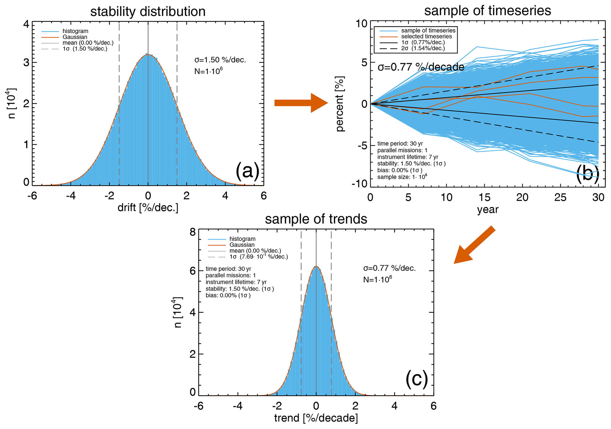
Figure 1Monte Carlo simulation of 30-year trend uncertainties, assuming a stability requirement of 3 % per decade (2σ) for individual observing systems, with a lifetime of 7 years. (a) Gaussian instrumental drift distribution, assuming a stability requirement of 3 % per decade (2σ). (b) 10 000 time series (blue lines) from 1 million samples of simulated time series, composed of 7-year individual segments (single instrument observations). Red lines show four examples of time series from the sample. (c) Distribution of linear trends derived from all time series.
For each of the time series, a simple linear trend was fit and the distribution of trends, and its width representing the trend uncertainty given by the standard deviation of the distribution is shown in Fig. 1c. Here, the trends are calculated for a 30-year period. A stability requirement of 1.5 % per decade (1σ) and a lifetime of 7 years for each observing system result in a trend uncertainty of 0.77 % per decade after 30 years (close to half the value of the stability requirement). With a required limit of stability of 3 % per decade (2σ) for ozone, trends lower than about 1.5 % per decade (2σ) are not detectable after 30 years (simply doubling the numbers given in the previous sentence).
Some additional modifications in the simulation were introduced. In a merged dataset, the individual observing systems have varying lifetimes. An expected lifetime of 7 years is typical of current satellite systems, e.g., TROPOMI (Veefkind et al., 2012). Several satellite instruments measured for a decade or more (e.g., SAGE II for 21 years; OSIRIS for more than 20 years; OMI for 19 years; GOME-2A for 12 years; and SCIAMACHY, MIPAS, and GOMOS for 10 years). In a different setup, we therefore vary the lifetimes of individual segments following a Poisson distribution with a mean of 7 years (Fig. 2). Later, we also show results for instruments with a longer mean lifetime of 12 years, When merging datasets, usually segments of a single observation system with some extended records are used. In our case, we set a lower limit of 5 years to be included in the time series.
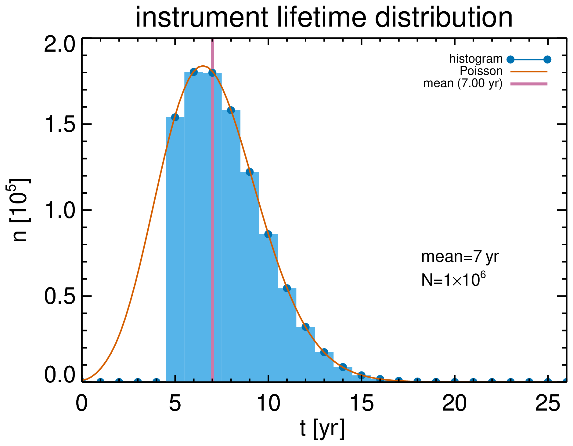
Figure 2Distribution of lifetimes for single observing systems based upon a Poisson distribution with a mean of 7 years. Segments with lifetimes of less than 5 years are not allowed in the time series and the distribution is set to zero below 5 years.
Additional uncertainties come from biases between individuals segments. Biases can be corrected when sufficient overlap exists between observing systems, as discussed in detail in Weatherhead et al. (2017). In our simulations, we do not consider any overlap periods, but we allow for a Gaussian distributed bias from one segment to the other. Figure 3 shows the samples of time series assuming 0 %, 1 %, and 2 % bias (1σ), respectively. In both simulations, varying lifetimes with a mean of 7 years and Poisson distribution (Fig. 2) were assumed.
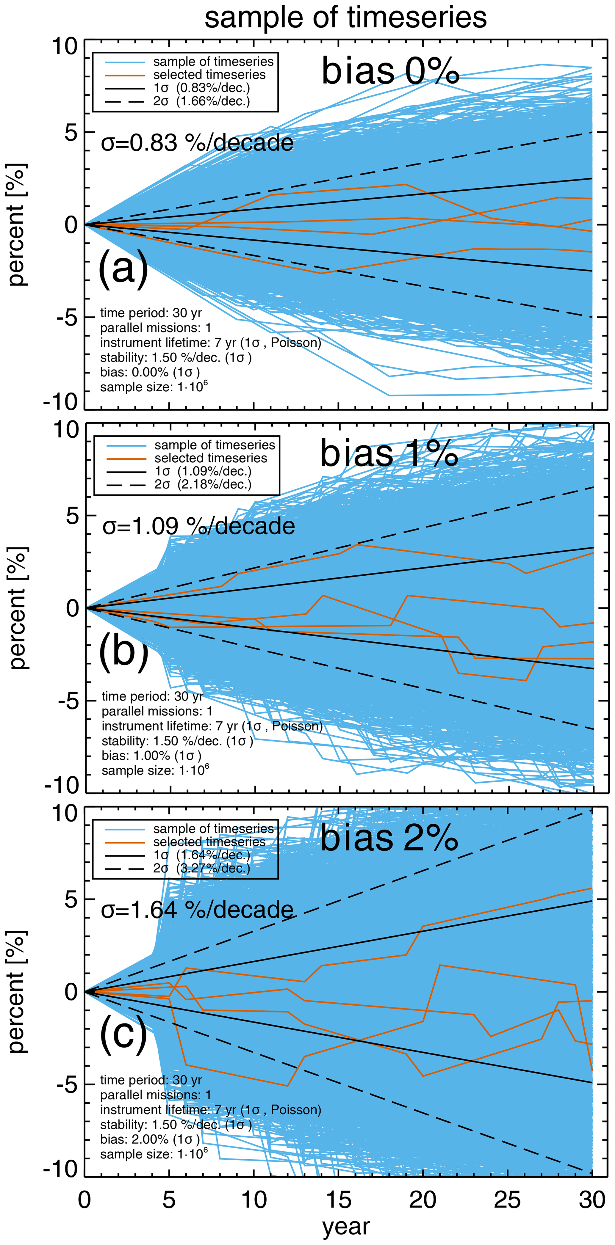
Figure 3Samples of 30-year time series composed of segments with varying lifetimes following a Poisson distribution with a mean and standard deviation of 7 years. 10 000 time series (blue lines) from 1 million samples of simulated time series, composed of 7-year individual segments (single instrument observations), are shown in each panel. Red lines show four examples of time series from the sample. (a) No bias between segments. (b, c) Biases drawn from a Gaussian distribution, with σ=1 % and 2 %, respectively.
With a stability requirement of 1.5 % per decade, the trend uncertainty after 30 years slightly increases from 0.77 % to 0.83 % per decade using varying lifetimes instead of a constant lifetime of 7 years (Figs. 2b and 3a). A larger change in uncertainties is seen by adding a 1 % bias between segments, resulting in an increase to 1.1 % per decade. This means that, for ozone observed with a 3 % per decade stability and a typical bias of 1 % between them, the trend uncertainty is 2.2 % per decade over 30 years.
The dependence of the trend uncertainty as a function of observation years, assuming a stability of 1.5 % per decade, is shown in Fig. 4. The different colors in the plot represent lifetimes for the individual observing systems, which vary from 5 to 20 years. For a given stability requirement and period of the time series, the trend uncertainties increase with lifetime. This is, at first sight, somewhat unexpected, as we normally desire to have observing or satellite missions operate as long as possible. A continuous drift over a longer time period causes larger deviations of the time series from the truth and increases trend uncertainties. It is also evident that the reduction in trend uncertainties with time slows considerably after 2 decades.
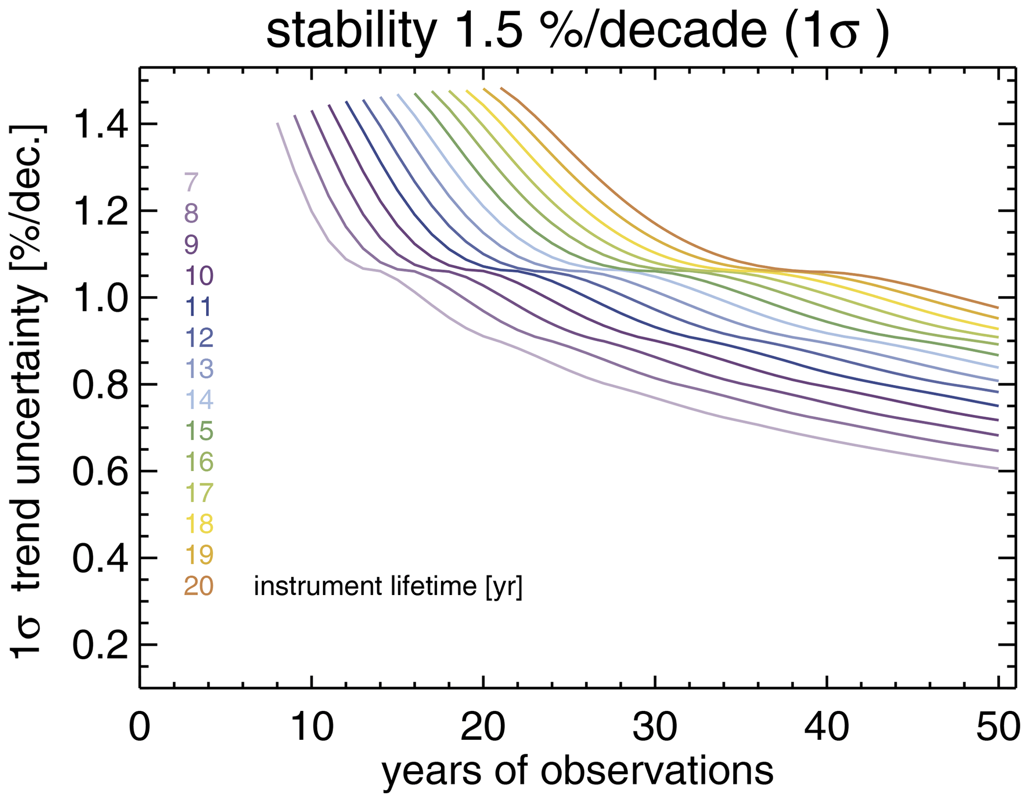
Figure 4Trend uncertainties as a function of the observation period, assuming a stability requirement of 1.5 % per decade for individual segments, with a constant lifetime. Different colors show results for lifetimes varying from 5 to 20 years.
So far, we have considered the case of one single mission contributing to the time series. If we have several parallel missions with identical geographical coverage for long-term monitoring, the trend uncertainties can be strongly reduced. To investigate this effect, mean time series were constructed by averaging n randomly generated time series, with n being interpreted as the number of parallel missions. The result is shown in Fig. 5. Trend uncertainties are reduced by a factor of from the single mission case. With two and three missions running in parallel over the entire period, the trend uncertainty is reduced by nearly 30 % and 42 %, respectively. Redundancy in satellites is therefore more effective in reducing trend uncertainties than improving the stability of a satellite instrument. This is an important consideration in a long-term monitoring program (Harris et al., 2015).
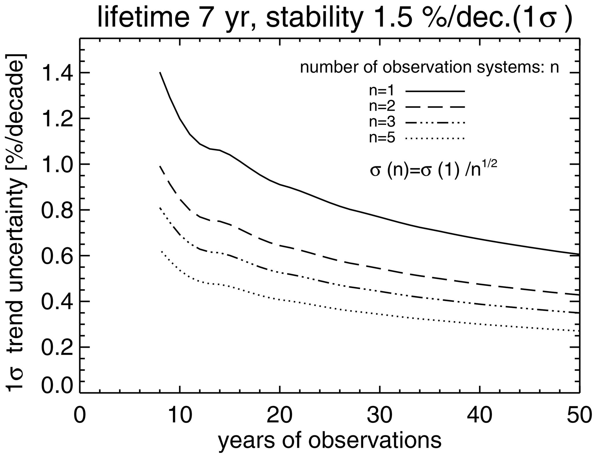
Figure 5Trend uncertainties as a function of the observation period and number of parallel satellites (n=1, 2, 3, and 5), assuming a constant lifetime of 7 years and a stability of 1.5 % per decade (1σ) for each satellite.
Figure 6 displays the impact of biases between segments on trend uncertainty as a function of the time series length. Here, we show in panels (a) to (c) the results for various stability requirements of 0.5 %, 1.0 %, and 1.5 % per decade (all 1σ), which correspond to the GCOS-22 requirements for target, breakthrough, and threshold, assuming they are given as 2σ values and results are shown for variable lifetimes with a mean of 7 (solid line) and 12 years (dashed line). If there are no biases (black curves in all panels), then the trend uncertainty decreases faster with time for lower lifetimes, as already demonstrated in Fig. 4. If the mean bias gets larger, this reverses and trend uncertainty decreases faster for time series with segments that have longer lifetimes. With a bias between consecutive satellite instruments, the trend uncertainty initially increases with time and starts decreasing after a couple of years, while the trend uncertainties in bias-free time series immediately decrease with additional years of data. Too large a bias causes the trend uncertainty to always be larger than the stability requirement (red and blue curves in Fig. 6a). One of the requirements for long-term monitoring is to keep biases between consecutive satellite observations as low as possible. Biases can be considerably reduced when the overlap period of two consecutive satellite missions is sufficiently long, as discussed in Weatherhead et al. (2017). Redundancy in observations again helps to reduce effect from the biases.
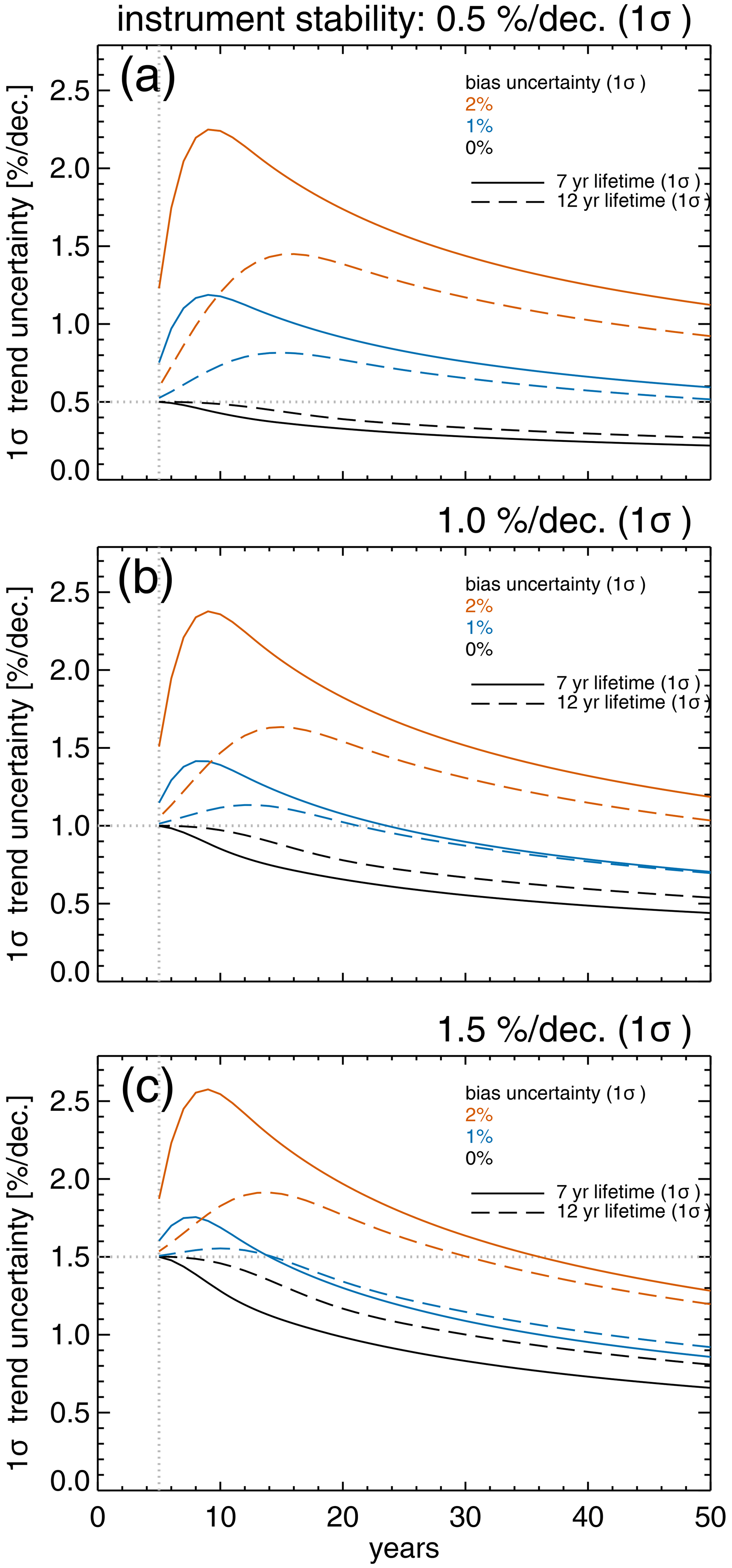
Figure 6Trend uncertainty in % per decade as a function of observation years for various stability requirements (a–c), different mean lifetimes of single satellite instruments (solid and dashed lines), and biases between consecutive observation systems (colors). Panels (a) to (c) show trend uncertainties for the 2σ GCOS-22 stability requirements of 1 % per decade (target), 2 % per decade (breakthrough), and 3 % per decade (threshold), respectively.
We present here a simple approach using Monte Carlo simulations to specifying stability requirements dependent on the need to observe a certain trend in merged datasets after a given period of time. Stratospheric ozone has been expected to recover since the end of the 1990s (somewhat less than 30 years ago), when stratospheric halogens released from ozone-depleting substances reached a maximum. While there are many possible combinations of satellite instruments, we show that a reasonable assumption of repeated single instruments with a mean lifetime of 7 years and a stability requirement of 3 % per decade (2σ) would yield a trend uncertainty of about 2 % per decade (2σ) after 30 years of observations. If the bias between consecutive observing systems is negligible due to a good bias correction in the case of a sufficient overlap between consecutive missions, the uncertainty improves to about 1.5 % per decade.
Our simple approach neglects the larger likelihood that instrument drifts with time are not necessarily linear nor are drifts normally distributed. The largest changes in satellite performance are usually in the beginning or near the end of the mission. When the ambient environment of a satellite instrument changes from the clean room on the ground to space conditions shortly after launch, calibration settings change, and if these changes are not adequately accounted for in the trace gas retrieval, they cause data drifts. In the first few years, instruments in space outgas, which changes the optical performance of the instrument more rapidly than in later years. In general, drifts can be caused by any changes in the optical performance (e.g., Bourassa et al., 2014). For limb-based satellite data, pointing errors to the tangent height can increase with time, particularly in the later part of the mission period (Bourassa et al., 2018). Near the end of the mission, instruments are aged and suffer from loss in thermal and/or power stability, which may again enhance the instrumental drift in the observational data.
The multiple merged satellite ozone data records are usually not entirely independent of each other, as the same satellite missions are used in different merged time series (e.g., Steinbrecht et al., 2017; SPARC/IO3C/GAW, 2019; Godin-Beekmann et al., 2022; Weber et al., 2022). In such a case, the trend uncertainty reduces more slowly than with , which is only valid for n truly independent time series.
Using a simple Monte Carlo time series simulation scheme, we were able to estimate the required stability of an observing instrument with a given lifetime that is needed to reach a certain trend uncertainty in a long-term time series consisting of series of satellites. This requirement depends on not only the length of the time series and lifetime, but also the biases between consecutive observing systems. The time range of the ozone recovery phase is now approaching 30 years in the next few years. With a typical mean lifetime of about 7 years for satellites, a 3 % per decade (2σ) stability (World Meteorological Organisation, 2022) adds about 1.5 % per decade (2σ) uncertainty to the statistical long-term trend uncertainty after 30 years.
Assuming a mean residual bias of about 1 % between consecutive measurement systems (after overlap corrections), the resulting long-term trend uncertainty increases to 2 % per decade. Combining the statistical (2 % per decade; Godin-Beekmann et al., 2022) and drift uncertainty (2 % per decade) as a Gaussian sum yields an overall trend uncertainty of about 3 % per decade, which is larger than the largest positive trends observed in the upper stratosphere (+2 % per decade). For total ozone with statistical trend uncertainties of about 0.5 % per decade (2σ), the total uncertainty is about 2 % per decade after 30 years. For long-term trend assessments, the current threshold requirement of 3 % per decade (2σ), as stated in World Meteorological Organisation (2022), is too high, and reducing it to 1 % per decade (2σ) is recommended.
For the next few decades, the long-term trend uncertainty will only decrease rather slowly, which means that redundancy in satellite instruments is very effective in reducing the impact from instrument drifts. Uncertainties due to instrument drifts can be cut nearly in half with three parallel satellites. All numbers provided here are lower limits since measurement errors as well as uncertainties due to data merging have not been accounted for.
Codes in IDL (Interactive Data Language) and simulated data are available upon request to the author.
The author is a member of the editorial board of Atmospheric Measurement Techniques. The peer-review process was guided by an independent editor, and the author also has no other competing interests to declare.
Publisher’s note: Copernicus Publications remains neutral with regard to jurisdictional claims made in the text, published maps, institutional affiliations, or any other geographical representation in this paper. While Copernicus Publications makes every effort to include appropriate place names, the final responsibility lies with the authors.
This work was carried out as part of the OREGANO (Ozone Recovery from Merged Observational Data and Model Analysis) project funded by the European Space Agency.
This research has been supported by the European Space Agency (grant no. 4000137112/22/I-AG) and by the State of Bremen via the University of Bremen.
The article processing charges for this open-access publication were covered by the University of Bremen.
This paper was edited by Gerrit Kuhlmann and reviewed by two anonymous referees.
Bourassa, A. E., Degenstein, D. A., Randel, W. J., Zawodny, J. M., Kyrölä, E., McLinden, C. A., Sioris, C. E., and Roth, C. Z.: Trends in stratospheric ozone derived from merged SAGE II and Odin-OSIRIS satellite observations, Atmos. Chem. Phys., 14, 6983–6994, https://doi.org/10.5194/acp-14-6983-2014, 2014. a, b
Bourassa, A. E., Roth, C. Z., Zawada, D. J., Rieger, L. A., McLinden, C. A., and Degenstein, D. A.: Drift-corrected Odin-OSIRIS ozone product: algorithm and updated stratospheric ozone trends, Atmos. Meas. Tech., 11, 489–498, https://doi.org/10.5194/amt-11-489-2018, 2018. a
CCI: Ozone cci – User Requirement Document (URD), Version 3.1, European Space Agency, https://climate.esa.int/media/documents/Ozone_cci_urd_v3.1_version_05032021.pdf (last access: 21 November 2023), 2021. a, b
CMUG: Climate Modelling User Group [CMUG] Deliverable 1.1, Meeting the needs of the Climate Community – Requirements, European Space Agency, https://admin.climate.esa.int/media/documents/CMUG_Baseline_Requirements_D1.1_v3.0.pdf (last access: 30 November 2023), 2022. a, b
Coldewey-Egbers, M., Loyola, D. G., Lerot, C., and Van Roozendael, M.: Global, regional and seasonal analysis of total ozone trends derived from the 1995–2020 GTO-ECV climate data record, Atmos. Chem. Phys., 22, 6861–6878, https://doi.org/10.5194/acp-22-6861-2022, 2022. a
Frith, S. M., Stolarski, R. S., Kramarova, N. A., and McPeters, R. D.: Estimating uncertainties in the SBUV Version 8.6 merged profile ozone data set, Atmos. Chem. Phys., 17, 14695–14707, https://doi.org/10.5194/acp-17-14695-2017, 2017. a
Godin-Beekmann, S., Azouz, N., Sofieva, V. F., Hubert, D., Petropavlovskikh, I., Effertz, P., Ancellet, G., Degenstein, D. A., Zawada, D., Froidevaux, L., Frith, S., Wild, J., Davis, S., Steinbrecht, W., Leblanc, T., Querel, R., Tourpali, K., Damadeo, R., Maillard Barras, E., Stübi, R., Vigouroux, C., Arosio, C., Nedoluha, G., Boyd, I., Van Malderen, R., Mahieu, E., Smale, D., and Sussmann, R.: Updated trends of the stratospheric ozone vertical distribution in the 60° S–60° N latitude range based on the LOTUS regression model, Atmos. Chem. Phys., 22, 11657–11673, https://doi.org/10.5194/acp-22-11657-2022, 2022. a, b, c, d, e, f
Guimaräes Couto, P. R., Carreteiro Damasceno, J., and Pinheiro de Oliveira, S.: Monte Carlo Simulations Applied to Uncertainty in Measurement, Chap. 2, IntechOpen Limited, 27–51, https://doi.org/10.5772/53014, 2013. a
Harris, N. R. P., Hassler, B., Tummon, F., Bodeker, G. E., Hubert, D., Petropavlovskikh, I., Steinbrecht, W., Anderson, J., Bhartia, P. K., Boone, C. D., Bourassa, A., Davis, S. M., Degenstein, D., Delcloo, A., Frith, S. M., Froidevaux, L., Godin-Beekmann, S., Jones, N., Kurylo, M. J., Kyrölä, E., Laine, M., Leblanc, S. T., Lambert, J.-C., Liley, B., Mahieu, E., Maycock, A., de Mazière, M., Parrish, A., Querel, R., Rosenlof, K. H., Roth, C., Sioris, C., Staehelin, J., Stolarski, R. S., Stübi, R., Tamminen, J., Vigouroux, C., Walker, K. A., Wang, H. J., Wild, J., and Zawodny, J. M.: Past changes in the vertical distribution of ozone – Part 3: Analysis and interpretation of trends, Atmos. Chem. Phys., 15, 9965–9982, https://doi.org/10.5194/acp-15-9965-2015, 2015. a
Hassler, B., Young, P. J., Ball, W. T., Damadeo, R., Keeble, J., Barras, E. M., Sofieva, V., and Zeng, G.: Update on Global Ozone: Past, Present, and Future, in: Scientific Assessment of Ozone Depletion: 2022, Chap. 3, World Meteorological Organization/UNEP, WMO GAW-58, https://library.wmo.int/idurl/4/58360 (last access: 11 June 2024), 2022. a, b, c
Hubert, D., Lambert, J.-C., Verhoelst, T., Granville, J., Keppens, A., Baray, J.-L., Bourassa, A. E., Cortesi, U., Degenstein, D. A., Froidevaux, L., Godin-Beekmann, S., Hoppel, K. W., Johnson, B. J., Kyrölä, E., Leblanc, T., Lichtenberg, G., Marchand, M., McElroy, C. T., Murtagh, D., Nakane, H., Portafaix, T., Querel, R., Russell III, J. M., Salvador, J., Smit, H. G. J., Stebel, K., Steinbrecht, W., Strawbridge, K. B., Stübi, R., Swart, D. P. J., Taha, G., Tarasick, D. W., Thompson, A. M., Urban, J., van Gijsel, J. A. E., Van Malderen, R., von der Gathen, P., Walker, K. A., Wolfram, E., and Zawodny, J. M.: Ground-based assessment of the bias and long-term stability of 14 limb and occultation ozone profile data records, Atmos. Meas. Tech., 9, 2497–2534, https://doi.org/10.5194/amt-9-2497-2016, 2016. a
Rahpoe, N., Weber, M., Rozanov, A. V., Weigel, K., Bovensmann, H., Burrows, J. P., Laeng, A., Stiller, G., von Clarmann, T., Kyrölä, E., Sofieva, V. F., Tamminen, J., Walker, K., Degenstein, D., Bourassa, A. E., Hargreaves, R., Bernath, P., Urban, J., and Murtagh, D. P.: Relative drifts and biases between six ozone limb satellite measurements from the last decade, Atmos. Meas. Tech., 8, 4369–4381, https://doi.org/10.5194/amt-8-4369-2015, 2015. a
SPARC/IO3C/GAW: SPARC/IO3C/GAW Report on Long-term Ozone Trends and Uncertainties in the Stratosphere, edited by: Petropavlovskikh, I., Godin-Beekmann, S., Hubert, D., Damadeo, R., Hassler, B., and Sofieva, V., SPARC Report No. 9, GAW Report No. 241, WCRP-17/2018, https://doi.org/10.17874/f899e57a20b, 2019. a, b, c
Steinbrecht, W., Froidevaux, L., Fuller, R., Wang, R., Anderson, J., Roth, C., Bourassa, A., Degenstein, D., Damadeo, R., Zawodny, J., Frith, S., McPeters, R., Bhartia, P., Wild, J., Long, C., Davis, S., Rosenlof, K., Sofieva, V., Walker, K., Rahpoe, N., Rozanov, A., Weber, M., Laeng, A., von Clarmann, T., Stiller, G., Kramarova, N., Godin-Beekmann, S., Leblanc, T., Querel, R., Swart, D., Boyd, I., Hocke, K., Kämpfer, N., Maillard Barras, E., Moreira, L., Nedoluha, G., Vigouroux, C., Blumenstock, T., Schneider, M., García, O., Jones, N., Mahieu, E., Smale, D., Kotkamp, M., Robinson, J., Petropavlovskikh, I., Harris, N., Hassler, B., Hubert, D., and Tummon, F.: An update on ozone profile trends for the period 2000 to 2016, Atmos. Chem. Phys., 17, 10675–10690, https://doi.org/10.5194/acp-17-10675-2017, 2017. a, b
United Nations: VIENNA: The Vienna Convention for the Protection of the Ozone Layer, United Nations, https://treaties.un.org/doc/Treaties/1988/09/19880922%2003-14%20AM/Ch_XXVII_02p.pdf (last access: 12 June 2024), 1985. a
Veefkind, J., Aben, I., McMullan, K., Förster, H., de Vries, J., Otter, G., Claas, J., Eskes, H., de Haan, J., Kleipool, Q., van Weele, M., Hasekamp, O., Hoogeveen, R., Landgraf, J., Snel, R., Tol, P., Ingmann, P., Voors, R., Kruizinga, B., Vink, R., Visser, H., and Levelt, P.: TROPOMI on the ESA Sentinel-5 Precursor: A GMES mission for global observations of the atmospheric composition for climate, air quality and ozone layer applications, Remote Sens. Environ., 120, 70–83, https://doi.org/10.1016/j.rse.2011.09.027, 2012. a
Weatherhead, E. C., Reinsel, G. C., Tiao, G. C., Meng, X.-L., Choi, D., Cheang, W.-K., Keller, T., DeLuisi, J., Wuebbles, D. J., Kerr, J. B., Miller, A. J., Oltmans, S. J., and Frederick, J. E.: Factors affecting the detection of trends: Statistical considerations and applications to environmental data, J. Geophys. Res.-Atmos., 103, 17149–17161, https://doi.org/10.1029/98JD00995, 1998. a
Weatherhead, E. C., Harder, J., Araujo-Pradere, E. A., Bodeker, G., English, J. M., Flynn, L. E., Frith, S. M., Lazo, J. K., Pilewskie, P., Weber, M., and Woods, T. N.: How long do satellites need to overlap? Evaluation of climate data stability from overlapping satellite records, Atmos. Chem. Phys., 17, 15069–15093, https://doi.org/10.5194/acp-17-15069-2017, 2017. a, b, c
Weber, M., Coldewey-Egbers, M., Fioletov, V. E., Frith, S. M., Wild, J. D., Burrows, J. P., Long, C. S., and Loyola, D.: Total ozone trends from 1979 to 2016 derived from five merged observational datasets – the emergence into ozone recovery, Atmos. Chem. Phys., 18, 2097–2117, https://doi.org/10.5194/acp-18-2097-2018, 2018. a
Weber, M., Arosio, C., Coldewey-Egbers, M., Fioletov, V. E., Frith, S. M., Wild, J. D., Tourpali, K., Burrows, J. P., and Loyola, D.: Global total ozone recovery trends attributed to ozone-depleting substance (ODS) changes derived from five merged ozone datasets, Atmos. Chem. Phys., 22, 6843–6859, https://doi.org/10.5194/acp-22-6843-2022, 2022. a, b, c, d, e, f
World Meteorological Organisation: GCOS-01: WMO/CEOS report on a strategy for integrating satellite and ground-based observations of ozone, WMO GAW-140, World Meteorological Organisation, https://library.wmo.int/idurl/4/36995 (last access: 21 November 2023), 2001. a, b, c
World Meteorological Organisation: IGACO-04: The Changing Atmosphere – An Integrated Global Atmospheric Chemistry Observation Theme for the IGOS Partnership, WMO GAW-159, ESA SP-1282, World Meteorological Organisation, https://library.wmo.int/idurl/4/41238 (last access: 11 June 2024), 2004. a
World Meteorological Organisation: GCOS-11: Systematic Observation Requirements for Satellite-based Products for Climate Supplemental details to the satellite-based component of the Implementation Plan for the Global Observing System for Climate in Support of the UNFCCC – 2011 update, WMO GCOS-254, World Meteorological Organisation, https://library.wmo.int/idurl/4/48411 (last access: 1 December 2023), 2011. a
World Meteorological Organisation: GCOS-22: The 2022 GCOS ECVs Requirements, WMO GCOS-245, World Meteorological Organisation, https://library.wmo.int/idurl/4/58111 (last access: 21 November 2023), 2022. a, b, c, d, e
Zerefos, C., Fountoulakis, I., Eleftheratos, K., and Kazantzidis, A.: Long-term variability of human health-related solar ultraviolet-B radiation doses from the 1980s to the end of the 21st century, Physiol. Rev., 103, 1789–1826, https://doi.org/10.1152/physrev.00031.2022, 2023. a