Deriving cloud droplet number concentration from surface-based remote sensors with an emphasis on lidar measurements

Given the importance of constraining cloud droplet number concentrations (N_d) in low-level clouds, we explore two methods for retrieving N_d from surface-based remote sensing that emphasize the information content in lidar measurements. Because N_d is the zeroth moment of the droplet size distribution (DSD), and all remote sensing approaches respond to DSD moments that are at least 2 orders of magnitude greater than the zeroth moment, deriving N_d from remote sensing measurements has significant uncertainty. At minimum, such algorithms require the extrapolation of information from two other measurements that respond to different moments of the DSD. Lidar, for instance, is sensitive to the second moment (cross-sectional area) of the DSD, while other measures from microwave sensors respond to higher-order moments. We develop methods using a simple lidar forward model that demonstrates that the depth to the maximum in lidar-attenuated backscatter (R_max) is strongly sensitive to N_d when some measure of the liquid water content vertical profile is given or assumed. Knowledge of R_max to within 5 m can constrain N_d to within several tens of percent. However, operational lidar networks provide vertical resolutions of > 15 m, making a direct calculation of N_d from R_max very uncertain. Therefore, we develop a Bayesian optimal estimation algorithm that brings additional information to the inversion such as lidar-derived extinction and radar reflectivity near the cloud top. This statistical approach provides reasonable characterizations of N_d and effective radius (r_e) to within approximately a factor of 2 and 30 %, respectively. By comparing surface-derived cloud properties with MODIS satellite and aircraft data collected during the MARCUS and CAPRICORN II campaigns, we demonstrate the utility of the methodology.

1 Introduction

The number of cloud droplets per unit volume (N_d) is essential for characterizing cloud properties. Particularly for lower-tropospheric liquid-phase clouds, N_d forms a bridge between atmospheric aerosol and the Earth's albedo by determining how condensed water is partitioned into droplet surface area. Higher droplet concentrations for a given condensed mass result in more surface area and more reflective clouds (Twomey, 1974). Thus, many cloud parameterizations used in models include N_d as one of the moments in multi-moment cloud schemes where the other moment is typically related to the mass mixing ratio (Gettelman and Morrison, 2015; Thompson and Eidhammer, 2014; Seifert and Beheng, 2005). Conceptually, using N_d as a baseline parameter makes sense since droplets typically condense on hygroscopic aerosol particles (hereafter cloud condensation nuclei or CCN), thereby fixing N_d as the water droplets grow in an updraft. The initial N_d at the cloud base would be an upper limit on N_d in the ascending updraft because coalescence processes would reduce N_d, and precipitation would further scavenge cloud droplets. However, aircraft observations often show that for shallow clouds less than 1 km in depth with minimal precipitation, N_d is reasonably constant with height (Miles et al., 2000) and strongly correlated with CCN (McFarquhar et al., 2021).

In this paper, we revisit the methodology used in Mace et al. (2021; hereafter M21) and attempt to extend that methodology with a focus on lidar measurements from below the cloud. In M21, a method derived therein was applied to non-precipitating clouds For which the layer-averaged radar reflectivity provided the primary source of information. While M21 used the lidar measurements at the cloud base to contribute to the first guess, M21 did not fully exploit the information content available in the lidar measurements. Here, we more thoroughly examine what the lidar signal near the cloud base can tell us about cloud properties in optically thick boundary layer clouds. Because the lidar backscatter is much larger at the cloud base than in subcloud drizzle, we apply the methodology to lightly precipitating and non-precipitating clouds.

2 Methods

2.1 Instruments and comparison approach

We focus on data collected during the summer of 2018 from two ship-based campaigns on the Australian research vessel (R/V) Investigator and the Australian icebreaker Aurora Australis during voyages between Hobart, Australia, and East Antarctica. These campaigns are known, respectively, as the second Clouds, Aerosols, Precipitation, Radiation and atmospheric Composition Over the SoutheRn Ocean (CAPRICORN II) and Measurements of Aerosols, Radiation, and Clouds over the Southern Ocean (MARCUS). These campaigns and a detailed accounting of instrumentation are described in McFarquhar et al. (2021) and Mace et al. (2021).

The key observations we focus on in this paper are vertically pointing depolarization elastic-backscatter lidars, vertically pointing W-band radars, microwave radiometers, and ancillary measurements provided by radiosondes and surface meteorological instruments. This combination of active and passive instruments (radar, lidar, and radiometer) have become common in many cloud- and precipitation-focused field campaigns and enable the derivation of cloud properties as described herein. One important synergy in this instrument suite is that the lidar is very sensitive to the droplets at cloud base, while the radar is most sensitive to the cloud-top region where the droplets are largest in non-precipitating clouds, thereby providing immediate information on cloud layer depth. In terms of the measurable quantities, the lidar-attenuated backscatter measurement is sensitive to the second moment of the droplet size distribution (DSD), the radar to the sixth moment of the DSD, and the microwave radiometer to the integrated condensed mass in the vertical column (liquid water path or LWP, hereafter). For non-precipitating clouds, Frisch et al. (1998) illustrate how the radar reflectivity profile, being proportional to the square of the condensed mass, can be cast as a weighting function to vertically distribute the LWP. The lidar then, being the most sensitive to the smaller droplets that compose the DSD, provides information regarding how the mass is distributed into the droplets. Combining the layer depth information and the LWP, we have immediate and critical information regarding the degree of adiabaticity of the layer (Albrecht et al., 1990). We seek to exploit these synergies in the algorithms described in the following sections.

While we focus on the information in surface-based measurements, we also take advantage of airborne in situ measurements and measurements provided by satellites. Again, with a theme of synergy, in situ data provide a direct measure of the cloud properties we seek to infer from remote sensing measurements in unique and rare instances of coordination, while the satellite data provide regional observations from frequently occurring overpasses. The satellite overpasses over periods of weeks to months provide good coverage of diverse cloud fields collected over the course of a campaign. We make use of these additional platforms to both validate our algorithms but also to provide context and understanding of the processes at work in a particular cloud field.

2.2 Theory and assumptions

The observed lidar-attenuated backscatter β_obs can be combined with other measurements to derive N_d in fully attenuating liquid-phase clouds when measured from the surface. Even though light precipitation may be present, we assume that β_obs is dominated by a droplet distribution (N(D)) that is describable by a modified gamma function. Following Appendix B in Posselt and Mace (2014),

$$\begin{array}{}\text{(1)}& {\displaystyle \frac{\mathrm{d}N\left(D\right)}{\mathrm{d}D}}=N_{\mathrm{0}}{\left({\displaystyle \frac{D}{D_{\mathrm{0}}}}\right)}^{\mathit{\alpha }}\exp \left(-{\displaystyle \frac{D}{D_{\mathrm{0}}}}\right),\end{array}$$

where $\frac{\mathrm{d}N\left(D\right)}{\mathrm{d}D}$ is the droplet number concentration per unit size D (with units of cm⁻⁴ in the centimeter–gram–second (cgs) unit system). N₀ (with units of cm⁻⁴), D₀ (with units of cm), and α (unitless) are, respectively, the characteristic number, diameter, and the shape parameter of the N(D) distribution function. This simple integrable function allows us to express the microphysical quantities, N_d, q (liquid water content), r_e (effective radius), σ (extinction), and Z (radar reflectivity in the Rayleigh limit), with the following expressions by integrating over all D:

$$\begin{array}{}\text{(2)}& {\displaystyle }{N}_{\mathrm{d}}=N_{\mathrm{0}}{D}_{\mathrm{0}}\mathrm{\Gamma }\left(\mathit{\alpha }+\mathrm{1}\right)\text{(3)}& {\displaystyle }q=\mathit{\rho }{\displaystyle \frac{\mathit{\pi }}{\mathrm{6}}}{N}_{\mathrm{0}}{D}_{\mathrm{0}}^{\mathrm{4}}\mathrm{\Gamma }\left(\mathit{\alpha }+\mathrm{4}\right)\text{(4)}& {\displaystyle }{r}_{\mathrm{e}}={\displaystyle \frac{D_{\mathrm{0}}}{\mathrm{2}}}\left(\mathit{\alpha }+\mathrm{3}\right)\text{(5)}& {\displaystyle }\mathit{\sigma }={\displaystyle \frac{\mathit{\pi }}{\mathrm{2}}}{N}_{\mathrm{0}}{D}_{\mathrm{0}}^{\mathrm{3}}\mathrm{\Gamma }\left(\mathit{\alpha }+\mathrm{3}\right)\text{(6)}& {\displaystyle }Z=N_{\mathrm{0}}{D}_{\mathrm{0}}^{\mathrm{7}}\mathrm{\Gamma }\left(\mathit{\alpha }+\mathrm{7}\right),\end{array}$$

where ρ is the density of liquid water, and Γ is the gamma function. r_e is derived as the ratio of the third moment of N(D) to the second moment of N(D), followed by application of the recursion relationship of the gamma function. For σ, we assume that the extinction efficiency can be approximated as 2 for integrations over typical water droplet distributions. The radar reflectivity Z is written as the sixth moment of the DSD consistent with the Rayleigh approximation, which is valid for cloud droplets and radar wavelengths up to the W band (∼ 94 GHz or ∼ 3 mm wavelength). Conversion from conventional units (of mm⁶ m⁻³) to units in the cgs system (cm³) requires the multiplication of Z by 10⁻¹². Using Eqs. (2)–(6), we develop relationships among the variables as follows:

$$\begin{array}{}\text{(7)}& {\displaystyle }{N}_{\mathrm{d}}={\displaystyle \frac{\mathrm{3}}{\mathrm{4}}}{\displaystyle \frac{\mathrm{1}}{k\mathit{\pi }\mathit{\rho }}}{\displaystyle \frac{q}{r_{\mathrm{e}}^{\mathrm{3}}}},\text{(8)}& {\displaystyle }Z=q{r}_{\mathrm{e}}^{\mathrm{3}}C,\text{(9)}& {\displaystyle }\mathit{\sigma }={\displaystyle \frac{\mathrm{3}}{\mathrm{2}\mathit{\rho }}}{\displaystyle \frac{q}{r_{\mathrm{e}}}},\end{array}$$

where $k=\frac{(\mathit{\alpha }+\mathrm{2})(\mathit{\alpha }+\mathrm{1})}{(\mathit{\alpha }+\mathrm{3}{)}^{\mathrm{2}}}$, and $C=\frac{\mathrm{48}\mathrm{\Gamma }(\mathit{\alpha }+\mathrm{7})}{\mathit{\pi }\mathrm{\Gamma }(\mathit{\alpha }+\mathrm{4})(\mathit{\alpha }+\mathrm{3}{)}^{\mathrm{3}}}$. Equation (9) was first derived by Stephens (1978) and illustrates a pathway to deriving N_d from multispectral satellite reflectance measurements. For instance, the bispectral method applied to MODIS (Nakajima and King, 1990; Platnick et al., 2003) returns measurements of optical depth (τ) and r_e. Since τ is the vertical integral of σ, Eq. (3) can be adapted for use with satellite retrievals. A full derivation and error analysis of deriving N_d and other quantities from bispectral satellite retrievals is presented in Grosvenor et al. (2018; hereafter G18).

Following Platt (1977), and extending through the work of Hu et al. (2007) and Li et al. (2011) among others, we express the observed lidar-attenuated backscatter as

$$\begin{array}{}\text{(10)}& {\mathit{\beta }}_{\mathrm{obs}}\left(R\right)=\mathit{\beta }\left(R\right)e^{-\mathrm{2}\int \mathit{\eta }\mathit{\sigma }\mathrm{d}R}.\end{array}$$

β_obs is the result of two-way attenuation through the cloud to a point R (range) in the layer, and σ is the extinction coefficient with units of inverse length where σ is expressed in terms of the lidar ratio, $S=\frac{\mathit{\sigma }}{\mathit{\beta }}$. A factor η hereafter referred to as the multiple scattering factor accounts for the addition of photons to the observed signal due to multiple scattering in optically dense clouds. Defining the layer-integrated total attenuated backscatter as $\mathit{\gamma }=\int {\mathit{\beta }}_{\parallel +\perp }$ and the layer-integrated depolarization ratio as $\mathit{\delta }=\frac{\int {\mathit{\beta }}_{\perp }}{\int {\mathit{\beta }}_{\parallel +\perp }}$, we express $\mathit{\eta }={\left(\frac{\mathrm{1}-\mathit{\delta }}{\mathrm{1}+\mathit{\delta }}\right)}^{\mathrm{2}}$ (Hu et al., 2009). Platt et al. (1999) relate S with η, according to $S\mathit{\eta }=\frac{\mathrm{1}-T^{\mathrm{2}}}{\mathrm{2}\mathit{\gamma }}$, where T is the layer transmittance. When the layer is fully attenuating (T = 0), $S=\frac{\mathrm{1}}{\mathrm{2}\mathit{\eta }\mathit{\gamma }}$.

Figure 1 illustrates two examples of β_obs profiles measured by a micropulse lidar (Lewis et al., 2020) on board the Aurora Australis during MARCUS. Note that the units of the lidar signal in Fig. 1 are expressed as normalized relative backscatter (NRB) in Fig. 1 that is equivalent to β_obs via a calibration constant. We convert NRB to β_obs using a calibration technique described in O'Connor et al. (2004). We see the typically small β_obs below the cloud that is due to aerosol and molecular scattering in Fig. 1a, while in Fig. 1b, there is a contribution from drizzle (observed by a collocated W-band radar; not shown). There is an immediate increase in β_obs at a height where condensed liquid water droplets near the cloud base activate, grow rapidly with height, and begin to dominate the lidar signal scattering. β_obs then increases exponentially, according to Eq. (4), until the two-way attenuation causes β_obs to reach a maximum value which decays exponentially. We define the range from cloud base to the maximum in β_obs as R_max. Beyond R_max, β_obs gains more contribution by multiple-scattered light, depending on the lidar field of view, and in liquid clouds, the signal becomes increasingly depolarized relative to the transmitted signal because the orientation of the electric field vector is modified by the directionality of each scattering event. The progressive depolarization of the scattered signal is a function of the droplet size distribution (Hu et al., 2009). The overall result is quantified by η, which is a factor of less than 1 that effectively adds signal to β_obs in Eq. (10). The logarithmic decay of β_obs was shown by Li et al. (2011) to be related to σ as follows:

$$\begin{array}{}\text{(11)}& \mathit{\eta }\mathit{\sigma }=-{\displaystyle \frac{\ln \mathit{\beta }{\left(R_{\mathrm{2}}\right)}_{\mathrm{obs}}-\ln \mathit{\beta }{\left(R_{\mathrm{1}}\right)}_{\mathrm{obs}}}{\mathrm{2}\left(R_{\mathrm{2}}-R_{\mathrm{1}}\right)}},\end{array}$$

where (r₂−r₁) is the range over which the change in β_obs is calculated. Because we have estimated η from measurements, we can estimate σ in the optically thick part of the layer beyond the peak in β_obs using linear regression. Li et al. (2011) compare σ derived from this method to estimates of σ derived from passive reflectances and find an uncertainty of ∼ 13 %, although we assume it to be higher (20 %) below. This method's accuracy depends on calculating the rate at which the signal decays with depth in the layer. In practice, we fit a regression line to β_obs at ranges beyond R_max until the signal is a factor of 2 above the lidar noise floor. We determine the lidar noise level from the mean β_obs well beyond the point of full attenuation in the cloud layer. The goodness of the linear regression fit depends on the number of measurements in this range where the signal is decaying. The accuracy depends on the vertical resolution of the lidar measurements for a given σ. The accuracy of the fit is tracked and used to estimate uncertainty.

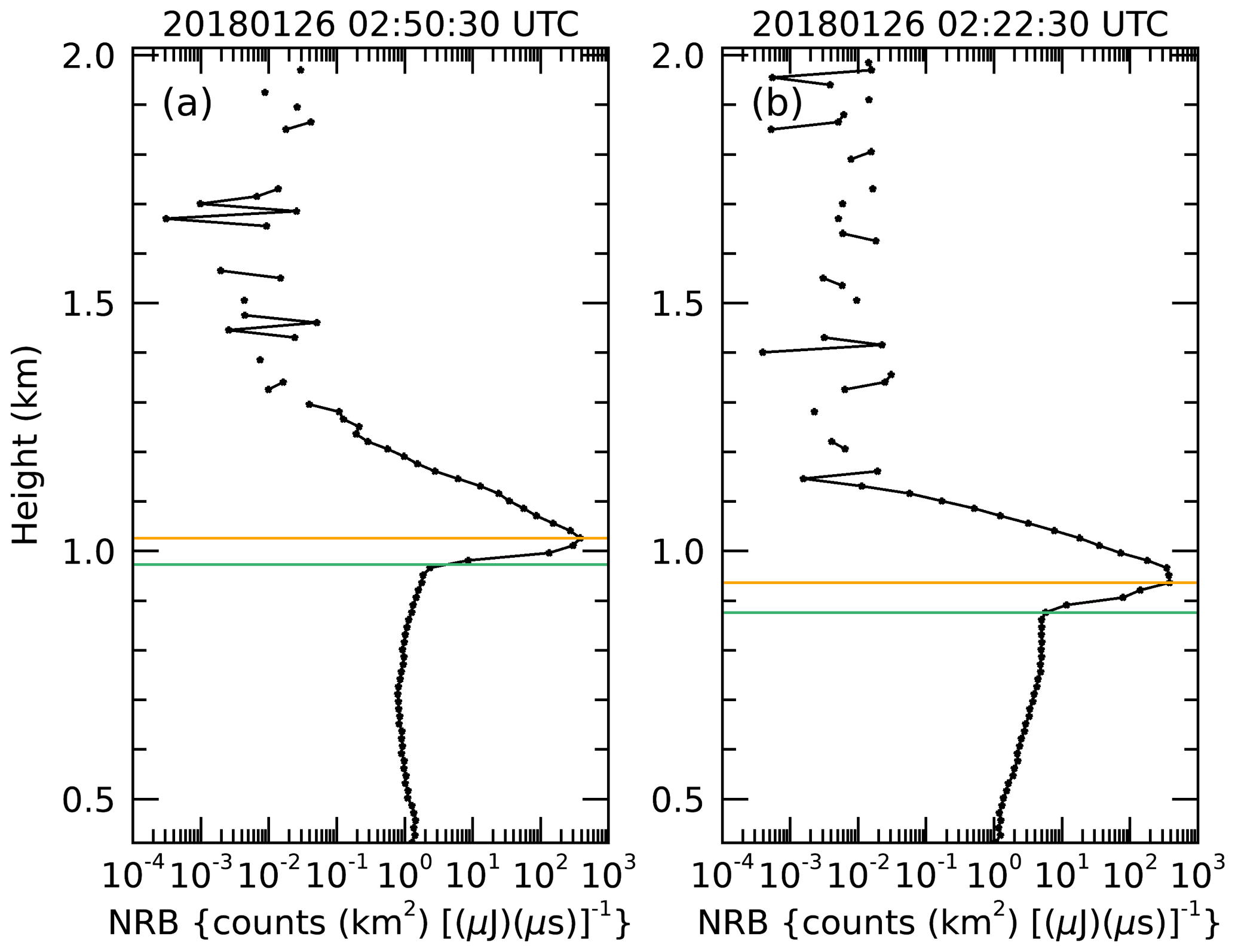
Figure 1 Two examples of normalized relative backscatter (NRB; Campbell et al., 2002) from micropulse lidar data collected during MARCUS on 26 January 2018. Panel (a) shows a profile in a non-drizzling cloud collected at 02:50:30 UTC. Panel (b) shows a profile collected at 02:22:30 UTC that had subcloud drizzle, as indicated by the cloud radar. The green line indicates the height determined to be cloud base, while the red line indicate the maximum in β_obs. The distance between the green and red lines is defined as R_max.

2.3 Direct calculation of N_d and r_e

The growth of the lidar signal from cloud base to R_max can be used to gain information about the cloud layer. Taking the natural logarithm of both sides of Eq. (10), recognizing that βS_c=σ, and then differentiating with range r in the cloud layer, we can write

$$\begin{array}{}\text{(12)}& {\displaystyle \frac{\partial \ln {\mathit{\beta }}_{\mathrm{obs}}}{\partial R}}={\displaystyle \frac{\partial \ln \mathit{\sigma }}{\partial R}}-\mathrm{2}\mathit{\eta }\mathit{\sigma }.\end{array}$$

We next derive an expression relating σ in terms of N_d and q. We can simply express N₀ in terms of N_d, as $N_{\mathrm{0}}=\frac{N_{\mathrm{d}}}{{\mathrm{D}}_{\mathrm{0}}\mathrm{\Gamma }\left(\mathit{\alpha }+\mathrm{1}\right)}$, and substitute it into Eq. (5) as

$$\begin{array}{}\text{(13)}& \mathit{\sigma }={\displaystyle \frac{\mathit{\pi }}{\mathrm{2}}}{\displaystyle \frac{N_{\mathrm{d}}}{\mathrm{\Gamma }\left(\mathit{\alpha }+\mathrm{1}\right)}}{D}_{\mathrm{0}}^{\mathrm{2}}\mathrm{\Gamma }\left(\mathit{\alpha }+\mathrm{3}\right).\end{array}$$

Then we solve the expression for σ in Eq. (5) for D₀, where $D_{\mathrm{0}}^{\mathrm{3}}=\frac{\mathit{\sigma }}{\frac{\mathit{\pi }}{\mathrm{2}}{N}_{\mathrm{0}}\mathrm{\Gamma }(\mathit{\alpha }+\mathrm{3})}$, then substitute it into Eq. (3), and rearrange it to obtain $D_{\mathrm{0}}=\frac{\mathrm{3}}{\mathit{\rho }}\frac{q}{\mathit{\sigma }}\frac{\mathrm{\Gamma }(\mathit{\alpha }+\mathrm{3})}{\mathrm{\Gamma }(\mathit{\alpha }+\mathrm{4})}$. Now substitute the expression for D₀ into Eq. (13) and rearrange as follows:

$$\begin{array}{}\text{(14)}& \mathit{\sigma }=N_{\mathrm{d}}^{\frac{\mathrm{1}}{\mathrm{3}}}{q}^{\frac{\mathrm{2}}{\mathrm{3}}}B,\end{array}$$

where $B={\left(\frac{\mathrm{9}\mathit{\pi }}{\mathrm{2}{\mathit{\rho }}^{\mathrm{2}}}\frac{\left[\mathrm{\Gamma }\right(\mathit{\alpha }+\mathrm{3}){]}^{\mathrm{3}}}{\left[\mathrm{\Gamma }\right(\mathit{\alpha }+\mathrm{4}\left){]}^{\mathrm{2}}\mathrm{\Gamma }\right(\mathit{\alpha }+\mathrm{1})}\right)}^{\frac{\mathrm{1}}{\mathrm{3}}}$ collects constants and assumptions. Now we combine Eqs. (12) and (14):

$${\displaystyle \frac{\mathrm{d}\ln \left({\mathit{\beta }}_{\mathrm{obs}}\right)}{\mathrm{d}r}}={\displaystyle \frac{B{N}_{\mathrm{d}}^{\frac{\mathrm{1}}{\mathrm{3}}}}{\mathit{\sigma }}}{\displaystyle \frac{\mathrm{d}}{\mathrm{d}r}}\left(q^{\frac{\mathrm{2}}{\mathrm{3}}}\right)-\mathrm{2}\mathit{\eta }\mathit{\sigma }.$$

Solving the derivative for q,

$${\displaystyle \frac{\mathrm{d}}{\mathrm{d}r}}\left(q^{\frac{\mathrm{2}}{\mathrm{3}}}\right)={\displaystyle \frac{\mathrm{2}}{\mathrm{3}}}{q}^{-\frac{\mathrm{1}}{\mathrm{3}}}{\displaystyle \frac{\mathrm{d}q}{\mathrm{d}r}},$$

substituting into Eq. (14), and then, when simplifying, we arrive at

$${\displaystyle \frac{\mathrm{d}\ln \left({\mathit{\beta }}_{\mathrm{obs}}\right)}{\mathrm{d}r}}={\displaystyle \frac{\mathrm{2}}{\mathrm{3}}}{\displaystyle \frac{\mathrm{d}\ln q}{\mathrm{d}r}}-\mathrm{2}B\mathit{\eta }{N}_{\mathrm{d}}^{\frac{\mathrm{1}}{\mathrm{3}}}{q}^{\frac{\mathrm{2}}{\mathrm{3}}},$$

and then solve for N_d as follows:

$$\begin{array}{}\text{(15)}& N_{\mathrm{d}}^{\frac{\mathrm{1}}{\mathrm{3}}}={\displaystyle \frac{\frac{\mathrm{2}}{\mathrm{3}}\frac{\mathrm{d}\ln q}{\mathrm{d}R}-\frac{\mathrm{d}\ln \left({\mathit{\beta }}_{\mathrm{obs}}\right)}{\mathrm{d}r}}{\mathrm{2}B\mathit{\eta }{q}^{\frac{\mathrm{2}}{\mathrm{3}}}}}.\end{array}$$

Since q=f_adΓ_lR, where Γ_l is the layer mean adiabatic liquid water lapse rate that depends on temperature and pressure and the moist adiabatic lapse rate (G18), we substitute into Eq. (15); noting that $\frac{\mathrm{d}\ln q}{\mathrm{d}R}=\frac{\mathrm{1}}{R}$, we can write Eq. (15) as

$$\begin{array}{}\text{(16)}& N_{\mathrm{d}}={\left({\displaystyle \frac{\frac{\mathrm{2}}{\mathrm{3}r}-\frac{\mathrm{d}\ln {\mathit{\beta }}_{\mathrm{obs}}}{\mathrm{d}r}}{\mathrm{2}\mathit{\eta }{\left({\mathrm{\Gamma }}_{l}R{f}_{\mathrm{ad}}\right)}^{\frac{\mathrm{2}}{\mathrm{3}}}B}}\right)}^{\mathrm{3}}.\end{array}$$

Now where $\frac{\mathrm{d}\ln \left({\mathit{\beta }}_{\mathrm{obs}}\right)}{\mathrm{d}r}=\mathrm{0}$ at R_max, we simplify the expression to arrive at

$$\begin{array}{}\text{(17)}& N_{\mathrm{d}}={\displaystyle \frac{\mathrm{1}}{\mathrm{27}{B}^{\mathrm{3}}{\mathit{\eta }}^{\mathrm{3}}{\mathrm{\Gamma }}_l^{\mathrm{2}}{R}_{max}^{\mathrm{5}}{f}_{\mathrm{ad}}^{\mathrm{2}}}}.\end{array}$$

In Eq. (17), N_d is a function of observable quantities with an assumption that the liquid water profile has an adiabatic shape. The DSD shape parameter α is also assumed and typically given a value that conforms to in situ data (see below). f_ad, which scales the adiabatic liquid water content, can be calculated as the ratio of the vertically integrated liquid water mass or liquid water path (LWP) that is readily retrieved from measurements collected by a microwave radiometer (Turner et al., 2016) to the adiabatic LWP that can be derived by integrating Γ_l over the depth of the layer (G18). The depth of the layer must be determined from some means such as a vertically pointing cloud radar or perhaps from recent radiosonde soundings. Thus, N_d can be derived with a combination of a depolarization lidar, some means of determining cloud top, and a microwave radiometer. Neither the lidar nor the radar, if present, must be calibrated to derive N_d with Eq. (17). With LWP and N_d and a measure of layer depth, it is straightforward to estimate a characteristic cloud droplet size. Typically, the cloud-top r_e is most representative of the layer reflectance and is derived from bispectral measurements such as MODIS (to which we will compare later). Following G18,

$$\begin{array}{}\text{(18)}& r_{\mathrm{e}}={\left({\displaystyle \frac{\frac{\mathrm{3}h}{\mathrm{4}\mathit{\pi }{\mathit{\rho }}_l}{\mathrm{\Gamma }}_l{f}_{\mathrm{ad}}}{k{N}_{\mathrm{d}}}}\right)}^{\mathrm{1}/\mathrm{3}},\end{array}$$

where h is the layer thickness, and k is the cubed ratio of a volume-weighted characteristic droplet size to the effective droplet size assumed constant at 0.8.

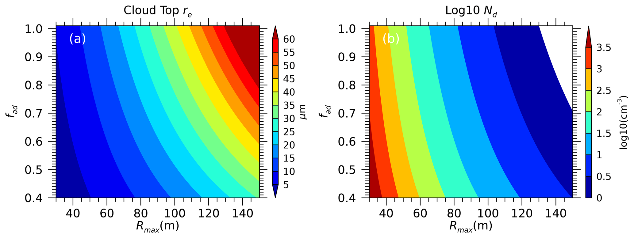
Figure 2 Response of Eq. (18) (a; r_e) and Eq. (17) (b; N_d) to typical values of R_max and f_ad.

Figure 2 shows the response of Eqs. (17) and (18) to typical ranges of R_max and f_ad. In these calculations, we fix η at 0.4 (a typical value for the lidar on CAPRICORN II) and the cloud layer thickness at 500 m. We find that R_max contributes most significantly to the N_d calculation, given the fifth power exponent in the denominator of Eq. (17). N_d ranges from near 1000 cm⁻³ for low R_max values that would correspond to very opaque layers to values smaller than 10 cm⁻³ for layers with R_max exceeding 100 m. These correspond to the approximate typical extremes for R_max found in measurements. r_e ranges from 5 µm for small R_max to more than 50 µm for very large R_max, corresponding to the change in N_d from high to low, respectively. For a given R_max, an increasingly adiabatic cloud layer causes N_d to decrease and r_e to increase. This tendency makes physical sense, since, for our simple conceptual model of an adiabatically increasing q profile, increasing f_ad for a given LWP and layer thickness (h) implies more liquid water in the profile. Therefore, for a given R_max, fewer but larger droplets are required to achieve a given extinction profile that allows the lidar beam to penetrate the layer.

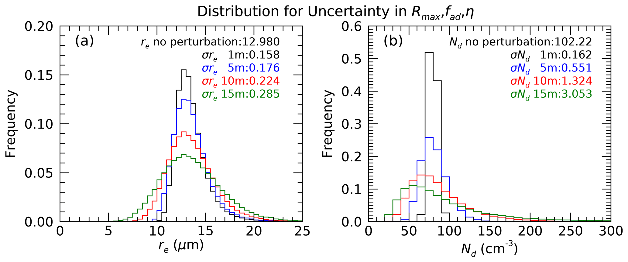
Figure 3 Sensitivity of Eq. (17) (a) and Eq. (18) (b) to the uncertainty in input parameters. The insets list the resulting uncertainties corresponding to the color-coded frequency distributions. The insets list the normalized standard deviations for an assumed standard deviation in R_max of 1, 5, 10, and 15 m. The lidar range gate spacing would be twice the standard deviation in R_max.

While Eqs. (17) and (18) produce physically plausible results, as illustrated in Fig. 2, the sensitivity of N_d to the uncertainty in R_max is substantial. The resulting uncertainty in N_d then translates into uncertainty in r_e. Clearly, with the typical range in R_max between a few tens of meters to values not much greater than about 100 m, the vertical resolution of the lidar has a significant bearing on how well we can know R_max. Lidars in operational networks typically operate with range bin spacing of between 10 and 15 m. The micropulse lidars operated by the U.S. Department of Energy (DOE) Atmospheric Radiation Measurement (ARM) program (Mather, 2021) use 15 m spacing, while Vaisala laser ceilometers use a range bin spacing of 10 m. We use a bootstrap approach to evaluate the effect of this uncertainty in R_max. We assume that the 1 standard deviation of uncertainty in R_max would be half of the range bin spacing. Fixing the uncertainty in f_ad and η at 20 % and allowing a variable R_max uncertainty of 1, 5, 10, and 15 m, we use a normally distributed set of random numbers to perturb the R_max, f_ad, and η about their assumed values prior to the implementation of Eqs. (9) and (10). In total, 25 000 iterations are used to compute the frequency distribution of the resulting N_d and r_e (Fig. 3) for each R_max uncertainty. We find that range bin spacing in excess of 10 m is inadequate for calculating N_d. A 30 m range bin spacing results in a normalized standard deviation in the N_d distribution for the example shown here of ∼ 3. The r_e normalized standard deviation is approximately 29 % in this case. The uncertainty in N_d and r_e decreases as the uncertainty in R_max is reduced from 15 to 1 m. At 1 and 5 m uncertainty in R_max corresponding to 2 and 10 m range bin spacing, N_d (r_e) has fractional uncertainties of 0.16 (0.16) and 0.55 (0.18), respectively. These levels of uncertainty would convey useful information about a cloud layer, although the magnitude of the uncertainty as illustrated by the frequency distribution (blue) in Fig. 3 illustrates that the uncertainty is non-negligible relative to the typical ranges of these quantities. The ranges of uncertainty that we encounter with typical operational lidars and ceilometers are only marginally to insignificantly informative.

2.4 An optimal estimation algorithm

To lessen the effects of uncertainty in R_max, we attempt to bring additional information to bear by developing a Bayesian optimal estimation (OE) inversion algorithm (Maahn et al., 2020) to retrieve N_d and r_e. This methodology allows us to use additional data sources that contribute to our understanding of droplet N_d and r_e while balancing the observational and forward modeling errors that contribute to retrieval uncertainty. In addition to the independent variables in Eqs. (9) and (10), we also use the layer σ derived from the lidar data (Eq. 5) and the radar reflectivity near the cloud top (Z_top) from a collocated millimeter radar. We choose to use the radar reflectivity near the cloud top to avoid, to the extent possible, multimodal droplet distributions that often occur as drizzle or snow sediments through a cloud layer. Near the layer top, at least for reasonably shallow clouds, we assume the precipitation droplet mode to be nascent and the cloud droplet distribution to be approximately unimodal. Inspection of aircraft in situ drop size distributions collected over multiple campaigns reasonably support this assumption (Lawson et al., 2017). Z_top provides a useful constraint on the liquid water profile's shape and conveys information on f_ad and r_e. We define an observational vector,

$$\begin{array}{}\text{(19)}& \mathit{y}=\left[\begin{array}{cccc}{R}_{max}& \mathit{\sigma }& \mathrm{LWP}& Z_{\mathrm{top}}.\end{array}\right]\end{array}$$

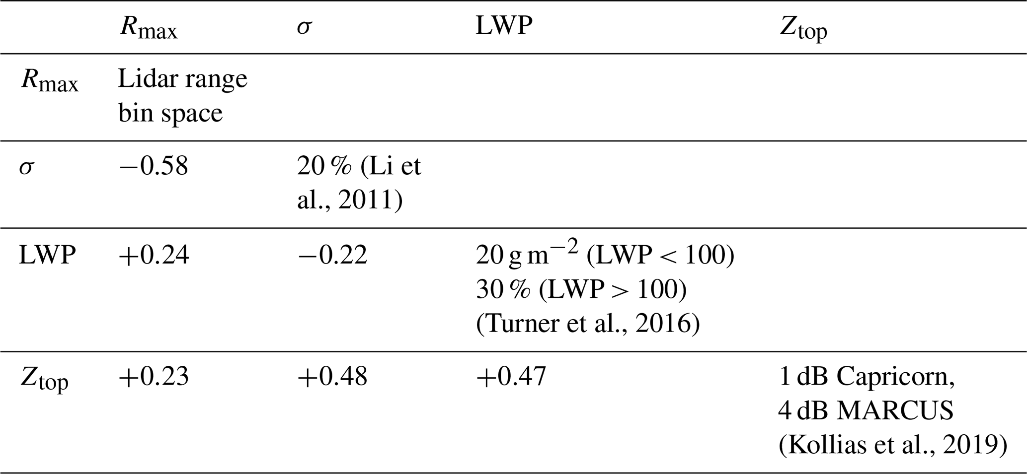
An observational error covariance matrix, S_y, is a 4 × 4 element matrix that records the uncertainty in the measurements in y due to random noise and uncertainties in the forward modeling of that quantity along the diagonal. We allow covariance among the observations using the correlations listed in Table 1 and the variances of the individual quantities as listed along the diagonal. These correlations are derived from the CAPRICORN II and MARCUS combined data set. We find significant correlations among the measurements in y. These correlations show that the measurements in y are not independent and are not, therefore, unique in terms of information. We address the information content below.

Table 1 Sources of uncertainty estimates (diagonal) and correlations (off diagonal) among measurements in y (Eq. 11) used in the OE algorithm. Correlations are derived from the combined MARCUS and CAPRICORN II data sets.

The quantities to be estimated and their covariance are denoted in the state vector x, respectively:

$$\begin{array}{}\text{(20)}& \mathit{x}=\left[\begin{array}{cc}{N}_{\mathrm{d}}& r_{\mathrm{e}}\end{array}\right].\end{array}$$

And S_x is a 2 × 2 element matrix that records the uncertainties in x along the diagonal. r_e is assumed to be near the layer top, as defined in Eq. (18).

We use x and additional observations and assumptions to derive a forward calculation of y or F(x) based on initial and incremental x guesses (see below) with a simple forward model. Our forward model begins with the observed thermodynamics such as temperature, pressure and relative humidity profiles, cloud base height, and layer thickness. With an observed or simulated LWP and a temperature-dependent Γ_l, we create a vertical profile of liquid water that varies with an adiabatic shape scaled by f_ad. Using an assumed shape parameter (α=2; justified below), we then calculate profiles of r_e and N_d, allowing us to estimate the terms in y, using the simple lidar equation (Eq. 10), and the expressions for Z and σ in Eqs. (6) and (5).

To derive x from y using OE, we express the first-order derivatives of y with respect to x in a Jacobian matrix, K_x, that has the dimensions of the number of elements in y (Eq. 19) by the number of elements in x (Eq. 20):

$${\mathbf{K}}_x=\begin{array}{llll}\frac{\partial R_{max}}{\partial N_{\mathrm{d}}}=-\mathrm{0.29}& \frac{\partial \mathit{\sigma }}{\partial N_{\mathrm{d}}}=\mathrm{0.24}& \frac{\partial \mathrm{LWP}}{\partial N_{\mathrm{d}}}=\mathrm{0}& \frac{\partial Z_{\mathrm{top}}}{\partial N_{\mathrm{d}}}=\mathrm{0.01},\\ \frac{\partial R_{max}}{\partial r_{\mathrm{e}}}=\mathrm{0.92}& \frac{\partial \mathit{\sigma }}{\partial r_{\mathrm{e}}}=-\mathrm{2.9}& \frac{\partial \mathrm{LWP}}{\partial r_{\mathrm{e}}}=\mathrm{0.44}& \frac{\partial Z_{\mathrm{top}}}{\partial r_{\mathrm{e}}}=\mathrm{1.2}.\end{array}$$

These terms are calculated analytically using the expressions in Eqs. (2)–(10), (14), and (17). Also, we set $\frac{\partial \mathrm{LWP}}{\partial N_{\mathrm{d}}}=\mathrm{0}$ because we assume that the amount of water made available for condensation is the result of thermodynamics, while how that water is distributed into droplets depends more on the CCN that is available for the water to condense onto. The quantities listed in the K_x matrix show typical values of the terms for case 5 listed in Table 2​​​​​​​ below in terms of $\frac{\partial \ln \left(y\right)}{\partial \ln \left(x\right)}$. We find that r_e influences σ, LWP, and Z_top in predictable ways. For instance, the derivative is negative in the r_e–σ relationship. The sensitivities of the observations in y are much more sensitive to r_e than to N_d, illustrating the challenge of retrieving N_d with remote sensing observations, as discussed earlier.

The OE formalism derives x by balancing the uncertainties and information in the measurements with what is known about the statistical properties of x given the atmospheric state. The information from prior knowledge is contained in an a priori vector of statistical estimates of the quantities in x (Eq. 21) or x_a and their covariance, S_a. For the prior estimate of N_d, we reason that coincident cloud condensation nuclei (CCN) measurements provide an upper limit on the droplet number. These measurements were collected during MARCUS and CAPRICORN II and are available hourly when the wind direction was favorable by not contaminating aerosol inlets with ship exhaust (Humphries et al., 2021). These hourly CCN measurements, collected by a Droplet Measurement Technologies (DMT) CCN-100 at 0.2 % supersaturation, are simply multiplied by 0.8 to account for coalescence processes and are used in x_a. We found that the use of CCN, while a broad constraint and upper bound on N_d, was quite necessary for accurate convergence of the OE algorithm. The hourly standard deviation of the CCN is then used along the diagonal of S_a. When CCN are not available within the previous 6 h, we use averages of the surface-based CCN measurements for the latitudinal bands from 40–50, 50–60, and > 60° S (Humphries et al., 2023). For the prior value of r_e, we use the 0.8 × CCN, the LWP, and layer thickness in Eq. (10). For r_e, we use in situ aircraft data collected during the Southern Ocean Clouds, Radiation, Aerosol Transport Experimental Study (SOCRATES; McFarquhuar et al., 2021) that was conducted in the Southern Ocean region south of Hobart, Australia, during the austral summer of 2018 by the NSF/NCAR High-performance Instrumented Airborne Platform for Environmental Research (HIAPER) Gulfstream V (GV) aircraft. In this campaign, the GV completed 15 research flights. We combine the Cloud Droplet Probe (CDP; manufactured by DMT) and 2D-S (manufactured by SPEC Inc.) measurements into a single droplet size distribution (DSD) and use a moments minimization method (Zhao et al., 2011) to estimate Eq. (1) for each low-level cloud 1 s DSD. See Baumgardner et al. (2017) and Lawson et al. (2006) for discussions of the in situ droplet probes. W-band radar reflectivity is then calculated using Eq. (6). For a particular retrieval where we have a measured Z_top, the SOCRATES data set is searched for all instances where Z is within 1.5 dB of the measurement, and the prior r_e is then estimated from the mean of the in situ measurements. For the covariance among the quantities in S_a, we know from the analysis of in situ data that r_e and N_d are strongly correlated (G18) at a level of ∼ 0.7 among those terms.

The OE formalism also allows us to quantify the added uncertainty in our forward model calculations due to model parameters and assumptions (Maahn et al., 2020; Austin and Stephens, 2001) which we take to include α (droplet distribution function shape parameter), f_ad (the adiabaticity of the column), and η. We find that a value of α=2 with a standard deviation of 1.5 reasonably characterizes the in situ cloud data collected during SOCRATES. f_ad is estimated by taking the LWP and cloud thickness observations collected over the MARCUS and CAPRICORN II voyages and deriving a linear regression of f_ad in terms of LWP following Miller et al. (1998); to wit, $f_{\mathrm{ad}}=\mathrm{1}.-(\mathrm{0.002}\times \mathrm{LWP})$. With LWP (in g m⁻²), this equation returns f_ad = 0.6 for LWP = 200 g m⁻² and 0.5 for LWP = 250 g m⁻². The scatter in the LWP − f_ad observations suggests an uncertainty in this estimate of 0.15. η is derived from the depolarization lidar data following the method described in Hu et al. (2007). While the uncertainty in this quantity is difficult to assess, when examining the consistency of the estimates over periods of persistent cloud cover, we determined that an uncertainty of 30 % is reasonable. A term of the form ${\mathbf{K}}_{\mathrm{b}}{S}_{\mathrm{b}}{\mathbf{K}}_{\mathrm{b}}^T$ is added to the instrumental uncertainties, where K_b is a Jacobian matrix that contains the first derivatives of the measurements in y with respect to α, f_ad, and η determined through finite differences in the forward model:

$${\mathbf{K}}_{\mathrm{b}}=\begin{array}{lll}\frac{\partial R_{max}}{\partial \mathit{\alpha }}=-\mathrm{0.08}& \frac{\partial R_{max}}{\partial f_{\mathrm{ad}}}=-\mathrm{0.60}& \frac{\partial R_{max}}{\partial \mathit{\eta }}=-\mathrm{0.63},\\ \frac{\partial \mathit{\sigma }}{\partial \mathit{\alpha }}=\mathrm{0.11}& \frac{\partial \mathit{\sigma }}{\partial f_{\mathrm{ad}}}=\mathrm{0.55}& \frac{\partial \mathit{\sigma }}{\partial \mathit{\eta }}=\mathrm{0.03},\\ \frac{\partial \mathrm{LWP}}{\partial \mathit{\alpha }}=\mathrm{0.20}& \frac{\partial \mathrm{LWP}}{\partial f_{\mathrm{ad}}}=\mathrm{1.0}& \frac{\partial \mathrm{LWP}}{\partial \mathit{\eta }}=\mathrm{0.0},\\ \frac{\partial Z_{\mathrm{top}}}{\partial \mathit{\alpha }}=-\mathrm{0.35}& \frac{\partial Z_{\mathrm{top}}}{\partial f_{\mathrm{ad}}}=\mathrm{2.0}& \frac{\partial Z_{\mathrm{top}}}{\partial \mathit{\eta }}=\mathrm{0.0}.\end{array}$$

The numbers in the K_b matrix expression are in terms of $\frac{\partial \ln \left(y\right)}{\partial \ln \left(x\right)}$ and are derived from the forward model over the physically reasonable ranges of the parameters. We find that these numbers vary by less than 20 % in the Capricorn and MARCUS data sets. S_b contains the variance of α, f_ad, and η determined from in situ and remote sensing measurements. We assume that the covariance among these quantities can be neglected.

The inversion of y for x then follows a standard iterative approach by applying a Gauss–Newton minimization technique derived in Rodgers (2000); see also Maahn et al. (2020). In this approach, successive guesses of x are derived using the well-known expression,

$$\begin{array}{}\text{(21)}& \begin{array}{rl}\mathit{\delta }x=& {\left(S_{\mathrm{a}}+{\mathbf{K}}_x{\mathbf{S}}_y{\mathbf{K}}_x^T\right)}^{-\mathrm{1}}\left[{\mathbf{S}}_{\mathrm{a}}^{-\mathrm{1}}\left(\widehat{x}-x_{\mathrm{a}}\right)\right.\\ & \left.+{\mathbf{K}}_x^T{\mathbf{S}}_y^{-\mathrm{1}}\left(y-F\left(\widehat{x}\right)\right)\right],\end{array}\end{array}$$

where $\widehat{x}$ is a present guess, $F\left(\widehat{x}\right)$ is the forward estimate of the measurements in y using the present guess. δx then becomes the next increment on $\widehat{x}$. Equation (21) is iterated until either a convergence criterion is met or divergence of the result occurs. Typically, fewer than 10 iterations are necessary if the algorithm converges, which it does > 90 % of the time in non-precipitating conditions, while convergence occurs less frequently as drizzle and light snow increase due to the inability to accurately estimate R_max.

2.5 Optimal estimation algorithm evaluation

The response of the OE algorithm is equivalent to the results presented in Fig. 3, except that additional information is used to hopefully lessen the effects of uncertainty in R_max. In Table 2, we list six cases that we use to examine the response of the OE algorithm in terms of the retrieved quantities and their uncertainties. Cases 2, 4, and 6 differ from cases 1, 3, and 5, respectively, only by the level of uncertainty applied. Cases 2, 4, and 6 use 2 times the listed uncertainties in cases 1, 3, and 5, but otherwise have identical inputs. Cases 1 and 2 are designed to illustrate a situation that might be found in a heavy aerosol environment with a low R_max, high σ, and low Z_top that produces high N_d, small cloud drops, and moderately high LWP. Cases 3 and 4 show the opposite with a rather large R_max and lower σ. Z_top is set higher with a larger LWP. The algorithm returns a small N_d and large r_e in cases 3 and 4. Cases 5 and 6 are in between the two extremes. f_ad in these cases range from 0.8 to 0.9, and this is by design, as the cloud depth is specified. The uncertainties listed in Table 2 are used in cases 1, 3, and 5; except for Z_top, which is listed in decibels, the uncertainties are a fraction of the measurement. As a fraction of the returned values, the 1 standard deviation uncertainties do not change significantly from case to case, and they respond predictably to a doubling of the observational errors that increase approximately by a factor of 2. We also test the OE uncertainty by randomly perturbing the observations about their stated uncertainties until the error statistics converge. These are reported in Table 2 in the “bootstrapping” rows. The bootstrap experiment generally returns uncertainty in r_e that is equivalent to or slightly smaller than the OE results. For N_d, the bootstrap experiment returns marginally larger uncertainties than the OE results.

Table 2 Cases used to illustrate the response of the OE algorithm. Observables are listed in columns 2–5 with uncertainties in parentheses. The retrieved quantities, their uncertainties in the OE algorithm, and using a bootstrap approach (see text) are in lower rows. We also list the Shannon information content in bits and the number of independent observations in the retrieval as derived from the OE formalism; see Rodgers (2000). Cases 2, 4, and 6 have observational uncertainties that are a factor of 2 greater than cases 1, 3, and 5.

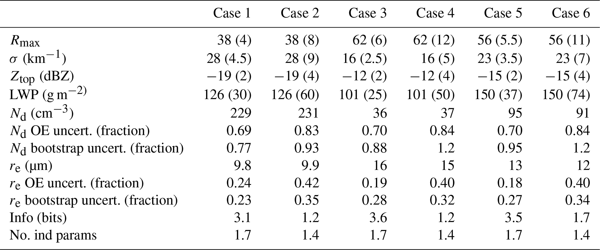
The Shannon information content measures the extent to which the observations reduce the uncertainty in the prior. The studies of L'Ecuyer et al. (2006) and Cooper et al. (2006) provide detailed discussions of this concept. Doubling the observational uncertainty reduces the information content by approximately one-third. The number of independent parameters is fewer than the number of elements in y (the observations) because the observations are correlated. For instance, as shown in Table 2, R_max and σ both constrain N_d, while LWP and Z_top constrain r_e. Even in the lower error cases, the observations do not provide sufficient information to retrieve three independent quantities, suggesting that the results are correlated and not independent.

The uncertainty in r_e remains roughly equivalent to the results shown in Fig. 3, although we consider the results of the OE to be more accurate because a better accounting of the information is used. Notable is the magnitude of the uncertainties for the retrieved N_d. We find that it remains large, although the additional information provided by the other observations reduces the uncertainty compared to the results in Fig. 3. We also tested how well the OE algorithm without R_max would do where just extinction is the primary constraint on N_d. This was accomplished by setting the K_x term as $\frac{\partial R_{max}}{\partial N_{\mathrm{d}}}=\mathrm{0}$. We found that for the uncertainties in the other quantities listed in Table 2, the uncertainty in N_d was approximately 150 %, showing that R_max is a useful quantity in this regard. However, retrieval of N_d remains highly uncertain when the lidar range bin spacing exceeds 5 m.

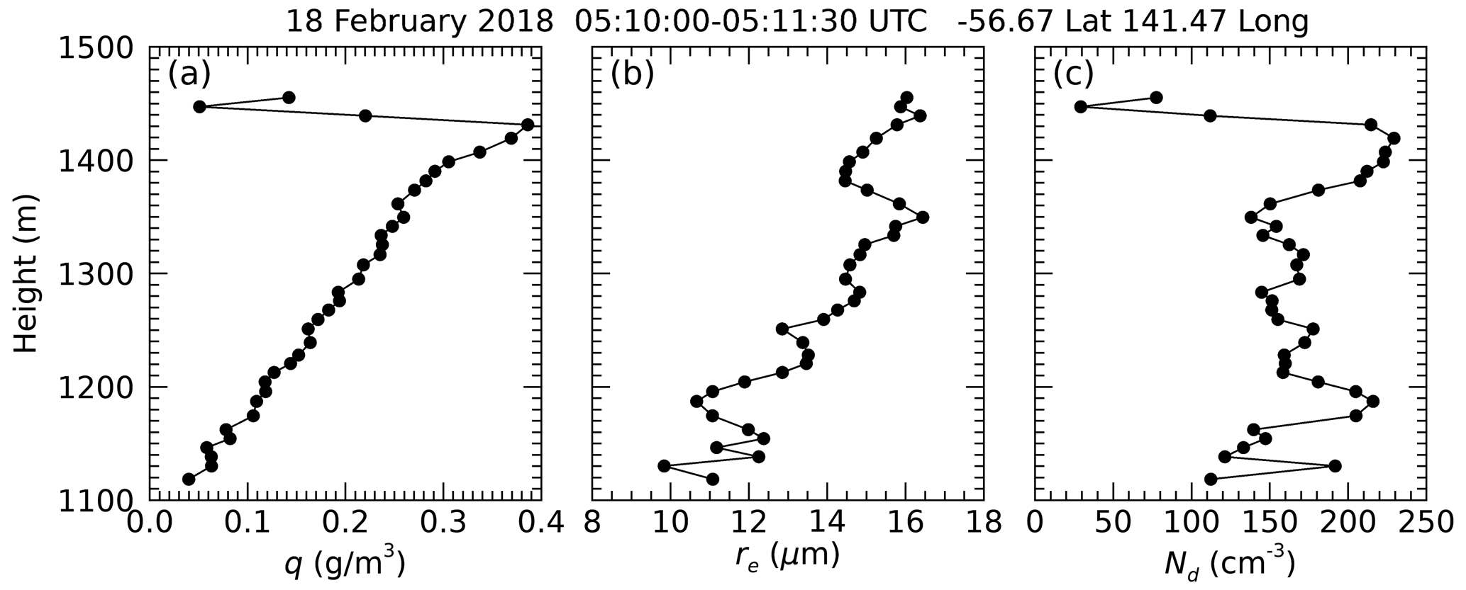
Figure 4 Ramp through a marine boundary layer (MBL) cloud layer on 18 February 2018 collected by instruments on the NSF/NCAR Gulfstream V during SOCRATES. This ramp was conducted near R/V Investigator during CAPRICORN II. As a function of height between the cloud base near 1100 m and cloud top near 1450 m, the panels show (a) q, (b) r_e, and (c) N_d.

To provide a more realistic evaluation of the OE algorithm performance, we use data collected during the SOCRATES campaign, where ramps (constant rate ascents and descents between cloud base and cloud top) through low-level cloud layers were conducted. Such a ramp is depicted in Fig. 4 which was collected on 18 February 2018 (hereafter 2/18) at 05:10 UTC when the GV was conducting a mission near R/V Investigator at 57° S and 142° E. We will expand on the 18 February case study below. For this analysis, we focused on 1 s data collected by the CDP that recorded droplet spectra in 2 µm size bins up to 50 µm. The aircraft entered the cloud layer with a temperature near −5 °C at 1100 m. q and r_e steadily increased as the GV ascended and exited the cloud layer approximately 90 s later at an altitude of 1450 m, where q reached a maximum of 0.4 g m⁻³ and was ∼ 15 µm near the cloud top. We note an interesting structure in the vertical r_e profile, with a sudden decrease near 1375 m. During this ascent, N_d was quite variable but averaged 150 cm⁻³ through most of the ramp until 1375 m where there is an abrupt increase in N_d to ∼ 225 cm⁻³ in conjunction with the decrease in r_e. Integrating q vertically through the layer, the LWP was 65 g m⁻², with an adiabatic LWP of 80 g m⁻², suggesting a sub-adiabatic layer with f_ad of ∼ 0.8. The radar reflectivity time series (discussed later) shows that drizzle was occurring sporadically during this case. We used the cloud droplet concentrations collected during the ramp to get R_max (32 m), the expression for Z (Eq. 6) to estimate Z_top (−15 dBZe), and the cross-sectional area of the droplet distribution to estimate σ (layer mean of 30 km⁻¹ and layer optical depth (τ) of 14). These values were used as input to the lidar forward model. We implement the OE algorithm with f_ad and LWP to get a retrieved N_d of 165 cm⁻³ and r_e of 14 µm, which is in reasonable agreement with the input data.

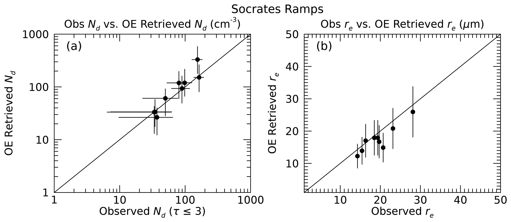
Figure 5 Comparison of observed and derived N_d (a) and r_e (b) from SOCRATES ramps. The error bars on the retrieved quantities are as derived from the optimal estimation.

We repeated this exercise for other ramps collected during SOCRATES, excluding ramps that were super-adiabatic or had non-adiabatic structure in the vertical profile, reasoning that the finite distance over which the ramps occurred (∼ 10–20 km) had the potential to sample cloud elements of varying properties. For instance, on 2/18, three additional ramps were rejected. The observational uncertainties used in the inversion are as discussed above for cases 1, 3, and 5. Figure 5 shows the relationship between the observed and retrieved N_d and r_e, showing that the OE algorithm can reasonably capture the characteristics of the cloud layers. While we would expect the algorithm to provide a reasonable comparison of the retrieved and observed N_d and r_e in this rather contrived experiment, we note that the OE uncertainty, for the most part, extends over the 1 : 1 line, suggesting that the characterization of uncertainty in the retrieved quantities is a reasonable estimation of the actual uncertainty in the algorithm.

3 Results and discussion

In this section, we present independent comparisons of the results of the N_d OE algorithm using a detailed case study collected when the Terra satellite passed over R/V Investigator approximately 1 h prior to an in situ sampling period conducted by the NSF/NCAR GV during SOCRATES on 18 February 2018 (2/18). We then expand our view to examine comparisons of multiple overpasses of the ship by the NASA MODIS instrument on the Terra and Aqua satellites during the 2018 summer campaigns.

3.1 A case study

The 2/18 case study provides a unique opportunity for independent comparisons of the algorithm with data collected while the GV aircraft operated in the vicinity of R/V Investigator and with an overpass of the Terra satellite that provided independent retrievals of τ and r_e (Platnick et al., 2003) from which we can derive LWP and N_d (G18) using the MODIS τ and r_e. During this case study period, the ship remained stationary at 56.6° S and 141.5° E to facilitate coordination with the GV. Figure 6 illustrates the data collected from the shipboard instruments. The lidar-attenuated backscatter indicates a fully attenuating layer through the entire period. With a cloud base temperature near −5 °C, the lidar depolarization ratio data suggest that the cloud base phase and the subcloud precipitation were liquid. The W-band radar on R/V Investigator indicated episodic drizzle events of 10–20 min duration roughly every hour, and some of it was rather heavy. Intervening periods without drizzle had radar reflectivity near the detection threshold of the radar (∼ −25 dBZe in the CAPRICORN II configuration). The radar and sounding data collected at the ship showed that the layer was topped by a strong marine inversion near 1.5 km, which is in agreement with the GV ramp in Fig. 4. The LWP was variable between 50–60 g m⁻² during periods without drizzle to values near 250 g m⁻² during periods of drizzle. The retrieved cloud properties varied depending on the proximity of a drizzle event. While the algorithm did not converge in regions of heavier drizzle, we find near the boundaries of several drizzle events that the N_d decreased to 20–30 cm⁻³ and r_e increased to be more than 20 µm. Otherwise, the algorithm tended to produce N_d in the range of 100 cm⁻³ and r_e in the 10 µm range.

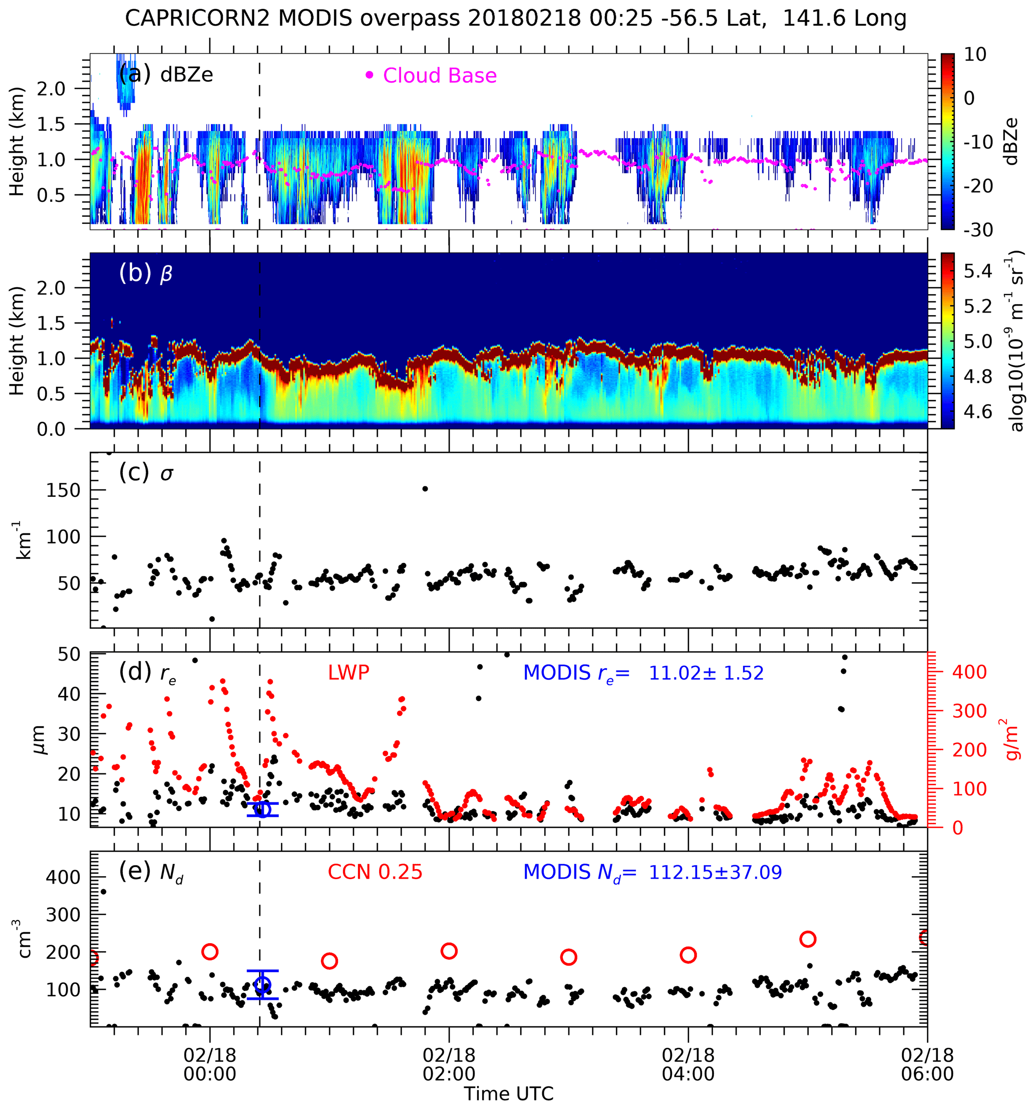
Figure 6 Surface-based measurements and derived properties from data collected on 18 February 2018 on R/V Investigator near 55.6° S and 141.5° E. (a) Radar reflectivity (Z) with the ceilometer cloud base indicated by purple dots, (b) lidar-attenuated backscatter, β_obs, (c) extinction derived from β_obs, (d) r_e and LWP, and (e) N_d. The blue circles in panels (d) and (e) and the inset values are from an overpass at 00:25 UTC (vertical dashed line) of MODIS on Terra. CCN at 0.25 % supersaturation is shown in panel (e) using red circles.

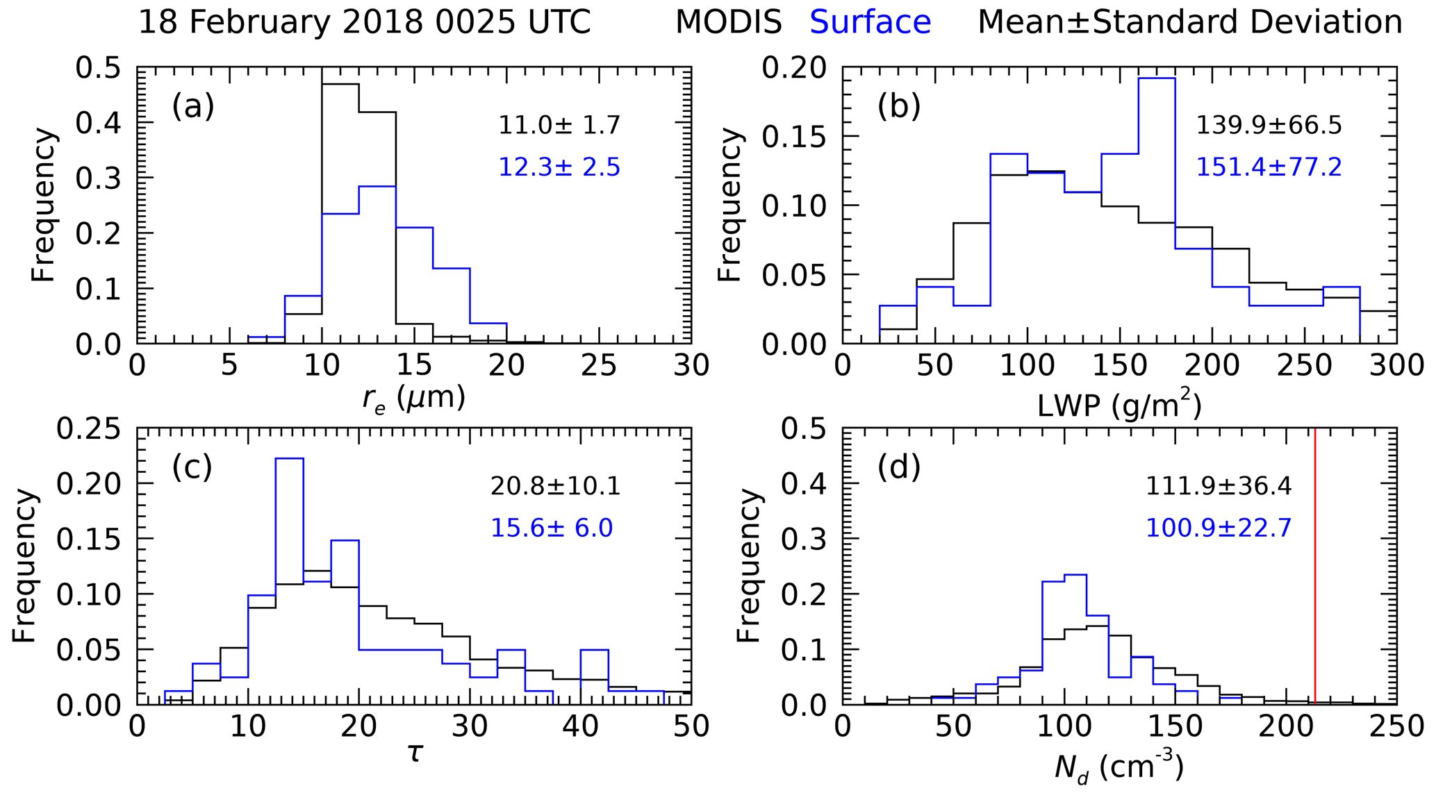
Figure 7 Comparison of properties observed and derived from data collected on R/V Investigator (blue) with cloud properties derived from a Terra MODIS overpass at 00:25 UTC on 18 February 2018. (a) r_e, (b) LWP, (c) optical depth, and (d) N_d. The vertical red line in panel (d) shows the 0.25 % supersaturation CCN measured on R/V Investigator at this time.

A Terra MODIS overpass occurred at 00:25 UTC. We collect the level 2 retrieval of τ and r_e in a region of 50 km diameter centered on the ship, and the ship data are collected between 23:00 UTC on 17 February and 01:30 UTC on 2/18. The comparison results are shown in Fig. 7 (see also Fig. 6). A broad distribution of LWP is demonstrated during this period that has a similar character in both data sets. The ship has an LWP mode near 160 g m⁻² that is due to the drizzle event that is evident near 00:00 UTC in Fig. 6. The mean LWP from the ship is slightly larger than MODIS, but the two are in broad agreement. The distributions of r_e in the two data sets overlap with the surface data skewed to larger values, likely because of the predominance of the drizzle event. The N_d retrievals also demonstrate broad agreement with quite wide distributions, even though the ship N_d is skewed to smaller values. The ship τ distribution is skewed to smaller values than MODIS, consistent with larger r_e and smaller N_d. We note that τ and r_e are the quantities that are most directly retrieved from the MODIS algorithm, whereas the LWP and especially N_d require additional assumptions.

On the other hand, the surface data LWP is independent of the radar, lidar, and other measurements and requires a minimum of assumptions to derive from the microwave radiometer brightness temperatures (Turner et al., 2016). N_d and r_e from the surface data require a complicated algorithm, and τ from the surface data is calculated using Eq. (9). Thus, the surface-derived τ would include the errors in the surface retrieval of r_e. While there are biases in the comparison, given the substantial differences in the two independent data sets, we conclude that the comparisons demonstrate a reasonably consistent picture of the cloud field during the overpass.

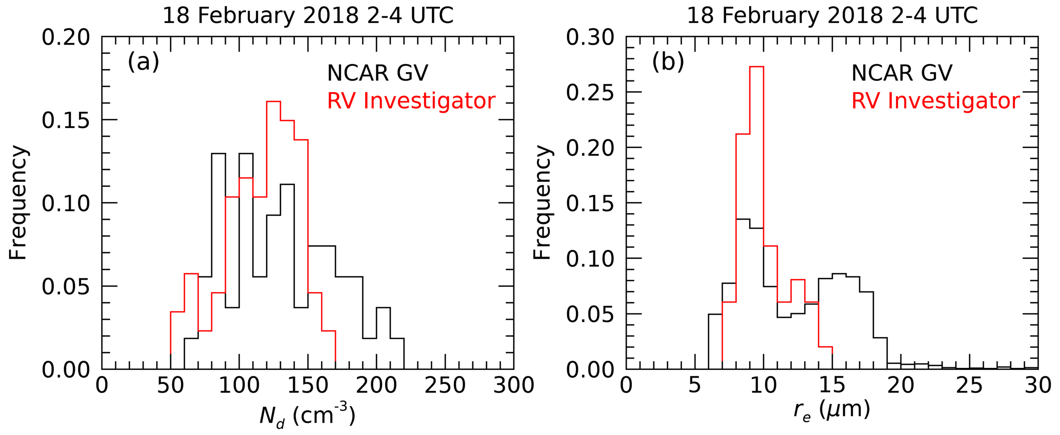
Figure 8 Comparison of N_d (a) and r_e (b) derived from the surface-based data collected on R/V Investigator (red) with data collected from the NSF/NCAR GV on 18 February 2018. Cloud properties are compiled over the period from 02:00–04:00 UTC.

The GV arrived at the ship at approximately 02:00 UTC on 2/18 and operated in the vicinity of the ship for roughly 2 h. It conducted ramps, level legs within the cloud layer, and legs above and below the layer for aerosol and remote sensing applications. We compare data collected during this time by gathering the aircraft data within 50 km of the ship. The effective radius is derived from the aircraft CDP data in the upper half of the layer (above 1.2 km), and the aircraft N_d is collected from the CDP data in the lowest half of the layer. The comparison of N_d and r_e distributions is shown in Fig. 8. The aircraft r_e data are bimodal, while the ship retrieved r_e are unimodal and centered on the lower mode of the aircraft r_e distribution. We interpret the lack of bimodality in the ship-based r_e data as being due to the algorithm not converging in regions of heavier drizzle as noted above. The aircraft penetrations of drizzle and non-precipitating clouds result in the bimodality in the r_e distribution, as shown in Fig. 8. The N_d distributions are broadly similar, but the ship results are biased to lower values. The extent to which there is a bias toward the lower part of the cloud layer in the ship data is unclear. Regardless, both distributions are centered just in excess of 100 cm⁻³. This comparison suggests that the surface-based OE algorithm reasonably replicates the cloud layer properties in this case.

Overall, we find that the aircraft, satellite, and surface-based data sources provide similar and very interesting characterizations of the cloud and CCN on 2/18. Twohy et al. (2021) in their Supplement show that the air mass above the marine boundary layer on 2/18 had one of the highest sulfur-based concentrations of CCN recorded during SOCRATES at 224 cm⁻³. The air mass observed on 2/18 followed a trajectory from the deep south over the Antarctic continent and the biologically productive waters of the Southern Ocean. The high concentrations of sulfate CCN in the free troposphere imply that the new particle formation along the trajectory was likely responsible for the high CCN (McCoy et al., 2021). The CCN at the surface measured on R/V Investigator was near 210 cm⁻³, which is slightly lower than that measured on the aircraft.

On the other hand, N_d seems to be consistently in the 100 cm⁻³ range from the surface, ship, and MODIS, except for the near-cloud-top maxima in N_d observed by the GV in the ramp demonstrated in Fig. 4. The other ramps (not shown) also had values of N_d near the CCN values of 200–250 cm⁻³. We speculate that the difference between CCN and N_d is mostly likely due to precipitation droplet scavenging and coalescence process that is actively generating drizzle in this case. The high CCN from the free troposphere transported to this location from the south is likely mixing into the marine boundary layer through entrainment (the cloud-top spike in N_d in Fig. 4) and being processed through clouds explaining the lower surface CCN. The cloud properties (N_d in the 100 cm⁻³ range) are a drizzle- and coalescence-damped response to the higher free-tropospheric CCN.

3.2 Expanded MODIS comparison

Finally, we compare with the MODIS-derived cloud properties from overpasses of the ships during the MARCUS and Capricorn campaigns. With MODIS instruments on the Terra and Aqua satellites and the ships being at sea over extended periods, we found several events where suitable low-level clouds occurred over the ships during MODIS overpasses. Table 3 lists the information about the 14 overpasses of the ships that we use for the comparison in Fig. 9. Our approach was to examine a 50 km region of MODIS data centered on the ship, and we compiled surface data from 90 min periods before and after an overpass. We find reasonable agreement in the comparisons. The LWP is an interesting quantity since, as stated above, it is independent of the N_d−r_e retrieval. The LWP from the MODIS data, on the other hand, is derived from the τ and r_e algorithm that uses a bispectral method (Nakajima and King, 1990) so that the MODIS LWP would carry forward any uncertainties in τ and r_e. The agreement, however, is reasonable and with little bias. Most of the cases have LWP < 200 g m⁻², since we focus on non- to lightly precipitating cloud scenes. The r_e of the cases range over values that are very small, corresponding to cases near the Antarctic continent with high N_d and no precipitation to r_e that exceeds 15 µm. The comparison in r_e is unbiased and with a reasonable correlation. While N_d also demonstrates a reasonable correlation, there does appear to be a slight bias in the comparison, with the surface data being, on average, 20–30 cm⁻³ higher than MODIS. The optical depth appears unbiased for values smaller than ∼ 15 but then seems to show a bias for values of more than 15, with MODIS being larger than the surface-based results. More data are highly desirable to establish how well and under what circumstances these data sets agree or not, but this comparison is encouraging.

Table 3 List of the MODIS overpasses shown in Fig. 9.List of the MODIS overpasses shown in Fig. 9.List of the MODIS overpasses shown in Fig. 9.List of the MODIS overpasses shown in Fig. 9.List of the MODIS overpasses shown in Fig. 9.

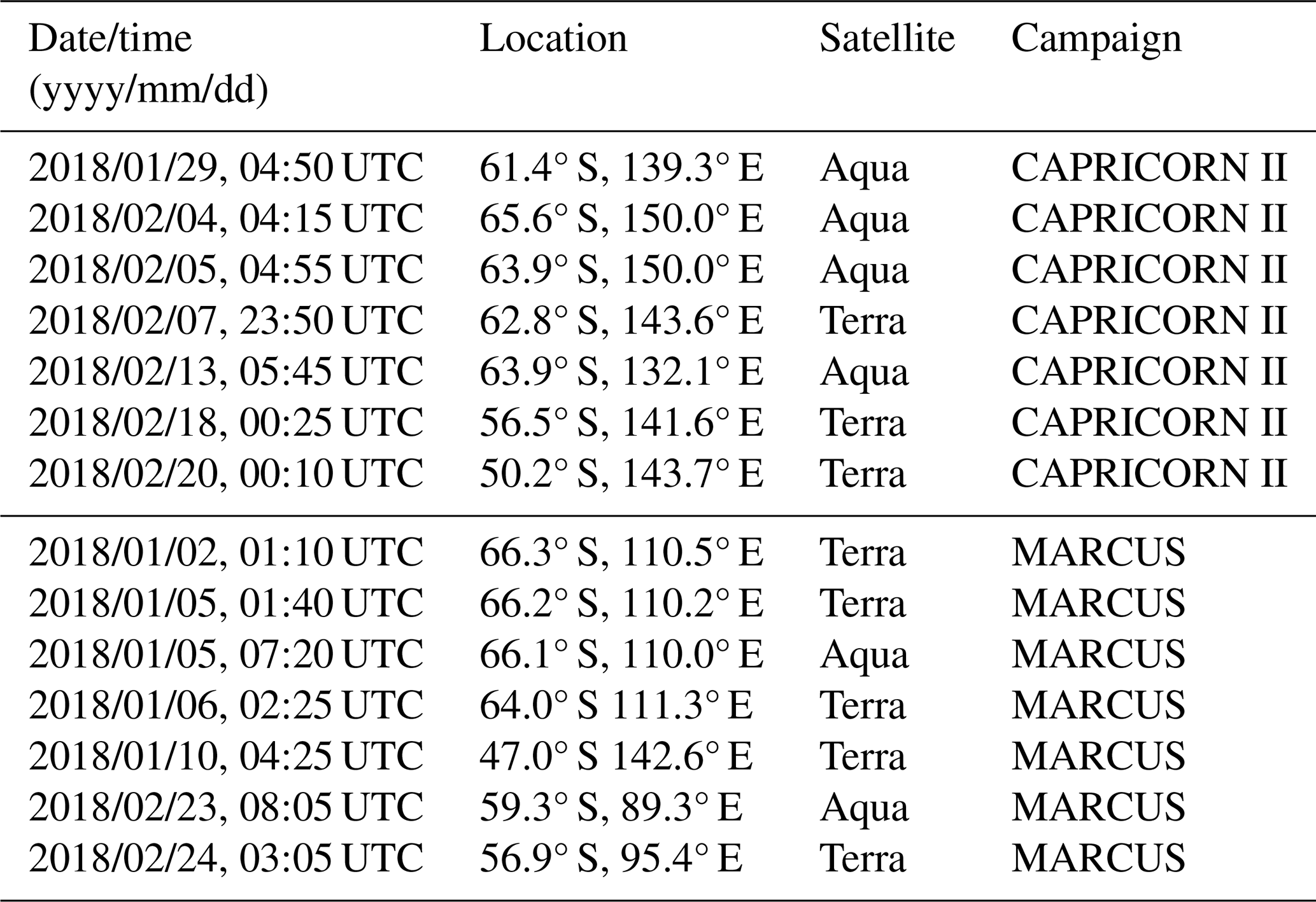
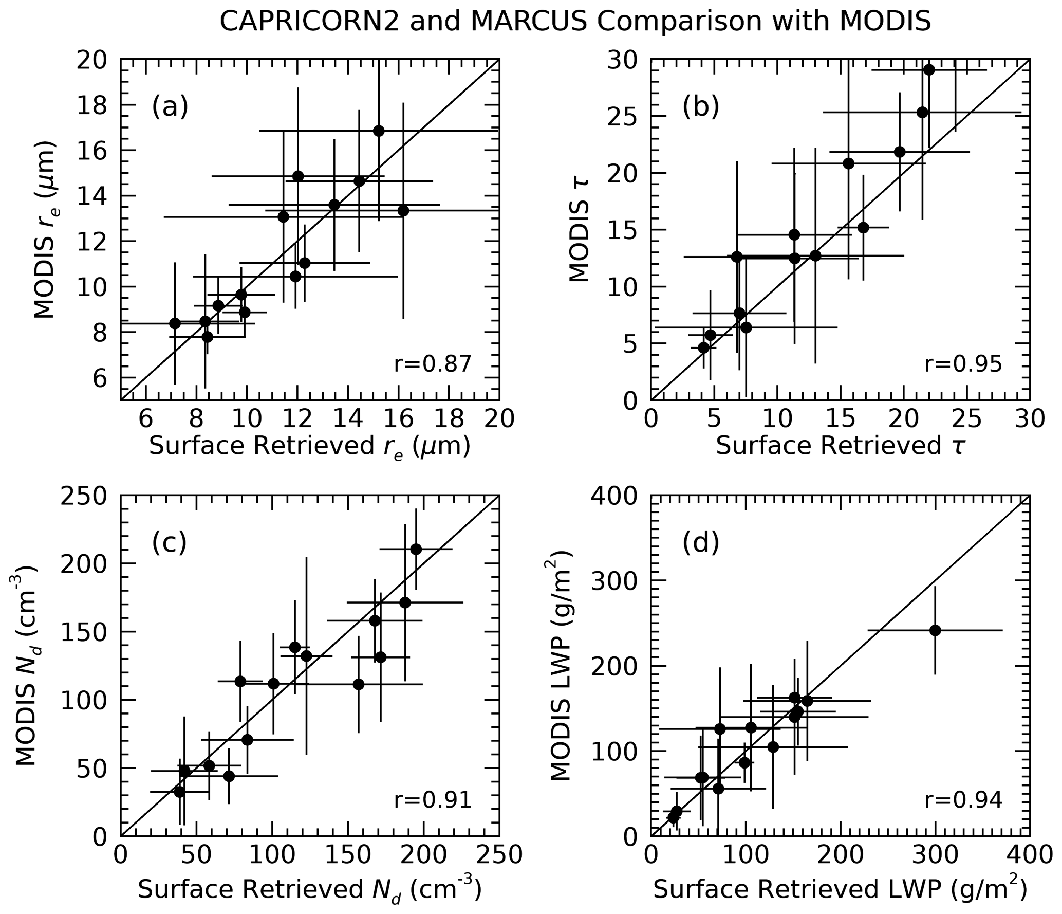
Figure 9 Comparison of MODIS-derived cloud properties with cloud properties derived from data collected during the MARCUS and CAPRICORN II campaigns in the Southern Ocean during austral summer 2018. Error bars are 1 standard deviation of the retrieved cloud properties during the time and over the spatial extent of the two data sets. The Pearson correlation coefficient of the comparison is shown as an inset in each panel.

4 Summary and conclusions

Given the importance of knowing cloud droplet number concentrations (N_d) in low-level clouds for understanding how these clouds interact with aerosol and precipitation-producing processes to influence the Earth's albedo, we have explored two techniques that allow us to derive N_d and layer effective radius (r_e) using surface-based remote sensing techniques with an emphasis on the information brought to this problem by lidar data. The depth that a laser pulse penetrates a cloud layer is a function of the amount of water droplet cross-sectional area presented to the laser pulse, and that cross-sectional area is dependent upon the N_d and the liquid water content (q). This observable is quantified by the lidar-attenuated backscatter, β_obs (Eq. 10), that is modulated by the directionality of the scattering as represented by the multiple scattering factor. As the lidar beam penetrates a cloud layer, the signal initially increases until two-way attenuation causes the signal to reach a maximum, after which it decays exponentially, depending upon multiple scattering. The rate of increase in β_obs is easily quantified if N_d and q are known or, turning the problem around, one can calculate N_d if β_obsis observed and q is known. The math becomes more tractable where the lidar signal is at a maximum (a distance we term R_max), since the rate of change in β_obs is zero there (Eqs. 16 and 17). The liquid water content, q, can be expressed in terms of the rate of increase in q with height for an adiabatic cloud, which can be made more realistic by scaling the q profile by an adiabaticity factor that can be derived from LWP and cloud layer depth. This simple model (Eq. 17) can be implemented with an estimated cloud depth, LWP, and a lidar. The effective radius near the cloud top can then be derived (Eq. 18).

The method, however, is very sensitive to uncertainty in R_max which is, in turn, dependent on the vertical resolution of the lidar. Since R_max typically ranges from a few tens of meters to maybe as much as 100 m, the uncertainty in derived N_d becomes prohibitively large (> 100 %) for range resolutions much above 15 m. R_max also depends on an estimate of where in the vertical profile activation of cloud droplets begin. In non-precipitating clouds, this level is easily discerned to be where the signal first rises significantly above the aerosol and molecular background. In light precipitation, this level is less obvious, and we extrapolate the signal to a level of signal strength that was previously identified in non-precipitating conditions. We found empirically that the cloud base identified by most automated ceilometer or lidar algorithms typically identify a cloud base to be very near where the lidar-attenuated backscatter reaches a maximum which is not useful in this context. Uncertainty in R_max translates predictably into uncertainties in r_e. Another limitation of the method is the need to estimate the q profile above cloud base. We take advantage of an assumed adiabatically shaped q profile to estimate q at the point where β_obs reaches a maximum. This allows us to essentially have two pieces of information to solve Eq. (2), with the third, α, being assumed. A cloud that does not have this adiabatic shape in q would, therefore, not provide an accurate estimate of N_d and r_e. Additionally, the cloud must be fully attenuating to have an accurate value for R_max. We assume that most optically thick stratocumulus would satisfy these assumptions. Note that it would be difficult to adapt this method to down-looking observing systems from aircraft or satellite because of the assumption of the adiabatic shape of the q profile. The tops of many marine boundary layer (MBL) clouds contain a region where q is decreasing with height from a layer of maximum q due to the interaction with dry air at the layer top. The depth of this region would depend on the strength of the marine inversion and the amount of mixing.

To lessen the effects of uncertainty in R_max, we bring more information to bear on the problem by quantifying the cloud layer extinction in terms of the rate of decay of the lidar signal beyond R_max using a published methodology (Li et al., 2011). In addition, we use the radar reflectivity near the cloud top as a constraint on the q profile and r_e. This is cast in an optimal estimation (OE) algorithm that seeks to balance the uncertainty in the observations and uses prior information such as CCN concentrations that provide an upper limit on N_d. The OE algorithm is only marginally successful in reducing the uncertainty in N_d and r_e. The uncertainties, especially on N_d, remain substantial since R_max provides the most significant information on N_d, and the other measurements provide minimal constraint on N_d, as quantified in the Jacobian (K_x) matrix. What we find interesting but not surprising is that the use of CCN as a prior constraint allows us to balance the information content in R_max and the other observations with what we know as a significant constraint on N_d and, to a lesser extent, r_e. Overall, the OE uncertainties that are shown to be reasonable through a bootstrapping experiment and through comparison to aircraft data are in the range of just under a factor of 2 for N_d and 30 % for r_e for lidar range bins of 10–30 m. The only way to reduce this uncertainty is to have dedicated lidar measurements that have a vertical resolution that is smaller than 10 m. Using comparisons with in situ aircraft data and with cloud properties derived from MODIS, we show that the OE algorithm provides results consistent with the uncertainty in the data and retrievals.

Finally, a case study is explored that shows how synergistic remote sensing data from the surface, especially when combined with aircraft and satellite data, can be exploited. The 18 February 2018 case study that took place in the Southern Ocean near 56° S and 141° E suggests how long-range aerosol transport of an air mass from the biologically productive waters of the deep southern latitudes modulated the cloud properties that existed on this day. The CCN measured at the surface and from the GV aircraft was about a factor of 2 larger than the ∼ 100 cm⁻³ N_d inferred from the ship-based remote sensing and MODIS data and observed by the GV. This difference between N_d and CCN was likely a response to the widespread precipitation processes that were occurring on this day.