Scale separation for gravity wave analysis from 3D temperature observations in the mesosphere and lower thermosphere (MLT) region

MATS (Mesospheric Airglow/Aerosol Tomography and Spectroscopy) is a Swedish satellite designed to investigate atmospheric dynamics in the mesosphere and lower thermosphere (MLT). By observing structures in noctilucent clouds over polar regions and oxygen atmospheric-band (A-band) emissions globally, MATS will provide the research community with properties of the MLT atmospheric wave field. Individual A-band images taken by MATS's main instrument, a six-channel limb imager, are transformed through tomography and spectroscopy into three-dimensional temperature fields, within which the wave structures are embedded. To identify wave properties, particularly the gravity wave momentum flux, from the temperature field, smaller-scale perturbations (associated with the targeted waves) must be separated from large-scale background variations using a method of scale separation. This paper investigates the possibilities of employing a simple method based on smoothing polynomials to separate the smaller and larger scales. Using using synthetic tomography data based on the HIAMCM (HIgh Altitude Mechanistic general Circulation Model), we demonstrate that smoothing polynomials can be applied to MLT temperatures to obtain fields corresponding to global-scale separation at zonal wavenumber 18. The simplicity of the method makes it a promising candidate for studying wave dynamics in MATS temperature fields.

1 Introduction

Gravity waves (GWs) are important features of the dynamics of the Earth's atmosphere. They can be generated through numerous mechanisms, e.g. flow over topography, convection, and geostrophic adjustment processes (Fritts and Alexander, 2003). GWs may propagate over long distances from their sites of generation, redistributing energy and momentum geographically as well as vertically. As the waves break, these dynamical quantities are transferred to the surrounding medium, affecting its temperature and motion. On a global scale, the redistribution of energy and momentum due to GWs affects circulation patterns in the middle atmosphere, generating pole-to-pole circulation in the mesosphere (Lindzen, 1981; Holton, 1982). Through their body forces, breaking waves may generate secondary waves, which may, in turn, generate tertiary waves (Vadas and Fritts, 2002; Vadas and Becker, 2019). As the waves perturb density, pressure, and temperature, their presence leaves structures in noctilucent clouds (Pautet et al., 2011; Taylor et al., 2011) and atmospheric airglow (Nakamura et al., 1999; Medeiros et al., 2004).

MATS (Mesospheric Airglow/Aerosol Tomography and Spectroscopy) is a Swedish satellite funded by the Swedish National Space Agency (Gumbel et al., 2020). MATS was launched on 4 November 2022 from Te Māhia / Māhia Peninsula, New Zealand, with the scientific objective of identifying and quantifying atmospheric wave activity in the mesosphere and lower thermosphere (MLT). To accomplish its mission, MATS carries a six-channel limb imager with two main IR channels centred on 762 and 763 nm, targeting airglow emissions in the ${\mathrm{O}}_{\mathrm{2}}{(}^{\mathrm{1}}{\mathrm{\Sigma }}_g^{+}{-}^{\mathrm{3}}{\mathrm{\Sigma }}_g^{-})$ atmospheric band (“A band”). The channels produce 2D images of the atmospheric limb. Through tomography and spectroscopy, individual images taken along the orbit track are combined to produce three-dimensional temperature fields (Gumbel et al., 2020). From these 3D fields, gravity wave properties will be derived, including global maps of wave vectors, wave amplitudes, and the vertical flux of horizontal gravity wave pseudomomentum.

The first step to identify wave properties from temperature measurements is to isolate the wave-induced disturbances T^′, as well as the corresponding background $\stackrel{\mathrm{‾}}{T}$, from the full temperature T. For this, a background removal scheme is applied to the data. Following linear wave theory, the temperature measurements made by MATS can be considered to consist of a superposition of the large-scale structures; the temperature background $\stackrel{\mathrm{‾}}{T}$; and the smaller-scale structures due to the GWs, i.e. the temperature residuals T^′, given as

$$\begin{array}{}\text{(1)}& T(x,y,z,t)=\stackrel{\mathrm{‾}}{T}(x,y,z,t)+T^{\prime }(x,y,z,t).\end{array}$$

The coordinates in Eq. (1) refer to the geometry of the MATS tomography output, where x refers to the along-track distance, y refers to the across-track distance, z refers to the height, and t refers to the time. Different methods for background removal have been discussed by Sakib and Yigit (2022). The separation of scales is typically based on research interests and/or measurement limitations. Ideally, all of the waves that are small enough to be identified in the MATS data geometry should be included in the residual field, and larger structures should be included in the temperature background.

The distinction between scales is typically made based on the zonal wavenumber (ZWN),

$$\begin{array}{}\text{(2)}& k={\displaystyle \frac{\mathrm{2}\mathit{\pi }R\cos \mathit{\phi }}{\mathit{\lambda }}},\end{array}$$

where R is the radius of the Earth, λ is the wavelength in the zonal direction, and φ is the latitude. One method of performing scale separation is fitting waves in the zonal direction and cutting at a specified zonal wavenumber. This method can be combined with polynomial smoothing in the meridional direction (Ern et al., 2018; Strube et al., 2020). Low wavenumbers are associated with the background, and high wavenumbers are associated with the GW fields. This method has the advantages of a clear cut in the horizontal wave spectrum and no degradation in the vertical wave spectrum of the temperature residuals. It is easily performed on model data on synoptic timescales but becomes very demanding for satellite data in the MLT, where tides and other fast planetary-wave modes also need to be included in the global wave fits (Ern et al., 2018).

An alternative to global fitting, particularly for 3D observational data, is the application of local background estimates, which are generally based on smoothing of the observed fields – e.g. AIRS (Hoffmann and Alexander, 2010) and GLORIA (Krisch et al., 2017). These methods have the advantage of relying solely on local data, but the cut in the wave spectrum is not sharp and depends on particular smoothing parameters. These parameters thus need to be selected so that the background estimate does not capture a significant part of the targeted wave spectrum. The aim of this study is thus to use synthetic satellite data that are generated from general circulation model output to test local-scale separation and to use global-scale separation as a reference. For this, global-scale separation is first performed on the global model fields. Based on this, both full temperature and reference temperature residuals ($T_{\mathrm{G}}^{\prime }$) are resampled to the MATS observation geometry. A second set of temperature residuals ($T_L^{\prime }$) is generated via local-scale separation. Local-scale separation in this study is performed using a Savitzky–Golay filter (Savitzky and Golay, 1964). An alternative method could be to apply Butterworth filters (Butterworth, 1930). Based on a comparison between these separation methods using 3D temperature data, we expect the results to be similar (Krisch et al., 2020). Both $T_{\mathrm{G}}^{\prime }$ and $T_L^{\prime }$ are then analysed with respect to gravity waves, and the results are compared. In this way, local-scale separation can be optimized and validated against the reference global-scale separation. The residuals are analysed using a wave analysis tool. For 3D temperature observations, one alternative is to use the continuous wavelet transform in the form of the S transform (Wright et al., 2017; Hindley et al., 2019). In this study, we use a 3D sinusoidal-fit technique (S3D) (Lehmann et al., 2012), a computationally cheap method based on sinusoidal fits.

The cut in the zonal wave spectrum of global-scale separation should be at a wavenumber that clearly distinguishes the waves of interest – in our case, the smaller-scale GWs – from the other types of disturbances that constitute the background. Strube et al. (2020) showed that the residual fields with a ZWN ≥ 18 capture the waves carrying significant gravity wave momentum flux (GWMF) in the upper troposphere and lower stratosphere. Using the same residuals and additional meridional smoothing, Chen et al. (2022) successfully captured the ZWN ≥ 18 wave dynamics in the MLT using the wave analysis tool S3D (Lehmann et al., 2012). Based on these studies, we investigate the possibility of deriving MLT wave dynamics from MATS data by resampling residual and background fields decomposed at ZWN 18. The atmospheric data in the study are taken from the atmospheric HIgh Altitude Mechanistic general Circulation Model (HIAMCM) (Sect. 2.2), and the fields are resampled to the expected data geometry of MATS using an orbit simulator (Sect. 2.3). The full temperature field $T(x,y,z)$ is separated using a local background removal method in the form of a Savitzky–Golay (SG) polynomial smoothing filter (Sect. 2.5). The wave properties are retrieved using the wave analysis tool S3D (Sect. 2.4), and the local removal is assessed by comparing the obtained wave properties (wavenumbers, momentum flux) with those derived from the reference global-scale separation. Finally, a more realistic simulated tomography product is generated by applying averaging kernels (AVKs) and Gaussian noise (Sect. 2.6) to the full temperature field $T(x,y,z)$, and the SG filter is thus evaluated under more lifelike conditions. The complete analysis chain is described in Sect. 3. In summary, we ask ourselves the following:

1. Can MLT wave dynamics be derived from the residuals $T^{\prime }(x,y,z)$ in the MATS data geometry using S3D?

2. Can we isolate the same wave dynamics by applying local-scale separation based on polynomial smoothing to the full temperature field $T(x,y,z)$?

3. Does the above also work for temperature data that have been degraded in the tomographic retrieval process?

2 Theory, models, and methods

2.1 Vertical flux of horizontal gravity wave momentum

Vertical flux of horizontal gravity wave momentum is defined as

$$\begin{array}{}\text{(3)}& (F_x,F_y)=\stackrel{\mathrm{‾}}{\mathit{\rho }}(\langle u^{\prime }{w}^{\prime }\rangle ,\langle v^{\prime }{w}^{\prime }\rangle ),\end{array}$$

where F_x and F_y are the zonal and meridional components and $\stackrel{\mathrm{‾}}{\mathit{\rho }}$ is the background density (Fritts and Alexander, 2003). The angle brackets around the wind residuals (u^′, v^′, and w^′) indicate that they are averages over a spatial region that largely includes the wavelengths of the waves considered. Ern et al. (2004) showed that Eq. (3) can be written in an alternative way:

$$\begin{array}{}\text{(4)}& (F_x,F_y)={\displaystyle \frac{\mathrm{1}}{\mathrm{2}}}\stackrel{\mathrm{‾}}{\mathit{\rho }}{\left({\displaystyle \frac{g}{N}}\right)}^{\mathrm{2}}{\left({\displaystyle \frac{\widehat{T}}{\stackrel{\mathrm{‾}}{T}}}\right)}^{\mathrm{2}}{\displaystyle \frac{(k,l)}{m}}{\left(\mathrm{1}-{\displaystyle \frac{f^{\mathrm{2}}}{{\mathit{\omega }}^{\mathrm{2}}}}\right)}^{-\mathrm{1}},\end{array}$$

where g is the gravitational acceleration; N is the buoyancy frequency; and $\widehat{T}$ and $\stackrel{\mathrm{‾}}{T}$ are the temperature amplitude and background temperature, respectively. Moreover, k, l, and m are the horizontal and vertical wavenumbers; f is the Coriolis parameter; and ω is the intrinsic frequency. Equation (4) is simplified by excluding two correction terms which are described by Ern et al. (2017). Note that Eq. (3) calculates the momentum flux directly from the basic wind field, while the representation in Eq. (4) explicitly depends on wave parameters. Investigations into how well gravity wave parameters were retrieved can thus be conducted by applying both expressions and comparing the results. The rightmost term represents the conversion factor between the GW momentum flux and the GW pseudomomentum flux (Fritts and Alexander, 2003). The vertical flux of horizontal pseudomomentum is an important quantity for propagating atmospheric waves as it is conserved in the absence of dissipation. However, it cannot be expressed without wave properties and is thus not suitable for evaluating the retrieval of waves. Further, note that both Eqs. (3) and (4) contain background properties ($\stackrel{\mathrm{‾}}{\mathit{\rho }}$ and $\stackrel{\mathrm{‾}}{T}$), highlighting the need to separate the scales correctly.

2.2 HIAMCM

The atmospheric data are taken from the HIAMCM (HIgh Altitude Mechanistic general Circulation Model). The HIAMCM is a high-resolution, spectral circulation model based on the KMCM (Kühlungsborn Mechanistic Circulation Model) (Becker and Vadas, 2020; Becker et al., 2022). The model was chosen as it explicitly generates atmospheric waves up to an altitude of 450 km from the surface, and it can represent waves with horizontal wavelengths as small as approximately 200 km, which is smaller than most general circulation models. Due to the turbulence scheme in the model, a sponge layer is not required, and the model completely supports the generation of secondary and tertiary waves from first principles. The GW length scales that are represented in the model are small enough to be captured by MATS observations, but it is important to note that MATS will also observe waves that are smaller than those generated by most of today's models. The accurate representation of the larger-scale structures, including the temperature background, makes HIAMCM data a good candidate for testing background removal. As the properties of the smoothing polynomials are determined based on large-scale variations in the temperature data, the introduction of additional small-scale structures should not have any substantial effect on the method's ability to capture the dynamics. Scales smaller than those represented in the HIAMCM would mainly affect the residual field. Therefore, conclusions drawn concerning background removal should be valid for the MATS operational analysis, irrespective of the presence or absence of smaller scales. For our analysis, we use a HIAMCM snapshot from 1 January 2016, at 06:00 UTC, without considering any temporal evolution. The global HIAMCM data fields are scale-separated using Fourier decomposition based on the zonal wavenumber, with some additional meridional smoothing from rolling third-order polynomials across 5° latitude windows. Motivated by Chen et al. (2022), scale separation is performed at ZWN 18, which results in a dataset that contains large-scale background fields (ZWN < 18) as well as small-scale residual fields (ZWN ≥ 18).

2.3 Orbit simulator

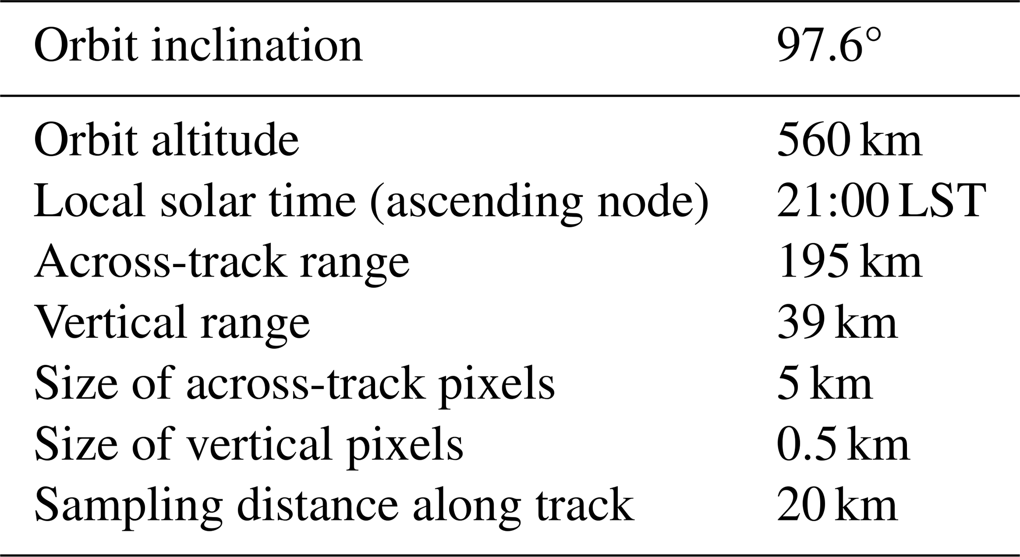
A simple orbit simulator for a circular orbit is used to simulate the MATS tomography grid, i.e. a three-dimensional latitude–longitude–height grid with corresponding local (x, y, z) distances in kilometres. HIAMCM output fields, including temperature, pressure, wind, and density, are interpolated onto this grid. The simulator's calculations are based on a spherical, homogeneous, point-mass Earth model without orbit precession. Parameters were determined from preliminary orbit properties before MATS was launched. They vary slightly from those of the final orbit of MATS, which ended up at 17:30 LST (local solar time; ascending node) and an altitude of 590 km. When designing a telescope, one must compromise between the field of view and the resolution/sensitivity. MATS, which also considers smaller horizontal structures than those represented in the HIAMCM, was designed to prioritize resolution, especially in the vertical direction – nonetheless, it maintains a reasonably wide field of view. The output from the MATS tomography may vary in resolution and dimension, both geographically and in time, as the settings of the instrument may be adjusted based on external factors. However, the resolution and dimension of the temperature grid used in the current analysis are representative of the estimated output from the MATS tomography. The temperature data are expected to be obtained between 70 and 110 km at a vertical resolution of 0.5 km. Regarding the across-track dimension, we expect approximately 200 km of data with a resolution of 5 km. The along-track resolution is expected to be 20 km. As of January 2024, the tomography is still under development, and the sampling used in the orbit generator still provides a good estimate. In Table 1, the properties used for the orbit simulator are shown. An example of the resampled temperature fields can be seen in Fig. 1, where the (x, y, z) directions are illustrated.

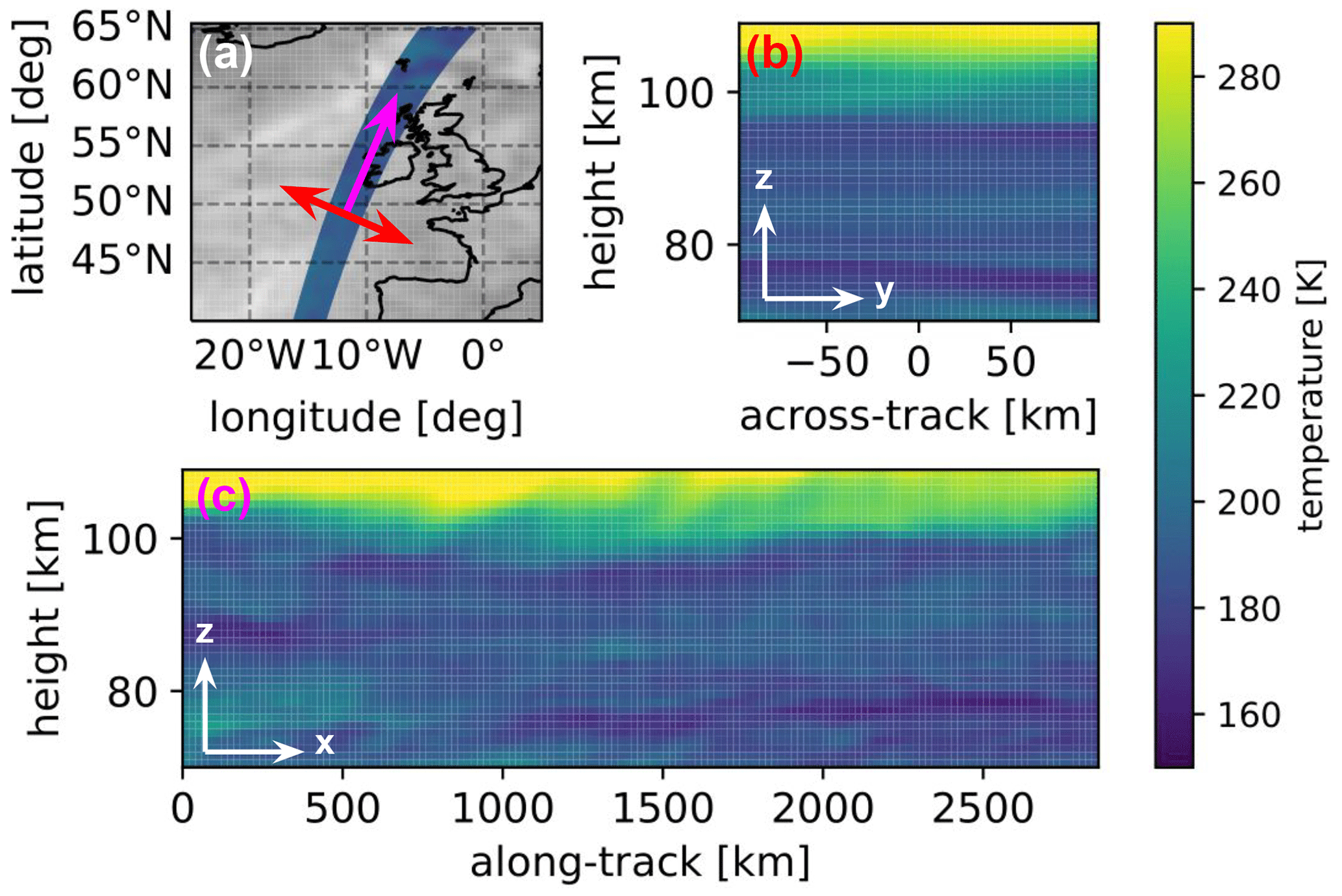
Figure 1 Plots showing the HIAMCM output resampled onto the MATS tomography grid. (a) The orbit swath, with resampled temperature, off the coast of the British Isles. The arrows illustrate where the slices in the accompanying plots are taken. (b) A yz slice taken in the across-track direction of the orbit swath. (c) An xz slice taken in the along-track direction.

Table 1 Properties used in the orbit simulator for generating the MATS tomography grid.

2.4 S3D

S3D is a wave analysis method based on sinusoidal fits developed at Forschungszentrum Jülich in Germany (Lehmann et al., 2012). Residual temperature fields containing waves are divided into overlapping analysis volumes, and in each volume, waves are identified using an iterative 3D sinusoidal-fit technique based on least-squares criteria. These analysis volumes are also referred to as cuboids. Once a wave is identified in a cuboid, the wave is subtracted from the data, and the sinusoidal fit is repeated (typically three times) so that for each cuboid, three dominant waves and their properties are identified. Naturally, S3D cannot identify waves with wavelengths much longer than the cuboid size, and the selected cuboid size thus limits the waves that can be detected. To detect a wave, S3D typically requires the cuboid to contain at least one-third of a wavelength in each dimension. It can thus identify wavelengths of up to 3 times the cuboid's size (Preusse et al., 2012). Combining the wave parameters with background parameters, the total GWMF can be calculated (Eq. 4). The GWMF in the MLT can be captured well by applying S3D to temperature residuals obtained from global zonal-wavenumber decomposition (Chen et al., 2022). In the same study, analysis volumes of 600 km × 600 km × 20 km and 300 km × 300 km × 15 km were used to retrieve the GWMF at altitudes of 75 and 130 km, respectively. Ideally, cuboids should be large enough to capture all of the significant wave momentum but not so large that they lose spatial information by mixing wave parameters from a large altitude range. The dimensions of the MATS tomography output limit the sizes of the S3D analysis volumes that can be used in the operational wave analysis. Specifically, the across-track dimension is the source of the bottleneck as it only has a range of ∼200 km. Due to the large horizontal wavelengths of the waves represented in the HIAMCM, cuboid sizes should span the entire across-track range while maintaining a large along-track range. Vertically, the cuboid size is selected to be slightly smaller than that used in Chen et al. (2022). With a smaller size, vertical variations in wave properties can be obtained at a higher resolution. The cuboid sizes are therefore chosen to be 600 km × 190 km × 10 km (along-track direction × across-track direction × vertical direction). This has the additional advantage that the number of points along the horizontal directions (31 × 39 × 11) is of similar order because of the different sampling rates for the across-track and along-track directions. Each cuboid will be aligned with the centre of the across-track range of the data, with overlapping cuboids positioned every 100 km in the along-track direction. This leads to large overlaps between cuboids along the track, but as waves are not defined at a point, it is natural to analyse them in such a manner. The large along-track extent helps to correctly capture wave parameters, while the overlap allows for the analysis of spatial changes at a reasonably high resolution. Vertically, analysis cuboids are positioned every 5 km between the altitudes of 80 and 100 km. Using these analysis cuboids, the wave vectors are identified. These vectors are then used in a so-called refit, where the vertical extent of the cuboids is reduced to 3 km to accurately determine the wave amplitudes at the centre of each cuboid.

2.5 Savitzky–Golay filter

The S3D wave analysis described in the previous section needs the residual temperature field T^′ as an input. It is therefore essential to carry out the temperature field decomposition described in Eq. (1). In our approach, the background temperature $\stackrel{\mathrm{‾}}{T}(x,y,z)$ is estimated by applying a Savitzky–Golay (SG) smoothing filter (Savitzky and Golay, 1964) to the full temperature field $T(x,y,z)$. The smoothing is applied to each dimension independently: first to the vertical direction, then to the along-track direction, and finally to the across-track direction. The temperature residuals are acquired by subtracting the temperature background from the full temperature.

A Savitzky–Golay filter is similar to a rolling-mean filter, but instead of calculating the mean of the data points within the window, a polynomial of a certain order is fitted. If a zero-degree polynomial is selected, the algorithm becomes identical to a rolling-mean filter. For smoothing along the z direction, a polynomial of order p_z,

$$\begin{array}{}\text{(5)}& \stackrel{\mathrm{̃}}{T}\left(z\right)=\sum _{i=\mathrm{0}}^{p_z}{A}_i{z}^i,\end{array}$$

is fitted using a least-squares criterion. This is done over a smoothing window containing n_z temperature points, centred on T(z=z_j). The value of the polynomial at the centre point, $\stackrel{\mathrm{̃}}{T}\left(z_j\right)$, is extracted as the background value, $\stackrel{\mathrm{‾}}{T}\left(z_j\right)$. $\stackrel{\mathrm{‾}}{T}\left(z\right)$ is fully retrieved by shifting the smoothing window, i.e. repeating the process above for every j. The method can be tuned by controlling the orders p_x, p_y, and p_z as well as the smoothing-window sizes n_x, n_y, and n_z. Figure 2 shows how the number of points in the along-track smoothing window controls the shape of the acquired temperature background for p_x=3. The temperature data are arbitrarily selected along the satellite track for illustrative purposes. A shorter window (smaller n_x) results in an estimated background that resembles the original T curve, while a larger window smooths the curve more. In the latter case, the resulting temperature curve resembles the ZWN < 18 background temperature. Near the data boundaries, symmetric intervals are not possible. We then use asymmetric intervals with fewer points between the central point and the data boundary.

The polynomial orders used in this study are p_x=3, p_y=0, and p_z=2. Means (p_y=0) are taken over all of the across-track points since the horizontal scales of the background temperature are assumed to be much larger than the across-track range of the data. ZWN-18 waves correspond to waves with a zonal wavelength of 2200 km at the Equator. As the orders of the polynomials are held constant, an SG filter will be defined by the number of points in the smoothing windows. More specifically, it will be defined by the number of points in the along-track direction, n_x, and by the number of points in the vertical direction, n_z. In the across-track direction, means are taken across all of the points, and hence n_y=41 for all cases.

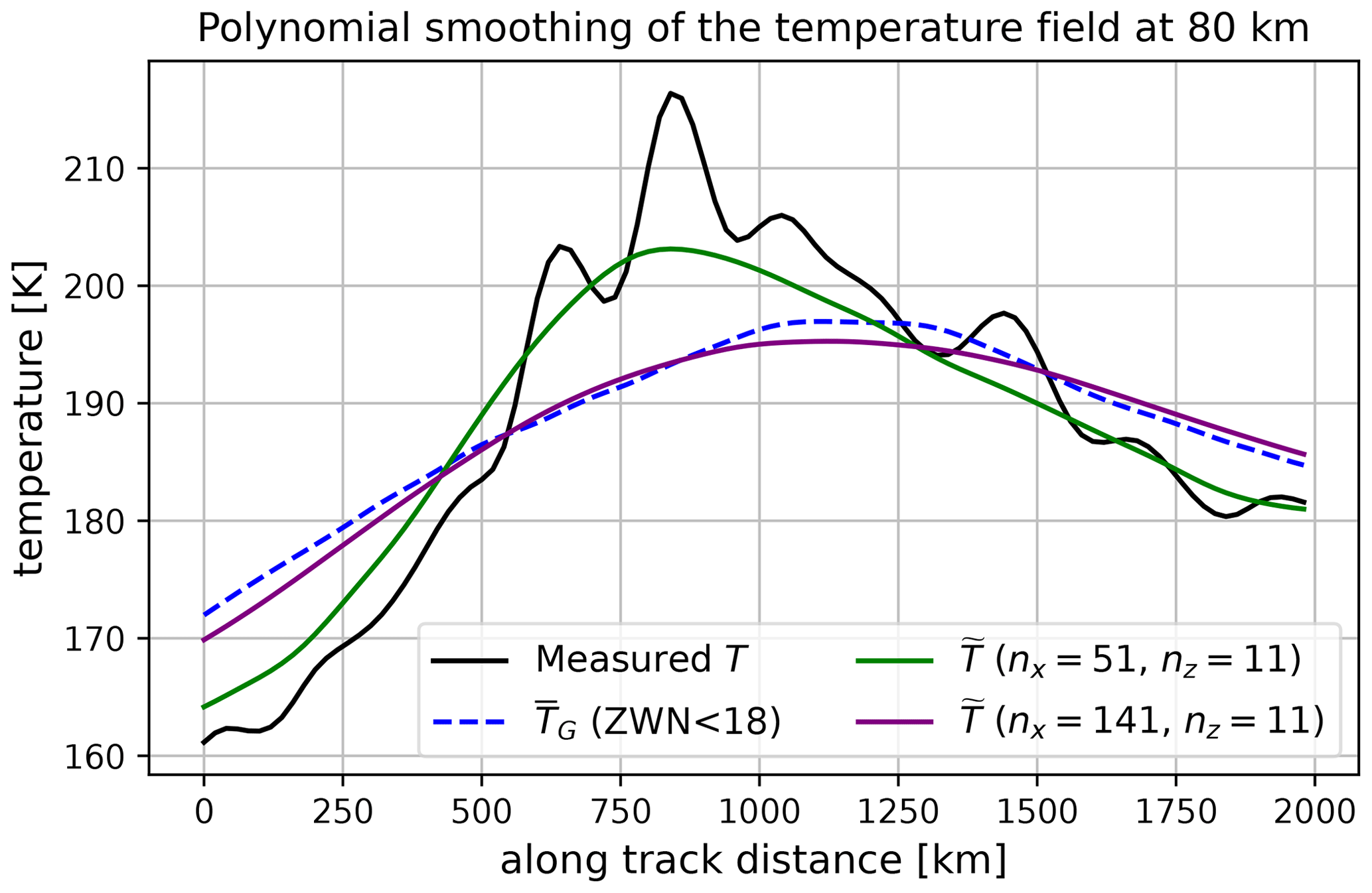
Figure 2 Illustration of two different smoothing lengths in the SG filter. The filter with n_x=51 leads to a temperature background resembling the full temperature. When n_x=141, the obtained curve follows the background obtained from zonal-wavenumber decomposition. In both of the filters, the vertical smoothing is set to n_z=11.

2.6 Averaging kernels and noise

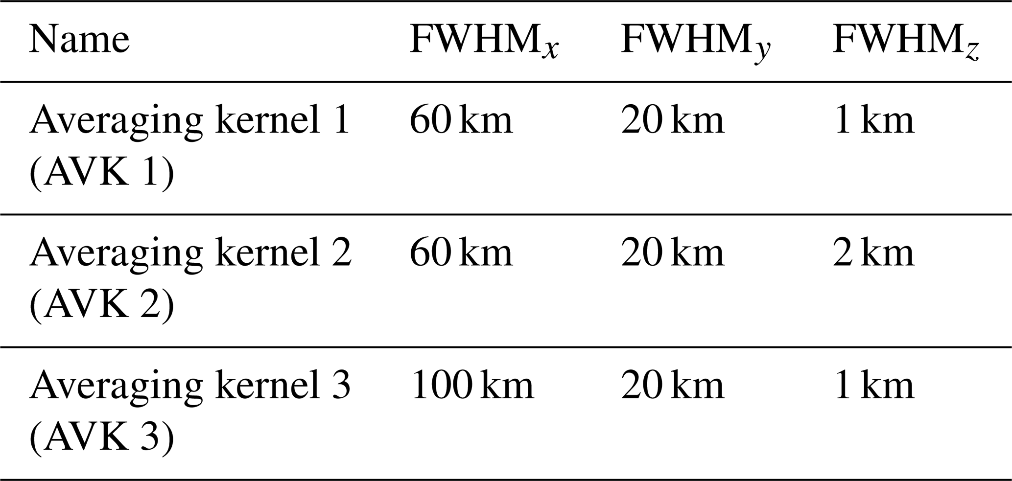
Gaussian white noise and averaging kernels (AVKs) are applied to the synthetic satellite data for a more realistic tomography output, effectively blurring temperatures horizontally and vertically (Rodgers, 2000). The AVKs are applied as Gaussian smoothing curves,

$$\begin{array}{}\text{(6)}& K(\mathit{x},{\mathit{x}}_{\mathrm{0}})=\exp \left(\sum _{i=\mathrm{1}}^{\mathrm{3}}-{\displaystyle \frac{(x_i-x_{\mathrm{0}i}{)}^{\mathrm{2}}}{\mathrm{2}{\mathit{\sigma }}_i^{\mathrm{2}}}}\right),\end{array}$$

where x corresponds to the along-track, across-track, and vertical dimensions $(x_{\mathrm{1}}=x,x_{\mathrm{2}}=y,x_{\mathrm{3}}=z)$ and x₀ corresponds to the central point to which the curve is applied. Moreover, σ_i is the standard deviation along the ith dimension $({\mathit{\sigma }}_{\mathrm{1}}={\mathit{\sigma }}_x,{\mathit{\sigma }}_{\mathrm{2}}={\mathit{\sigma }}_y,{\mathit{\sigma }}_{\mathrm{3}}={\mathit{\sigma }}_z)$. We define each kernel based on its full width at half maximum (FWHM) in each dimension, where FWHM_i $=\mathrm{2}\sqrt{\mathrm{2}\ln \mathrm{2}}{\mathit{\sigma }}_i$. As the final resolution of the MATS tomography output is uncertain, three different AVKs – together covering the expected ranges of the measurement resolution – are applied to the idealized tomography output, $T(x,y,z)$. This results in three different sets of temperature data. The applied AVKs are described in Table 2.

Table 2 The width of the averaging kernels used to generate the synthetic MATS tomography output.

The Gaussian white noise is added with a standard deviation of 5 K based on uncertainty estimates (Gumbel et al., 2020). Structured noise (e.g. stray light), which could appear in the raw images taken by MATS and then propagate into the tomography, is neglected. Such features are assumed to have been removed in the earlier stages of the data processing as they are difficult to predict and properly account for.

3 Analysis chain

The analysis is presented step by step in Fig. 3. As introduced in Sect. 2.1, to evaluate S3D as the operational tool for deriving MLT wave dynamics from the MATS tomography output, two GWMF datasets are produced – one derived from wind residuals and one derived from temperature residuals. For both of these sets, GW-induced perturbations are isolated from the global HIAMCM data using zonal-wavenumber decomposition at ZWN 18. These separated fields include the wind residuals ($u_{\mathrm{G}}^{\prime }$, $v_{\mathrm{G}}^{\prime }$, $w_{\mathrm{G}}^{\prime }$), background density (${\stackrel{\mathrm{‾}}{\mathit{\rho }}}_{\mathrm{G}}$), background temperature (${\stackrel{\mathrm{‾}}{T}}_{\mathrm{G}}$), and residual temperature ($T_{\mathrm{G}}^{\prime }$); the subscript G indicates that the field is derived from global-scale separation. As both wind and temperature residuals are present, the GWMF representations described in Sect. 2.1 can be used equally – i.e. deriving GWMF straight from $u_{\mathrm{G}}^{\prime }$, $v_{\mathrm{G}}^{\prime }$, and $w_{\mathrm{G}}^{\prime }$ (Eq. 3) and deriving GWMF from wave parameters (Eq. 4). The GWMF from wind residuals is referred to as “Reference (wind residuals)”, and its derivation is illustrated by the black arrows in Fig. 3. The zonal mean of the GWMF derived from global wind residuals is considered a “true” reference in that it accurately captures how much momentum is present in the model data, as discussed by Chen et al. (2022). The GWMF derived from the ${\stackrel{\mathrm{‾}}{T}}_{\mathrm{G}}$ temperature residuals, referred to as “Reference (ideal)”, is obtained by first resampling the separated temperature fields to the geometry of the MATS tomography grid using the orbit generator and then applying S3D. Its derivation is illustrated by the blue arrows in Fig. 3. The comparison between these two sets is presented in Sect. 4.1.

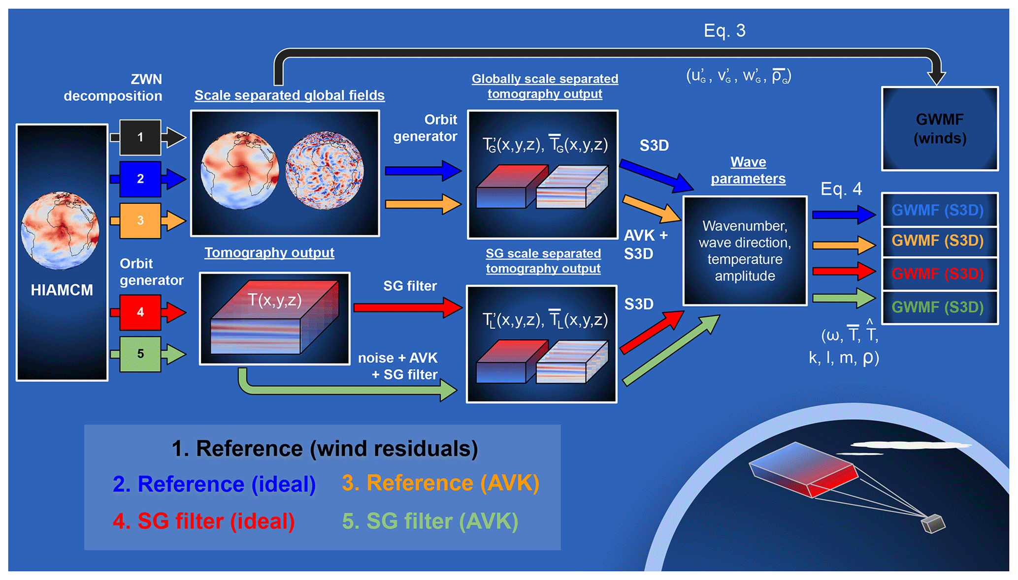
Figure 3 A schematic showing the analysis procedure. Five analysis chains are presented. The steps taken to investigate S3D as an operational wave analysis tool are illustrated by the black and blue arrows. The orange, red, and green arrows show the steps taken to explore SG filtering as a method for local-scale separation in the MATS temperature data.

To investigate the SG filter as a tool for scale separation, the full temperature field T is resampled using the orbit generator. The filtering is then studied using two alternative approaches. In the first approach, the filter is applied directly to $T(x,y,z)$. This is illustrated by the red arrows in Fig. 3. This dataset will be referred to as the “SG filter (ideal)” set as the temperature field is perfectly captured without any simulated degradation from MATS retrieval. For scale separation to be successful, we expect the wave spectra in the residual field to agree with the wave spectra of $T_{\mathrm{G}}^{\prime }(x,y,z)$. The SG filtering is thus evaluated by comparing the SG filter (ideal) set with the GWMF and wavenumber spectra from the Reference (ideal) set. The investigations into idealized SG filtering are presented in Sect. 4.2.

In the second approach, more realistic, simulated MATS tomography outputs are generated. These are referred to as the “SG filter (AVK)” sets, and their derivation is illustrated by the green arrows in Fig. 3. The realistic sets are put through an extra couple of steps, applying Gaussian noise and AVKs to $T(x,y,z)$ before applying the SG filter. It is important to note that when AVKs have been applied to $T(x,y,z)$, we no longer expect the GW spectra of the temperature field to be the same as averaging kernels effectively smoothen the dataset so that small scales disappear. New references are thus required, and these are generated by applying the same AVKs to $T_{\mathrm{G}}^{\prime }(x,y,z)$. The generation of these new references is illustrated by the orange arrows in Fig. 3, and they are referred to as “Reference (AVK)”. The results are presented in Sect. 4.4.

As MATS will not be able to measure background density, operationally this will need to be supplied from elsewhere (atmospheric model, complementing measurements, etc.). In the current investigations of scale separation, background density is estimated by resampling the HIAMCM density onto the orbit grid and applying the same SG filters used for the full temperature. For all of the reference datasets, the background density is retrieved from global-scale separation.

To summarize, the different products described above are compared as follows:

1. The performance of the S3D wave retrieval is evaluated by comparing sets derived from global-scale separation – Reference (ideal) and Reference (wind residuals).

2. SG filtering of the idealized tomography output is evaluated by comparing SG filter (ideal) to Reference (ideal).

3. SG filtering of more realistic MATS tomography outputs is evaluated by comparing SG filter (AVK) to Reference (AVK).

When we compare datasets by studying the zonal mean of the GWMF, we apply 5° rolling averages over latitude to make data interpretation easier. We also apply 3 km rolling averages in the vertical direction of the GWMF derived from wind residuals. This is done to match the vertical extent of the refitted S3D analysis cuboids.

4 Results and discussion

4.1 S3D performance on the MATS tomography grid

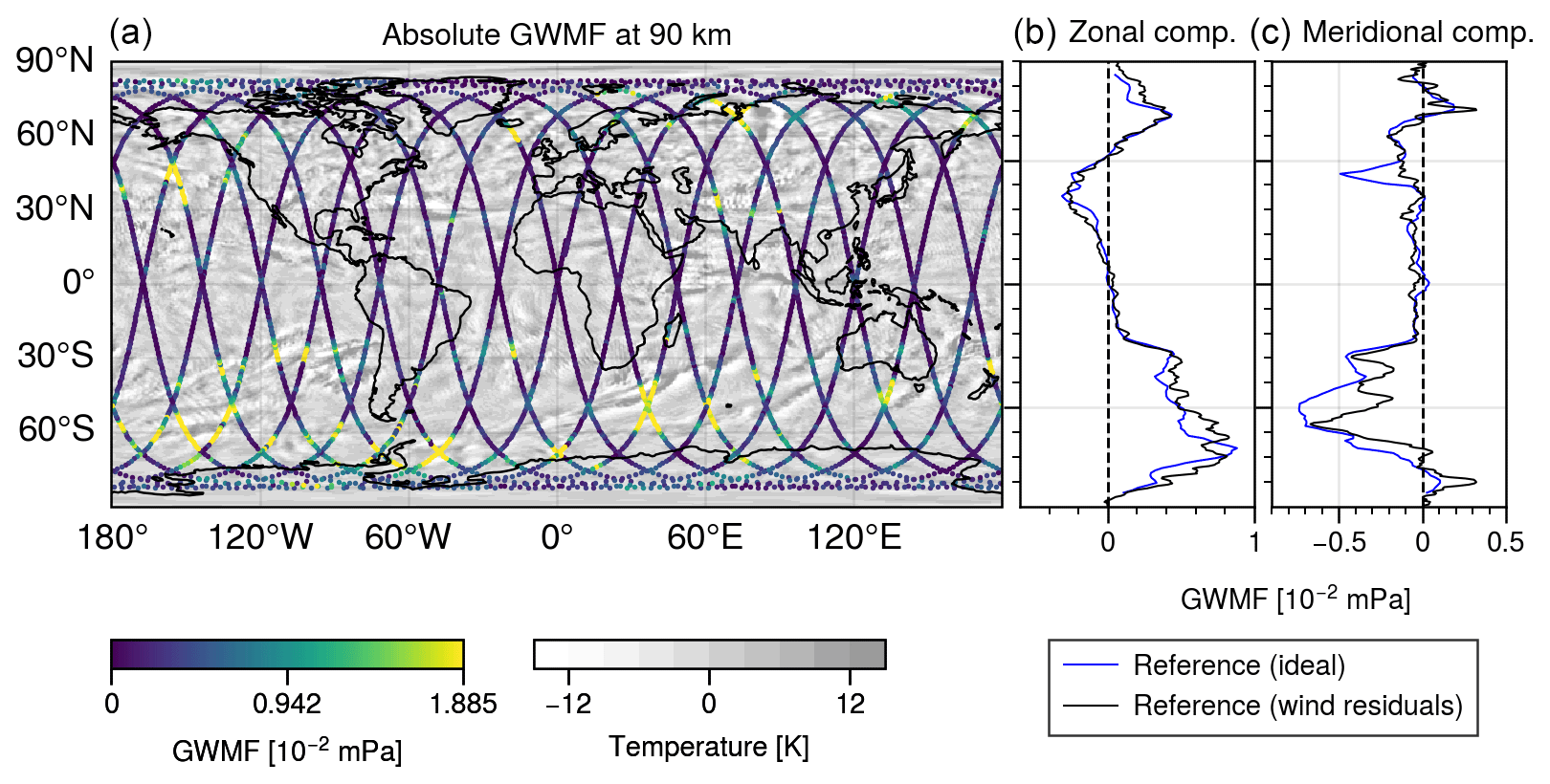
Figure 4 GWMF calculated from a ZWN ≥ 18 residuals. In (a), the MATS orbit swath shows the absolute GWMF at 90 km derived using S3D. The grey-white colour underneath indicates the structures present in the residual temperature field of the HIAMCM. In (b) and (c), the zonal mean of the GWMF from S3D is displayed with the GWMF derived from global wind residuals.

To investigate the performance of S3D on MATS data geometry, we compare the GWMF obtained from the wind residuals ($u_{\mathrm{G}}^{\prime }$, $v_{\mathrm{G}}^{\prime }$, and $w_{\mathrm{G}}^{\prime }$) with the GWMF obtained using derived wave parameters from $T_{\mathrm{G}}^{\prime }(x,y,z)$. In Fig. 3, these are referred to as Reference (wind residuals) and Reference (ideal). Figure 4a shows the absolute GWMF at 90 km, derived using S3D on $T_{\mathrm{G}}^{\prime }(x,y,z)$ along the simulated MATS orbit. Distinctive regions of high GW activity can be identified along the orbit, particularly in the Southern Hemisphere (SH). Figure 4b and c display the zonal means of the directional GWMF from the wind residuals (black) and S3D (blue). In comparing these two representations, for both components of the GWMF, we find that the S3D analysis cuboids capture momentum with high accuracy at most latitudes, with a few exceptions. In the SH at around 50° S, a region of strong GW activity over the Southern Ocean is observed. In this region, the S3D meridional component is partly overestimated compared to the wind-derived counterpart, attributing a stronger flux to the region than what is actually there. On the other hand, the zonal component is underestimated in a region surrounding 60° S, indicating that S3D can both over- and underestimate when compared to the wind residuals. The vertical variations in how well S3D captures GWMF are presented along with the results in Sect. 4.2.

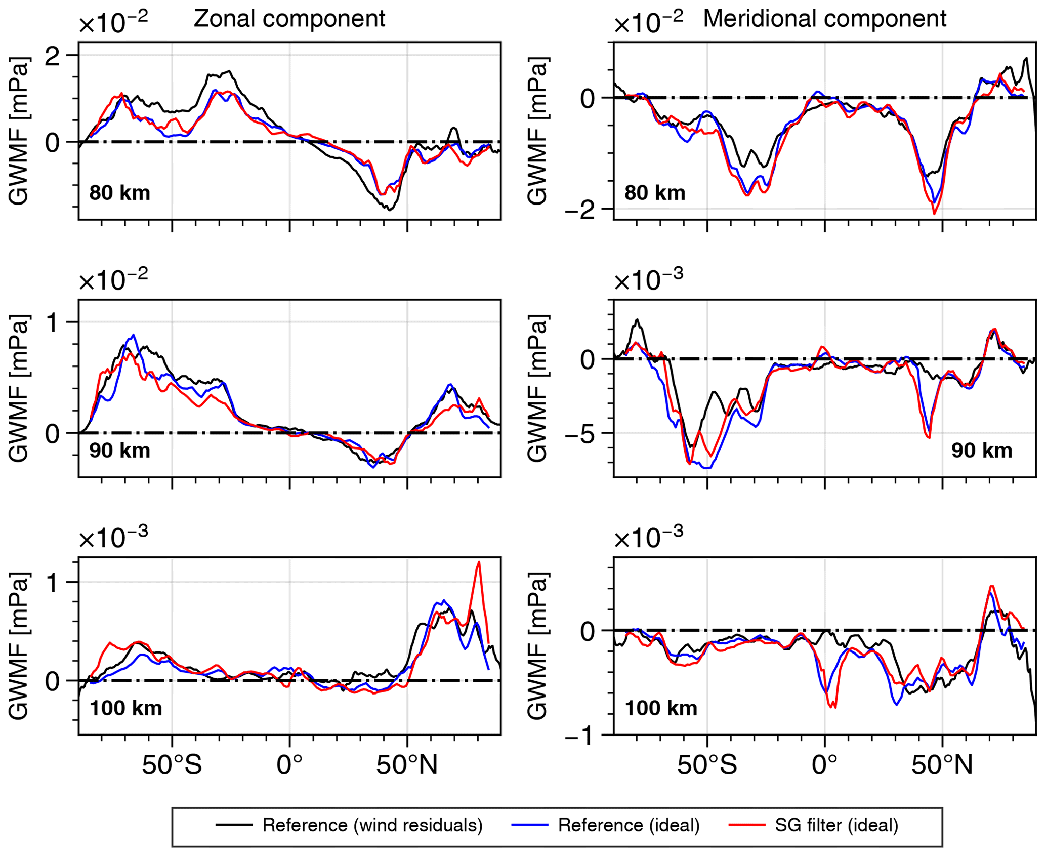
Figure 5 The zonal mean of directional GWMF for different altitudes. Each plot shows the GWMF obtained by applying an SG filter to the idealized tomography output, along with the GWMF references derived from residuals with a ZWN ≥ 18 of wind and temperature.

As both the wind residuals and the temperature residuals are derived from the same global-scale separation, the difference in GWMF mainly arises from the use of S3D on the temperature residuals – some of the difference can be attributed to the sampling difference between the orbit grid and the global model grid, but investigations show that this effect is quite small. At 50° N, the meridional component of the zonal mean of the GWMF is overestimated by S3D. The specific region from which the discrepancy arises is the area of high GWMF in the northern Pacific, just south of Alaska, as seen in the map in Fig. 4. Due to the orbit sampling, this area has a large contribution to the zonal mean, and if it is excluded, the discrepancy disappears. To understand why the disagreement occurs, we visually compared the residual field with the identified waves (not shown). The region in question is characterized by waves with large vertical wavelengths, short meridional wavelengths, and large amplitudes, all contributing to a large GWMF. The large vertical wavelengths appear to be overestimated by S3D, which in turn leads to an overestimation of the momentum flux. Naturally, it is easier to characterize waves that are smaller than the cuboid, and it is not surprising that an area with these large vertical waves is challenging. So while the GWMF derived from the wind residuals – Reference (wind residuals) – accurately captures how much momentum is present in the data, when evaluating SG filtering as a method for scale separation, we cannot expect to approach this “truth” any more closely than what the S3D calculations on the $T_{\mathrm{G}}^{\prime }(x,y,z)$ achieve Reference (ideal). The latter is therefore used as a reference when evaluating how well the local SG-filtering method separates the scales, not the wind-derived alternative.

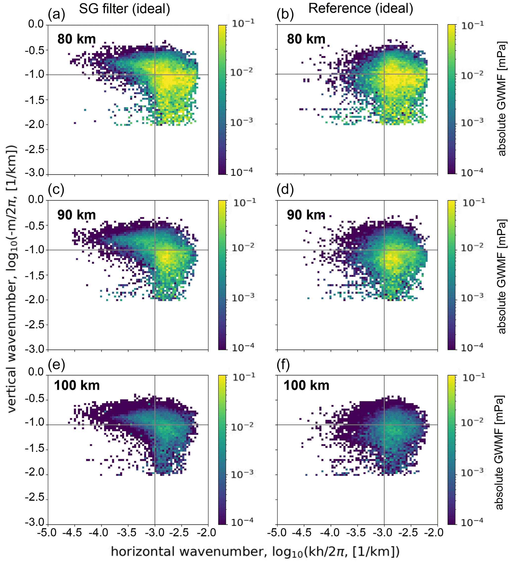
Figure 6 Spectra showing absolute GWMF as a function of horizontal and vertical wavenumbers. In (a), (c), and (e), data are derived by applying the SG filter to the MATS tomography output (SG filter (ideal)). Data in (b), (d), and (f) are derived from the global ZWN decomposition of the temperature field resampled onto the MATS tomography grid (Reference (ideal)).

4.2 Scale separation performance for an idealized product

The GWMF obtained from applying an SG filter to the idealized MATS tomography product – SG filter (ideal) – is shown for several altitudes in Fig. 5 (red lines). Alongside these results, we show the GWMF derived from global-scale separation; both wind residuals, Reference (wind residuals), as black lines; and the temperature residuals $T_{\mathrm{G}}^{\prime }(x,y,z)$, Reference (ideal), as blue lines. As mentioned in the previous section, the latter two are in good agreement, particularly in the middle of the altitude range, as illustrated in Fig. 4. The momentum obtained by applying an SG filter to the temperature field agrees well with the GWMF from the $T_{\mathrm{G}}^{\prime }(x,y,z)$ reference for both components and all considered altitudes. This agreement is particularly strong at 80 km, where the curves follow each other closely, across the latitudes.

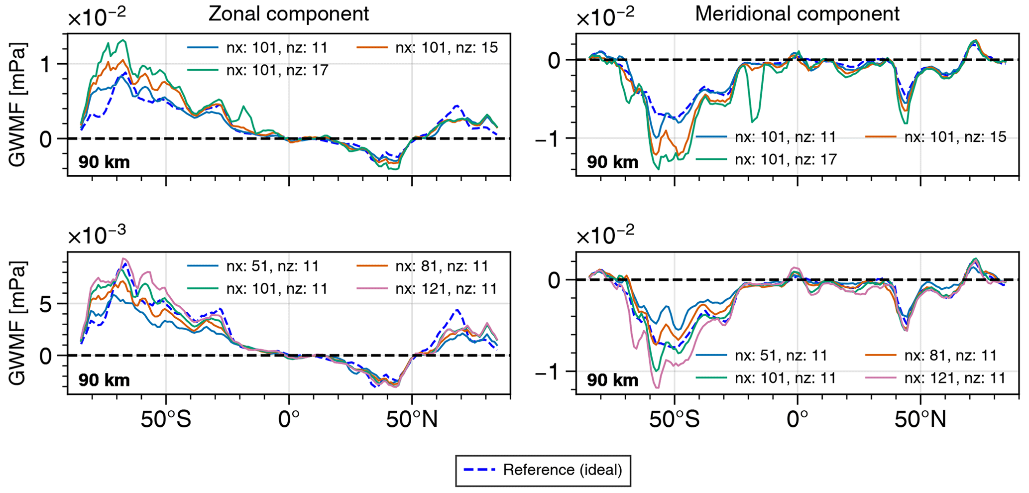
Figure 7 Response of the zonal mean of the GWMF to different smoothing-window sizes in the SG filter. The references display the GWMF calculated from temperature residuals with a ZWN ≥ 18 (Reference (ideal)). Each filter is defined by its number of along-track points, n_x, and vertical points, n_z.

In Fig. 5, SG filtering has been performed using a smoothing-window size of n_x=81 points in the along-track direction and n_z=11 points in the vertical direction. This corresponds to a smoothing-window size of 1600 km in the along-track direction and 10 km vertically. The successful reproduction of the GWMF across most latitudes confirms a successful separation between the temperature residuals and background at ZWN 18. The momentum is overestimated in the zonal components towards the poles, which is especially evident at the 100 km level. In these polar sections of the orbit, the along-track direction of $T(x,y,z)$ is mainly zonal (see Fig. 4). This can interfere with the polynomial smoothing in the filter as the along-track smoothing has mainly been optimized for the meridional structures. The effect is not as strong at 80 km altitude. The challenge of finding a general SG filter that captures horizontal scales equally well across the studied altitude range of 40 km appears difficult.

To retrieve the GWMF correctly, we need to ensure that the waves carrying a substantial part of this momentum are retrieved well. In Fig. 6, the wavenumber spectra from the S3D reference, Reference (ideal), and the idealized SG filtering, SG filter (ideal), are shown. The momentum peaks and surrounding significant momentum are captured well by S3D from both the $T_{\mathrm{G}}^{\prime }(x,y,z)$ and SG-filtered temperature fields. The spectra obtained through the SG filter contain additional wavelike structures that are not in the wave spectra of the reference, indicated by the elongated “tails” in Figs. 6a, c, and e. These waves have small horizontal wavenumbers and large vertical wavenumbers, indicating they are large-scale structures that get interpreted as waves in the GW spectra. To capture the dynamics, it is important that the wave spectrum, especially where momentum is found, is retrieved without losses. Noting the logarithmic colour scale, it is clear that the missing waves, as well as the introduced waves, only carry a small amount of momentum, which is promising for the separation method.

4.3 Sensitivity and response

The vertical and horizontal smoothing of the SG filter affects the wave spectra and GWMF differently, with a greater sensitivity to changes in the vertical smoothing. In Fig. 7, the response of the zonal mean of the GWMF to smoothing-window changes is shown from 90 km altitude. The results can be applied to all altitudes studied. Figure 7 illustrates that fewer points in the smoothing window typically result in a lower GWMF. For a shorter interval, the estimated temperature background will include more of the GW-induced perturbations, thereby leaving less variation for the wave analysis. Vertical smoothing has a substantial effect on the data; a small reduction in the number of points in the vertical-smoothing interval significantly affects the momentum flux. This is not surprising as the vertical resolution is close to the length scales of the vertical wavelengths in the data (the HIAMCM has an approximate vertical resolution of 600 m below 130 km). Consequently, small changes can cut off significant amounts of momentum.

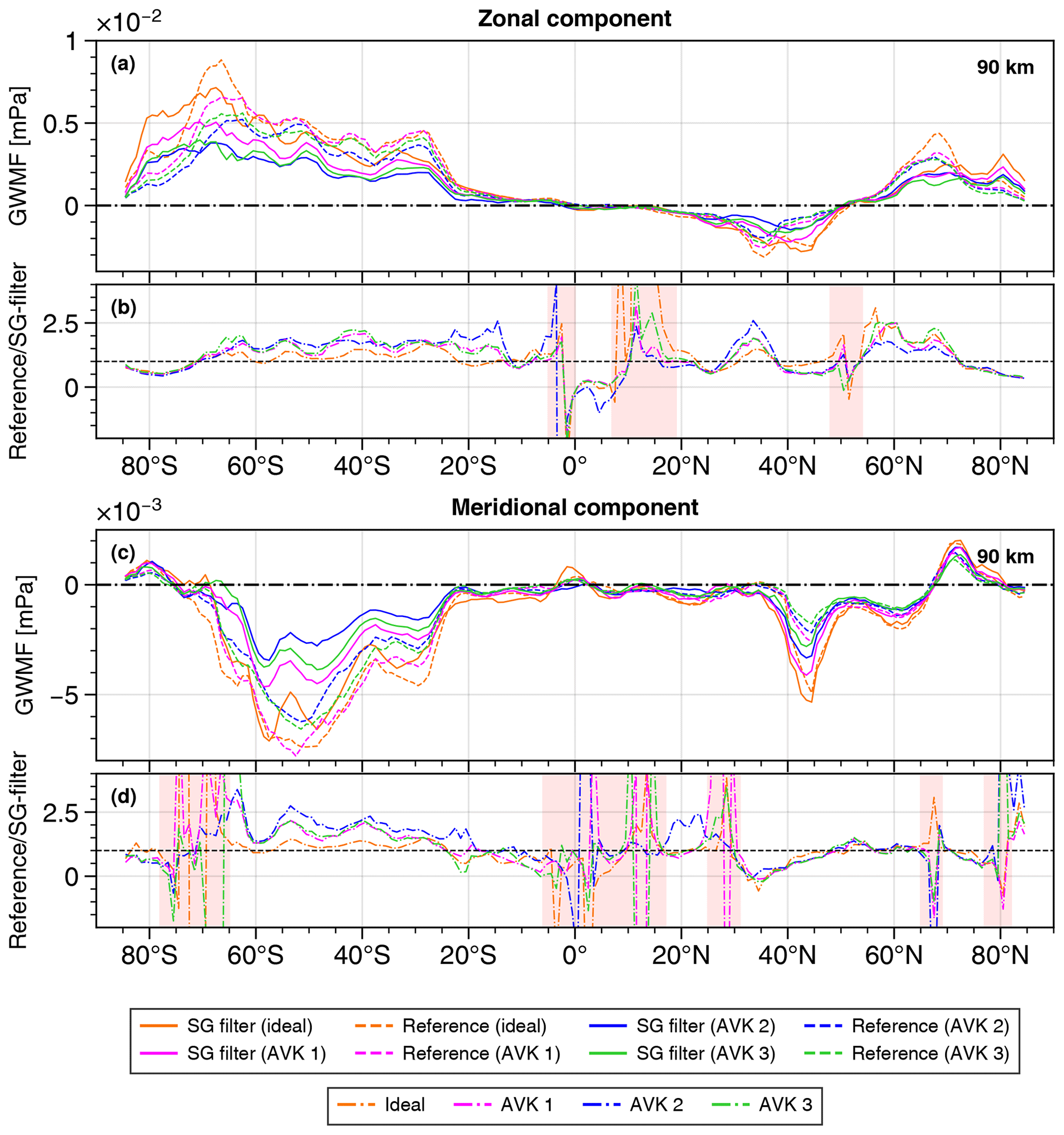
Figure 8 GWMF at 90 km, derived from temperature fields subjected to noise and AVKs, is presented along with corresponding references. The ratios between the two are also illustrated. For segments where the GWMF derived using the SG filter approaches zero, the ratio is highlighted in red. AVK 1: FWHM_x=60 km, FWHM_y=20 km, and FWHM_z=1 km. AVK 2: FWHM_x=60 km, FWHM_y=20 km, and FWHM_z=2 km. AVK 3: FWHM_x=100 km, FWHM_y=20 km, and FWHM_z=1 km.

In general, it should be noted that sensitivity depends on latitude. In the Northern Hemisphere, the response to changes in the smoothing-window size is much smaller. As discussed in Chen et al. (2022), in the Southern Hemisphere MLT region of the considered HIAMCM snapshot, the vertical gradient of the GWMF is strong around 90 km, which is indicative of strong vertical wind gradients and dissipating gravity waves. Nonlinear wave dynamics and short vertical wavelengths make sinusoidal fitting more difficult and thus more responsive to changes in the residual temperature field. As noted in connection with Fig. 6, smoothing may artificially enhance momentum where large-scale structures get interpreted as GWs.

4.4 Scale separation performance for realistic products

We now apply the SG filter from Sect. 4.2 to the more realistic tomography products – temperature fields subjected to Gaussian noise and AVKs. In Fig. 8, the GWMF derived from the filtering of these fields, SG filter (AVK), is displayed as solid lines, and the associated references, Reference (AVK), are displayed as dashed lines. The type of AVK applied is indicated by the colour of the line. The orange lines show the GWMF from Sect. 4.2, which is derived from the idealized tomography product, SG filter (ideal), and its reference, Reference (ideal). Figure 8b and d display the ratios between the GWMF references and the GWMF obtained through SG filtering. Occasionally, the ratios diverge, not because the two zonal means differ much in absolute terms but because the momentum flux derived from applying the SG filter approaches zero. These segments are highlighted in red and should be ignored.

As explained in Sect. 3, the reference zonal means are computed by applying the same AVKs to the residual temperatures $T_{\mathrm{G}}^{\prime }(x,y,z)$ from global-scale separation. By considering the references in Fig. 8, it is clear that the AVKs remove waves in the GW spectra and, consequently, momentum in the zonal mean. For example, in the zonal component (Fig. 8a), the GWMF drops near 70° S, compared to Reference (ideal), for all kernels applied. The largest reduction is seen when the kernel with the largest vertical averaging is applied, namely when FWHM_z=2 km for AVK 2. This illustrates that a loss in the vertical resolution of the measurements has a large effect on the observable waves. Similar conclusions can be drawn from the meridional component of the momentum flux by considering the reference zonal means in Fig. 8c.

Optimized for the idealized tomography product, the SG filter is most effective when no AVKs are applied. In the Southern Hemisphere, the ratios displayed in Fig. 8b and d show that without data degradation, the reference is within a factor of 1.5 of the momentum obtained through SG filtering (orange lines). In the Northern Hemisphere, the results are slightly worse, and the zonal component from SG filtering is partially underestimated (down to half of the reference). Very little GWMF is identified near the Equator and towards the poles; as mentioned in Sect. 4.2, momentum is artificially enhanced.

The performance of the SG filter drops when it is applied to temperature fields subjected to AVKs. This is evident from the ratios, which are further from unity than the counterparts derived from idealized tomography output. In general, the GWMF derived from the filters stays within a factor of 2 of their corresponding references. In the zonal component of the GWMF, scale separation seems equally successful for all AVKs, with some latitudinal variation. In the meridional component, scale separation of the tomography product where AVK 2 was applied was the least successful. This kernel corresponds to the largest loss of vertical resolution. The reason as to why the performance of the SG filter is affected by the kernels is that the AVKs generate a field that is generally smoother. The smoothing windows defined in the filter now capture a background that incorrectly includes some of the larger-scale waves. This is particularly important in the vertical direction, where the FWHM of the kernels is closer to the length scales of the structures. Looking at Fig. 8, it is clear that the difference in along-track averaging between AVK 1, where FWHM_x=60 km, and AVK 3, where FWHM_x=100 km, has little effect on scale separation. Compensation for the smoother temperature field might be possible by revisiting the smoothing-window sizes in the filter. This should be done once the experimental AVKs of the MATS temperature retrieval have been determined. The applied noise may explain some of the lost GWMF, but typically, S3D performs well when noisy data are used. The results in Fig. 8 show the analysis from 90 km, the middle of the vertical extent of the three-dimensional MATS data, but the same conclusions can be drawn from the analysis at 80 and 100 km.

5 Conclusions

In this study, we have shown that the SG filter, which performs local-scale separation based on smoothing polynomials, combined with wave retrieval using S3D, is a suitable operational method for conducting wave analysis on MATS temperature measurements. S3D can characterize and correctly recreate the vertical flux of horizontal gravity wave momentum in both meridional and zonal directions from GWs with wavelengths down to ∼200 km, the lower horizontal wavelength limit of the HIAMCM. The SG filter, considering its simplicity, is a good first candidate for the operational background removal method for MATS as it manages to separate temperature residuals from temperature background on scales equivalent to ZWN-18 structures. The application of AVKs to the measurements, simulating variations in instrument resolution, reduces the performance of scale separation, but the combination of SG filtering and S3D wave analysis should allow the GWMF to be retrieved within a factor of ∼2. Evaluating the methods in this way, by comparing the output to a reference, allows us to find well-suited smoothing parameters, a result that only can be achieved in an ideal model world with full fields and wind data available. Specifically, smoothing-window sizes of n_x=81 points in the along-track direction and n_z=11 points in the vertical direction (corresponding to 1600 km in the along-track direction and 10 km in the vertical direction) capture the dynamics well.

This study was performed using a HIAMCM snapshot from 1 January 2016. To investigate if the method works, a global snapshot from an arbitrary day should be reasonable as it should include regions where analysis might be harder (e.g. in the vicinity of wave breaking) and easier (well-defined wave structures). Nevertheless, for future studies, a larger dataset would be preferable.

The results are a conservative estimate in the sense that in the real MATS measurements, we expect a large fraction of the observed waves to have a smaller horizontal wavelength than what can be observed in the HIAMCM. This will lead to a clearer distinction between waves that carry the majority of the GWMF and the larger scales of the background structures, affecting scale separation positively. At the same time, the temporal sampling will be different, only collecting data at 17:30 and 05:30 LST (at the Equator) due to the sun-synchronous orbit of MATS. This might affect the structure of the large-scale background caught in the measurements. As an AVK is a common diagnostic output from retrieval procedures (e.g. Ungermann et al., 2010), further studies into both observational-filter and S3D settings will continue throughout the tomography development as more information becomes available about large-scale temperatures found in MATS data.

As MATS observes the three-dimensional temperature fields of the MLT, a remaining matter is the acquisition of additional background fields. Background fields of interest for a deeper wave analysis include atmospheric density, required for the GWMF calculations made throughout this study, and background winds, required to perform ray tracing. These additional background fields are not measured by MATS and will need to be incorporated through collaboration with other projects.