the Creative Commons Attribution 4.0 License.
the Creative Commons Attribution 4.0 License.
 | 03 Jul 2024
Toward on-demand measurements of greenhouse gas emissions using an uncrewed aircraft AirCore system
Zihan Zhu
Javier González-Rocha
Yifan Ding
Isis Frausto-Vicencio
Sajjan Heerah
Akula Venkatram
Manvendra Dubey
Don Collins
Francesca M. Hopkins
This paper evaluates the performance of a multirotor uncrewed aircraft and AirCore system (UAAS) for measuring vertical profiles of wind velocity (speed and direction) and the mole fractions of methane (CH4) and carbon dioxide (CO2), and it presents a use case that combines UAAS measurements and dispersion modeling to quantify CH4 emissions from a dairy farm. To evaluate the atmospheric sensing performance of the UAAS, four field deployments were performed at three locations in the San Joaquin Valley of California where CH4 hotspots were observed downwind of dairy farms. A comparison of the observations collected on board the UAAS and an 11 m meteorological tower show that the UAAS can measure wind velocity trends with a root mean squared error varying between 0.4 and 1.1 m s−1 when the wind magnitude is less than 3.5 m s−1. Findings from UAAS flight deployments and a calibration experiment also show that the UAAS can reliably resolve temporal variations in the mole fractions of CH4 and CO2 occurring over periods of 10 s or longer. Results from the UAAS and dispersion modeling use case further demonstrate that UAASs have great potential as low-cost tools for detecting and quantifying CH4 emissions in near real time.
- Article
(3238 KB) - Full-text XML
- BibTeX
- EndNote


Methane (CH4) is a potent greenhouse gas responsible for a quarter of anthropogenic radiative forcing. Increases in agriculture, oil and gas, and waste management activities have contributed to the increase in atmospheric CH4 levels and resultant climate warming (Duren et al., 2019). Due to its relatively short atmospheric lifetime of 10–12 years and high global warming potential of 84 on a 20-year time frame (Myhre et al., 2013), CH4 is an important target for climate mitigation. The Global Methane Pledge of 2021 (IEA, 2022) calls for reductions in CH4 emissions, which will in turn require new measurements of baseline emissions and verification of CH4 mitigation actions. The abatement of human-driven CH4 emissions will take place at individual facilities where local CH4 hotspots have been observed and emissions can be quantified, requiring further measurements to verify the success of mitigation actions.
CH4 emission estimates for individual facilities have been made through observations of wind velocity and CH4 enhancements by mobile vehicle-mounted sensors, which provide the opportunity to survey a large number of facilities in urban or agricultural settings (Moore et al., 2022; Amini et al., 2022; Arndt et al., 2018). Facility-level measurements are particularly needed for dairy farms, which can have a large contribution to CH4 budgets from wet manure management and enteric fermentation emissions and are important for CH4 mitigation plans in California (Marklein et al., 2021). Facilities with large emissions can be identified by atmospheric CH4 enhancements adjacent to or downwind of the source observed from the ground (Hopkins et al., 2016), and then those enhancements can be converted to emission estimates with the addition of local winds. However, vehicle-based studies have been limited by the requirements of site or public road access and often cannot detect emissions from elevated infrastructure such as chimneys and flare stacks. Depending on the distance of the road from the source, the CH4 plume may be lofted high above the mast of an on-road platform, particularly during daytime sampling when the planetary boundary layer height extends on the order of hundreds of meters above the surface.
While airborne platforms do not require road accessibility and are able to provide vertical profiles of CH4, airborne mass balance techniques are limited to isolated facilities in open areas (Hajny et al., 2019; Karion et al., 2013; Kobayashi et al., 2016) and are costly, which limits the potential for repeated sampling to study time-varying emissions. Plume observations made by small uncrewed aircraft systems (sUASs) combine the flexibility of on-road measurements with the vertical profiling capabilities of aircraft. Particularly when used together with on-road sampling to identify hotspot locations, the sUAS is a promising technology for facility-level methane emission estimation. Compared to lightly crewed aircraft and sensor towers, sUASs are low-cost, are portable, and can safely maneuver near emission sources at low altitudes in urban and rural environments. Such characteristics of sUASs are promising for improving the detection of CH4 and CO2 at sub-1 km scales. Higher-resolution observations of CH4 and CO2 can in turn provide more reliable estimates of anthropogenic emission sources that are difficult or infeasible to measure directly as well as detect small plumes that are not resolved by existing remote sensing technologies.
Numerous studies have already explored the integration of low-cost sensors on board sUASs for measuring greenhouse gases. Small onboard sensors (Berman et al., 2012; Golston et al., 2017; Khan et al., 2012; Graf et al., 2018) have successfully been used to measure multiple gas species, including CH4 and CO2. However, low-cost CH4 sensors are in the early stages of development and do not meet the parts per million (ppm) or sub-ppm sensitivity required for environmental monitoring (Honeycutt et al., 2019).
Alternate atmospheric sampling methods have combined the capabilities of multirotor sUASs and higher-precision instruments to obtain more reliable measurements of local greenhouse gas levels. For example, multiple studies have used bag samplers for collecting lower-atmosphere air samples on board multirotor sUASs (Yuan et al., 2021; Nisbet et al., 2020; Shaw et al., 2021). Using this approach, an air volume is captured on board the sUAS and then transported to a location where it can be analyzed using a higher-precision instrument, rendering a single-point measurement for each sampling location. Other studies have aimed to obtain direct measurements of air composition using a sUAS to tow the inlet of a high-precision instrument (Brosy et al., 2017). Although this method can increase the spatiotemporal resolution of measurements, the length and weight of the inlet can limit air sampling operations to a small domain. Therefore, the development of unconstrained air sampling methods that can attain higher spatial and temporal resolution is necessary for accurate characterization of greenhouse gas emissions.
More practical and effective techniques for combining multirotor sUASs and high-precision air sampling instruments may be possible with AirCore technology. To date, passive and active AirCore systems have been developed and deployed on board aircraft (Tadić and Biraud, 2018; Karion et al., 2010), weather balloons (Tu et al., 2020; Sha et al., 2020; Li et al., 2023), and sUASs (Andersen et al., 2018; Vinković et al., 2022). Passive AirCore systems rely on increases in ambient pressure for passive measurements of the atmosphere (Karion et al., 2010). Alternatively, active AirCore systems rely on a micropump and an orifice system to sample air both ascending and descending, as well as moving laterally, which provides an alternate method for increasing the spatial resolution of atmospheric measurements in the lower atmosphere. However, no study so far has explored the integration of multirotor sUASs and AirCore systems for measuring the vertical profiles of wind velocity (i.e., wind speed and wind direction) and air composition simultaneously.
Here, we evaluate the performance of a multirotor uncrewed aircraft and AirCore system (UAAS) for measuring vertical profiles of the atmospheric wind velocity and the mole fractions of CH4 and CO2. The UAAS was designed to measure the mole fractions of CH4 and CO2 in the lower 120 m of the atmosphere. The motion kinematics of the UAAS were also used to infer the wind speed and wind direction while steadily ascending and descending. The UAAS was deployed along with an on-road mobile platform to measure the mole fractions of CH4 and CO2 downwind of dairy farm operations. Finally, the vertical profiles of wind velocity and the mole fractions of CH4 and CO2 were combined with a dispersion model to detect and quantify methane emissions from a dairy farm operation. The findings from field deployments and dispersion modeling are used to assess the effectiveness of the UAAS as a low-cost solution for detecting and quantifying greenhouse gas emission sources.
2.1 Field operations
Four UAAS operations were performed from 20 to 24 January 2020 in the San Joaquin Valley of California to measure CH4 and CO2 downwind of dairy farm operations (see Table 1). CH4 and CO2 surveys were first conducted downwind of dairy farm facilities before each deployment (see Fig. 1a) by sampling through the inlet of a Picarro G1301 cavity ring-down spectrometer (CRDS). The CRDS inlet was placed through the side window of a van driving at a speed of approximately 9 m s−1. The four UAAS deployments were performed at three locations where hotspots of CH4 or CO2 from dairy farms were detected (see Fig. 1a). Before each deployment, an ignited lighter was placed in front of the UAAS inlet to mark the starting point of the measurement interval. During each deployment, the UAAS profiled the wind velocity and the mole fractions of CH4 and CO2 steadily ascending up to a height of 120 m above ground level (a.g.l.) and steadily descending along the same path (see Fig. 1b). The mean speed of ascent and descent flight operations was approximately 0.5 m s−1. The air sample collected on board the UAAS was analyzed within a 5 min period upon landing, also using the CRDS that was employed to conduct mobile surveys. The wind velocity profiles were estimated offline using the flight data collected on board the UAAS autopilot and a kinematic vehicle motion model (González-Rocha et al., 2019).
Table 1Summary of UAAS flight operations conducted in the San Joaquin Valley of California.
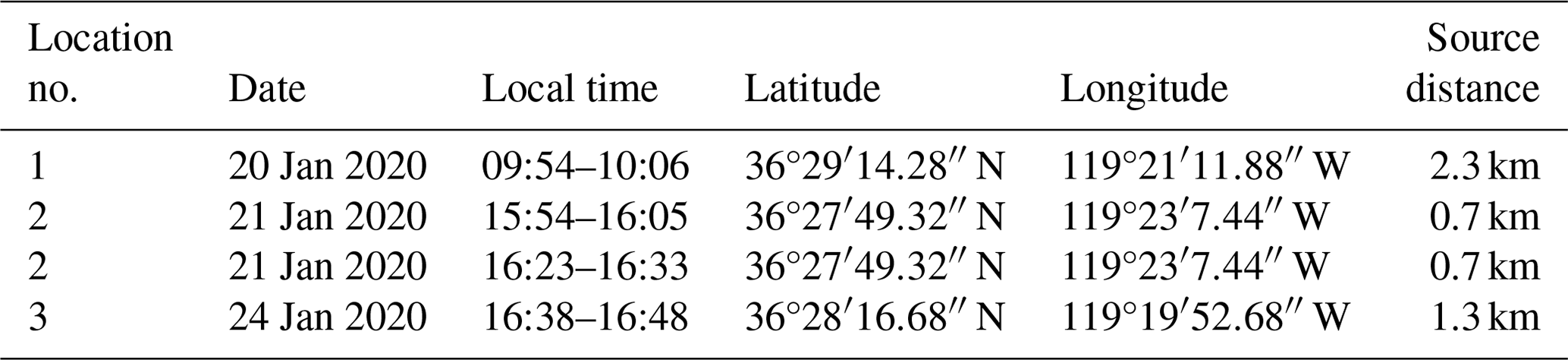
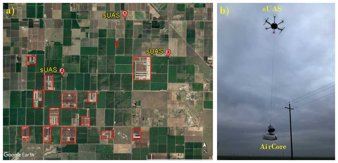
Figure 1(a) A satellite image from © Google Earth showing the livestock facilities surrounding the three locations where UAAS flight operations were performed on 20, 21, and 24 January 2020. (b) A photo of UAAS operations near the surface.
2.2 Ground-based meteorological and gas analyzer instruments
2.2.1 Meteorological evaluation tower
Observations from an 11 m meteorological evaluation tower (MET) were used to assess the performance of the UAAS in measuring wind velocity trends in the lower atmosphere. The MET was located within a radius of 8.3 km from all three UAAS operations. The surface topography between the MET and the locations of the three UAAS operations was relatively flat. As shown in Fig. 2a and b, two Campbell Scientific CSAT3 sonic anemometers were installed on top of the MET at heights of 3 m and 11 m a.g.l. A CR3000 data logger was used to collect and process 1 s and 5 min sonic anemometer measurements. The sonic anemometers and data loggers were both powered using a 12 V marine deep-cycle battery.
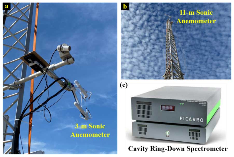
Figure 2(a) An image of the CSAT3 anemometer installed on the MET tower 3 m a.g.l. (b) An image of the CSAT3 anemometer installed on the MET tower 11 m a.g.l. (c) An image of the Picarro G1301 gas analyzer that was used to measure CH4, CO2, and water vapor gas.
2.2.2 Gas analyzer
The gas analyzer used during field experiments is the Picarro G1301 CRDS shown in Fig. 2c. The instrument measures gas-phase CH4, CO2, and water vapor with a varying sampling rate ranging between 0.3 and 1 Hz. During field surveys, the gas analyzer was housed inside a passenger van, and electrical power was supplied to the instrument using a standalone 12 V marine deep-cycle battery with a pure sine inverter. The instrument's precision, flow rate, and pressure while conducting CH4 surveys were measured to be 10 ppb, 0.7 L min−1, and 4.5 mbar, respectively.
2.3 Multirotor sUASs
The multirotor aircraft that was used to tow the AirCore system is a commercially available hexacopter Matrice 600 Pro (SZ DJI Technology Co., Ltd., China). The Matrice 600 Pro airframe measures 1668 mm × 1518 mm × 727 mm and has a maximum take-off payload capacity of 6 kg. The AirCore system was attached to the bottom of the multirotor airframe using a 5 m long stainless-steel cable (see Fig. 1b). Fully integrated, the UAAS has a maximum flight time of 13 min. The flight telemetry record is automatically logged on board the autopilot of the UAAS. The control and retrieval of flight records were conducted using the DJI GO app (SZ DJI Technology Co., Ltd., China).
2.4 AirCore system
2.4.1 Hardware description
The AirCore system consists of perfluoroalkoxy (PFA) coiled tubing that is approximately 60 m long. The coiled tubing has an outer diameter of 12.7 mm, has an inner diameter of 9.53 mm, and can hold up to 4.3 L of air. The inlet of the AirCore system is left open to collect ambient air. The outlet of the AirCore system is connected to a Karlsson Robotics D2028 micro diaphragm pump that weighs approximately 0.3 kg and has a vacuum range between 0 and 406 mm Hg. Airflow through the AirCore system was held constant at approximately 0.45 L min−1 using an O'Keefe Controls no. 9 (0.02286 cm diameter) metal orifice. The metal orifice is located 5 cm upstream of the micro-diaphragm pump as shown in Fig. 3b. The pump and a 12 V lithium-ion battery pack were placed in a plastic enclosure that was positioned in the open area at the center of the AirCore coil. The activation of the AirCore was achieved using a remote relay connected to the pump's power cables. Fully assembled, the AirCore system weighs roughly 5 kg.
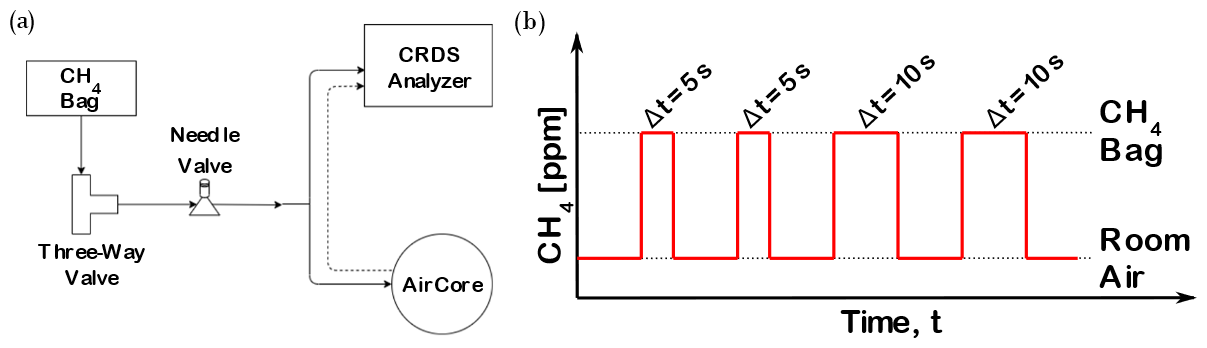
Figure 3(a) A schematic of the AirCore calibration experiment setup. The solid lines and arrows show the gas flow when the CRDS and AirCore sampled the CH4 mixture simultaneously. The dashed lines and arrows show the gas flow when the CRDS pulls air from the AirCore system. (b) A schematic showing the open and closed needle valve position during the AirCore calibration experiment.
2.4.2 AirCore characterization experiments
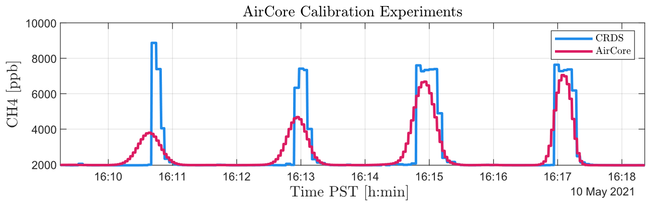
Laboratory tests were conducted to evaluate the performance of the AirCore system for resolving variations in the mole fractions of CH4. We first generated a CH4 mixture by diluting a CH4 standard of 500 ppm inside of a Teflon bag with room air. The Teflon bag was then connected to a three-way valve as shown in Fig. 3a. The three-way valve of the calibration apparatus was controlled to switch between the intake of the CH4 mixture and the ambient air. The AirCore system and the CRDS used in field experiments were connected using a tee junction to pull air simultaneously from the Teflon bag. During the calibration experiment, spikes of CH4 were generated for periods of 5 and 10 s to simulate the AirCore system passing through a CH4 plume (see Fig. 3b). The CRDS provided real-time and continuous measurements of CH4 while the valve was opened and closed and was used to analyze the air sample collected inside the AirCore system.
2.5 Multirotor sUAS wind velocity sensing
2.5.1 Wind estimation method
Wind velocity profiles were estimated using a kinematic model of the UAAS and measurements of attitude and heading that were collected while steadily ascending and descending vertically (Neumann and Bartholmai, 2015; González-Rocha et al., 2019b). The attitude and heading measurements were obtained from the attitude and heading reference system (AHRS) of the UAAS flight autopilot. The AHRS records attitude and heading measurements with a sampling rate of 20 Hz. To develop the kinematic model based on attitude and heading measurements, we first defined a body-fixed reference frame: Fb={b1, b2, b3} at the aircraft center of gravity such that the unit vectors b1 and b2 point along the front and lateral sides of the vehicle, respectively. The unit vector b3 is parallel to the propeller spin axis and points along the direction of the propulsive flow (see Fig. 4a). We also defined an inertial reference frame, Fi={i1, i2, i3}, affixed to the Earth's surface such that the unit vectors i1 and i2 point in the north and east directions, respectively, and the i3 unit vector points towards the Earth's center. The orientation of the body-fixed reference frame is measured relative to the inertial reference frame using the roll–pitch–yaw Euler angles, . After defining the body-fixed and inertial reference frames, two kinematic relationships were derived to infer wind speed and wind direction separately.
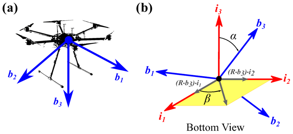
Figure 4(a) A schematic of the sUAS body-fixed reference frame. (b) A schematic showing how the tilt angle, α, and wind direction, β, are computed from the orientation of the sUAS body-fixed frame relative to the inertial reference frame.
Wind speed estimates were inferred from the tilt of the aircraft that is realized in steady-ascending vertical flight to compensate for wind disturbances. The tilt of the multirotor sUAS was determined using the dot product rule:
where
is the rotation matrix mapping b3 from Fb to Fi. In employing this approach, we assume there is a one-to-one relationship between the tilt angle α and the horizontal wind speed (i.e., .
The wind direction was inferred from the projection of the b3 unit vector onto the i1−i2 plane shown in Fig. 4b during a steadily ascending flight. If the aircraft heading is pointing north, wind direction is expressed in the inertial reference frame by computing the four-quadrant tangent inverse of the components of the b3 unit vector projected onto the i1 and i2 unit vectors:
Otherwise, wind direction is expressed in the Earth-fixed reference frame by making the following correction:
2.5.2 Evaluation of multirotor sUAS wind velocity estimates
UAAS wind velocity estimates were validated employing two methods. First, we compared UAAS wind velocity estimates to wind velocity observations collected from the 11 m MET tower described in Sect. 2.2.1. The difference between UAAS and MET tower wind observations was quantified using the root mean square error (RMSE) metric. Second, we compared UAAS wind speed estimates to wind speed profiles obtained from the wind profile power law (WPPL) described in Eq. (5):
where U(z1) and U(z2) are the wind speeds at heights z1 and z2, respectively, and γ is the wind shear exponent value obtained from the MET tower at Z1=3 m and Z2=11 m using Eq. (6):
Results from the two assessments were used to characterize the UAAS wind estimation performance.
2.6 Methane emissions estimates
2.6.1 Dairy farm description
The vertical profiles of wind velocity and CH4 collected during the first flight were used as inputs for a dispersion model to quantify CH4 emissions from a dairy farm. As shown in Fig. 5a, the UAAS vertical profiles were measured at a location that is 1645 m north and 802 m west from the dairy farm, which itself is ∼ 800 m wide. During the first UAAS operation, the wind direction changed from south to north, allowing the downwind and upwind profiles to be collected from a single flight. The methane emission sources on this dairy farm consist of wet manure management in five manure lagoons and enteric fermentation from 3115 milk cows and associated support stock housed in three freestall barns and three cattle corrals (Fig. 5b; Table 2). Surface area estimates derived from Fig. 5b and estimates of the number of animal units derived from permit data (Table 3) were used along with the UAAS vertical profiles to evaluate the effectiveness of the UAAS for estimating CH4 emissions.
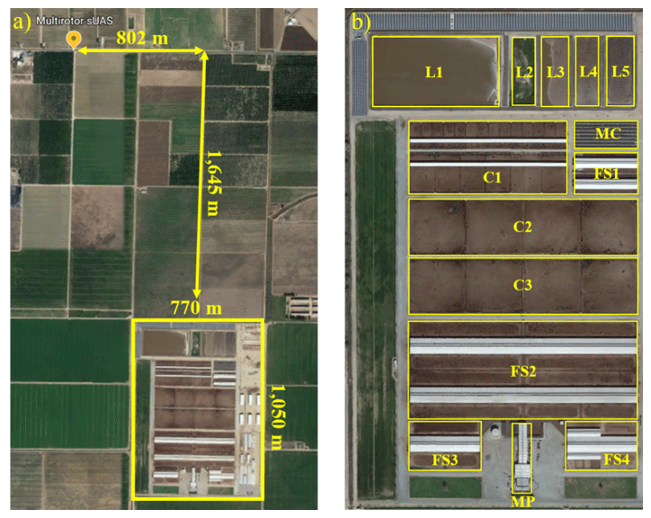
Figure 5(a) A satellite image from © Google Earth showing the location of the first UAAS operation downwind of a dairy farm. (b) A close-up of (a) showing the potential emission sources of CH4 within the farm.
Table 2Dairy farm sections likely to produce CH4 emissions from the enteric fermentation or manure management of approximately 3115 milk cows (Marklein et al., 2021).
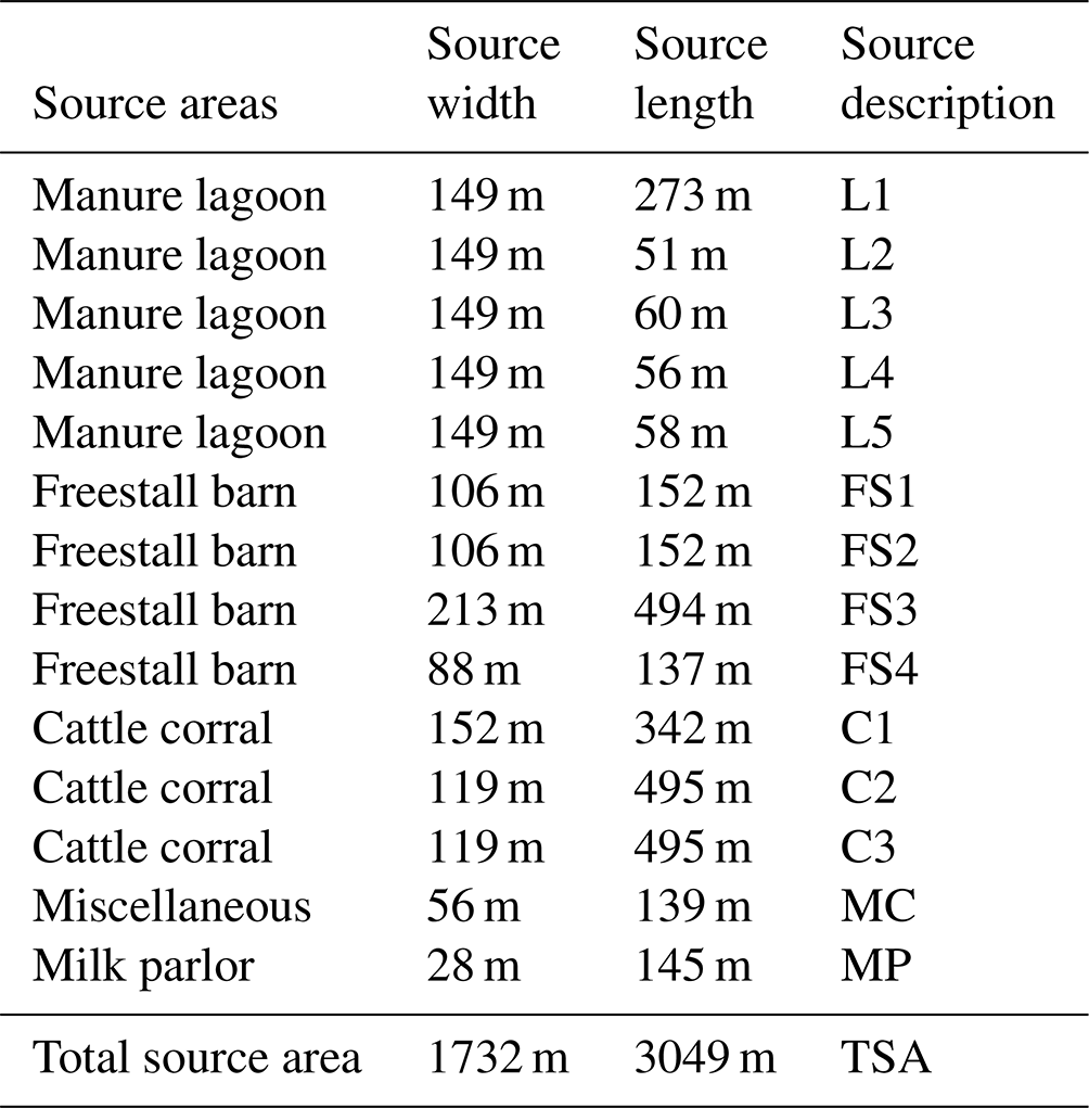
Table 3Calculation for animal units (AU) based on numbers and weights (lb) of different animal classes reported in permit data obtained from the California Regional Water Quality Control Board for the studied farm. The permits report that animals are Holsteins with a milk production of 72 gallons per day.
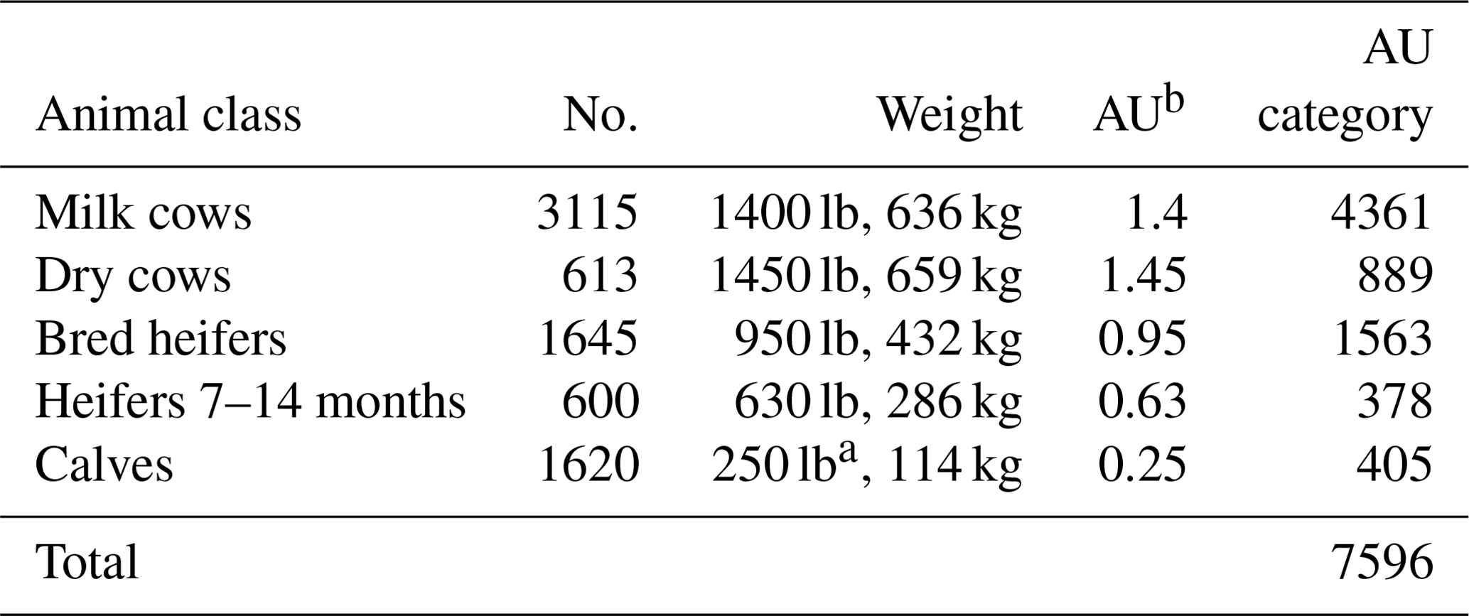
a Assuming median weight for a 4-month-old Holstein calf as in the Penn State Extension growth chart (https://extension.psu.edu/growth-charts-for-dairy-heifers#section-3, last access: 31 March 2024). b 1 AU = 1000 lb live weight.
2.6.2 Dispersion model
The unknown emission rate from the dairy farms can be estimated from atmospheric observations of CH4 through the following relationship:
where Tij is the transport matrix of an area source estimated by Eq. (7) with unit emission rate on data point i. At source j, Cb is the lowest mole fraction of CH4 measured from the UAAS, and Ej is the inferred emission rate obtained by minimizing the residual sum of squares with the constraint that their values are greater than or equal to zero. To achieve this, we use the MATLAB function lsqnonneg described by Lawson and Hanson (1974). The 95 % confidence intervals for the emission rate can be determined by a bootstrapping method which generates a distribution of emission rates by fitting the pseudo-observations to the model estimates.
In the numerical model, the dairy farm can be treated as an area source, which consists of a set of line sources perpendicular to the wind direction. For the contribution from each line source to the receptor, we use an analytical approximation to the integral along the source (Venkatram and Horst, 2006), which gives the concentration as
where
and q is the line source emission rate per unit length; x is the downwind distance of the receptor from the source; y−yi is the distance of the receptor from two end points of the line along the direction parallel to the source; σy is the horizontal plume spread; erf is the error function; and Fz(x,z) is the vertical distribution function, which is applied the numerical solution of the mass conservation equation (Venkatram and Schulte, 2018).
where C denotes the crosswind-integrated concentration for convenience, K(z) is the vertical eddy diffusivity, and U(z) is the horizontal velocity. The boundary conditions are
where z0 is the roughness length, which is computed to be 0.005 m (Qian et al., 2010), and H is the boundary layer height. The numerical method initializes a Gaussian concentration distribution at x=0, which is centered at a source height of zs=0.1 m and with an initial vertical spread σz=0.1 m. Van Ulden (1978) shows that the analytical solution of Eq. (8) provides an excellent description of concentrations measured during Project Prairie Grass (Barad, 1958). Venkatram and Schulte (2018) evaluates the usefulness of the analytical formulas through the numerical solution using the Businger–Dyer expressions for eddy diffusivity of heat (KH(z)) and the wind profile (U(z)).
Four UAAS deployments were performed at three locations in the San Joaquin Valley where CH4 hotspots from dairy farms were detected. During each deployment, the UAAS measured vertical profiles of wind velocity and the mole fractions of CH4 and CO2 while ascending and descending during periods of both variable and relatively stable wind conditions, with each deployment lasting approximately 9 min. All four sets of wind velocity and air composition profiles were evaluated using ground-based measurements. The UAAS measurements and dispersion modeling were combined to estimate the methane emissions from one of the dairy farms.
3.1 Wind velocity profiles
The UAAS was found to reliably measure wind velocity trends while vertically ascending and descending in both variable and relatively stable wind conditions. The comparison of UAAS and MET wind speed observations during variable wind conditions resulted in an RMSE of 1.1 m s−1, with the smallest error being observed while the UAAS ascended and descended near the surface (see Fig. 6a). The corresponding measurements of wind direction from the UAAS and MET were in close agreement near the surface as well. In relatively stable wind conditions, the RMSE between UAAS and MET tower wind speed observations was equal to or less than 0.5 m s−1 (see Fig. 6b, c, and d). Notable differences between UAAS and MET observations of wind direction were observed only at the start of the third flight.
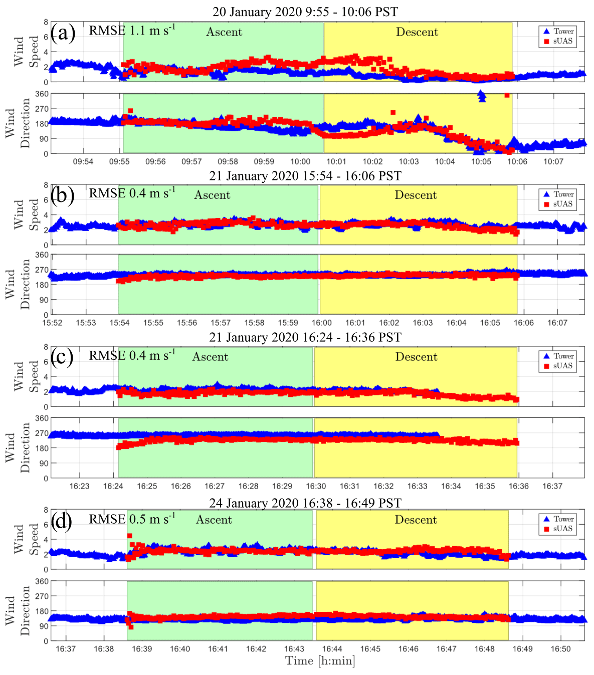
Figure 6A comparison of UAAS (red) and MET (blue) observations of wind speed and wind direction.
The UAAS may also have good performance measuring wind speed while ascending vertically based on the evaluation of UAAS and power-law wind speed profiles. As shown in Fig. 7a, the uncertainty bands of the wind speed profiles that were obtained from the ascent and descent UAAS operations and the power law overlapped up to 120 and 80 m a.g.l., respectively, in variable winds. In relatively stable wind conditions, the uncertainty bands of the wind speed profiles obtained from ascent and descent operation and the power law overlapped up to 110 and 60 m a.g.l., respectively, as shown in Fig. 7b. In both comparisons, the uncertainty band of each power-law profile was computed using the standard deviation of wind velocity surface measurements collected from the 11 m MET tower.
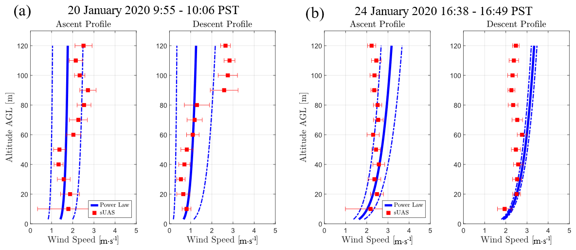
Figure 7A comparison of UAAS and power-law wind speed profiles measured during (a) variable and (b) relatively stable wind conditions. The dashed blue lines show the uncertainty in the power-law wind speed profiles.
3.2 CH4 and CO2 profiles
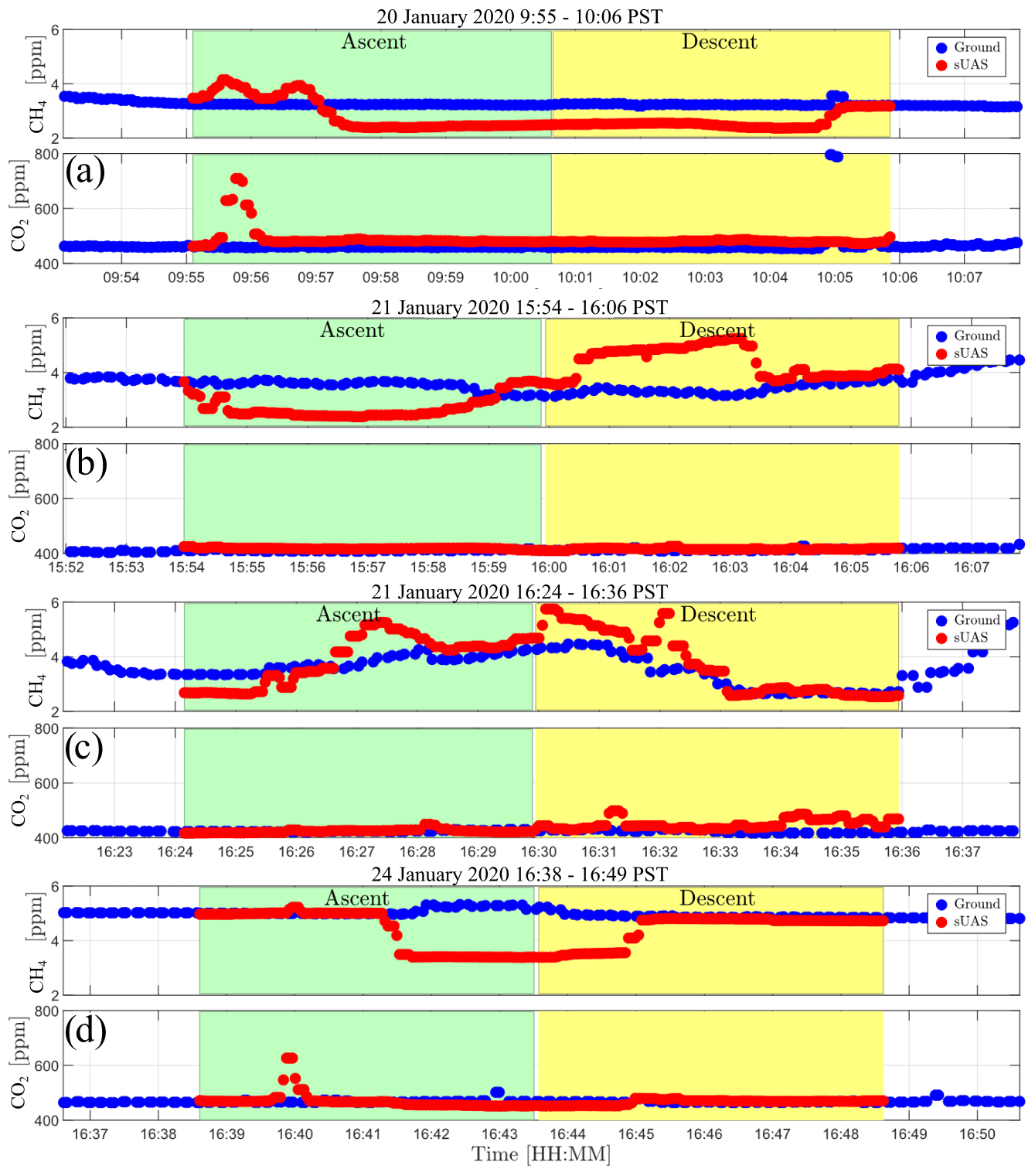
In addition to measuring wind velocity trends, the UAAS measured the mole fractions of CH4 and CO2 during both variable and relatively stable wind conditions. As shown in Fig. 9, the CH4 and CO2 measurements from the UAAS and those from the CRDS when sampling direct surface measurements were in close agreement at both the start and end of the first, second, and fourth UAAS flights, which is when the UAAS and CRDS were closest to each other. During the third flight, as shown in Fig. 9c, only the UAAS and CRDS measurements of CO2 were found to overlap at both the start and end of the UAAS operation. The UAAS and CRDS measurements of CH4 differed by 0.5 ppm at the start of the UAAS flight, which may be due to the separation between the CRDS and UAAS during deployment. Despite the measurement anomaly observed at the start of the flight, the UAAS and CRDS measurements of CH4 were found to follow more consistent trends throughout the remaining period of operation.
3.3 AirCore characterization experiments
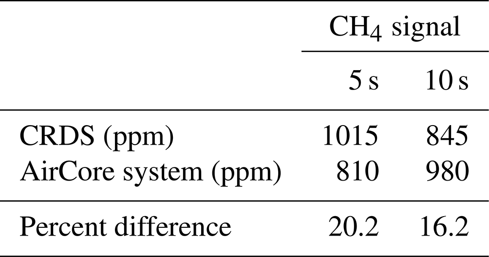
The UAAS was found to accurately resolve two spikes in CH4 that were 10 s long based on results obtained from the characterization experiments performed in a laboratory (see Fig. 8). On the other hand, the UAAS was significantly less accurate measuring two CH4 spikes that were only 5 s long, which is likely due to the UAAS having a slower time response. However, the lesser performance of the UAAS for measuring the spikes in CH4 that were 5 s long may have an insignificant effect on the overall reliability of CH4 and CO2 measurements. As shown in Table 4, the percent differences between the area under the curve of UAAS and CRDS signals were found to be 20.2 and 16.2 when measuring CH4 spikes that were 5 and 10 s long, respectively. From these results, we conclude that the UAAS has a spatial resolution of 5 m while flying at a steady rate of 0.5 m s−1.
3.4 Wind velocity and air composition profiles
As shown in Fig. 10, the UAAS profiles of wind velocity and air composition were found to capture the vertical and temporal variations in CH4 and CO2 plumes that were measured downwind of dairy farm operations. These observations were useful for understanding how the enhancements of CH4 and CO2 varied in the lower atmosphere during periods of both variable and relatively stable wind conditions.
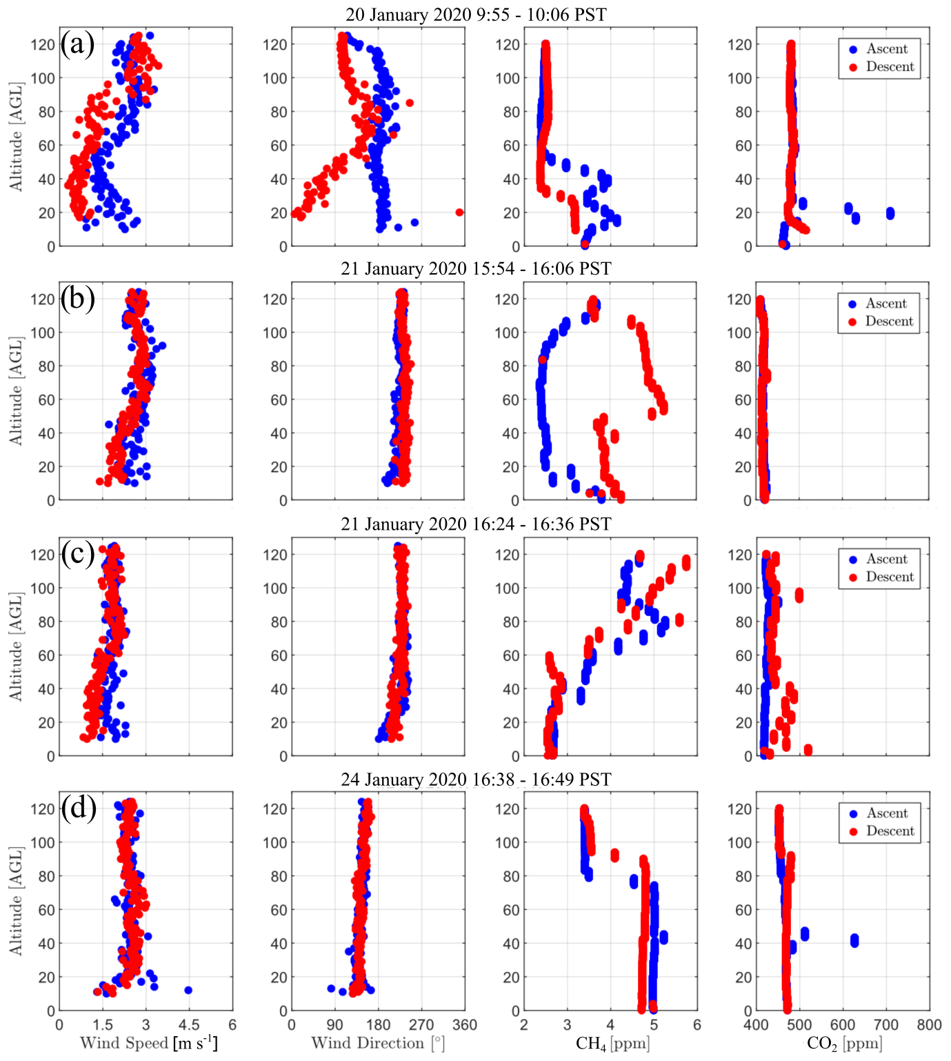
During the first UAAS deployment, CH4 and CO2 plumes were observed close to the ground under variable wind conditions. The observed enhancements of CH4 and CO2 at low altitudes are likely due to UAAS operations taking place in the morning when the boundary layer was shallow and there was minimal vertical mixing. As shown in Fig. 10a, the UAAS ascent measurements captured a 1.5 ppm CH4 enhancement near the ground and up to 60 m a.g.l. A CO2 enhancement of approximately 220 ppm was observed to extend from 15 to 25 m a.g.l. The winds during the ascent fluctuated between 1 and 3 m s−1 from the south, shifting eastward above a height of 117 m a.g.l. The descent measurements captured a 0.7 ppm enhancement of CH4 extending from the ground up to 30 m a.g.l. The winds during the UAAS descent varied between 0.5 and 3 m s−1 while the wind direction rotated from the east to the south and from the south to the north. CH4 and CO2 mole fractions were relatively constant at heights greater than 60 m a.g.l. during the ascent and descent, indicating local background levels above the height of the dairy farm's emission plume.
The second UAAS deployment captured a methane plume moving upward during a period of turbulent conditions and relatively constant winds. As shown in Fig. 10b, CH4 mole fraction enhancements greater than 1 ppm were observed both at the start and end of the UAAS ascent. South-southwesterly winds were observed to gradually increase from 1.5 to 3 m s−1 during this period. UAAS descent measurements show the mole fraction enhancement of CH4 to gradually double from 1.4 to 2.8 ppm before decreasing again as south-southwesterly winds persisted. The enhancements of CO2, on the other hand, were insignificant during the UAAS ascent and descent. The observed differences between the ascent and descent measurements of CH4 provide insight into the dynamic nature of plumes in well-mixed afternoon conditions driven by atmospheric turbulence, which is difficult to obtain using ground-based sensing techniques alone.
The third deployment showed an elevated CH4 plume under constant wind conditions. As shown in Fig. 10c, the CH4 mole fraction was observed to increase from approximately 2.6 to 6 ppm during both the ascent and descent, showing the CH4 plume to vary less significantly with time. The mole fraction enhancements of CO2 were greater than 50 ppm only below 40 m a.g.l. during the descent. Southwesterly winds were observed to gradually increase as the height increased from 1 to 2.5 m s−1 during both the ascent and descent.
The fourth deployment captured consistent CH4 enhancements downwind of a dairy farm extending from the surface up to 80 m a.g.l., with a marked drop in enhancements above 100 m (see Fig. 10d). CH4 mole fraction enhancements of 1.7 and 1.5 ppm were observed up to heights of 75 and 80 m a.g.l. during the ascent and descent, respectively. The mole fraction of CO2 was observed to increase briefly from 480 to 620 ppm at a height of 40 m a.g.l. before returning to a constant value of 480 ppm for the remainder of the UAAS operation. Southeasterly winds varying between 1.5 and 3 m s−1 persisted during both the ascent and descent. The similarity between the ascent and descent profiles measured during the fourth deployment is not surprising for the stable atmospheric conditions expected an hour before sunset.
3.5 CH4 detection and quantification
The vertical profiles of wind velocity and CH4 that were collected from the UAAS operation performed on 20 January 2020 were used as inputs for the dispersion model described in Sect. 2.6.2 to quantify CH4 emissions from an isolated dairy farm. We selected this set of measurements for two key reasons: (1) the wind conditions during the UAAS operation shifted from south to north, making it possible to obtain upwind and downwind CH4 measurements from a single flight, and (2) the UAAS was able to fly high enough to measure the height of the CH4 plume and the CH4 background (the latter was determined from the air sample collected 120 m a.g.l.).
To detect CH4 emissions from the nearby dairy farm, UAAS measurements of wind speed and wind direction were used with the dispersion model to generate a footprint map of CH4 emissions. As shown in Fig. 11, the dairy farm operation, which is denoted by a white rectangle, is well within the area having the highest contribution to the CH4 mole fraction measured at the receptor (i.e., the UAAS). After generating a footprint map, UAAS profiles of wind velocity and CH4 were used as dispersion modeling inputs to compute dairy farm emission estimates. Results from this analysis show that whole-farm emissions for this dairy farm were on average 226 kg h−1, with a lower limit of 140 kg h−1 and an upper limit of 277 kg h−1.
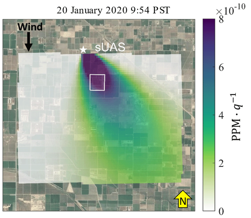
Figure 11A satellite image from MathWorks® overlaid with the footprint map obtained from the dispersion model. The white star shows the location of the UAAS operation and the white rectangle shows the location of the upwind dairy farm. The black vector shows the prevailing meteorological wind direction measured during the ascent of the UAAS operation. The color bar units are in ppm per unit of emission.
Four UAAS deployments were successfully performed in the San Joaquin Valley to measure vertical profiles of wind velocity and the mole fractions of CH4 and CO2 downwind of dairy farm operations. We evaluated the reliability of the UAAS measurements using ground-based MET and CRDS observations. We also used the UAAS measurements of wind velocity and air composition to evaluate the enhancements of CH4 and CO2 during periods of both variable and relatively steady wind conditions. Lastly, we combined UAAS measurements and dispersion modeling as part of a use case study to determine the utility of UAAS datasets for detecting and quantifying CH4 emissions from a dairy farm operation. From this single use case that met the requirements of emission estimation (i.e., observation of an isolated plume downwind of a nearby dairy farm where the farm falls entirely within the footprint of the observation and background CH4 levels are also measured), we estimated facility emissions of 5430 kg d−1 (with a range of 3370–6660 kg d−1). This range overlaps with the yearly estimated methane emissions for this particular farm of 3950 kg d−1, assuming emissions are evenly spaced over the course of a year, from a model that accounts for the number of cows and manure management practices (Marklein et al., 2021). After normalizing for herd size, our estimated emissions of 714 g AU−1 d−1 (range of 444–876) are similar to those measured in wintertime at another California dairy farm with comparable management practices, i.e., 752 g AU−1 d−1 (range of 700–803) (Arndt et al., 2018).
We found the UAAS to provide reliable measurements of wind speed and wind direction in both variable and relatively steady wind conditions. During variable wind conditions, the UAAS and MET observations of wind speed and wind direction were consistent when the height difference between the two systems was less than 50 m. More significant differences observed aloft between the UAAS and wind speeds derived from power-law analysis of MET observations were likely due to wind shear. During periods of relatively stable wind conditions, the UAAS and MET observations of wind speed and wind direction were consistent up to heights of 60–80 m a.g.l. However, a more thorough comparison of UAAS and ground-based wind observations is required to assess if the wind speed errors observed aloft are the result of extrapolation errors associated with the wind profile power law and to determine the full range of wind conditions for which the wind estimation scheme used to infer wind velocity is reliable. Overall, we expect the wind speed estimation errors to increase as wind conditions intensify since the tilt range of the aircraft is reduced by the added payload weight.
In addition to providing observations of wind velocity, the UAAS was effective in measuring the mole fractions of CH4 and CO2 in the lower atmosphere. UAAS and ground-level CRDS measurements of CH4 and CO2 were in close agreement when the UAAS operated near the surface while both ascending and descending in variable and relatively steady wind conditions. Results from the laboratory AirCore characterization experiment also demonstrated that the UAAS can accurately resolve CH4 variations occurring over a period of 10 s or longer. Resolving variations at the 10 s scale is important for both reducing the uncertainty in CH4 and CO2 emission estimates and extending the spatial coverage of UAAS operations. Furthermore, we found that the smearing effects produced by fast CH4 variations led only to a 5 % difference in the area under the curve of the 5 and 10 s long CH4 signals. The latter finding suggests that smearing effects may only have a small impact on the accuracy of CH4 and CO2 column measurements.
Future work will address a number of limitations that were encountered while validating UAAS wind velocity measurements. First, UAAS flight operations will be conducted next to conventional in situ and remote wind sensors (e.g., mast towers and lidar instruments) to better characterize the uncertainty in UAAS wind estimates. More sophisticated dynamic models will also be explored as a means to increase the accuracy of wind estimates, both ascending vertically and moving laterally. Previous studies have shown that dynamic models can render higher-fidelity wind estimates from the motion of sUASs (González-Rocha et al., 2019, 2020). Higher-fidelity measurements of wind velocity and mole fraction measurements obtained from both lateral and vertical profiles will likely lead to improved emission estimates. Combined with vertical profiles, lateral measurements of wind velocity and the CH4 mole fraction can help determine the horizontal spread of CH4 plumes, providing a more robust low-cost method for quantifying emissions fluxes from dairy farms.
Findings from the use case study show that combining UAAS measurements and dispersion modeling can help to detect and quantify CH4 emission from large source areas. The region of the footprint map with the highest CH4 sensitivity was found to overlap with the location of the downwind dairy farm. In addition to aiding in the detection of large emission sources, UAAS measurements and dispersion modeling can provide emission estimates in just hours. In addition to the system design issues that can be improved, these flights provide guidance for the meteorological conditions and spatial considerations for CH4 emission estimation. For example, the comparison of all four sets of profiles shown in Fig. 9 suggests that measurement conditions are most favorable in the morning when the UAAS can fly well above the height of the planetary boundary layer and before the regional signals get mixed.
Overall, we found the UAAS to be a promising low-cost solution for detecting and quantifying greenhouse gas emissions from dairy farm operations. Leveraged with a ground-based mobile laboratory, the UAAS can be deployed at sites where greenhouse gas hotspots are prevalent (provided that airspace access is available). The UAAS measurements of wind velocity and air composition are useful for understanding how CH4 and CO2 enhancements vary with height and time, providing higher-resolution observations for monitoring lofted plumes. Combined with dispersion modeling, UAAS measurements are also useful for detecting and quantifying greenhouse gas emissions from dairy farms. Furthermore, the extension of UAAS capabilities to measure horizontal transects of wind velocity and air composition can help characterize the spatial heterogeneity of large emission sources. This capability can provide a new paradigm for improving bottom-up estimates of greenhouse gas emissions from dairy farm operations and other important sources such as waste landfills, gas and oil fields, and wetlands. Ultimately, more reliable bottom-up estimates of greenhouse gases will lead to more effective mitigation strategies.
We developed and deployed a multirotor uncrewed aircraft and AirCore system to measure vertical profiles of wind velocity and the mole fractions of CH4 and CO2 downwind of dairy farm operations in the San Joaquin Valley of California. Results from field and laboratory performance evaluations show that the UAAS can reliably measure vertical profiles of wind velocity and the mole fractions of CH4 and CO2. Integrated with ground-based mobile sampling strategies, UAAS measurement capabilities can increase the vertical resolution of wind velocity and air composition observations in the lower atmosphere, especially in areas where it is difficult to utilize conventional in situ and remote sensing technologies. Leveraging UAAS and dispersion modeling capabilities can also help detect and quantify greenhouse gas emissions from large area sources. Overall, our findings support further development of UAAS as a low-cost solution to detect and quantify greenhouse gas emissions.
Data from field and laboratory experiments are publicly available upon request.
ZZ: conceptualization, methodology, validation, investigation, data curation, and writing (original draft). JGR: conceptualization, methodology, validation, formal analysis, visualization, and writing (original draft). YD: investigation, formal analysis, visualization, and writing (original draft). IFV: conceptualization, methodology, validation, investigation, data curation, and writing (review and editing). SH: conceptualization, methodology, investigation, data curation, and writing (review and editing). AV: software, resources, supervision, funding acquisition, and writing (review and editing). MD: resources, supervision, funding acquisition, and writing (review and editing). DRC: conceptualization, resources, supervision and writing (review and editing). FMH: conceptualization, resources, supervision, project administration, funding acquisition, and writing (original draft).
The contact author has declared that none of the authors has any competing interests.
Publisher’s note: Copernicus Publications remains neutral with regard to jurisdictional claims made in the text, published maps, institutional affiliations, or any other geographical representation in this paper. While Copernicus Publications makes every effort to include appropriate place names, the final responsibility lies with the authors.
Javier González-Rocha also acknowledges additional support from the University of California, Riverside Chancellor's Postdoctoral Fellowship Program.
This research has been supported by the Office of the President, University of California (grant no. LFR-18-54858).
This paper was edited by Huilin Chen and reviewed by three anonymous referees.
Amini, S., Kuwayama, T., Gong, L., Falk, M., Chen, Y., Mitloehner, Q., Weller, S., Mitloehner, F. M., Patteson, D., Conley, S. A., Scheehle, E., and FitzGibbon, M.: Evaluating California dairy methane emission factors using short-term ground-level and airborne measurements, Atmos. Environ. X, 14, 100171, https://doi.org/10.1016/J.AEAOA.2022.100171, 2022.
Andersen, T., Scheeren, B., Peters, W., and Chen, H.: A UAV-based active AirCore system for measurements of greenhouse gases, Atmos. Meas. Tech., 11, 2683–2699, https://doi.org/10.5194/amt-11-2683-2018, 2018.
Arndt, C., Leytem, A. B., Hristov, A. N., Zavala-Araiza, D., Cativiela, J. P., Conley, S., Daube, C., Faloona, I., and Herndon, S. C.: Short-term methane emissions from 2 dairy farms in California estimated by different measurement techniques and US Environmental Protection Agency inventory methodology: A case study, J. Dairy Sci., 101, 11461–11479, https://doi.org/10.3168/jds.2017-13881, 2018.
Barad, M. L.: Project Praire Grass: A field program in diffusion, Geophysical Research Paper No. 59, Air Force Cambridge Research Laboratories, Bedford, MA, AFCRL-TR-58-23, 1958.
Berman, S. F. B., Fladeland, M., Liem, J., Koyler, R., and Gupta, M.: Greenhouse gas analyzer for measurements of carbon dioxide, methane, and water vapor aboard an unmanned aerial vehicle, Sensors and Actuators B: Chemical, 169, 128–135, https://doi.org/10.1016/j.snb.2012.04.036, 2012.
Brosy, C., Krampf, K., Zeeman, M., Wolf, B., Junkermann, W., Schäfer, K., Emeis, S., and Kunstmann, H.: Simultaneous multicopter-based air sampling and sensing of meteorological variables, Atmos. Meas. Tech., 10, 2773–2784, https://doi.org/10.5194/amt-10-2773-2017, 2017.
Duren, R. M., Thorpe, A. K., Foster, K. T., Rafiq, T., Hopkins, F. M., Yadav, V., Bue, B. D., Thompson, D. R., Conley, S., Colombi, N. K., Frankenberg, C., McCubbin, I. B., Eastwood, M. L., Falk, M., Herner, J. D., Croes, B. E., Green, R. O., and Miller, C. E.: California's methane super-emitters, Nature, 575, 180–184, https://doi.org/10.1038/s41586-019-1720-3, 2019.
Golston, L. M., ,Tao, L., Brosy, C., Schäfer, K., Wolf, B., McSpiritt, J., Buchholz, B., Caulton, D. R., Pan, D., Zondlo, A., Yoel, D., Kunstmann, H., and McGregor, M.: Lightweight mid-infrared methane sensor for unmanned aerial systems, Appl. Phys. B Lasers Opt 123,1–9, https://doi.org/10.1007/s00340-017-6735-6, 2017.
González-Rocha, J., Woolsey, C. A., Sultan, C., and De Wekker, S. F. J.: Sensing wind from quadrotor motion, J. Guid. Control Dynam., 42, 836–852, https://doi.org/10.2514/1.G003542, 2019.
González-Rocha, J., De Wekker, S. F. J., Ross, S. D., and Woolsey, C. A.: Wind profiling in the lower atmosphere from wind-induced perturbations to multirotor UAS, Sensors, 20, 1341, https://doi.org/10.3390/s20051341, 2020.
Graf, M., Emmenegger, L., and Tuzson, B.: Compact, circular, and optically stable multipass cell for mobile laser absorption spectroscopy, Opt. Lett. 43, 2434–2437, https://doi.org/10.1364/OL.43.002434, 2018.
Hajny, K. D., Salmon, O. E., Rudek, J., Lyon, D. R., Stuff, A. A., Stirm, B. H., Kaeser, R., Floerchinger, C. R., Conley, S., Smith, M. L., and Shepson, P. B.: Observations of methane emissions from natural gas-fired power plants, Environ. Sci. Technol., 53, 8976–8984, https://doi.org/10.1021/acs.est.9b01875, 2019.
Honeycutt, W. T., Ley, M. T., and Materer, N. F.: Precision and limits of detection for selected commercially available, low-cost carbon dioxide and methane gas sensors, Sensors (Switzerland), 19, 14, https://doi.org/10.3390/s19143157, 2019.
Hopkins, F. M., Kort, E. A., Bush, S. E., Ehleringer, J. R., Lai, C. T., Blake, D. R., and Randerson, J. T.: Spatial patterns and source attribution of urban methane in the Los Angeles Basin, J. Geophys. Res., 121, 2490–2507, https://doi.org/10.1002/2015JD024429, 2016.
IEA: Global Methane Tracker 2022, Paris, 31 pp., https://www.iea.org/reports/global-methane-tracker-2022, 2022.
Karion, A., Sweeney, C., Tans, P., and Newberger, T.: AirCore: An innovative atmospheric sampling system, J. Atmos. Ocean. Technol., 27, 1839–1853, https://doi.org/10.1175/2010JTECHA1448.1, 2010.
Karion, A., Sweeney, C., Pétron, G., Frost, G., Michael Hardesty, R., Kofler, J., Miller, B. R., Newberger, T., Wolter, S., Banta, R., Brewer, A., Dlugokencky, E., Lang, P., Montzka, S. A., Schnell, R., Tans, P., Trainer, M., Zamora, R., and Conley, S.: Methane emissions estimate from airborne measurements over a western United States natural gas field, Geophys. Res. Lett., 40, 4393–4397, https://doi.org/10.1002/grl.50811, 2013.
Khan, A., Schaefer, D., Tao, L., Miller, D. J., Sun, K., Zondlo, M. A., Harrison, W. A., Roscoe, B., and Lary, D. J.: Low Power Greenhouse Gas Sensors for Unmanned Aerial Vehicles, Remote Sens., 4, 1355–1368, https://doi.org/10.3390/rs4051355, 2012.
Kobayashi, G., Hinuma, Y., Matsuoka, S., Watanabe, A., Iqbal, M., Hirayama, M., Yonemura, M., Kamiyama, T., Tanaka, I., and Kanno, R.: Pure H- conduction in oxyhydrides, Science, 351, 1314–1317, https://doi.org/10.1126/science.aac9185, 2016.
Lawson, C. L. and Hanson, R. J.: Solving least squares problems, Prentice-Hall, Englewood Cliffs, N.J, 337 pp., https://doi.org/10.1137/1.9781611971217, 1974.
Li, J., Baier, B. C., Moore, F., Newberger, T., Wolter, S., Higgs, J., Dutton, G., Hintsa, E., Hall, B., and Sweeney, C.: A novel, cost-effective analytical method for measuring high-resolution vertical profiles of stratospheric trace gases using a gas chromatograph coupled with an electron capture detector, Atmos. Meas. Tech., 16, 2851–2863, https://doi.org/10.5194/amt-16-2851-2023, 2023.
Marklein, A. R., Meyer, D., Fischer, M. L., Jeong, S., Rafiq, T., Carr, M., and Hopkins, F. M.: Facility-scale inventory of dairy methane emissions in California: implications for mitigation, Earth Syst. Sci. Data, 13, 1151–1166, https://doi.org/10.5194/essd-13-1151-2021, 2021.
Moore, D. P., Li, N. P., Wendt, L. P., Castañeda, S. R., Falinski, M. M., Zhu, J. J., Song, C., Ren, Z. J., and Zondlo, M. A.: Underestimation of sector-wide methane emissions from United States wastewater treatment, Environ. Sci. Technol., 57, 4082–4090, https://doi.org/10.1021/acs.est.2c05373, 2022.
Neumann, P. P. and Bartholmai, M.: Real-time wind estimation on a micro unmanned aerial vehicle using its inertial measurement unit, Sens. Actuators A Phys., 235, 300–310, https://doi.org/10.1016/j.sna.2015.09.036, 2015.
Nisbet, E. G., Fisher, R. E., Lowry, D., France, J. L., Allen, G., Bakkaloglu, S., Broderick, T. J., Cain, M., Coleman, M., Fernandez, J., Forster, G., Griffiths, P. T., Iverach, C. P., Kelly, B. F. J., Manning, M. R., Nisbet-Jones, P. B. R., Pyle, J. A., Townsend-Small, A., al-Shalaan, A., Warwick, N., and Zazzeri, G.: Methane mitigation: Methods to reduce emissions, on the path to the Paris Agreement, Rev. Geophys., 51 pp., https://doi.org/10.1029/2019RG000675, 1 March 2020.
Qian, W., Princevac, M., and Venkatram, A.: Using temperature fluctuation measurements to estimate meteorological inputs for modelling dispersion during convective conditions in urban areas, Bound.-Lay. Meteorol., 135, 269–289, https://doi.org/10.1007/s10546-010-9479-y, 2010.
Sha, M. K., De Mazière, M., Notholt, J., Blumenstock, T., Chen, H., Dehn, A., Griffith, D. W. T., Hase, F., Heikkinen, P., Hermans, C., Hoffmann, A., Huebner, M., Jones, N., Kivi, R., Langerock, B., Petri, C., Scolas, F., Tu, Q., and Weidmann, D.: Intercomparison of low- and high-resolution infrared spectrometers for ground-based solar remote sensing measurements of total column concentrations of CO2, CH4, and CO, Atmos. Meas. Tech., 13, 4791–4839, https://doi.org/10.5194/amt-13-4791-2020, 2020.
Shaw, J. T., Allen, G., Shah, A., and Yong, H.: Methods for quantifying methane emissions using unmanned aerial vehicles: a review, Philos. T. R. Soc. A, 379, 20200450, https://doi.org/10.1098/rsta.2020.0450, 2021.
Myhre, G., Shindell, D., Bréon, F.-M., Collins, W., Fuglestvedt, J., Huang, J., Koch, D., Lamarque, J.-F., Lee, D., Mendoza, B., Nakajima, T., Robock, A., Stephens, G., Takemura, T., Zhang, H., Qin, D., Plattner, G., Tignor, M., Allen, S., Boschung, J., Nauels, A., Xia, Y., Bex, V., and Midgley, P.: Anthropogenic and natural radiative forcing, in: Climate Change 2013, Cambridge University Press, Cambridge, 659–740, https://doi.org/10.1017/CBO9781107415324.018, 2013.
Tadić, J. M. and Biraud, S. C.: An approach to estimate atmospheric greenhouse gas total columns mole fraction from partial column sampling, Atmosphere (Basel), 9, 7, https://doi.org/10.3390/atmos9070247, 2018.
Tu, Q., Hase, F., Blumenstock, T., Kivi, R., Heikkinen, P., Sha, M. K., Raffalski, U., Landgraf, J., Lorente, A., Borsdorff, T., Chen, H., Dietrich, F., and Chen, J.: Intercomparison of atmospheric CO2 and CH4 abundances on regional scales in boreal areas using Copernicus Atmosphere Monitoring Service (CAMS) analysis, COllaborative Carbon Column Observing Network (COCCON) spectrometers, and Sentinel-5 Precursor satellite observations, Atmos. Meas. Tech., 13, 4751–4771, https://doi.org/10.5194/amt-13-4751-2020, 2020.
Van Ulden, A. P.: Simple estimates for vertical diffusion from sources near the ground, Atmos. Environ., 12, 11, https://doi.org/10.1016/0004-6981(78)90167-1, 1978.
Venkatram, A. and Horst, T. W.: Approximating dispersion from a finite line source, Atmos. Environ., 40, 2401–2408, https://doi.org/10.1016/j.atmosenv.2005.12.014, 2006.
Venkatram, A. and Schulte, N.: Urban transportation and air pollution, Elsevier Science, San Diego, 177 pp., https://doi.org/10.1016/C2016-0-01641-8, 2018.
Vinković, K., Andersen, T., de Vries, M., Kers, B., van Heuven, S., Peters, W., Hensen, A., van den Bulk, P., and Chen, H.: Evaluating the use of an Unmanned Aerial Vehicle (UAV)-based active AirCore system to quantify methane emissions from dairy cows, Sci. Total Environ., 831, 20, https://doi.org/10.1016/j.scitotenv.2022.154898, 2022.
Yuan, C. S., Cheng, W. H., Su, S. Y., and Chen, W. H.: Field measurement of spatiotemporal distributions of ambient concentrations of volatile organic compounds around a high-tech industrial park using a drone, Atmos. Pollut. Res., 12, 10, https://doi.org/10.1016/j.apr.2021.101187, 2021.