Multi-section reference value for the analysis of horizontally scanning aerosol lidar observations

The quantitative analysis of measurements with horizontally scanning aerosol lidar instruments faces two major challenges: the background correction can be affected by abnormal signal peaks, and the choice of a reference extinction coefficient α_ref is complicated if aerosols are ubiquitous in the sampled volume. Here, we present the newly developed multi-section method for the stable solution of extinction coefficient retrievals from horizontally scanning lidar measurements. The algorithm removes irregular peaks related to signal noise based on an experimentally derived fitting model. A representative value for α_ref is inferred from converging retrievals along different scan axes and over multiple scans of 10 to 15 min under the assumption that they are only related to ambient aerosols without distinct emission sources. Consequently, α_ref obtained through the multi-section method reflects typical atmospheric aerosols unaffected by emissions and noise. When comparing α_ref to the PM_2.5 mass concentrations at national monitoring stations near the measurement area, a significant correlation with an r² value exceeding 0.74 was observed. The presented case studies show that the new method allows for the retrieval and visualization of spatio-temporal aerosol distributions and subsequent products such as PM_2.5 concentrations.

1 Introduction

Particulate matter (PM) has become a globally significant area of interest due to its implications for climate change and its impact on human health (Dockery et al., 1993; Doherty et al., 2017; Fang et al., 2013; Fiore et al., 2012; Isaksen et al., 2009; Jacob and Winner, 2009; Kaufman et al., 2002; McDonnell et al., 2000; Pope et al., 2009; Ren and Tong, 2008), and public awareness about air pollution has been on the rise. However, national-level PM concentration information is limited to point measurements, leading to constraints in observation locations and personnel for management. Consequently, providing real-time spatial distribution information of PM concentrations is not straightforward. Therefore, to meet the growing demand for real-time access to local PM information and fulfil the rights of citizens seeking such data, adopting remote sensing techniques for PM observation has become essential.

Lidar measurements are a powerful tool for gaining insight into the sources, spatio-temporal distribution, and transport of atmospheric aerosols (Winker et al., 2010). Lidar instruments are mostly used for measurements at near-zenith elevations for vertically resolved aerosol detection (Lee and Wong, 2018; Noh et al., 2013, 2016). Scanning lidar systems were developed in the 1980s to observe the horizontal distribution of aerosols, wind, and water vapour (Sasano et al., 1982; Nakane and Sasano, 1986; Eichinger et al., 1994; Palm et al., 1994; Papayannis et al., 1994; He et al., 2012). Initially, scanning technology was used to understand the atmospheric structure and dynamics at the microscale and mesoscale (De Wekker and Mayor, 2009; Doyle et al., 2009). More recently, scanning lidars have also been employed for the time-resolved monitoring of horizontal aerosol distributions (Ma et al., 2019; Wang et al., 2020; Xie et al., 2015). Such observations allow for tracking the emission sources and movement of aerosols with high accuracy (Wang et al., 2020).

As for any elastic backscatter lidar measurement, observations with horizontally scanning lidar are analysed with the Klett–Fernald method (Fernald et al., 1972; Klett, 1981) to infer aerosol extinction coefficients and, subsequently, information on aerosol concentrations. To retrieve aerosol backscatter and extinction coefficients, this method assumes a reference value at a reference distance in which the detected signal can be considered to be of purely molecular origin; i.e. aerosol contributions are negligible. In the case of a near-zenith measurement, the reference height is usually set in the aerosol- and cloud-free upper troposphere, and the molecular signal is calculated from a nearby sounding or model data. The selection of a reference distance and a reference value is less straightforward in measurements with lower elevation angles as all range bins might contain considerable aerosol contributions. The likelihood of measuring purely molecular signals is virtually zero in the case of horizontal measurements as the laser beam will always be within the planetary boundary layer that is full of aerosol sources. This is further complicated if the measurement range is decreased under heterogeneous, high-aerosol-load conditions (Xie et al., 2015). The main factors that affect retrieval stability in the analysis of horizontal lidar measurements are the uncertainty of the system constants, errors in the processing of the background signal, and horizontal inhomogeneities of the atmospheric aerosol field (He et al., 2012). The previously proposed combination of the Klett–Fernald method with the Collis slope method (Kunz and de Leeuw, 1993) for finding the most suitable reference distance was found to be of limited use under real-world atmospheric aerosol conditions (Ma et al., 2019). The consideration of the Pearson distribution based on the slope method was found to provide reasonable choices of the reference distance and value (Wang et al., 2020). However, all those methods fail to produce reliable results under inhomogeneous aerosol conditions.

Here, we propose a new method for obtaining stable solutions of the Klett–Fernald method with horizontally scanning lidar in heterogeneous aerosol conditions. The paper starts with a description of the scanning lidar system used and the novel aerosol retrieval in Sect. 2. Results of the application of the retrieval to horizontally scanning lidar measurements are presented in Sect. 3. The paper ends with a summary and conclusion in Sect. 4.

2 Data and methods

2.1 Scanning lidar instrument

The instrument used in this study is a Smart Lidar Mk II developed by Samwoo TCS Co., Ltd in collaboration with Pukyong National University (http://www.st-lidar.com/, last access: 12 September 2023). It is a two-wavelength system that emits laser pulses with an energy of <1 mJ at 532 and 1064 nm. Backscattered light is collected with an 8 in. Schmidt–Cassegrain telescope and led towards a three-channel detector. The signal at 1064 nm is detected with an Excelitas avalanche photo diode. Backscattering at 532 nm is split into a parallel and a perpendicular signal with respect to the linearly polarized emitted laser light. Signals at 532 nm are detected with Hamamatsu photomultiplier tubes. Data are acquired with a maximum sampling rate of 32 MHz, which corresponds to a range resolution of 4.8 m. Further details on the instruments are provided in Noh et al. (2020).

The instrument can be used for horizontal scans of the aerosol distribution with a maximum range (scan radius) of 5 km. A complete 360^∘ scan with a spatial resolution of 28.8 m and 1^∘ takes 30 min. The scanning range and measurement point can also be set manually. In this study, observations were performed at 22 horizontal angles: 0, 7, 17, 27, 37, 47, 57, 67, 77, 90, 97, 107, 117, 124, 140, 147, 157, 167, 176, 188, 197, and 207^∘. One such scan takes about 15 min. The real-time data visualization includes the distributions of PM₁₀ and PM_2.5 mass concentrations, which are based on the inferred aerosol extinction coefficients.

The extinction coefficients obtained by lidar were converted to PM_2.5 and PM₁₀ mass concentrations commonly used in point measurements by extinction coefficients and Ångström exponents at two wavelengths. This method assumes that the lidar-derived extinction coefficients correspond to the sum of fine particles for PM_2.5 and coarse particles for PM_2.5–10. By applying the Ångström exponent formula, which has wavelength dependence, it becomes possible to separate the extinction coefficients of fine and coarse particles. By dividing the separated extinction coefficient values by the mass extinction efficiency, mass concentrations can be calculated. In previous research, mass extinction efficiencies of 7 m² g⁻¹ for fine particles and 6 m² g⁻¹ for coarse particles were applied, and a strong correlation was observed when compared to in situ measurements (Noh et al., 2020).

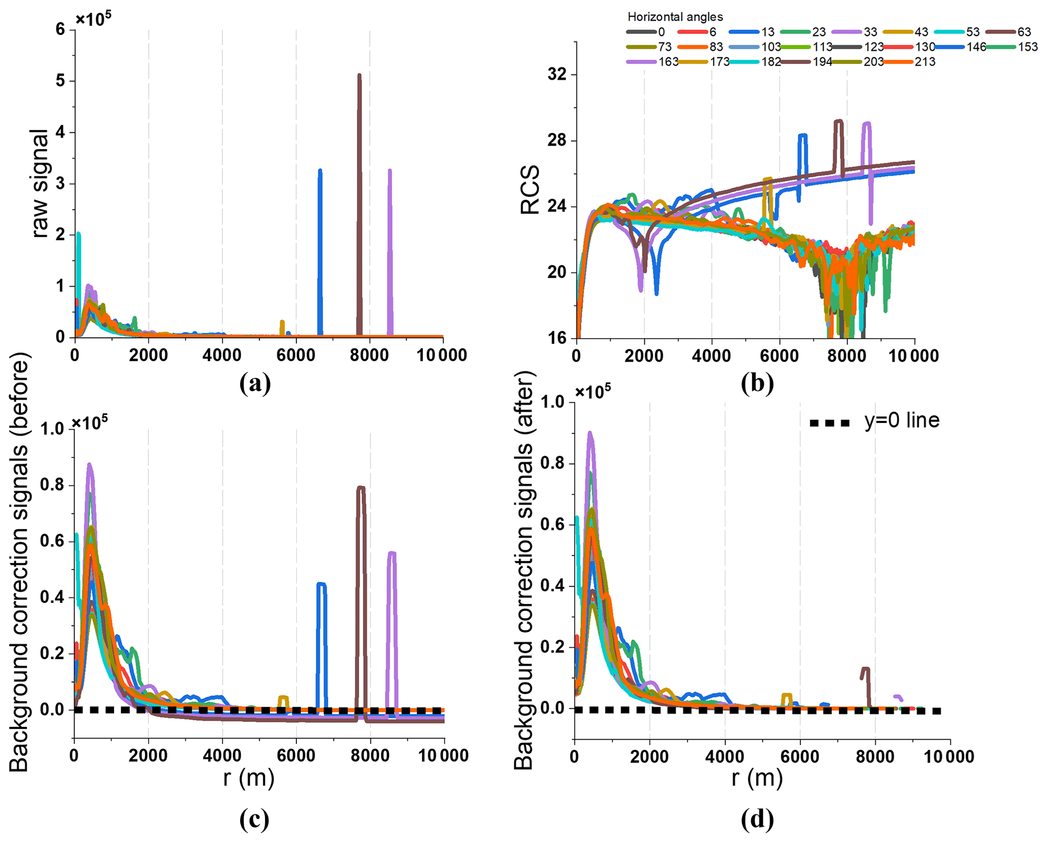
Figure 1 Steps of the improved background correction at 1064 nm for measurement at 13:17 local time on 23 March 2022: (a) raw lidar signal, (b) range-corrected signal, (c) background-corrected signal with the common method, and (d) background-corrected signal with the improved method. Colour refers to profiles related to different scan angles.

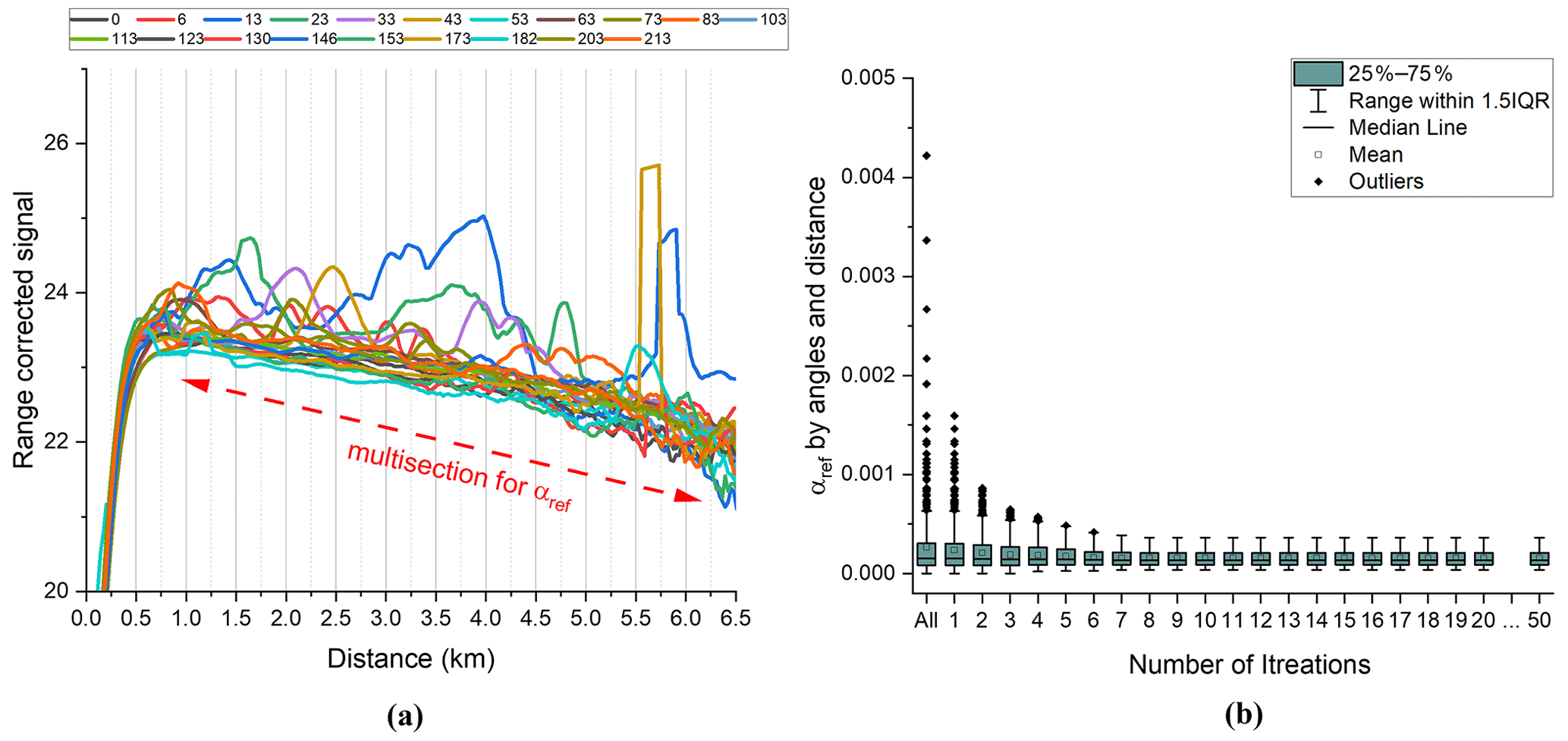
Figure 2 The 1064 nm range-corrected signal from measurements at 13:17 local time on 23 March 2022 (a) and the spread of inferred α_ref over 50 iterations (b).

2.2 Extinction coefficient retrieval

The elastic lidar equation at a single wavelength λ (Fernald et al., 1972; Klett, 1985) can be expressed as

$$\begin{array}{}\text{(1)}& P\left(r\right)=P_{\mathrm{0}}{\displaystyle \frac{c\mathit{\tau }}{\mathrm{2}}}A{\displaystyle \frac{\mathit{\beta }\left(r\right)}{r^{\mathrm{2}}}}\exp \left[-\mathrm{2}\underset{\mathrm{0}}{\overset{r}{\int }}\mathit{\alpha }\left(r^{\prime }\right)\mathrm{d}{r}^{\prime }\right],\end{array}$$

where P(r) is the power received from the range r, P₀ is the intensity of the emitted light at time t₀, α(r) is the extinction coefficient, β(r) is the backscatter coefficient, c is the speed of light, τ is the laser pulse duration, and A is the area of the receiver telescope. The factor $c\mathit{\tau }/\mathrm{2}A$ is the instrument constant (Klett, 1981).

The Klett–Fernald inversion estimates an initial extinction coefficient using the slope method (Fernald et al., 1972; Klett, 1981). To calculate the aerosol extinction coefficient, the reference extinction coefficient (α_ref) at the reference distance r_ref is substituted into the Klett equation (Klett, 1985) equation:

$$\begin{array}{}\text{(2)}& \mathit{\alpha }\left(r\right)={\displaystyle \frac{\exp \left[\frac{S\left(r\right)-S_{\mathrm{ref}}}{k}\right]}{{\mathit{\alpha }}_{\mathrm{ref}}^{-\mathrm{1}}+\frac{\mathrm{2}}{k}{\int }_r^{r_{\mathrm{ref}}}\exp \left[\frac{S\left(r\right)-S_{\mathrm{ref}}}{k}\right]\mathrm{d}{r}^{\prime }}}.\end{array}$$

Here, S(r)=ln[P(r)r²] contains the range-corrected signal P(r)r², while k depends on the characteristics of the measured aerosols and usually varies between 0.67 and 1.0 (Curcio and Knestrick, 1958).

Before the extinction coefficient retrieval, the distance resolution is decreased from 4.8 to 28.8 m by summing up six range bins. Then, a background correction based on the signal-to-noise ratio, calculated as the average of 150 data points at the far end of the measurement range, is applied. Finally, signals are further smoothed with a moving average using a window length of 180 m. This pre-processing ideally reduces or eliminates signal fluctuations. After successful retrieval, the inferred aerosol extinction coefficient is visualized through mapping.

Our horizontally scanning lidar observations are typically conducted at low altitudes of about 10 m above ground. Hence, finding suitable r_ref and α_ref form a major part of the analysis. This process is described in the next section.

2.3 Improved analysis of horizontal scans

We make two assumptions for inferring the horizontal aerosol distribution for scanning lidar measurements at different azimuth angles. First, aerosol is distributed homogeneously over the scanned area, i.e. in all directions, if there are no emission sources. While aerosol concentration generally decreases with height, similar aerosol concentration and a negligible molecular contribution can be expected in a horizontal plane. Second, as any point in the scanned area could be an emission source, it is more likely that the reference distance for the Fernald–Klett inversion is a function of scan angles. The latter complicated the analysis as horizontal measurements are often performed to identify emission sources and track their related aerosol plumes.

Figure 3 Data processing flowchart of the multi-section method.

Here, we propose a method for stable and spatio-temporally consistent solutions of the Fernald–Klett inversion, even in heterogeneous aerosol conditions. The new method consists of two steps: the background noise correction and the identification of r_ref and α_ref for application to a full planar scan. The first step screens the data for abnormal signals at larger distances from the instrument. Previous research suggests background correction based on equidistant designation (Cao et al., 2013; Manninen et al., 2016), but these methods are optimized for vertically pointing lidar observations. To remove unreasonable peaks and noise from the horizontal measurements at distances where we would expect to see background values, i.e. towards the end of a profile, we exclude outliers that exceed 3σ (Hodge and Austin, 2004) and added a model-fitting process based on Eq. (3),

$$\begin{array}{}\text{(3)}& y=a{e}^{bx}+c,\end{array}$$

which is an exponential function based on the lidar equation except for data in the near range. Here, x and y represent the measurement distance and the lidar signal, respectively, while a, b, and c are constant as calculated through model fitting as the primary background value. We compare c to the average signal in the background range and pick the lower of the two values as background noise.

The steps of the improved background correction are shown in Fig. 1. Abnormal peaks between 6 and 9 km distance are visible in the 1064 nm raw lidar signal for scan angles of 146, 163, and 194^∘. Such peaks can occur in any measurement and might be the result of scattered sunlight or temporary optical path obstruction by moving objects. If included in the background correction, these individual peaks are strong enough to move the background-corrected signal to negative values (Fig. 1c) and to inhibit the calculation of a range-corrected signal (Fig. 1b). The new methods lead to positive background-corrected signals (Fig. 1d) that allow for calculating a range-corrected signal.

The second part of the improved method is related to identifying the reference distance for the Fernald–Klett inversion. The reference value α_ref is derived as the distance slope of the logarithmic range-corrected signals as calculated after the new background correction. The reference distance is the range at which the retrieved aerosol backscatter coefficient equals α_ref. If set correctly, the inferred extinction coefficient decreases with distance, except for ranges at which aerosols are present (Mattis et al., 2008). The solution becomes unstable if r_ref is set incorrectly. In the case of near-zenith measurements, r_ref is usually set to somewhere between 5 and 10 km, which refers to the free troposphere where aerosol load is generally low or negligible. Following this approach, we initially set r_ref=5 km. However, this fixed value cannot be universally applied in horizontal measurements. Instead, r_ref and α_ref have to be set to regions where aerosol is relatively homogeneously distributed.

The steps for identifying α_ref are illustrated in Fig. 2. At each scan angle, we consider 21 reference points for calculating α_ref starting at 1 km distance in intervals of 250 m and refer to the result as multi-section α_ref (Fig. 2a). The total number of inferred values of α_ref is 21 times the number of scan angles (22 from 0 to 207^∘ in this study). To converge in α_ref we iteratively remove outliers from the average slope calculation if they exceed 1 standard deviation σ. Routinely, 50 iterations are performed, but most outliers are already removed after 10 iterations (Fig. 2b). Finally, the realistic α_ref is used in the Fernald–Klett inversion with r_ref=5 km.

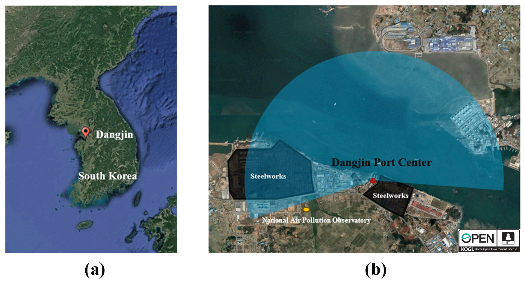
Figure 4 (a) Location of the scanning lidar at Dangjin Port Center, South Korea (© Google Earth 2023), and (b) the scanned area with the locations of industrial sites. The yellow dot designates the position of a site within the national air quality monitoring network. The map image is used under the Korea Open Government License (KOGL).

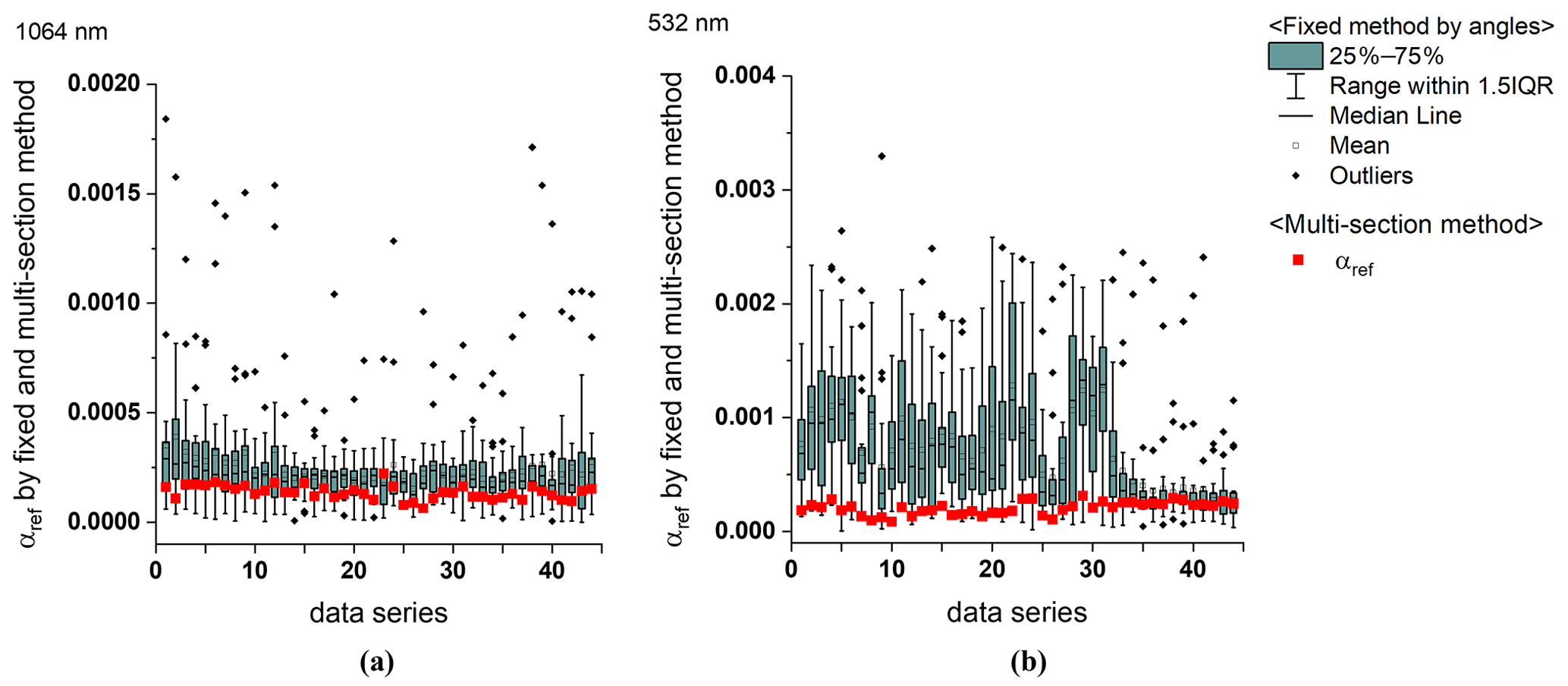
Figure 5 Temporal change in α_ref as inferred using the conventional fixed method (grey bars) and the new multi-section method (red) from scanning lidar measurements at 1064 (a) and 532 nm (b) for 45 planar scans between 09:17 and 20:53 on 23 March 2022.

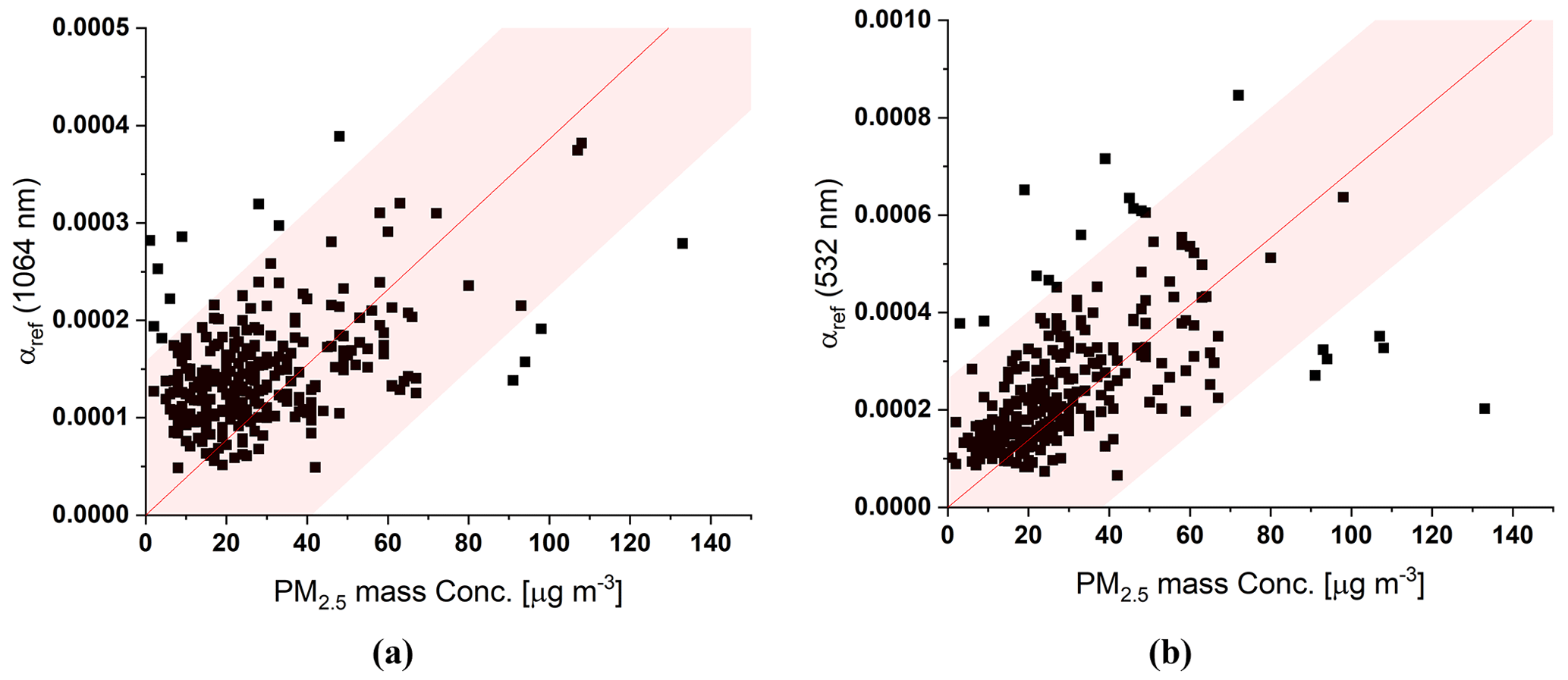
Figure 6 Comparison of α_ref as inferred by the multi-section method at 1064 nm (a) and 532 nm (b) at measures between 20 February and 29 March 2022 with PM_2.5 mass concentrations at a measurement site of the national observatory of the Korean Ministry of Environment. The linear regression is shown as a dashed line, while the coloured area indicates the 95 % prediction band.

The distinctive feature of this method is that the α_ref in the multi-section area replaces the value at 5 km, where the farthest distance has reliable signals. Therefore, the reference distance assumes all stable points without emissions or noise rather than pinpointing any specific point within the analysis area. Substituting the 5 km value with the α_ref obtained iteratively when calculating using the Klett inversion method implies that we can calculate the reliable extinction coefficient, even if there was noise in the long-range region.

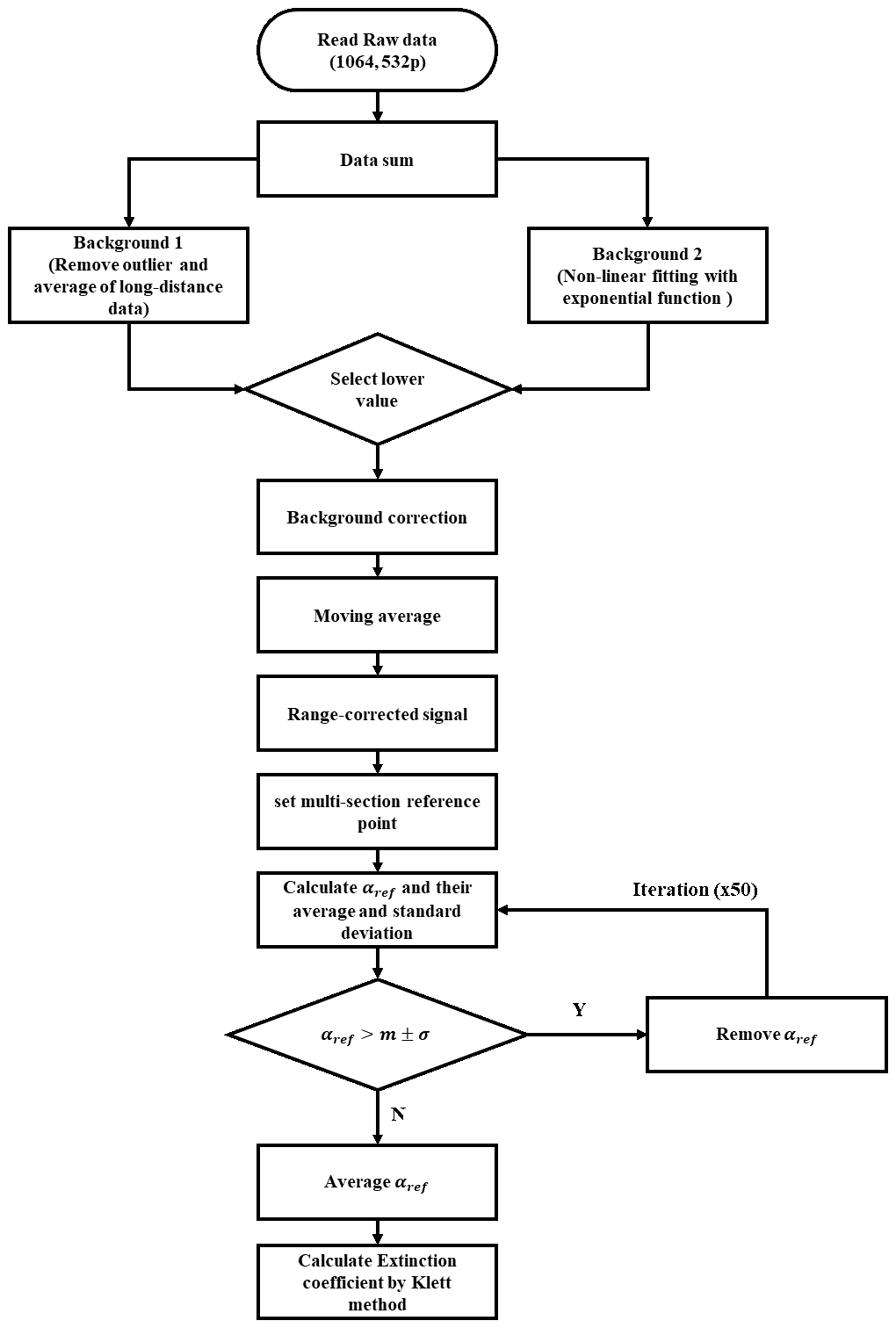
We refer to the new algorithm to calculate the extinction coefficient from horizontally scanning lidar measurements based on the Fernald–Klett method as the multi-section method. An overview of the different steps of the data processing is presented in Fig. 3.

2.4 Study area

The scanning lidar system was installed on the roof of Dangjin Port Center (36^∘59^′07.7^′′ N, 126^∘44^′44.2^′′ E) to scan the Anseom port area (Godae-ri, Songak-eup, Dangjin-si Chungcheongnam-do, Republic of Korea). Dangjin has a developed steel industry, and many steelworks exist in the Seokmun National Industrial Complex. In addition, there are various large-scale industrial complexes, such as Bugok Industrial Complex and Songsan Commercial Complex. The location of the site and the scanned area are illustrated in Fig. 4.

3 Results and discussion

The multi-section method allows for retrieving values of α_ref in areas of homogeneous aerosol conditions that are consistent within individual scans. As these values are assumed to refer to ambient background conditions, it is expected that there is little variation between subsequent scans with 10 to 15 min distance.

Figure 5 shows that the fixed method, i.e. rigidly selecting α_ref at 5 km distance for each scan angle individually, leads to a large spread of values for single scan and between scans. Some of those values cannot be used to produce stable solutions of the Fernald–Klett inversion. In contrast, the multi-section method produces reference values that represent the entire scan and are also consistent between time steps. These results allow for always obtaining stable solutions of the Fernald–Klett inversion and, thus, an automated quantitative analysis of the measurements.

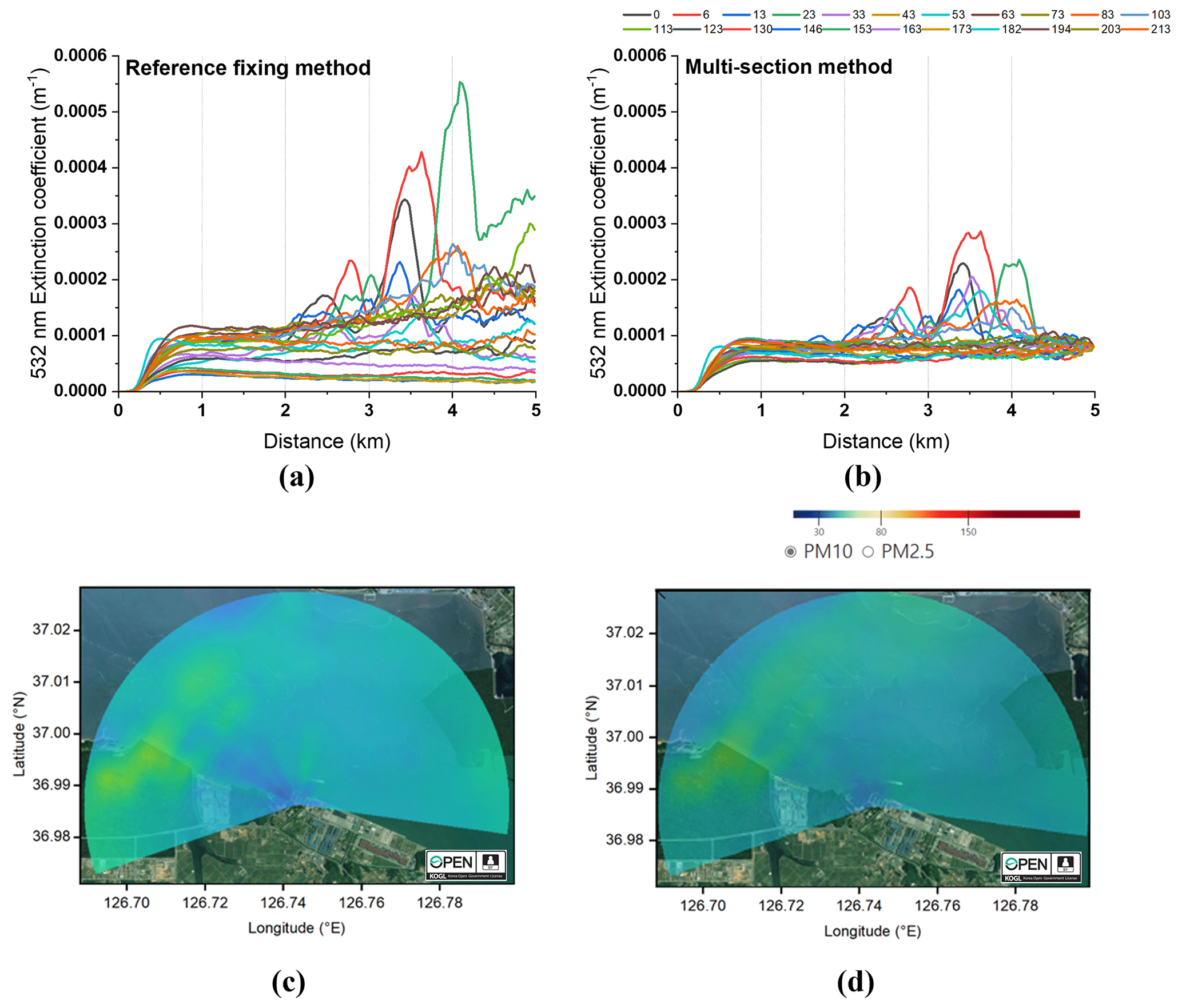
Figure 7 Angular resolved extinction coefficient at 532 nm (a, b) and inferred PM₁₀ concentration (c, d) as obtained by using the fixed reference value method (a, c) and the multi-section method (b, d) from a lidar scan at 20:14 local time at 27 February 2022. Coloured lines in the upper panels refer to different scan angles while the shading in the lower panels marks PM₁₀ concentration. The map image is used from KOGL.

Aerosol extinction is a measure of aerosol load. As α_ref represents aerosol concentrations at homogeneous background conditions, one can expect it to correlate with other measures of aerosol load such as PM_2.5 mass concentrations. Such measurements are performed at the national air quality monitoring sites of the Korean Ministry of Environment. To verify the results of the multi-section method, inferred α_ref is compared to PM_2.5 mass concentrations measured at a site about 2.8 km away from the lidar's scan area (see Fig. 4). Figure 6 presents a high correlation (r²=0.77) between α_ref at 532 nm and PM_2.5 mass concentrations, with most points within the 95 % prediction band. Outliers are likely related to the different time resolutions of the measurements, with lidar data available in intervals of about 15 min and in situ mass concentrations given as hourly averages. In contrast to the lidar measurements at 532 nm, α_ref at 1064 nm is less correlated to PM_2.5 concentration (r²=0.74) and also shows a broader 95 % prediction band. While the different temporal resolution is likely to affect the comparison at 1064 nm as well, it is well known from light-scattering theory that longer lidar wavelengths are less sensitive to fine particles.

For the purpose of monitoring air quality, the aerosol extinction coefficients inferred from our scanning lidar measurements are converted to PM_2.5 and PM₁₀ mass concentrations using the wavelength-dependent Ångström exponent, lidar ratio, and aerosol extinction efficiency, as mentioned in Sect. 2.1 (Liu et al., 2020; Noh et al., 2008, 2020). The lidar-derived PM mass distribution is interpolated by primary linear regression fitting for visualization.

The impact of the improved method for the analysis of scanning lidar measurements on the retrieved aerosol extinction coefficient and the subsequently inferred PM₁₀ mass concentration is presented in Fig. 7. The use of a reference value derived at 5 km distance for different scan angles causes a strong overestimation of extinction coefficient maxima as it is strongly affected by signal noise at that distance. At the same time, individual profiles differ strongly in their baseline values. This is visible by a large spread in the profiles in Fig. 7a. The spread is reduced to a consistent and stable background when the multi-section method is applied. As a result, the PM₁₀ field inferred from the multi-section analysis of the scanned plane is more homogeneous than the one obtained using the traditional method. It no longer contains exaggerated emission sources, increased values at the fringes of the covered area, or artificial features in the vicinity of the lidar. Consequently, the new analysis method is found to be very valuable for reliably and automatically obtaining secondary products for environmental monitoring.

4 Conclusions

We have developed a horizontally scanning lidar for monitoring the spatio-temporal distribution of aerosol concentrations. The observations are used to obtain aerosol extinction coefficients as a function of scan angle, wavelength, and distance. To overcome difficulties in the application of the Fernald–Klett method to horizontal measurements, we have developed a novel method for inferring the reference extinction coefficient. The new multi-section method first reduces background noise by dismissing signal peaks that exceed 3σ of the mean over individual scans of each angle. After the noise correction, an iterative approach is used for identifying a value of α_ref that is stable within full-scan measurements and is, thus, likely to represent ambient background conditions. A comparison of lidar-inferred aerosol mass concentrations to independently measured PM_2.5 mass concentrations at Korean air quality monitoring sites confirms that α_ref can represent the concentration of ambient aerosols. The r² values of PM_2.5 mass concentration with α_ref at 1064 and 532 nm were 0.74 and 0.77, respectively. The application of the new method leads to a consistent picture of extinction coefficients and aerosol concentrations throughout the scanned area. These improvements related to the new analysis method emphasize the applicability of horizontally scanning aerosol lidar measurements for quantitative source identification and air quality monitoring.