the Creative Commons Attribution 4.0 License.
the Creative Commons Attribution 4.0 License.
 | 08 Jul 2024
Regional validation of the solar irradiance tool SolaRes in clear-sky conditions, with a focus on the aerosol module
Thierry Elias
Nicolas Ferlay
Gabriel Chesnoiu
Isabelle Chiapello
Mustapha Moulana
The Solar Resource estimate (SolaRes) tool based on the Speed-up Monte Carlo Advanced Radiative Transfer code using GPU (SMART-G) has the ambition to fulfil both research and industrial applications by providing accurate, precise, and high-time-resolution simulations of the solar resource. We investigate the capacity of SolaRes to reproduce the radiation field, relying on 2 years of ground-based measurements by pyrheliometers and pyranometers acquired in northern France (Lille and Palaiseau). Our main objective is to provide, as a first step in clear-sky conditions, a thorough regional validation of SolaRes, allowing us to investigate aerosol impacts on solar resource. We perform comparisons between SolaRes-simulated and clear-sky-measured global horizontal irradiance (GHI), direct normal irradiance (DNI), diffuse horizontal irradiance (DifHI), and global and diffuse irradiance on a tilted plane (GTI, DifTI), and we even consider the circumsolar contributions.
Using spectral aerosol optical thickness (AOT) data sets as input, which are delivered by the AErosol RObotic NETwork (AERONET) and the Copernicus Atmosphere Monitoring Service (CAMS), we examine the influence of aerosol input data sets in SolaRes on the comparison scores. Two aerosol models are mixed to compute aerosol optical properties. We also perform a sensitivity study on the aerosol parametrisation and investigate the influence of applying more or less strict cloud-screening methods to derive ground-based proof data sets of clear-sky moments.
SolaRes is validated with the (relative) root mean square difference (RMSD) in GHI as low as 1 % and a negligible mean bias difference (MBD). The impact of the cloud-screening method in GHI is 0.5 % of RMSD and 0.3 % of MBD. SolaRes also estimates the circumsolar contribution, which improves MBD in DNI and DifHI by 1 % and 4 %, respectively, and RMSD by ∼ 0.5 %. MBD in DNI is around −1 % and RMSD around 2 %, and MBD in DifHI is 2 % and RMSD around 9 %. RMSD and MBD in both DNI and DifHI are larger than in GHI because they are more sensitive to the aerosol and surface properties. DifTI measured on a vertical plane facing south is simulated by SolaRes with an RMSD of 8 %, comparable to that obtained for DifHI. Our results suggest a strong influence of reflection by not only ground surface but also surrounding buildings.
The sensitivity studies on the aerosol parameterisation show that the spectral AOT contains enough information for high performance in DNI simulations, with low influence of the choice of the aerosol models on the RMSD. However, choosing a model with smaller aerosol single scattering albedo significantly decreases SolaRes DifHI and GHI. The best combination in Lille and Palaiseau consists of continental clean mixed with desert dust. Also, complementary information on angular scattering and aerosol absorption provided by the AERONET-inverted model further improves simulated clear-sky GHI by reducing RMSD by ∼ 0.5 % and MBD by ∼ 0.8 %. Eventually, the choice of the data source has a significant influence. Indeed, using CAMS AOT instead of AERONET AOT increases the RMSD in GHI by ∼ 1 % and MBD by ∼ 0.4 % and RMSD in DNI by 5 %. The RMSD in GHI remains slightly smaller than state-of-the-art methods.
- Article
(1276 KB) - Full-text XML
- BibTeX
- EndNote


Incident solar radiation on collecting systems is one of the main influencing parameters of the electrical productivity by a solar plant. Incident solar radiation is highly variable in time and space because of changing atmospheric optical properties affected by clouds, aerosols, water vapour, and ozone, as well as surface reflection and solar direction geometry. The electricity production also depends on the panel orientation and inclination relative to the incident solar radiation direction and on its spectral absorption efficiency.
The aim of the Solar Resource estimate (SolaRes) tool is to provide precise and accurate simulations of the solar resource at 1 min resolution for any location on the globe, in any meteorological and ground surface conditions and for any solar plant technology. SolaRes consequently suits many applications from research to industrial fields. SolaRes is powered by the Speed-up Monte Carlo Advanced Radiative Transfer code using GPU (SMART-G), which physically resolves the radiative transfer equation (Ramon et al., 2019). Until now, physical radiative transfer codes have rarely been used to estimate the solar resource for industrial needs in solar energy (e.g. Sun et al., 2019) as they are usually slower than approaches based on abaci or look-up tables. However, the particular design of SMART-G makes it a suitable tool for such endeavours, as computations are hastened through a parallelisation approach on GPU cards. The use of a physical radiative transfer code offers the advantage of precision and accuracy, as well as flexibility.
SMART-G could be ranked in the class A (physical radiative transfer code) classification defined by Gueymard and Ruiz-Arias (2015), as any angular and spectral characteristics of the solar radiation field can be computed on demand. This possibility is particularly important for photovoltaic (PV) applications as, according to Lindsay et al. (2020), computation of spectrally and angularly refined irradiances could decrease the error in simulated electrical power produced by the photovoltaic set-up by up to 15 %. This is the reason for using a code such as SMART-G in SolaRes. SMART-G is able to compute interactions between solar radiations and the atmosphere in a 3D environment but is run in the plane-parallel homogeneous-layer mode for this paper.
SolaRes and its regional validation are described in this paper. SolaRes provides not only the global horizontal irradiance (GHI) as the standard solar resource component, but also other components depending on the angular behaviour of the radiation field, such as the direct normal irradiance (DNI) and the diffuse horizontal irradiance (DifHI), as well as the projected quantities on a tilted plane, i.e. the global tilted irradiance (GTI) and the diffuse tilted irradiance (DifTI). Such components are essential for describing processes involved in solar technologies and also related to vegetation (e.g. Mercado et al., 2009). Note that SolaRes encompasses the Attenuation of the Solar Radiation by Aerosols (ASoRA) method for DNI estimates, which has been validated in clear-sky conditions in an arid environment (Elias et al., 2021). SolaRes allows for computations of circumsolar contribution, and it provides two estimates of direct normal irradiance (DNI): (1) DNIpyr, consistent with observed DNI, which includes circumsolar contribution, and (2) DNIstrict, not including circumsolar contribution but consistent with computations of solar resource parameters in any panel orientation. Usually, physical or semi-physical models provide only one of these two estimates of DNI. For example, Gueymard and Ruiz-Arias (2015) remind us that circumsolar contribution is not considered by any of the 24 models they have selected for their review.
As computation uncertainties come from both the model and the input data set, the validation must be performed with an input data set defined with the best precision. Aerosol optical thickness (AOT) can be measured at local scale with high precision by the ground-based photometers of the AErosol RObotic NETwork (AERONET) (Holben et al., 1998). In addition, aerosol layers can be approximated as being located in a plane-parallel homogenous layer, which is consistent with the SMART-G mode in SolaRes. On the contrary, cloud optical thickness can not be inferred with such a high precision at the local scale, and cloudy atmospheres have complex structures, rarely close to plane-parallel homogenous layers. The regional validation is thus performed in the absence of clouds, i.e. under clear-sky conditions, for which the variability of the solar radiation mainly relates to the influence of aerosols and solar geometry.
A major process thus consists of identifying the clear-sky moments in a region north of France, characterised by highly variable overcast conditions. Many methods have been defined in the literature. Based on the review of Gueymard et al. (2019), we select and adapt two methods presenting contrasting results in terms of representativity of the atmospheric variability, which allow us to assess the influence of cloud-screening methods on the evaluation of SolaRes simulations. The first method, based on García et al. (2014), accounts for daily AOT variability and is thus quite representative of the site's typical clear-sky atmospheric conditions; however it misses some cloudy conditions. The second cloud-screening method, based on Long and Ackerman (2000), does not account for changes in AOT and thus tends to eliminate clear-sky situations characterised by high aerosol loads.
The field of solar energy research benefits from other research areas, such as climate studies. Indeed, some of the measurements of solar radiation used here as ground-based proof for validation were acquired by the Baseline Surface Radiation Network (BSRN) (Driemel et al., 2018), whose first mission was to monitor components of the Earth's radiative budget and their changes over time, especially in response to the “increasing debate on anthropogenic influences on climate processes during the 1980s” (Driemel et al., 2018). In the same field, AERONET contributes to the estimate of global aerosol radiative forcing by validating aerosol satellite remote sensing retrievals and also aerosol climate models, in the context of global greenhouse warming. This paper thus presents a radiative closure study. Indeed, two categories of independent, simultaneously co-located measurements can be connected by a radiative transfer code (e.g. Michalsky et al., 2006; Ruiz-Arias et al., 2013). The regional validation is performed on data sets acquired in Lille and Palaiseau in 2018–2019, both located in northern France.
From a radiation perspective, one of the main impacts of aerosols is to extinguish the direct component of the incident solar radiation at surface level. Spectral AOT consequently efficiently constrains DNI (Elias et al., 2019, 2021). Spectral AOT also partly describes the aerosol scattering properties which significantly affect DifHI. However some information on aerosol absorption and surface reflection is missing. Sensitivity studies are performed to show the efficiency and the limits of the current version of the SolaRes tool.
Section 2 describes the observational and modelling data sets used as input to SolaRes, as well as the solar irradiance measurements used as ground-based proof for validation. Section 3 briefly describes SMART-G and the parameterisations used in SolaRes, especially those related to the aerosol optical properties. Section 4 presents two cloud-screening procedures and investigates their impact on the validation data set and on the factors affecting radiative transfer such as AOT. Section 5 presents the results of the comparison performed between SolaRes estimates and solar irradiance ground-based measurements. Thereafter, Sect. 6 shows the sensitivity of the comparison scores to the aerosol parameterisation, considering two main influences: (1) the hypothesis on the mean aerosol nature and (2) the aerosol data source. Indeed, the Copernicus Atmosphere Monitoring Service (CAMS), which assimilates satellite data sets to describe air quality on a global scale, is also used here as an input data provider.
Our analysis of SolaRes performances relies on different types of data. SolaRes requires input data provided either by a ground-based instrumentation network (Sect. 2.3) or by a global atmospheric model (Sect. 2.4). The solar resource components simulated by SolaRes (Sect. 3) are validated (Sect. 5) by comparisons with ground-based measurements (Sect. 2.2).
2.1 Choice of the two sites
Two platforms located in the northern part of France are chosen, both embedded in a sub-urban environment and both hosting a comprehensive set of radiative instruments. This choice is motivated by several arguments.
First, downwelling solar irradiance is measured at surface level with a distinction between direct and diffuse components, at both sites. Measurements in Palaiseau (France; 48.7116° N, 2.215° E; 156 m a.s.l.) contribute to the Baseline Surface Radiation Network (BSRN) (Driemel et al., 2018), which brings a high source of confidence. Measurements at the ATmospheric Observations in LiLLe (ATOLL) platform (France; 50.61167° N, 3.141670° E; 60 m a.s.l.) are also of high quality, confidently known by the authors, and the site in addition provides interesting solar irradiance measurements on tilted planes that are exploited in Sect. 5.4.
Secondly, the two sites provide accurate measurements of aerosol loading as they are AERONET sites. Third, the aerosol loading above these two sites is quite representative of observations over western Europe. While not at the level of high loading due to natural aerosol (e.g. desert dust) or strong anthropogenic emissions (e.g. some areas in China or India), the observed aerosol loading is moderate by European standards. The aerosol loadings are quite variable and diverse, resulting from changing meteorology: a relatively clean influence from the ocean, often occurring in winter, and a continental influence due to the transport of anthropogenic pollution from road traffic and agriculture, which is particularly important during anticyclonic situations in spring. According to the Köppen–Geiger climate classification (Beck et al., 2018), both sites are affected by a climate similar to that of western Germany (Witthuhn et al., 2021), England, Ireland, Belgium, and the Netherlands, which is labelled Cfb.
The last arguments to retain these sites is that cloudy situations are numerous. Therefore, these two sites are appropriate to test cloud-screening techniques, particularly those that do not falsely reject clear-sky conditions with loads other than pristine conditions.
2.2 Ground-based irradiance measurements used as a validation data set
2.2.1 The ATOLL platform
Since 2008, a set of class A Kipp & Zonen instruments mounted on an EKO sun tracker (STR-22) has been routinely measuring the solar downward irradiance at the ATmospheric Observations in LiLLe (ATOLL) platform (France; 50.61167° N, 3.141670° E; 60 m a.s.l.) on the Lille University campus (https://www-loa.univ-lille1.fr/observations/plateformes.html?p=lille, last access: 7 April 2023; the site is named Lille in the paper). A CHP1 pyrheliometer (Kipp & Zonen, 2008) measures the direct normal irradiance (DNIobs) in a field of view of 5 ± 0.2°. A CMP22 pyranometer (Kipp & Zonen, 2013) associated with a shadowing ball measures the diffuse horizontal irradiance (DifHIobs). Both DNIobs and DifHIobs are provided at 1 min resolution.
Calibrations performed in 2012, 2017, and 2022 show a relative stability of the instrument performances. Indeed, the CHP1 calibration coefficient varies by a maximum of 3 % over the period, and the CMP22 calibration coefficient decreases by less than 1 %. According to Witthuhn et al. (2021), the uncertainty under clear-sky conditions is 2 % for GHI, 4 % for DifHI because of the shadowing device, and 5 % for DNI. Winter gaps of a few weeks exist in the data time series when the instruments were sent either to Delft (the Netherlands) for a recalibration (by Kipp & Zonen) or to M'Bour (Senegal) to be used as a reference for the calibration of local instruments.
Observed global horizontal irradiance (GHIobs) in Lille is obtained as the sum of direct and diffuse components, which is the preferred method for the measurement of global irradiance (Flowers and Maxwell, 1986). This method avoids most cosine response errors in the instrument at low-sun angles (Michalsky and Harrison, 1995; Mol et al., 2024) and results in smaller uncertainties in GHIobs compared with unshaded instruments (Michalsky et al., 1999). The summation is indeed chosen by BSRN (Ohmura et al., 1998) and can be expressed as
with
where μ0=cos (SZA), and SZA is the solar zenith angle.
Additionally, since 2017, the ATOLL platform has also hosted an unshaded class A Kipp & Zonen CMP11 pyranometer, which measures the global tilted irradiance (GTIobs) for various inclinations. Both the CHP1 and the CMP22 instruments measure radiation in the broadband range between 210 and 3600 nm, while the spectral range for the CMP11 pyranometer extends between 270 and 3000 nm.
Note that the CMP11 is set horizontally in the spring–summer of 2018 for an intercomparison campaign with both CHP1 and CMP22. Comparison is made during clear-sky minutes found over 47 d (according to the Garcia cloud-screening method presented in Sect. 4). The mean relative difference between GHIobs measured by the CMP11 and CHP1 + CMP22 instruments is found to be −8 ± 5 W m−2 (1.6 ± 0.9 %) (with CMP11 providing smaller values than CHP1 + CMP22), and the root mean square difference (RMSD) is 9 W m−2 (1.9 %), which is within the instrumental uncertainties.
Our analysis focuses on the 2018–2019 time period, which is close to the 2017 calibration and includes the intercomparison campaign of 2018, and the time period with vertical CMP11 in 2019, which allows for validation of SolaRes under different angular configurations.
2.2.2 BSRN site of Palaiseau
Solar resource measurements are made in Palaiseau (France; 48.7116° N, 2.215° E) as part of BSRN by three Kipp & Zonen CHP1 and CMP22 instruments, similar to those running in Lille. GHIobs and DNIobs are measured by CMP22 and CHP1, respectively, and DifHIobs is measured by a second CMP22 mounted with a sun-tracking shadower device. A 1 Hz sampling rate is recommended for radiation monitoring, and measurements are recorded and provided at 1 min time resolution. Uncertainty requirements for the 1 min BSRN data are 5 W m−2 for DifHIobs and 2 W m−2 for DNIobs (Ohmura et al., 1998).
2.3 AERONET provides input data sets on aerosols and water vapour
Coincidentally with the irradiance measurements, AERONET photometers (Holben et al., 1998) acquire data at both Lille and Palaiseau. We use direct measurements of aerosol optical thickness (AOT) at both 440 and 870 nm, as well as the column water vapour content (WVC), as input to the SolaRes algorithm. We use Level 2.0 data quality, applying a clear-sun screening procedure, and version 3 of AERONET data (Sinyuk et al., 2020), which also provides ozone content from the Total Ozone Mapping Spectrometer (TOMS) monthly average climatology (1978–2004). The expected uncertainty in AOT is 0.01–0.02 at these wavelengths (Dubovik et al., 2000; Giles et al., 2019). AOT measurements are made at a sampling rate of around 3 min (Giles et al., 2019) in clear-sun conditions.
In addition to AOT measurements at several wavelengths, AERONET provides inverted aerosol models at around 1 h resolution, which are composed of the phase function and the aerosol single scattering albedo at several wavelengths. Due to the sparsity of the Level 2.0 inverted data set, which limits the statistical significance of our assessment, we chose to use Level 1.5 inversion data, similar to other authors (Ruiz-Arias et al., 2013; Chen et al., 2021; Witthuhn et al., 2021), despite the probable larger uncertainties. Ruiz-Arias et al. (2013) mention an increase in the uncertainty in Level 1.5 (V2) aerosol single scattering albedo (SSA) compared to Level 2.0 in the 0.05–0.07 range, while Witthuhn et al. (2021) mention an uncertainty of 0.03 for Level 1.5, consistently with an uncertainty of ±0.03 for v3 Level 2.0 by Sinyuk et al. (2020). The “hybrid scan” option (Sinyuk et al., 2020) is chosen. AOT at 3 min is chosen to generate the SolaRes input data for validation (Sect. 5), and the 1 h AERONET-inverted aerosol models are used for a sensitivity study (Sect. 6.2).
2.4 CAMS provides input data sets for aerosols, water vapour, and surface albedo
Data from the Copernicus Atmosphere Monitoring System (CAMS) (Benedetti et al., 2009; Morcrette et al., 2009) are used to investigate the sensitivity of SolaRes to the aerosol data source (Sect. 6.3). To be consistent with an operational near-real-time (NRT) service, the CAMS-NRT data set is used. AOT at several wavelengths, as well as WVC, and ozone content are provided by CAMS-NRT. The spatial resolution is 0.4°, and the time resolution is 1 h. For this paper, global CAMS-NRT data sets were downloaded from the Copernicus Climate Data Store (https://ads.atmosphere.copernicus.eu/cdsapp/#!/dataset/cams-global-atmospheric-composition-forecasts?tab=form, last access: 27 August 2022). CAMS-NRT AOT at 469 and 865 nm is used to compute the Ångström exponent α (indicator of the spectral dependence of AOT), which allows us to infer AOT at both 440 and 870 nm (see for example Witthuhn et al., 2021), used as input by the SolaRes algorithm (see Sect. 3.3.2). The Ångström exponent is expressed as
where λ1 and λ2 are two wavelengths. The comparison with AERONET direct measurements gives an RMSD of ∼ 50 % in AOT (0.10 at 440 nm and 0.04 at 870 nm) and 25 % (0.3) for α. The MBD is smaller than 5 % in both AOT and α. These comparison results are similar to those of Witthuhn et al. (2021) and the references therein, over Germany for the CAMS reanalysis data set.
CAMS-NRT data time series in Lille and Palaiseau were also downloaded from the CAMS radiation service (https://www.soda-pro.com/web-services/radiation/cams-mcclear, last access: 15 March 2022). The “research mode” allows us to download not only GHI, DNI, and DifHI, but also the input data for the model, such as the solar broadband surface albedo, which is derived from the Moderate Resolution Imaging Spectroradiometer (MODIS), as described by Lefèvre et al. (2013). It is a combination of the white-sky and black-sky albedos, as a function of the proportion of the direct radiation in the global radiation (Lefèvre et al., 2013). Daily averages are computed, varying between 0.12 in November–December and 0.16 in June–July in Lille and Palaiseau, and are used as input in SolaRes radiative transfer simulations. A constant broadband surface albedo value of 0.2, which is a typical broadband value for grassland, is used by Lindsay et al. (2020), which is slightly larger than the values used here for Palaiseau.
Computations are made with the SolaRes v1.5.0 algorithm. SolaRes computes DNI according to the ASoRA method (Elias et al., 2021) and the diffuse irradiance with the SMART-G code (Ramon et al., 2019). The advantage of using SMART-G is to accurately compute the angular behaviour of the diffuse radiation field by considering aerosol and surface optical properties: the diffuse radiation can be computed for any inclination and orientation (DifHI and DifTI), and the circumsolar contribution can be estimated by computing the diffuse irradiance in a narrow field of view centred on the solar direction.
To better reproduce the solar resource time variability and to better evaluate the performances of SolaRes in clear-sky conditions, computations are made at a 1 min time resolution, as advised by several authors, such as Sun et al. (2019). On the one hand, DNI is computed at the time resolution of 1 min by interpolating aerosol optical thickness at 1 min. On the other hand, DifHI is computed at 15 min resolution by radiative transfer computations with SMART-G to limit the computational time and is then interpolated linearly at the 1 min resolution. GHI is computed by adding 1 min DNI projected on the horizontal plane (DirHI) and 1 min DifHI, as done by all high-performance models referenced by Sun et al. (2019), and a similarly method is used for GTI:
3.1 The direct contribution
3.1.1 DNIstrict and its projection
While DifHI and DifTI are computed with SMART-G (Sect. 3.2), DirHI and DirTI are computed by projecting DNI on a horizontal or tilted plane:
where ΩS is the unit vector in the solar direction:
where SAA is the solar azimuthal angle, and n is the unit vector perpendicular to the titled surface:
where i is the inclination of the titled surface and o its orientation, relative to the north and increasing eastward (as SAA). If the plane is horizontal, where i = 0 and , we get DirHI = DNI μ0 (Eq. 1b).
DNI can be either DNIstrict according to the “strict” definition given by Blanc et al. (2014) or DNIpyr, as observed by a pyrheliometer. For DNIstrict, only beams in the solar direction are counted, which are not scattered by the atmosphere. In other words, the circumsolar radiation is not accounted for. Underestimation of DNIobs by the DNIstrict method is thus expected. Consistently with the ASoRA method (Elias et al., 2021), DNIstrict is expressed as
FESD is the Earth–Sun distance-correcting factor. Spectral integration is made between the two wavelengths λinf and λsup. Esun(λ) corresponds to the extraterrestrial solar irradiance at the wavelength λ. Tcol(SZA,λ) represents the atmospheric column transmittance, which can be decomposed, under clear-sky conditions as follows:
where SZA is omitted for clarity. TRay(λ) is the transmittance caused by Rayleigh scattering along the atmospheric column, while Tgas(λ) is caused by absorbing gases, mainly water vapour and ozone in the solar spectrum. In clear-sky conditions, Tcol(λ) does not depend on the cloud transmittance. Taer(λ) is defined according to the Beer–Lambert–Bouguer law as
where mair is the optical air mass which can be approximated by and must take into account the Earth's sphericity for SZA above 80° (e.g. Kasten and Young, 1989).
3.1.2 Considering the circumsolar contribution
The pyrheliometer measures not only beams in the solar direction but also all scattered radiation within the instrument field of view. The difference between the observation and simulation is then expected to decrease by considering DNIpyr, defined as
where ΔDifNIcirc is the circumsolar contribution on a plane perpendicular to the solar direction. Moreover, the sun-tracking shadowing device, which allows a pyranometer to measure DifHI instead of GHI, blocks not only direct radiation but also radiation scattered around the sun. DifHIpyr is then defined as
where
3.2 Brief description of SMART-G
SMART-G allows us to simulate the propagation of polarised light (monochromatic or spectrally integrated) in a coupled atmosphere–ocean system in a plane-parallel or spherical-shell geometry, as described by Ramon et al. (2019). The code uses general-purpose computation on graphic processing unit technology (GPU) with other Monte Carlo variance reduction methods (local estimation, Marchuk et al., 1980; ALIS, Emde et al., 2011; etc.) to speed up the simulations while keeping high precision.
In this work SMART-G is used to simulate all diffuse irradiance parameters, i.e. DifHI, DifTI, and ΔDifNIcirc, in a plane-parallel atmosphere. DifHI is calculated by using the simple conventional method for planar flux in Monte Carlo radiative transfer codes, where the solar rays are tracked from the sun to the ground. The scattered rays reaching the ground surface are then counted to calculate DifHI. For DifTI we use a backward Monte Carlo tracking of solar radiation; i.e. the solar radiation rays are followed in the inverse path, from the instrument to the sun, with the local estimation method (Marchuk et al., 1980) to reduce the variance. The half-aperture angle is 90° to imitate the pyranometer. The circumsolar contribution, ΔDifNIcirc, is calculated similarly to DifTI but by assigning a half-aperture angle of 2.5° to imitate the pyrheliometer.
3.3 The radiative transfer parameterisation
3.3.1 Atmospheric gases and the surface
The extraterrestrial solar spectrum is taken from Kurucz (1992). Rayleigh optical thickness is computed according to Bodhaine et al. (1999) and scaled with the atmospheric pressure. The gas and thermodynamic profiles are adopted from the US summer standard atmosphere of the Air Force Geophysics Laboratory (Anderson et al., 1986), providing water vapour concentration profiles, scaled linearly with the columnar content of the input data. Ozone and NO2 absorption cross sections are taken from Bogumil et al. (2003), and we use the absorption band parameterisation provided by Kato et al. (1999) for other gases like H2O, CO2, and CH4. As UV-C radiation below 280 nm is absorbed by the atmosphere, spectral integration is made between 280 and 4000 nm for comparisons with CHP1 and CMP22 measurements and between 280 and 3000 nm for comparisons with CMP11 measurements. In k-distribution parametrisation, the bands between 280 and 4000 nm correspond to 30 spectral intervals with 297 Gaussian quadrature points named g points (Lacis and Oinas, 1991; Kato et al., 1999), and the bands between 280 and 3000 nm correspond to 28 spectral intervals with 267 g points. The surface is considered Lambertian, with a spectrally independent albedo.
3.3.2 Aerosol parameterisation
The measurements only partially describe the necessary input aerosol optical properties for radiative transfer computations. It is therefore compulsory to employ various strategies to get the necessary parameters from observation data sets. In SolaRes, similarly to the ASoRA method (Elias et al., 2021), we choose to mix two aerosol models, AM1 and AM2, which reproduce input AOT at two wavelengths:
where AOTinput(λ) is provided by AERONET or CAMS-NRT, and AOTAM1(λ) and AOTAM2(λ) are computed here from two aerosol models from the Optical Properties of Aerosols and Clouds (OPAC) database (Hess et al., 1998). To span a large range of Ångström exponent (α) values, it is recommended that one model is characterised by a large value of α and another by a smaller value of α. We then refer to a small-α model and a large-α model. λ1 and λ2 are 440 and 870 nm, respectively. The weights wAM1 and wAM2 are obtained from Eqs. (13a) and (13b) and are used to compute the aerosol transmittance at other wavelengths of the 280–4000 nm spectral interval. For the computation of the diffuse radiation components by SMART-G, the weights wAM1 and wAM2 are also applied to the aerosol phase function and single scattering albedo. A 3 min AOT is chosen to generate the SolaRes input data for the following reasons:
-
The main factor on GHI and DNI is AOT, which is proportional to the aerosol burden in the atmospheric column.
-
AOT is the usual aerosol information provided in both the observation and modelling data sets.
-
AOT is often provided at several wavelengths of the solar spectrum. Spectral AOT, or the Ångström exponent, is indicative of the aerosol size and consequently partly informs about the aerosol nature.
-
The 3 min resolution is adapted to follow any time evolution in the aerosol burden and nature. To reduce the computational burden and the number of radiative transfer computations, the AERONET data set is averaged at 15 min, and aerosol optical properties are generated at the resolution of 15 min to compute DifHI. The 15 min AOT is then interpolated at 1 min to compute 1 min DNI.
For the sensitivity study of Sect. 6.2, the AERONET-inverted aerosol model provides the aerosol phase function and single scattering albedo at the four wavelengths of 440, 675, 870, and 1020 nm (Sinyuk et al., 2020). In this case, AOT and the aerosol single scattering albedo (SSA) are linearly interpolated between 440 and 1020 nm; AOT is linearly extrapolated below 440 nm and above 1020 nm, while SSA remains constant; and the phase function at the closest wavelength is used. The vertical profile of AOT decreases exponentially with a vertical height of 2 km.
The validation is performed in clear-sky conditions when aerosols directly affect the surface solar irradiance but not the clouds. This section describes two cloud-screening methods relying on time series of solar irradiance measurements, selected based on the work of Gueymard et al. (2019), who compare the outputs of several cloud-screening algorithms to cloud cover observations by ground-based sky imagers for several locations in the US. The two methods are expected to show contrasting results in terms of comparison scores, as detailed in Sect. 5.
4.1 Choice of the cloud-screening procedure
Since the output of cloud-screening methods is binary, e.g. the sky is either cloudy or clear, Gueymard et al. (2019) evaluate the performances of the cloud-screening methods with a confusion matrix. As the aim of our study is to validate SolaRes simulations in clear-sky conditions, we need to select a cloud-screening method that maximises the number of correctly identified clear-sky cases or the true positive score (TPS). It is also important to keep the false positive score (FPS) as low as possible to avoid cases of incorrect identification and to minimise cloud contamination. The precision score (PS) may represent the performance of the screening method in identifying clear-sky moments:
Based on the TPSs and FPSs presented in Gueymard et al. (2019), the cloud-screening algorithm of García et al. (2014) (hereafter named Garcia) is retained as it shows the highest PS of 24.0 % and a relatively low FPS of 8.4 % (Gueymard et al., 2019). In addition, the algorithm of Long and Ackerman (2000) (hereafter named L&A) is retained as an alternative with fewer misidentified clear-sky moments, as it shows the lowest FPS of 7.2 % with a PS of 20.8 % (Gueymard et al., 2019).
4.2 Description of the chosen cloud-screening procedure
Both the Garcia and the L&A cloud-screening methods rely on the same series of four tests based on GHIobs and DifHIobs measurements. However, the Garcia method relies on collocated AOT information in order to distinguish between the presence of clouds and clear-sky situations with higher aerosol loads.
The first two tests remove obvious cloudy minutes characterised by extreme values of the normalised global irradiance GHIN (test 1) and DifHIobs (test 2) through the definition of threshold values. The third and fourth tests can detect more subtle cloud covers by analysing the temporal variability of GHIobs (test 3) and the normalised diffuse irradiance ratio DR,N, defined as the normalised value of the diffuse ratio DR,obs, which is DifHIobs divided by GHIobs (test 4). Note that the goal of the normalisation step in the first and fourth tests is to lessen the dependency of GHIobs and DifHIobs with respect to SZA. The use of such normalised quantities tends to eliminate early-morning and late-evening events indiscriminately of the cloud cover (Long and Ackerman, 2000). This behaviour has a limited impact in this study as the data set is selected with SZA smaller than 80°.
The four tests are applied in an iterative process to provide a new collection of clear-sky moments each time, which are then fit at a diurnal scale, and a set of daily coefficients, and :
where the two coefficients aGHI,day and represent the associated clear-sky GHI and DR,obs for SZA = 0°, respectively, and the two coefficients bGHI and represent their variations with μ0 for each day. The daily values of each coefficient are then averaged over the available collection of clear-sky days to determine the new annual coefficients and over the database, which are then used for the normalisation of the measurements in the first and fourth tests. A new set of and parameters is determined for each iteration until convergence is reached within 5 %. This method is thus quite versatile and can be applied to any site equipped with measurements of both GHI and DifHI.
Table 1Main parameters used by the cloud-screening methods of Long and Ackerman (2000) (L&A) and García et al. (2014) (Garcia). It includes the values initially reported in the literature and those found specifically for Lille and Palaiseau for the 2010–2020 period. AOT is the aerosol optical thickness measured at 500 nm.
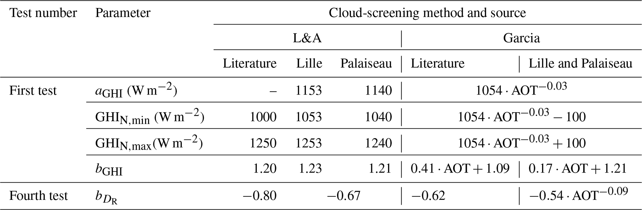
Table 1 compares the initial values of the coefficients from Long and Ackerman (2000) and García et al. (2014) with the ones found for our study conducted in Lille and Palaiseau over the period of 2010–2020. The parameters GHIN,min and GHIN,max correspond to the normalised global irradiance thresholds used in the first test to constrain GHIN. These thresholds are computed as W m−2. The application of the initial L&A method in Lille and Palaiseau produces equivalent scalable parameters, GHIN,min, GHIN,max, bGHI, and , for both sites.
García et al. (2014) modify the L&A method to make it applicable to the particular conditions of the Izana Observatory in the Canary Islands, a high-elevation arid site. They show that the daily mean coefficients aGHI,day and bGHI,day found for that site were somewhat correlated to the variations in AOT measured coincidentally at 500 nm. Note that as aerosol loadings are quite different between the Canary Islands and northern France, a parametrisation more representative of the specific conditions of Lille and Palaiseau was defined in this study. The variation in aGHI,day with respect to AOT in Lille and Palaiseau was found to be similar to the one used in García et al. (2014). However, the correlation coefficient is only 0.20, which is lower than the value reported by García et al. (2014). Additionally, the correlation coefficient for bGHI is only 0.30, which is significantly smaller than the value of García et al. (2014).
In the present study, the variability of the coefficient relative to AOT is also investigated using various parameterisations. The highest correlation coefficient of 0.31 is found when using a power law of AOT. Since this correlation coefficient is close to the one found for bGHI, we modify the Garcia method slightly by including the change in with respect to AOT (Table 1).
4.3 Impact of the cloud-screening procedures
Table 2 shows averaged values of the observed solar resource parameters in 2018–2019, under both all-sky and clear-sky conditions and for both cloud-screening methods. In addition, Table 3 shows averaged values of the key atmospheric properties observed by AERONET, which are most relevant for radiative transfer simulations of the solar resource components under clear-sky conditions, and Fig. 1 shows the seasonal dependence of AOT and WVC. Note that for Table 3, we use AERONET Level 2.0 data, which are automatically cloud screened in the only solar direction (i.e. clear sun). When coincident photometric and irradiance measurements are available, we are able to select AERONET measurements coincident with cloud-free irradiance data points identified by either two irradiance cloud-screening methods (clear sun and sky). In what follows, SZA is constrained below 80°. Winter is composed of December–February, spring March–May, summer June–August, and autumn September–November.
Table 2Averaged solar resource components (GHIobs, DNIobs, DifHIobs) observed in Lille and Palaiseau in 2018–2019 in all-sky and clear-sky conditions at 1 min time resolution (SZA < 80°). The all-sky data set corresponds to all data points, while the clear-sky data set is composed of the only minutes identified as cloud-free by either the algorithm of Long and Ackerman (2000) (L&A) or the method of García et al. (2014) (Garcia). The second part of the table gives the number of all-sky minutes and the proportion (%) of clear-sky minutes in 2018–2019 for each season.
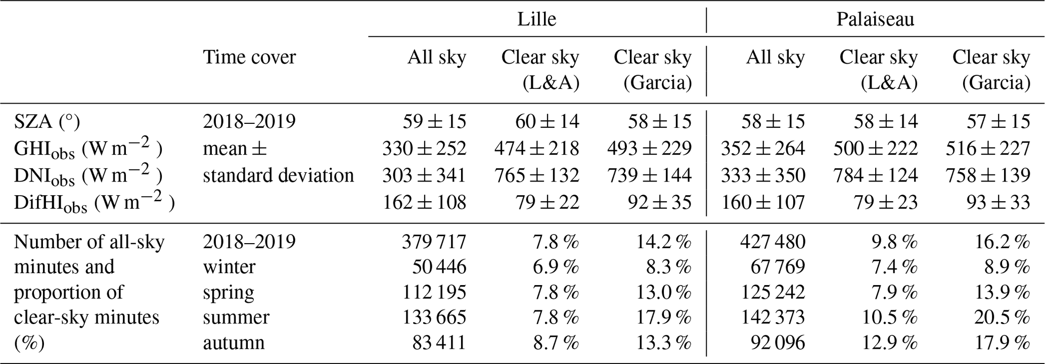
Table 3Average and standard deviation of instantaneous atmospheric properties measured in Lille and Palaiseau by AERONET in 2018–2019: AOT at 550 nm, the Ångström exponent α, and the water vapour column content (WVC). In clear-sun conditions, the number of observations represents the total number of Level 2.0 AERONET measurements, while in clear-sky conditions it corresponds to the number of minutes identified as cloud-free by either the algorithm of Long and Ackerman (2000) (L&A) or the method of García et al. (2014) (Garcia), coincident to the Level 2.0 AERONET data.

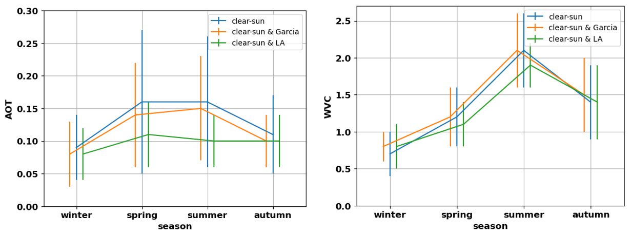
Figure 1Seasonal dependence of AOT and WVC (cm) in Lille in 2018–2019, according to Level 2.0 AERONET (blue), and for two cloud-screening methods (red for Garcia, green for LA). The vertical bars show the standard deviation for each season.
Overall, 14 % to 16 % of observed situations are identified as clear sky by the Garcia algorithm in 2018–2019 in Lille and Palaiseau, while clear skies only represent 8 % to 10 % of observations according to the stricter L&A cloud-screening method (Table 2). The proportion of clear-sky moments in summer is more than twice larger than in winter according to Garcia and larger by ∼ 35 % compared to spring and autumn. L&A also identifies less clear-sky moments in winter but unexpectedly does not show more clear-sky moments in summer than in spring and autumn. As written hereafter, the results show that L&A has a tendency to screen out moments characterised by large AOT values which occur more frequently in spring and summer (Table 3). Our analysis also shows that in 2018–2019, the accumulated amount of incident solar radiation (in W h m−2) under clear-sky conditions (Garcia method) represents 21.2 % and 23.7 % of the total accumulated GHI in Lille and Palaiseau, respectively.
The mean solar resource components are quite similar in Lille and Palaiseau, with almost equal DifHIobs values in both all-sky and clear-sky conditions (Table 2), indicating a comparable impact of the cloud cover. Nonetheless, DNIobs is larger in Palaiseau than in Lille, with a difference of about 30 W m−2 in all-sky conditions and approximately 20 W m−2 in clear-sky conditions. Part of these differences could be attributed to the smaller mean SZA in Palaiseau, which is located at a lower latitude than Lille. As a consequence, both all-sky and clear-sky GHIobs values are around 25 W m−2 larger in Palaiseau than in Lille.
As expected, the cloud-screening methods show a strong impact in GHIobs, DNIobs, and DifHIobs, although results vary between the two cloud-screening methods. The influence of the cloud-screening method is more important in DNIobs and DifHIobs than in GHIobs. For example, in Lille, DifHIobs is multiplied by a factor of 0.5–0.6 under clear-sky conditions, DNIobs by a factor of 2.3–2.5, and GHIobs by a factor of ∼ 1.45. Both cloud-screening methods have a comparable impact in DNIobs at both locations, which increases by 420–460 W m−2 from all-sky to clear-sky conditions. Conversely, DifHIobs in clear-sky conditions in Lille decreases by 83 W m−2 with L&A compared to all-sky conditions and by 70 W m−2 with Garcia. In this case, differences in DifHIobs between all-sky and clear-sky conditions are lower for the Garcia cloud-screening method, due to either aerosols or unfiltered clouds. The standard deviation in DifHIobs also strongly decreases from 67 % (compared to the average) in all-sky conditions in Lille to 38 % in clear-sky conditions with the Garcia method and to 28 % with the L&A method, and in DNIobs it strongly decreases from 113 % in all-sky conditions to 17 %–19 % in clear-sky conditions. L&A cloud-screening increases GHIobs by ∼ 145 W m−2, while Garcia cloud-screening increases GHIobs by ∼ 160 W m−2 in both Lille and Palaiseau. Compared to the L&A method, the Garcia method increases GHIobs by 16–19 W m−2.
The Level 2.0 AERONET clear-sun data set shows that the aerosol properties and WVC are highly variable in Lille and Palaiseau. The standard deviation is 71 % in AOT at 550 nm in Lille, 31 % in the Ångström exponent α, and 47 % in the WVC (Table 3). A significant part of this variability can be explained by seasonal changes, as mean AOT increases by a factor of 1.8 from winter to spring, and mean WVC increases by a factor of 3 from winter to summer (Fig. 1). The high variability of AOT and WVC is also related to intra-seasonal changes. This is particularly noticeable for AOT, with the standard deviation in spring remaining close to the standard deviation over a year. The 90th percentile of AOT in Lille is 0.32 in 2018–2019. AOT can be even larger than 0.80 as for example on both 6 June 2018 and 31 March 2019 or during the documented severe aerosol pollution episode of March 2014, with measured AOT reaching values of up to 0.90 in Lille and Palaiseau (Dupont et al., 2016; Favez et al., 2021).
The Garcia method keeps the seasonal influence of AOT while slightly reducing mean values and the standard deviation, mostly in spring–summer (Fig. 1), indicating that some large AOT events may be rejected by the cloud screening. However, the L&A method does not keep the seasonal influence of AOT, with an increase by only 0.02 from winter to spring and AOT remaining constant from summer to autumn. Moreover, the standard deviation is divided by more than 2 in spring–summer. Most large AOT events must be rejected by the L&A method. The seasonal dependence of α is not shown as it is not significant.
The annual averages in Lille and Palaiseau are close to the European average according to Gueymard and Yang (2020), based on AERONET, and also close to the average of the Cfb climate zone, embedding both sites (Gueymard and Yang, 2020). The differences between Lille and Palaiseau are small (Table 3), consistently with Ningombam et al. (2019), for the 1995–2018 time period. The averaged Level 1.5 AERONET aerosol single scattering albedo in Lille in 2018 is 0.97 ± 0.03 at 440 nm, 0.96 ± 0.04 at 675 nm, and 0.95 ± 0.04 at 870 nm (not shown in Table 3), depicting little absorption.
Our results also suggest that the clear-sky conditions identified by the Garcia cloud-screening method are more representative of the AOT variability observed in both Lille and Palaiseau than those detected with the L&A method:
-
The number of clear-sky minutes is larger in the Garcia data set than in the L&A data set (Table 3).
-
The annual means and standard deviations of AOT observed for clear skies identified by the Garcia cloud-screening method are closer to the clear-sun values than those obtained by the L&A method, especially in spring–summer when L&A significantly underestimates the clear-sun means (Fig. 1).
-
The relative increase in mean AOT from winter to spring for clear skies identified by the Garcia method is close to the increase observed under clear-sun conditions, while variability of AOT is less intense for the situations detected by the L&A method (Fig. 1).
This section presents the comparison scores between SolaRes computations of solar resource standard components (GHI, DNI, and DifHI) and ground-based measurements made in Lille and Palaiseau in 2018–2019. Furthermore, SolaRes computations are also compared to ground-based measurements of GTI in Lille in 2019.
Our analysis relies on two main statistical parameters: comparison of the relative mean bias difference (MBD) and the relative root mean square difference (RMSD), which are usual indicators of dispersion, as stated by Gueymard (2014), and have been used by many authors (e.g. Ruiz-Arias et al., 2013; Sun et al., 2019). MBD and RMSD values are computed as follows:
where obs stands for the observed quantity and comp for the SolaRes computation of any solar resource component: GHI, DNI, DifHI, and DifTI. The sum is made over the pair number N, obsmean stands for the averaged observed quantity, and the factor of 100 provides MBD and RMSD in percent. The best agreement between measurements and simulations is reached for the lowest values of MBD and RMSD.
Table 4Comparison scores (MBD and RMSD, Eq. 16) between GHIRT and GHIobs in both Lille and Palaiseau for the two cloud-screening procedures (Garcia and L&A as described in Sect. 4) over the whole 2018–2019 period (“all season”) and for each season. Note that CMP11 measurements of GHI in Lille are limited to the spring and summer of 2018. The number of comparison pairs (1 min resolution) and the corresponding averaged GHIobs are also given.
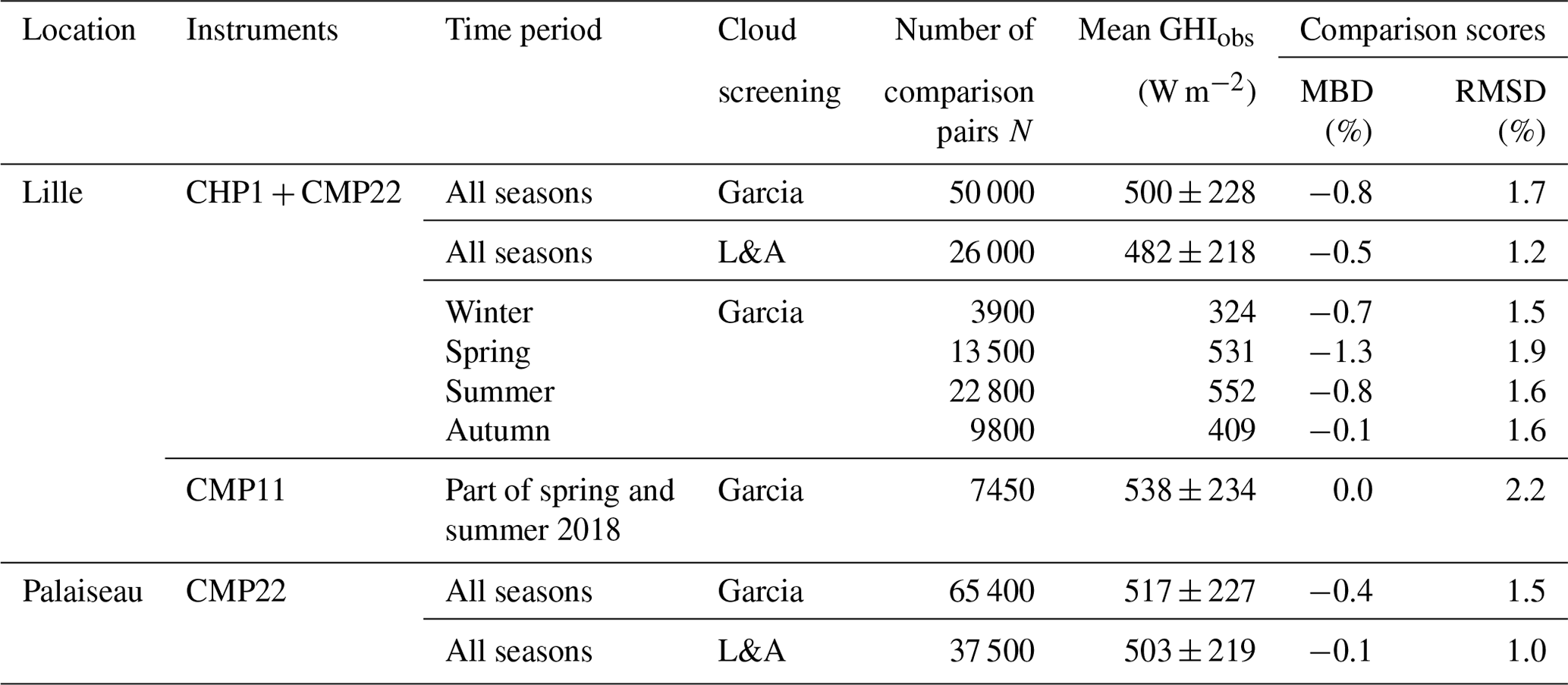
In this section, the continental clean and desert dust OPAC models are mixed to reproduce AERONET spectral AOT (Sect. 3.3). AERONET V3 provides not only the input spectral AOT, but also the WVC and the ozone column content. Daily averages of surface albedo delivered by the CAMS radiation service are used. The 3 min values are averaged at the 15 min time resolution. For the case of Lille in 2018–2019, 8500 radiative transfer computations of DifHI are performed at the 15 min time resolution and are then linearly interpolated at 1 min resolution. SolaRes provides solar resource components for 183 000 1 min time steps in clear-sun conditions. Only data within a temporal window of ±10 min around the AERONET record time are kept, and the SolaRes data set is then reduced to 125 000 time steps. A further screening is applied on SZA, keeping only values smaller than 80°, as was done by e.g. Ruiz-Arias et al. (2013). Comparison data pairs are generated by associating the coincident simulation and observation at 1 min time resolution. Eventually, the cloud-screening procedures on solar irradiance measurements (Sect. 4) are applied to limit comparisons to clear-sky conditions. Overall, in Lille in 2018–2019, 50 000 comparison data pairs are constituted with the Garcia cloud-screening procedure and 26 000 comparison data pairs with the L&A cloud-screening procedure (Table 4). Slightly more AERONET data are available for radiative transfer computations in Palaiseau over the same years, and more comparison pairs are eventually kept, namely ∼ 65 000 pairs with the Garcia cloud-screening method and 37 000 pairs with the L&A method.
As described in Sect. 2.1, GHIobs, DirHIobs, and DifHIobs are measured by four Kipp & Zonen instruments in both Lille and Palaiseau, and GTIobs is measured in Lille by a CMP11 pyranometer on a vertical plane. First, comparison scores in GHI are presented in Sect. 5.1 and then comparison scores in both DNI and DifHI, without (Sect. 5.2) and with (Sect. 5.3) the circumsolar contribution. Finally, Sect. 5.4 presents the comparison scores obtained for GTI computations on a vertical surface.
5.1 GHI in Lille and Palaiseau
Table 4 and Fig. 2 present the comparison scores in GHI. Overall, the correlation coefficient between GHIobs and GHIRT is 0.999 for the two sites (Fig. 2). For the “all-season” comparison involving CMP22, GHIobs is slightly underestimated by 0.4 % (Palaiseau) to 0.8 % (Lille) for clear skies identified by the Garcia cloud-screening method. The absolute underestimation is −3.8 ± 8.1 W m−2 in Lille, with 55 % of 1 min values included between −5 and 5 W m−2, which is within the uncertainty requirement for the measurements by BSRN (Ohmura et al., 1998). The RMSD in GHI is around 1.6 % in both Lille and Palaiseau with the Garcia cloud-screening method.

Figure 2Comparison between 1 min computations and observations in Lille in 2018–2019 (by CHP1 + CMP22) under clear-sky conditions, for GHI (a, d), DNI (b, e), and DifHI (c, f). Clear skies are identified by both the Garcia (a–c) and the L&A cloud-screening methods (d–f). Only comparison pairs with SZA < 80° and within 10 min of AERONET's record time of AOT are considered. MBD and RMSD are given according to Eq. (16), nb is the number of pairs, obsmean is the mean value of the observed solar resource component, and cc is the correlation coefficient of the linear interpolation (red line). The dashed grey line represents the x=y line.
The comparison of GHI involving CMP11 in Lille shows a better score in MBD and a worse score in RMSD than the CHP1 + CMP22 “all-season” comparison. The larger RMSD involving CMP11 seems partly correlated with the season. Indeed, the RMSD obtained with CHP1 + CMP22 in spring is 1.9 %, which is close to the RMSD of 2.2 % obtained with CMP11 in spring–summer and larger than the all-season RMSD of 1.7 %.
The smaller MBD obtained with the CMP11 pyranometer than with the CHP1 + CMP22 combination may be explained by the influence of the different spectral responses of CMP22 and CHP1 on one side and CMP11 on the other side. Indeed, according to SolaRes, the shorter spectral bandwidth of CMP11 reduces GHIRT by around 4.5 ± 2.5 W m−2 or 0.8 ± 0.3 %. This mean decrease in GHIRT, added to the mean negative bias obtained with the CHP1 + CMP22 combination, is close to the observed difference of 1.6 % between CMP11 and CHP1 + CMP22 GHIobs (Sect. 2.1). Consequently, MBD becomes negligible when comparing SolaRes estimates with CMP11 measurements.
Our results also show that the cloud-screening method has a significant impact on the comparison scores. For example, on 20 April 2018 between 12:00 and 14:00 UT in Lille, the largest disagreement in GHI occurs between the measurements and the SolaRes computations, with values of the difference reaching 60 W m−2 (Fig. 3). It is however limited to the Garcia method, as the L&A screening procedure gets rid of these points, consistently with its lower FPS by Gueymard et al. (2019). AERONET Level 2.0 provides values of AOT all day, meaning that no clouds are seen in the solar direction, and satisfying agreement in DNI indeed occurs between 12:00 and 14:00 UT (Fig. 3 middle). However significant disagreement occurs in DifHI, which is the cause of disagreement in GHI, suggesting the presence of clouds in the sky vault undetected by the Garcia cloud-screening method. Such a behaviour also happens twice later in the afternoon, with less intensity. During these three occurrences, the aerosol influence is well reproduced as we find agreement in DNI, and DifHI is systematically underestimated because of cloud presence in the sky vault (Fig. 3).

Figure 3GHI (a), DNIpyr (b), and DifHIpyr (c) observed (black line) in Lille on 20 April 2018 and also simulated by SolaRes (blue line). GHIobs is cloud screened by both Garcia (grey circles) and L&A methods (red dots).
Such a behaviour has consequences for the mean comparison scores over the full time period, as MBD and RMSD values decrease when considering only clear skies identified by the L&A cloud-screening procedure (Table 4 and Fig. 2). In particular, the L&A cloud-screening procedure decreases MBD in GHI by ∼ 0.3 % and RMSD by ∼ 0.5 %. MBD even reaches values as low as −0.1 % in Palaiseau with L&A, with 64 % of the MBD values lying within ±5 W m−2 of GHIobs. RMSD could be as low as 1.0 %, confirming the success of the radiative closure study involving pyranometers, AERONET AOT, and SolaRes.
5.2 DNI and DifHI without the circumsolar contribution
Both DNIobs and DifHIobs are separately measured in Lille and Palaiseau by the CHP1 pyrheliometer and the shaded CMP22 pyranometer, respectively. Tables 5 and 6 present the comparison scores for DNI and DifHI, respectively, as well as Fig. 2 (centre and right columns). In this section, the circumsolar contribution is not computed, DNIstrict is compared to DNIobs, and DifHIstrict is compared to DifHIobs.
Table 5As Table 4 but for DNIobs measured by the CHP1 pyrheliometer.
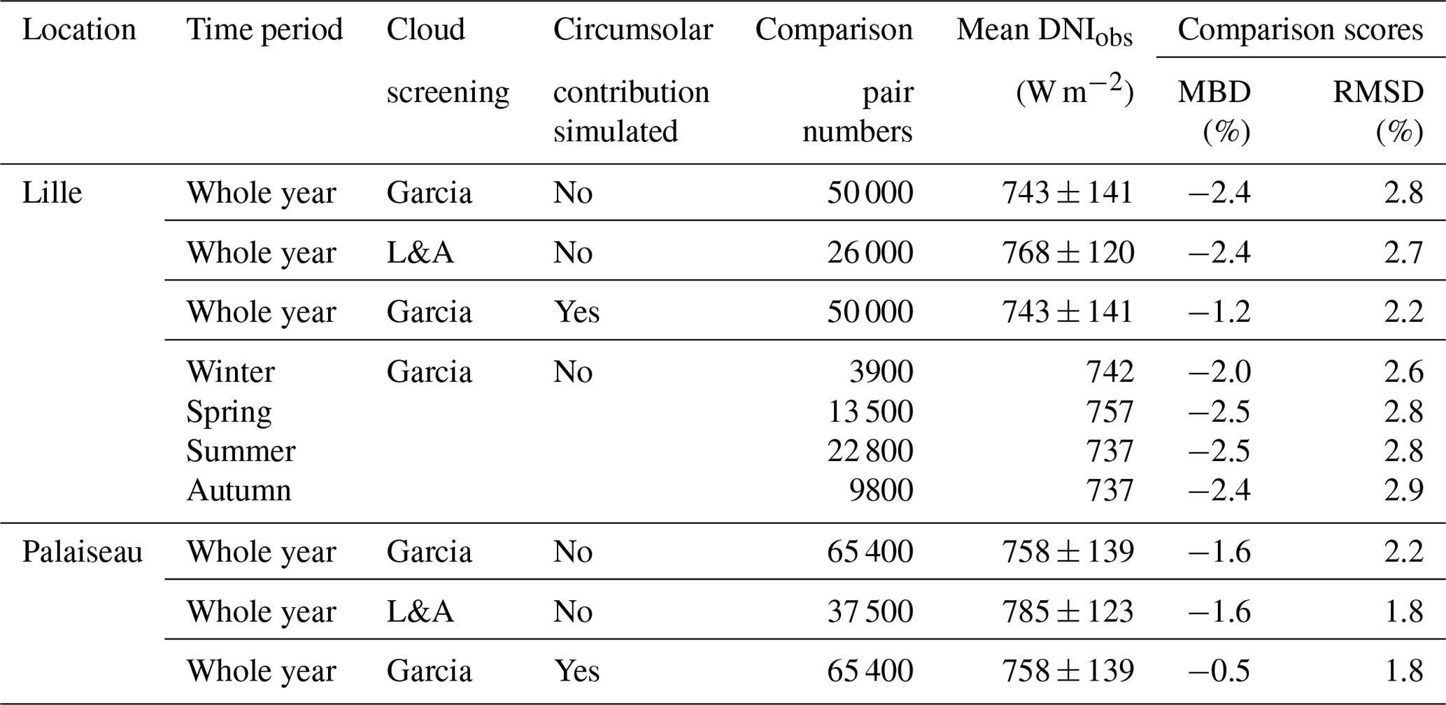
Table 6As Table 4 but for DifHIobs measured by the CMP22 pyranometer in 2018–2019.
Overall, DNIstrict is underestimated by −1.6 % in Palaiseau and −2.4 % in Lille (Table 5 and Fig. 2) with the Garcia cloud-screening method, and RMSD is 2.2 % in Palaiseau and 2.8 % in Lille. These results are highly satisfactory given the 5 % uncertainty in DNI claimed by Gueymard and Ruiz-Arias (2015) for an uncertainty of 0.02 in AOT (of AERONET measurements).
We can confidently guess negligible residual cloud influence in the solar direction as AERONET Level 2.0 screens out clouds in the solar direction, and it is moreover associated with the solar irradiance cloud-screening methods. The dependence of the comparison scores in DNI on the cloud-screening procedure is small, as the criteria on direct solar irradiance are similar between the two cloud-screening procedures. The different AOT ranges between the two cloud-screening methods do not affect the comparison scores.
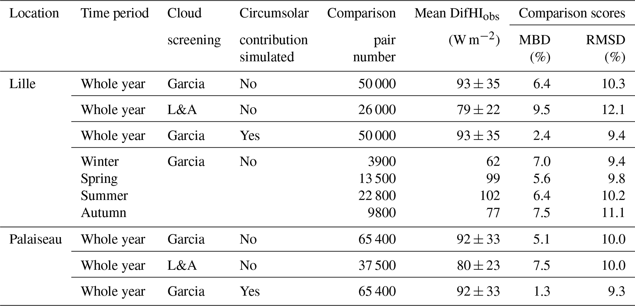
While DNIstrict is underestimated, DifHIstrict is overestimated, with MBD values of around 6 % in Lille and Palaiseau for clear skies identified with the Garcia cloud-screening method (Table 6 and Fig. 2). According to Eqs. (10) and (11), both DNIobs underestimation and DifHIobs overestimation are expected, as the circumsolar contribution is not considered here.
RMSD in DifHI is found to be of the order of 10 % at both stations, which is significantly larger than RMSD in both GHI and DNI. Better results in DNI than in DifHI are to be expected as AOT, which is the main input parameter of SolaRes, exclusively informs on aerosol extinction and mean size but neither on the proportion between scattering and absorption nor on surface reflection, which are both factors of DifHI but not of DNI. Moreover, uncertainty also arises from the interpolation procedure between 15 min estimates of DifHI with SMART-G. Eventually, the better agreement in GHI (Sect. 5.1) than in both DNI and DifHI shows that MBD in both DNI and DifHI mostly compensates for this.
It may be surprising that MBD in DifHI increases with the L&A cloud-screening procedure. This could be partly explained by the significant decrease in mean DifHI, as L&A screens out atmospheric conditions with the largest AOT and thus cases of higher diffuse irradiance. Similarly, MBD is significantly smaller in spring–summer than in autumn–winter, partly due to higher mean DifHI values.
Both mean GHIobs and mean DirHIobs are much larger in Palaiseau according to Gschwind et al. (2019) than with our cloud-screening procedures: GHIobs averaged over 2005–2007 is 600 W m−2, and mean DirHIobs is 492 W m−2 with a strict cloud-screening procedure keeping only ∼ 10 000 1 min data per year. Consequently, DifHIobs is 108 W m−2 for Gschwind et al. (2019), which is also larger than with our cloud-screening procedures. Indeed, annual mean GHIobs varies between 500 and 517 W m−2 in 2018 and 2019 in Palaiseau and DifHIobs between 79 and 93 W m−2, with (Tables 4 and 6) and without AERONET cloud screening (Table 2). According to Table 2, DirHIobs is ∼ 420 W m−2 when subtracting DifHIobs from GHIobs.
As shown in Sect. 4, when the cloud screening is stricter, atmospheric scattering is reduced, and DifHIobs may decrease, while on the contrary DNIobs may increase. As the Gschwind et al. (2019) data filtering increases both DifHIobs and DirHIobs, the cloud-screening strictness is not in play. Another important factor is SZA. We could then hypothesise that the Gschwind et al. (2019) data filtering procedure rejects large values of SZA; for example, the mean SZA would be smaller than in our data sets (Table 2), explaining the increase in both DirHIobs and DifHIobs and consequently in GHIobs.
5.3 DNI and DifHI with the circumsolar contribution
In this section, we consider DNIpyr and DifHIpyr, which are corrected by the circumsolar contribution to better represent the measurements, according to Eqs. (10) and (11). The circumsolar contribution to the direct normal radiation, ΔDifNIcirc, is found to be 8 ± 6 W m−2 on average (similar in both sites), with a median and a 90th percentile of 6 and 15 W m−2, respectively. ΔDifNIcirc then represents 1.2 ± 1.3 % of DNIstrict, with a median of 0.7 % and a 90th percentile of 2.4 %. Figure 4 shows ΔDifNIcirc as a function of both the Ångström exponent α and the slant aerosol optical thickness at 550 nm (SOT), which is defined as AOT divided by μ0 (Blanc et al., 2014). Most values of ΔDifNIcirc are smaller than 20 W m−2, consistently with simulations by Blanc et al. (2014). Values larger than 20 W m−2 mostly occur for small α and/or large SOT.
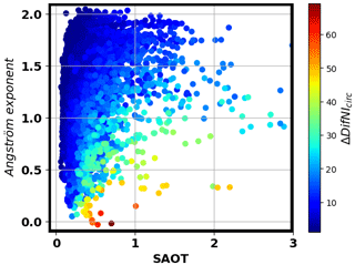
Figure 4The circumsolar contribution ΔDifNIcirc (W m−2) as a function of both the Ångström exponent α and the slant-path optical thickness at 550 nm (SOT) in Lille in 2018.
Overall, adding ΔDifNIcirc to DNIstrict improves the comparison scores, with a decrease in both MBD and RMSD in DNI, by more than 1 % and ∼ 0.5 %, respectively (Table 5). The mean circumsolar contribution to diffuse horizontal irradiance, ΔDifHIcirc, is 4 ± 2 W m−2, and the comparison scores with DifHIpyr also significantly improve, with MBD decreasing by more than 4 % and RMSD slightly decreasing by less than 1 % (Table 6).
5.4 Diffuse irradiance on a vertical plane
5.4.1 Two regimes
GTIobs is measured in Lille from 18 January to 31 December 2019 by the CMP11 pyranometer, with the instrument being tilted vertically at 90° and facing southward (i.e. azimuth angle of 180°). The signal in summer shows two distinct regimes, as for example on 27 June 2019 (Fig. 5):
-
For most of the day around noon, the sun, positioned in the southern-half sky, faces the instrument and is thus included in the instrument field of view. Both diffuse and direct radiation contribute to the observation.
-
At both the beginning and the end of the day, the sun could be positioned behind the instrument in the northern-half sky, the instrument sensor then being in the shadows. Only diffuse radiation is observed, which is less dependent on SZA than direct radiation, generating wings at the end of the day that are flatter than around noon.
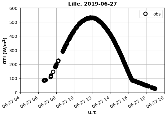
Figure 5Global tilted irradiance (GTIobs) observed by the CMP11 pyranometer on a vertical plane facing south, on 27 June 2019 in Lille. The sun is southwards between 07:14 and 16:27 UT.
Comparisons are made in both regimes independently (Table 7).
Table 7As Table 4 but for GTI on the vertical plane facing south in Lille in 2019 for clear skies identified with the Garcia cloud-screening procedure. The time period is defined by the season and by the range of SAA. Computations are also made for different values of the surface albedo.

5.4.2 Diffuse contribution at both the beginning and the end of the day in summer
Comparison of GTI between observations and SolaRes simulations is made by selecting SAA larger than 270° (end of the day in summer). Around a thousand comparison pairs are generated. Overall, observation tends to be overestimated by 6 %, and the RMSD is 8.5 % (first line in Table 7). Similarly, by selecting SAA smaller than 90° (beginning of the day), the overestimation is 8.7 %, and the RMSD is 12.1 %. These results are similar to the comparison scores in DifHI (Table 6).
5.4.3 The influence of changing surface albedo on GTI
Comparison between the observation and simulation for the sun facing the instrument (90° < SAA < 270°) shows that GTIobs can be accurately reproduced but with an RMSD of 5 % (third line in Table 7). The overall larger RMSD in GTI than in GHI (Table 4) is partly caused by the variability in the effective surface albedo.
By distinguishing winter and summer seasons, MBD changes from +3.7 % in summer to −6.5 % in winter (fourth and fifth lines in Table 7). Although changes in the surface albedo derived from satellite observations appear to be small, computations for 26 February 2019 show that observations can be reproduced with an effective surface albedo of 0.35 (Fig. 6). The underestimation in winter then decreases from 6.5 % to 0.2 %, and RMSD decreases down to 1.4 % (sixth line in Table 7), which is similar to results in GHI (Table 4). Heterogeneities in the albedo of buildings' walls at local scale and subsequent 3D effects could be responsible for such differences between a satellite surface albedo and an effective surface albedo for a vertical instrument. The differences between winter and summer seasons could be caused by fallen leaves of surrounding trees, in relation to the sun position in the sky. Consistently with our results, Mubarak et al. (2017) also show that the surface albedo has a significant effect on estimating GTI on a vertical plane (but with a transposition model).
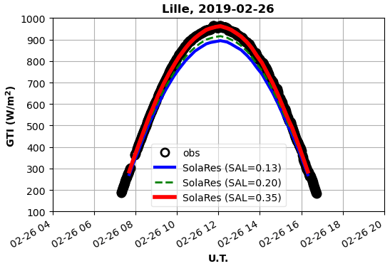
Figure 6The same as Fig. 5 but for 26 February 2019 and with SolaRes estimates for different values of the surface albedo (SAL). According to MODIS, the daily average of the surface albedo is 0.13.
This section shows the sensitivity of the computed solar resource parameters to the parameterisation of the aerosol properties and also to the aerosol data source.
Atmospheric optical properties are necessary input data of a radiative transfer code. In clear-sky conditions, aerosols are the main source of variability of the atmospheric optical properties. Necessary aerosol optical properties are the optical thickness, the phase function, and the single scattering albedo at any wavelengths. Measurements are exploited to reproduce the temporal variability in aerosol optical properties. However, measurements can rarely provide all necessary optical properties, such as the full phase function and the single scattering albedo. It is therefore necessary to employ various strategies to get the necessary parameters from observation data sets. For example, the measured data set can be inverted to provide a fully described microphysical aerosol model, assuming some hypotheses, which is then usable in radiative transfer computations. AERONET provides such inverted aerosol models at a resolution of around 1 h. For the validation, we prefer relying on the highest sampling rate by AERONET at 3 min, which detects and best describes most aerosol events, with spectral AOT. AOT measured at the two wavelengths of 440 and 870 nm is used in SolaRes to constrain the mean aerosol burden and also as an indicator of the mean aerosol size. Two aerosol OPAC models are mixed in such proportions that they reproduce the observed AOT (Eq. 12) and all necessary aerosol optical properties. First, performances of SolaRes computations are compared for various combinations of the OPAC aerosol models (Sect. 6.1). The influence of the input data source is also evaluated by testing the CAMS-NRT regular-grid global data set as input data of SolaRes (Sect. 6.3).
6.1 Impact of the aerosol parameterisation: the aerosol model combination
While validation in Sect. 5 is performed with a mixture of continental clean and desert dust aerosol OPAC models, the aerosol models are changed here to show the sensitivity of the solar resource parameters to the aerosol parameterisation. To best reproduce the observed AOT spectral variability, an aerosol model mainly composed of relatively small aerosols (producing large α) is mixed with an aerosol model composed of larger aerosols (producing small α). The large-α aerosol models are named by OPAC as continental clean, continental polluted, and urban, and the small-α aerosol models are named desert dust, maritime clean, and maritime polluted. Table 8 shows the impact of several aerosol model combinations on the comparison scores between the observation and simulations, which include the circumsolar contribution. In this subsection, only clear-sky moments identified by the Garcia cloud-screening method are selected in Lille in 2018.
Table 8Sensitivity of the solar resource components to the OPAC aerosol models in terms of MBD and RMSD in GHI, DNIpyr, and DifHIpyr. As large-α models, cc stands for continental clean, cp for continental polluted, and ur for urban. As small-α models, dd stands for desert dust, mc for maritime clean, and mp for maritime polluted. Comparisons are made with observations made in 2018 in Lille for clear skies identified by the Garcia cloud-screening method.
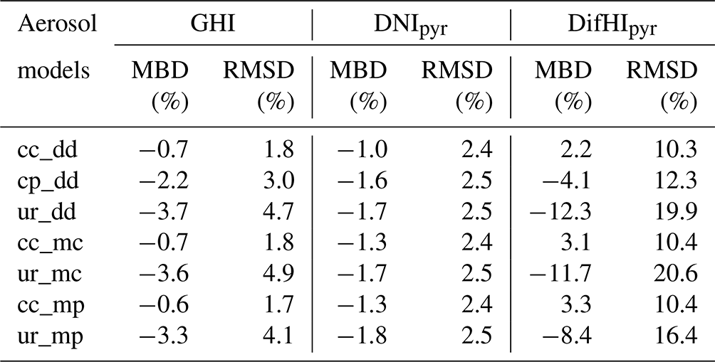
DNIpyr is the least sensitive parameter to the various combinations of aerosol models, with MBD changing between −1.3 % and −1.7 % and RMSD remaining around 2.5 % (Table 8). This low sensitivity is expected as only the circumsolar contribution in DNIpyr depends on the angular scattering (phase function) and on the absorption of solar radiation (aerosol single scattering albedo). DifHIpyr does however depend on both the phase function and the single scattering albedo and is thus much more dependent on the aerosol models than DNIpyr. The mean absorption coefficient increases from continental clean to continental polluted and the urban model, leading to a decrease in DifHIpyr and a significant decrease in MBD from ∼ +3 % (continental clean) to ∼ −12 % (urban). In contrast, the small-α model shows less influence than the large-α model (Table 8).
As a result, the aerosol model mixture significantly affects GHI simulations, mainly because of the sensitivity of DifHIpyr to the large-α aerosol model. The efficient compensation between DNIpyr underestimation and DifHIpyr overestimation mostly occurs with the continental clean (cc) model, which provides the best scores in GHI, with an MBD of −0.7 % and an RMSD of 1.8 % in 2018 in Lille. This is consistent with the large value of averaged SSA in Lille in 2018, as inverted from AERONET measurements.
The choice of the small-α aerosol model has little influence on GHI. It is pertinent to choose desert dust as it can be transported to Europe from northern Africa (Papayannis et al., 2008).
6.2 Impact of the aerosol parameterisation: the AERONET-inverted aerosol optical properties as data source instead of spectral AOT
In this subsection, the AERONET-inverted aerosol model is exploited by SolaRes, replacing the spectral AOT parameterisation.
The time resolution of the AERONET-inverted aerosol model is around 1 h, and 420 time records are available in 2018 in Lille instead of the ∼ 13 000 Level 2.0 AOT time records. As with the AOT reparametrisation, computations are interpolated at 1 min, but the ±10 min condition is not applied here in order to get as many 1 min data pairs as possible.
Table 9The same as Table 4 but for GHI, DNIpyr, and DifHIpyr in Lille in 2018. The AERONET-inverted aerosol model composes the input data set of SolaRes.
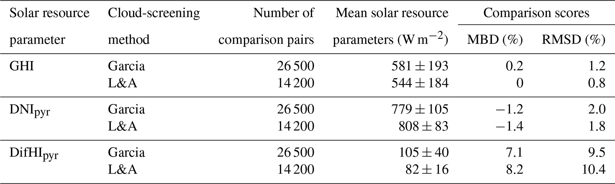
Table 9 shows the comparison scores between observations and simulations for GHI, DNIpyr, and DifHIpyr. The RMSD in GHI decreases from 1.7 % to 1.2 % with Garcia and from 1.2 % to 0.8 % with L&A (compared to scores in Table 4), while MBD becomes negligible for both cloud-screening methods. Ruiz-Arias et al. (2013) also compare the observation and computations, exploiting Level 1.5 AERONET-inverted products with a radiative transfer code, but for smaller mean AOT. In GHI, our performances are similar to Ruiz-Arias et al. (2013) comparison scores, with an RMSD of ∼ 1 % and MBD of 0 %. Such a high performance is also attained with the AERONET spectral AOT parameterisation in Palaiseau and the L&A cloud-screening method (Table 4). We demonstrate the high performance of SolaRes in GHI with the 1 min resolution over at least a year, making SolaRes consistent with scientific and industrial applications. Ruiz-Arias et al. (2013) also show significant spatial variability of the comparison scores, with MBD changing from 0 % to −1 % depending on the site. Similarly, Sect. 5.1 also presents 0.4 % difference in MBD between Lille and Palaiseau.
The performances in DNI do not significantly improve with the AERONET-inverted models, showing that the simpler approach based on spectral AOT is appropriate to get high precision in DNIpyr (Table 5). Ruiz-Arias et al. (2013) present an MBD of 0 % but which would be expected to be negative as no circumsolar contribution is computed. The RMSD in DNIpyr with SolaRes is twice as large as that presented by Ruiz-Arias et al. (2013), but it accounts for larger mean AOT in Lille and Palaiseau compared to their data sets.
The AERONET-inverted aerosol model slightly improves DifHIpyr simulations. Moreover, MBD remains positive, which is in agreement with the tendency of overestimation shown by Ruiz-Arias et al. (2013). In addition, Ruiz-Arias et al. (2013) also showed spatial variability of comparison scores, and our scores for DifHIpyr are similar to those presented for one of their sites but where the mean AOT is smaller than in Lille in 2018. As the inverted AERONET aerosol model is expected to be the best model, the remaining discrepancies could be linked to other sources, notably the surface reflection model in SolaRes. According to AERONET inversion products, the surface albedo in Lille at 440 and 675 nm is smaller than what is used in the present study. Reducing the surface albedo should indeed reduce DifHI and the MBD. However, studying the sensitivity to surface albedo is beyond the scope of this paper.
6.3 Impact of the input data source: reanalysis global data set
AERONET provides observations of columnar aerosol optical properties with the best precision and accuracy. However, the AERONET data sets are site-specific and present limited spatial coverage of the Earth, despite an increasing number of stations. To provide solar resource parameters anywhere on the globe, it is necessary to use a global data set defined on a regular grid and on a constant time step, such as that provided by global transport and chemistry models used in CAMS and Modern-Era Retrospective Analysis for Research and Applications, version 2 (MERRA-2) (Gelaro et al., 2017), programmes. Compared to AERONET, such data sets exhibit large uncertainties (Gueymard and Yang, 2020); it is consequently important to evaluate their influence on the computed solar resource components (GHI, DNI, DifHI).
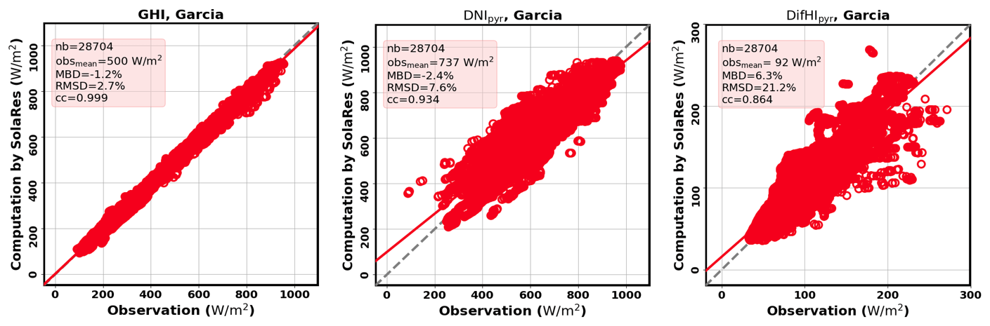
Figure 7The same as Fig. 2 for solar resource parameter comparisons in Lille but for CAMS-NRT as input data source instead of AERONET, using the Garcia cloud-screening procedure applied in 2018 (no AERONET cloud screening). GHI, DNIpyr, and DifHIpyr are showed.
Comparison between observations and simulations is performed in Lille in 2018 with CAMS-NRT (Sect. 2.4) instead of AERONET. The cloud screening is now based uniquely on solar irradiance measurements and not on the AERONET Level 2.0 clear-sun method. As expected, SolaRes simulations present higher RMSD values for all solar resource components with CAMS-NRT than with AERONET. RMSD in GHI increases by 0.6 % to 0.8 % and reaches 2.7 % with the Garcia cloud screening (Fig. 7) and 1.8 % with the L&A cloud screening (not shown). The cloud-screening influence is found to be 0.9 % with the CAMS-NRT data set, while it is 0.5 % with the AERONET spectral AOT parameterisation (Sect. 5.1).
The impact is larger in DNIpyr and DifHIpyr, with the RMSD in DNIpyr increasing by ∼ 5 % to reach 7.6 % and RMSD in DifHIpyr increasing by more than 10 %. This is consistent with Ruiz-Arias et al. (2013), who stated that “the impact of aerosols in direct surface irradiance is about three to four times larger than it is in global surface irradiance”, quoting Gueymard (2012). A test was done by adding the Level 2.0 AERONET clear-sun method, reducing the RMSD in DNIpyr by only 0.3 %. Witthuhn et al. (2021) show that the increased RMSD for both GHI and DNI is caused by the dispersion of CAMS AOT compared to AERONET. Their results over Germany in 2015 are similar to ours, with RMSD values of 3.2 %, 8.6 %, and 15.2 % in GHI, DNI, and DifHI, respectively, using CAMS reanalysis and a different cloud-screening procedure. Note however that their results show an overestimation of the simulated DNI compared to observations, in contrast with SolaRes results. Moreover, Salamalikis et al. (2021) evaluate a 7.7 % RMSD in DNI caused by CAMS reanalysis AOT compared to AERONET AOT in western Europe, while we have a 5 % increase. The RMSD between observations and SolaRes GHI remains smaller than the best score of 3.0 % provided by Sun et al. (2019) for many sites. The main differences from our comparison study is that Sun et al. (2019) use the MERRA-2 data set instead of CAMS-NRT. Additionally, their scores are obtained for a much larger observation data set, which is more representative of the global variability of aerosol properties than the measurements in Lille and Palaiseau.
The SolaRes tool, based on the radiative transfer code SMART-G, aims to estimate solar resource components with precision and accuracy anywhere on the globe, for a variety of meteorological and ground surface conditions and for any solar plant technology. SolaRes is designed for a large number of scientific to industrial applications by producing time series at 1 min time resolution and covering all situations for more than a year, with acceptable computational speed. Input parameters are atmospheric optical properties as the spectral aerosol and cloud optical thickness, which are usually available in many data sets.
As a first step in the comprehensive validation process, this paper evaluates SolaRes retrievals in clear-sky conditions by comparison to ground-based measurements of surface solar irradiance from two sites north of France. This approach aims to assess the main roles of aerosols, whose influences dominate in the absence of clouds, when GHI and DNI are maximum. Aerosol and water vapour parameters can be measured coincidently and precisely by the ground-based instrumentation of AERONET, and the validation in clear-sky conditions is then a radiative closure study.
We perform comparisons between SolaRes estimates and ground-based measurements of the solar resource components (GHI, DNI, DifHI) performed in 2018–2019 in Lille (ATOLL) and Palaiseau (BSRN site) at 1 min time resolution. GHIobs is slightly underestimated by SolaRes (0.1 %), with a mean RMSD of around 1.0 % in Palaiseau when a strict cloud-screening method based on Long and Ackerman (2000) (L&A) is applied, which also filters out conditions with the largest AOT, such as those occurring in spring and summer. Another cloud-screening method based on García et al. (2014) (hereafter Garcia) is used, which is more representative of the aerosol variability conditions. With this cloud-screening method, underestimation slightly worsens to 0.4 % in Palaiseau and 0.8 % in Lille, partly because of residual clouds increasing observed DifHI, and RMSD increases to ∼ 1.6 %. The impact of the cloud-screening method in GHI is 0.5 % of RMSD and 0.3 % of mean bias difference (MBD). Thereafter, unless stated otherwise, results are given with the Garcia cloud-screening method, which is more representative of the aerosol conditions over northern France.
SolaRes is able to consider various spectral bandwidths, and results are found to be similar with another instrument operating in a slightly restricted spectrum. SolaRes also performs well in reproducing the angular features of the solar radiation field. Indeed, the comparison scores in both DNI and DifHI improve by considering the circumsolar contribution. Underestimation of DNIobs by SolaRes decreases by 1 % to reach an MBD of −1.0 % by considering the circumsolar contribution, and the RMSD also decreases slightly to reach ∼ 2 %. Overestimation of DifHI by SolaRes decreases by ∼ 4 % to reach an MBD of 3 % in Lille and 2 % in Palaiseau, with an RMSD of 10 %. It is interesting to note that DNI underestimation and DifHI overestimation mostly compensate for each other to provide mean overall agreement in GHI.
The advantages of using SolaRes for solar resource estimates with tilted panels are twofold: (1) DNI and DifHI are correctly computed, even considering the circumsolar contribution for comparison purposes with observations, and (2) diffuse irradiance on a titled plane (DifTI) can be computed by radiative transfer computations, thus avoiding uncertainties associated with transposition models (i.e. Mubarak et al., 2017). Comparisons with measurements performed in Lille on a vertical plane facing south show satisfying agreement for DifTI with an RMSD of 8 %. It is suggested that there is a strong influence of reflection from not only the ground surface but also the surrounding buildings, and this influence changes with the season. Indeed, the global irradiance on a tilted plane (GTI) measured exclusively in winter could be reproduced with the same scores as GHI but with an increased surface albedo from 0.13 to 0.35.
Input spectral AOT allows us to constrain both mean aerosol extinction and size but neither the aerosol absorption nor the angular behaviour of aerosol scattering. A hypothesis is thus necessary to complement the aerosol model in order to perform radiative transfer computations, and two aerosol models of the OPAC database are combined to reproduce input spectral AOT. A sensitivity study of the solar resource components is conducted by changing the two aerosol models. It shows that the input spectral AOT efficiently constrains DNI regardless of the aerosol models, while DifHI is highly sensitive to the aerosol models. Indeed, SolaRes DifHI significantly decreases with increasing aerosol absorption of the aerosol model, and MBD in DifHI becomes negative with urban aerosols instead of continental clean aerosols. Consequently, GHI underestimation could worsen to 2 %, and RMSD in GHI could increase to 4 %. We found that the best combination in Lille and Palaiseau consists of a continental clean aerosol model mixed with a desert dust model. Further tests with the aerosol models inverted by AERONET show significant improvement in GHI by decreasing MBD to 0.2 % and by decreasing RMSD by 0.5 %. RMSD in GHI could be even smaller than 1 % in Lille with the L&A cloud screening. In conclusion, SolaRes can reproduce GHI at 1 min resolution, with negligible bias and an RMSD smaller than 1 %, with appropriate input data on aerosols, which are spectral AOT in Palaiseau or an AERONET-inverted model in Lille. With the Garcia cloud-screening method being more representative of aerosol conditions, MBD remains smaller than 0.5 % and RMSD smaller than 1.5 %.
Comparisons are also done in the SolaRes global mode by using input AOT delivered by CAMS-NRT instead of AERONET. The RMSD in GHI increases by 0.6 %–1.0 % and becomes 1.8 % with the L&A cloud-screening method and 2.7 % with Garcia. The RMSD in DNI increases by ∼ 5 % and by more than 10 % in DifHI. Scores also depend on the site, as RMSD in GHI is smaller by ∼ 0.2 % in Palaiseau compared to Lille and MBD by 0.4 %.
Perspectives consist of validating SolaRes in more diverse conditions, such as an arid environment strongly affected by desert dust, as has already been done for DNI with the ASoRA method (Elias et al., 2021). To complete the validation in all-sky conditions, the simulation of the cloud's influence by SolaRes in the global mode will be evaluated against ground-based measurements. More studies are also necessary for computations on tilted planes, investigating the influence of the environment on the reflection of the solar radiation. SolaRes may be improved by considering the spectral dependence of surface albedo and even the bidirectional reflectance distribution function, especially when dealing with solar resource assessment on tilted planes. Solar resource can also be evaluated in a complex physical environment embedded in a realistic changing atmosphere, even considering 3D interactions between solar radiation and the environment. Moulana et al. (2019) present preliminary work on the increased precision on solar resource assessment in a tower-concentrated thermal solar plant using SMART-G, and Moulana et al. (2024) present the technology to adapt SMART-G to consider reflection with 3D objects.
For now SolaRes is not made available because it still demands code development. SMARTG is owned by HYGEOS and is available for research activities on the following repository: https://github.com/hygeos/smartg (Ramon et al., 2024, 2019).
AERONET data are available at https://aeronet.gsfc.nasa.gov/new_web/draw_map_display_aod_v3.html (NASA, 2024). CAMS radiation data are available at https://ads.atmosphere.copernicus.eu/cdsapp/#!/dataset/cams-global-atmospheric-composition-forecasts?tab=form (ECMWF, 2024). The radiation data set from the Palaiseau BSRN site is accessible at https://bsrn.awi.de/ (last access: 3 July 2024) or https://dataportals.pangaea.de/bsrn/ (WRMC, 2024). The radiation data set from the ATOLL platform in Villeneuve-d'Ascq, north of France, has been published for the period 2010–2022 in the data repository https://doi.org/10.57932/ca9c74c0-83f4-43f1-86c8-7f3ce517b03c (Chesnoiu et al., 2024). This data set contains irradiance measurements, coincident aerosol, and gas column properties from AERONET, and the Garcia clear-sky flag is freely available from an EASY system data repository.
GC wrote Sect. 4 and developed the cloud-screening codes. TE and MM developed the SolaRes code, and TE made the SolaRes computations for the paper. TE wrote the other sections of the paper. NF is the principal investigator of the Lille instrument. NF and IC are the PhD supervisors of GC. All authors contributed to discussions about the work in progress and to writing the paper.
The contact author has declared that none of the authors has any competing interests.
Publisher’s note: Copernicus Publications remains neutral with regard to jurisdictional claims made in the text, published maps, institutional affiliations, or any other geographical representation in this paper. While Copernicus Publications makes every effort to include appropriate place names, the final responsibility lies with the authors.
The authors would like to thank people from LOA – Frédérique Auriol, Diane Catalfamo, and Isabelle Jankowiak – who contribute to the continuous monitoring of solar irradiance, which includes GHI, DNI, DifHI, and GTI from the ATOLL platform, and BSRN and the station PIs (Martial Haeffelin/Jordi Badosa) for the observation data set of Palaiseau, which includes GHI, DNI, and DifHI. AERONET is also acknowledged for the data set of AOT, WVC, and inverted aerosol model products, as well as Philippe Goloub, the PI of the Lille and Palaiseau stations. CAMS is also acknowledged for providing the AOT data.
Work for this study by Gabriel Chesnoiu was done during his PhD thesis financed by the ADEME and Région Hauts-de-France.
This paper was edited by Alexander Kokhanovsky and reviewed by three anonymous referees.
Anderson, G. P., Clough, S. A., Kneizys, F. X., Chetwynd, J. H., and Shettle, E. P.: AFGL (Air Force Geophysical Laboratory) atmospheric constituent profiles (0.120 km), Environmental research papers, United States, https://apps.dtic.mil/sti/citations/ADA175173 (last access: 28 June 2024), 1986.
Beck, H. E., Zimmermann, N. E., McVicar, T. R., Vergopolan, N., Berg, A., and Wood, E. F.: Present and future Köppen-Geiger climate classification maps at 1-km resolution, Sci. Data, 5, 180214, https://doi.org/10.1038/sdata.2018.214, 2018.
Benedetti, A., Morcrette, J.-J., Boucher, O., Dethof, A., Engelen, R., Fisher, M., Flentje, H., Huneeus, N., Jones, L., Kaiser, J., Kinne, S., Mangold, A., Razinger, M., Simmons, A. J., and Suttie, M.: Aerosol analysis and forecast in the European centre for medium-range weather forecasts integrated forecast system: 2. Data assimilation, J. Geophys. Res.-Atmos., 114, D13205, https://doi.org/10.1029/2008JD011235, 2009.
Blanc, P., Espinar, B., Geuder, N., Gueymard, C., Meyer, R., Pitz-Paal, R., Reinhardt, B., Renné, D., Sengupta, M., Wald, L., and Wilbert, S.: Direct normal irradiance related definitions and applications: The circumsolar issue, Sol. Energy, 110, 561–577, 2014.
Bodhaine, B. A., Wood, N. B., Dutton, E. G., and Slusser, J. R.: On Rayleigh Optical Depth Calculations, J. Atmos. Ocean. Tech., 16, 1854–1861, https://doi.org/10.1175/1520-0426(1999)016<1854:ORODC>2.0.CO;2, 1999.
Bogumil, K., Orphal, J., Voigt, S., Spietz, P., Fleischmann, O. C., Vogel, A., Hartmann, M., Kromminga, H., Bovensmann, H., and Burrows, J. P.: Measurements of Molecular Absorption Spectra with the SCIAMACHY Pre-Flight Model: Instrument Characterization and Reference Data for Atmospheric Remote-Sensing in the 230–2380 nm Region, J. Photochem. Photobio. A., 157, 167–184, 2003.
Chen, C., Dubovik, O., Schuster, G. L., Fuertes, D., Meijer, Y., Landgraf, J., Karol, Y., and Li, Z.: Characterization of temporal and spatial variability of aerosols from ground-based climatology: towards evaluation of satellite mission requirements, J. Quant. Spectrosc. Ra., 268, 107627, https://doi.org/10.1016/j.jqsrt.2021.107627, 2021.
Chesnoiu, G., Ferlay, N., and Chiapello, I.: Ground measurements of surface solar irradiance, aerosol optical properties and sky conditions estimates in Lille (North of France) over the period 2010–2022, Earth System Data Repository [data set], https://doi.org/10.57932/ca9c74c0-83f4-43f1-86c8-7f3ce517b03c, 2024.
Driemel, A., Augustine, J., Behrens, K., Colle, S., Cox, C., Cuevas-Agulló, E., Denn, F. M., Duprat, T., Fukuda, M., Grobe, H., Haeffelin, M., Hodges, G., Hyett, N., Ijima, O., Kallis, A., Knap, W., Kustov, V., Long, C. N., Longenecker, D., Lupi, A., Maturilli, M., Mimouni, M., Ntsangwane, L., Ogihara, H., Olano, X., Olefs, M., Omori, M., Passamani, L., Pereira, E. B., Schmithüsen, H., Schumacher, S., Sieger, R., Tamlyn, J., Vogt, R., Vuilleumier, L., Xia, X., Ohmura, A., and König-Langlo, G.: Baseline Surface Radiation Network (BSRN): structure and data description (1992–2017), Earth Syst. Sci. Data, 10, 1491–1501, https://doi.org/10.5194/essd-10-1491-2018, 2018.
Dubovik, O., Smirnov, A., Holben, B. N., King, M. D., Kaufman, Y. J., Eck, T. F., and Slutsker, I.: Accuracy assessments of aerosol optical properties retrieved from AERONET sun and sky-radiance measurements, J. Geophys. Res., 105, 9791–9806, 2000.
Dupont, J.-C., Haeffelin, M., Badosa, J., Elias, T., Favez, O., Petit, J. E., Meleux, F., Sciare, J., Crenn, V., and Bonne, J. L.: Role of the boundary layer dynamics effects on an extreme air pollution event in Paris, Atmos. Environ., 141, 571–579, https://doi.org/10.1016/j.atmosenv.2016.06.061, 2016.
ECMWF: CAMS global atmospheric composition forecasts, ECMWF [data set], https://ads.atmosphere.copernicus.eu/cdsapp/#!/dataset/cams-global-atmospheric-composition-forecasts?tab=form, last access: 3 July 2024.
Elias, T., Ramon, D., Brau, J.-F., and Moulana, M.: Sensitivity of the solar resource in solar tower plants to aerosols and water vapor, AIP Conf. Proc., 2126, 190006, https://doi.org/10.1063/1.5117703, 2019.
Elias, T., Ramon, D., Dubus, L., Am-Shallem, M., and Kroyzer, G.: DNI and slant path transmittance for the solar resource of tower thermal solar plants: The validation of the ASoRA method and impact in exploiting a global data set, Sol. Energy, 217, 78–92, https://doi.org/10.1016/j.solener.2020.12.064, 2021.
Emde, C., Buras, R., and Mayer, B.: Alis: An efficient method to compute high spectral resolution polarized solar radiances using the Monte Carlo approach, J. Quant. Spectrosc. Ra., 112, 1622–1631, 2011.
Favez, O., Weber, S., Petit, J.-E., Alleman, L. Y., Albinet, A., Riffault, V., Chazeau, B., Amodeo, T., Salameh, D., Zhang, Y., Srivastava, D., Samaké, A., Aujay-Plouzeau, R., Papin, A., Bonnaire, N., Boullanger, C., Chatain, M., Chevrier, F., Detournay, A., and Dominik-Sègue, M.: Overview of the French Operational Network for In Situ Observation of PM Chemical Composition and Sources in Urban Environments(CARA Program), Atmosphere, 12, 207, https://doi.org/10.3390/atmos12020207, 2021.
Flowers, E. C. and Maxwell, E. L.: Characteristics of network measurements, Sol. Cells, 18, 205–212, 1986.
García, R. D., García, O. E., Cuevas, E., Cachorro, V. E., Romero-Campos, P. M., Ramos, R., and de Frutos, A. M.: Solar radiation measurements compared to simulations at the BSRN Izaña station. Mineral dust radiative forcing and efficiency study, J. Geophys. Res.-Atmos., 119, 179–194, 2014.
Gelaro, R., McCarty, W., Suárez, M. J., Todling, R., Molod, A., Takacs, L., Randles, C. A., Darmenov, A., Bosilovich, M. G., Reichle, R., Wargan, K., Coy, L., Cullather, R., Draper, C., Akella, S., Buchard, V., Conaty, A., da Silva, A. M., Gu, W., Kim, G-K., Koster, R., Lucchesi, R., Merkova, D., Nielsen J. E., Partyka, G., Pawson, S., Putman, W., Rienecker, M., Schubert, S. D., Sienkiewicz, M., and Zhao, B.: The modern-era retrospective analysis for research and applications, version 2 (merra-2), J. Climate, 30, 5419–5454, https://doi.org/10.1175/JCLI-D-16-0758.1, 2017.
Giles, D. M., Sinyuk, A., Sorokin, M. G., Schafer, J. S., Smirnov, A., Slutsker, I., Eck, T. F., Holben, B. N., Lewis, J. R., Campbell, J. R., Welton, E. J., Korkin, S. V., and Lyapustin, A. I.: Advancements in the Aerosol Robotic Network (AERONET) Version 3 database – automated near-real-time quality control algorithm with improved cloud screening for Sun photometer aerosol optical depth (AOD) measurements, Atmos. Meas. Tech., 12, 169–209, https://doi.org/10.5194/amt-12-169-2019, 2019.
Gschwind, B., Wald, L., Blanc, P., Lefèvre, M., Schroedter-Homscheidt, M., and Arola, A.: Improving the McClear model estimating the downwelling solar radiation at ground level in cloud-free conditions – McClear-v3, Meteorol. Z., 28, 147–163, 2019.
Gueymard, C. A.: Temporal variability in direct and global irradiance at various time scales as affected by aerosols, Sol. Energy, 86, 3544–3553, https://doi.org/10.1016/j.solener.2012.01.013, 2012.
Gueymard, C. A.: A review of validation methodologies and statistical performance indicators for modeled solar radiation data: Towards a better bankability of solar projects, Renew. Sust. Energ. Rev., 39, 1024–1034, https://doi.org/10.1016/j.rser.2014.07.117, 2014.
Gueymard, C. A. and Ruiz-Arias, J.: Validation of direct normal irradiance predictions under arid conditions: A review of radiative models and their turbidity-dependent performance, Renew. Sust. Energ. Rev., 45, 379–396, 2015.
Gueymard, C. A. and Yang, D.: Worldwide validation of CAMS and MERRA-2 reanalysis aerosol optical depth products using 15 years of AERONET observations, Atmos. Environ., 225, 117216, https://doi.org/10.1016/j.atmosenv.2019.117216, 2020.
Gueymard, C. A., Bright, J. M., Lingfors, D., Habte, A., and Sengupta, M.: A posteriori clear-sky identification methods in solar irradiance time series: Review and preliminary validation using sky imagers, Renew. Sust. Energ. Rev., 109, 412–427, 2019.
Hess, M., Koepke, P., and Schult, I.: Optical Properties of Aerosols and Clouds: The software package OPAC, B. Am. Meteorol. Soc., 79, 831–844, 1998.
Holben, B., Eck, T., Slutsker, I., Tanré, D., Buis, J., Setzer, A., Vermote, E., Reagan, J., Kaufman, Y., Nakajima, T., Lavenu, F., Jankowiak, I., and Smirnov, A.: AERONET – A Federated Instrument Network and Data Archive for Aerosol Characterization, Remote Sens. Environ., 66, 1–16, 1998.
Kasten, F. and Young, A.T.: Revised optical air mass tables and approximation formula, Appl. Optics, 28, 4735–4738, 1989.
Kato, S., Ackerman, T. P., Mather, J. H., and Clothiaux, E. E.: The k-distribution method and correlated-k approximation for a shortwave radiative transfer model, J. Quant. Spectrosc. Ra., 62, 109–121, 1999.
Kipp & Zonen: Instruction Manual – CHP1 Pyrheliometer, Kipp & Zonen, http://www.kippzonen.com/Download/202/CHP1-Pyrheliometer-Manual (last access: 26 June 2024), 2008.
Kipp & Zonen: Instruction Manual – CMP series Pyranometer – CMA series Albedometer, Kipp & Zonen, 109–121, http://www.kippzonen.com/Download/72/Manual-Pyranometer-CMP-series-English (last access: 26 June 2024), 2013.
Kurucz, R.: Synthetic infrared spectra, in: Proceedings of the 154th Symposium of the International Astronomical Union (IAU), Tucson, Arizona, 2–6 March 1992, Kluwer, Acad., Norwell, MA, https://ui.adsabs.harvard.edu/abs/1994IAUS..154..523K/abstract (last access: 28 June 2024), 1992.
Lacis, A. A. and Oinas, V.: A description of the correlated k distributed method for modeling nongray gaseous absorption, thermal emission, and multiple scattering in vertically inhomogeneous atmospheres, J. Geophys. Res., 96, 9027–9063, https://doi.org/10.1029/90JD01945, 1991.
Lefèvre, M., Oumbe, A., Blanc, P., Espinar, B., Gschwind, B., Qu, Z., Wald, L., Schroedter-Homscheidt, M., Hoyer-Klick, C., Arola, A., Benedetti, A., Kaiser, J. W., and Morcrette, J.-J.: McClear: a new model estimating downwelling solar radiation at ground level in clear-sky conditions, Atmos. Meas. Tech., 6, 2403–2418, https://doi.org/10.5194/amt-6-2403-2013, 2013.
Lindsay, N., Libois, Q., Badosa, J., Migan-Dubois, A., and Bourdin, V.: Errors in PV power modelling due to the lack of spectral and angular details of solar irradiance inputs, Sol. Energy, 197, 266–278, https://doi.org/10.1016/j.solener.2019.12.042, 2020.
Long, C. N. and Ackerman, T. P.: Identification of clear skies from broadband pyranometer measurements and calculation of downwelling shortwave cloud effects, J. Geophys. Res.-Atmos., 105, 15609–15626, 2000.
Marchuk, G., Mikhailov, G., Nazaraliev, M., Dacbinjan, R., Kargin, B., and Elepov, B.: The Monte carlo methods in atmospheric optics, Springer Series in Optical Sciences, https://doi.org/10.1007/978-3-540-35237-2, 1980.
Mercado, L., Bellouin, N., Sitch, S., Boucher, O., Huntingford, C., Wild, M., and Cox, P. M.: Impact of changes in diffuse radiation on the global land carbon sink, Nature, 458, 1014–1017, https://doi.org/10.1038/nature07949, 2009.
Michalsky, J. J. and Harrison, L.: Cosine response characteristics of some radiometric and photometric sensors, Sol. Energy, 54 397–402, https://doi.org/10.1016/0038-092X(95)00017-L, 1995.
Michalsky, J. J., Dutton, E., Rubes, M., Nelson, D., Stoffel, T., Wesley, M., Splitt, M., and DeLuisi, J.: Optimal measurement of surface shortwave irradiance using current instrumentation, J. Atmos. Ocean. Tech., 16, 55–69, https://doi.org/10.1175/1520-0426(1999)016<0055:OMOSSI>2.0.CO;2, 1999.
Michalsky, J. J., Anderson, G., Barnard, J., Delamere, J., Gueymard, C., Kato, S., Kiedron, P., McComiskey, A., and Ricchiazzi, P.: Shortwave radiative closure studies for clear skies during the Atmospheric Radiation Measurement 2003 Aerosol Intensive Observation Period, J. Geophys. Res., 111, D14S90, https://doi.org/10.1029/2005JD006341, 2006.
Mol, W., Heusinkveld, B., Mangan, M. R., Hartogensis, O., Veerman, M., and van Heerwaarden, C.: Observed patterns of surface solar irradiance under cloudy and clear-sky conditions, Q. J. Roy. Meteor. Soc., 150, 2338–2363, https://doi.org/10.1002/qj.4712, 2024.
Morcrette, J.-J., Boucher, O., Jones, L., Salmond, D., Bechtold, P., Beljaars, A., Benedetti, A., Bonet, A., Kaiser, J., Razinger, M., Schulz, M., Serrar, S., Simmons, A. J., Sofiev, M., Suttie, M., Tompkins, A. M., and Untch, A.: Aerosol analysis and forecast in the European Centre for medium-range weather forecasts integrated forecast system: Forward modeling, J. Geophys. Res.-Atmos., 114, D06206, https://doi.org/10.1029/2008JD011235, 2009.
Moulana, M., Elias, T., Cornet, C., and Ramon, D., First results to evaluate losses and gains in solar radiation collected by Solar Tower Plants, AIP Conf. Proc., 2126, 190012, https://doi.org/10.1063/1.5117709, 2019.
Moulana, M., Cornet, C., Elias, T., Ramon, D., Caliot, C., and Compiègne, M.: Concentrated solar flux modeling in solar power towers with a 3D objects-atmosphere hybrid system to consider atmospheric and environmental gains, Sol. Energy, 277, 112675, https://doi.org/10.1016/j.solener.2024.112675, 2024.
Mubarak, R., Hofmann, M., Riechelmann, S., and Seckmeyer, G.: Comparison of Modelled and Measured Tilted Solar Irradiance for Photovoltaic Applications, Energies, 10, 1688, https://doi.org/10.3390/en10111688, 2017.
NASA: AERONET Aerosol Optical Depth, Goddard Space Flight Center [data set], https://aeronet.gsfc.nasa.gov/new_web/draw_map_display_aod_v3.html, last access: 3 July 2024.
Ningombam, S. S., Larson, E., Dumka, U., Estellés, V., Campanelli, M., and Steve, C.: Long-term (1995–2018) aerosol optical depth derived using ground based AERONET and SKYNET measurements from aerosol aged-background sites, Atmos. Pollut. Res., 10, 608–620, 2019.
Ohmura, A., Gilgen, H., Hegner, H., Mueller, G., Wild, M., Dutton, E. G., Forgan, B., Froelich, C., Philipona, R., Heimo, A., Koenig-Langlo, G., McArthur, B., Pinker, R., Whitlock, C. H., and Dehne, K.: Baseline Surface Radiation Network (BSRN/WCRP): New precision radiometry for climate research, B. Am. Meteorol. Soc., 79, 2115–2136, https://doi.org/10.1175/1520-0477(1998)079<2115:BSRNBW>2.0.CO;2, 1998.
Papayannis, A., Amiridis, V., L. Mona, L., Tsaknakis, G., Balis, D., Bösenberg, J., Chaikovski, A., De Tomasi, F., Grigorov, I., Mattis, I., Mitev, V., Müller, D., Nickovic, S., Pérez, C., Pietruczuk, A., Pisani, G., Ravetta, F., Rizi, V., Sicard, M., Trickl, T., Wiegner, M., Gerding, M., Mamouri, R. E., D'Amico, G., and Pappalardo, G.: Systematic lidar observations of Saharan dust over Europe in the frame of EARLINET (2000–2002), J. Geophys. Res., 113, D10204, https://doi.org/10.1029/2007JD009028, 2008.
Ramon, D., Steinmetz, F., Jolivet, D., Compiègne, M., and Frouin, R.: Modeling polarized radiative transfer in the ocean-atmosphere system with the gpu-accelerated smart-g monte carlo code, J. Quant. Spectrosc. Ra., 222-223, 89–107, https://doi.org/10.1016/j.jqsrt.2018.10.017, 2019.
Ramon, D., Moulana, M., Steinmetz, F., Jolivet, D., and Compiègne, M.: SMART-G, GitHub [code], https://github.com/hygeos/smartg, last access: 3 July 2024.
Ruiz-Arias, J. A., Dudhia, J., Santos-Alamillos, F. J., and Pozo-Vázquez, D.: Surface clear-sky shortwave radiative closure intercomparisons in the Weather Research and Forecasting model, J. Geophys. Res., 118, 9901–9913, https://doi.org/10.1002/jgrd.50778, 2013.
Salamalikis, V., Vamvakas, I., Blanc, P., and Kazantzidis, A.: Ground-based validation of aerosol optical depth from CAMS reanalysis project: An uncertainty input on direct normal irradiance under cloud-free conditions, Renew. Energ., 170, 847–857, https://doi.org/10.1016/j.renene.2021.02.025, 2021.
Sinyuk, A., Holben, B. N., Eck, T. F., Giles, D. M., Slutsker, I., Korkin, S., Schafer, J. S., Smirnov, A., Sorokin, M., and Lyapustin, A.: The AERONET Version 3 aerosol retrieval algorithm, associated uncertainties and comparisons to Version 2, Atmos. Meas. Tech., 13, 3375–3411, https://doi.org/10.5194/amt-13-3375-2020, 2020.
Sun, X., Bright, J. M., Gueymard, C. A., Acord, B., Wang, P., and Engerer, N. A.: Worldwide performance assessment of 75 global clear-sky irradiance models using Principal Component Analysis, Renew. Sust. Energ. Rev., 111, 550–570, https://doi.org/10.1016/j.rser.2019.04.006, 2019.
Witthuhn, J., Hünerbein, A., Filipitsch, F., Wacker, S., Meilinger, S., and Deneke, H.: Aerosol properties and aerosol–radiation interactions in clear-sky conditions over Germany, Atmos. Chem. Phys., 21, 14591–14630, https://doi.org/10.5194/acp-21-14591-2021, 2021.
World Radiation Monitoring Center (WRMC): Baseline Surface Radiation Network – Status, Alfred-Wegener-Institute [data set], https://dataportals.pangaea.de/bsrn/, last access: 3 July 2024.
- Abstract
- Introduction
- Data
- The SolaRes algorithm
- Application of cloud-screening methods based on measured irradiances
- Validation with AERONET as input data
- Influence of the aerosol parameterisation and the data source
- Conclusion
- Code availability
- Data availability
- Author contributions
- Competing interests
- Disclaimer
- Acknowledgements
- Financial support
- Review statement
- References