Estimation of biogenic volatile organic compound (BVOC) emissions in forest ecosystems using drone-based lidar, photogrammetry, and image recognition technologies

Biogenic volatile organic compounds (BVOCs), as a crucial component that impacts atmospheric chemistry and ecological interactions with various organisms, play a significant role in the atmosphere–ecosystem relationship. However, traditional field observation methods are challenging for accurately estimating BVOC emissions in forest ecosystems with high biodiversity, leading to significant uncertainty in quantifying these compounds. To address this issue, this research proposes a workflow utilizing drone-mounted lidar and photogrammetry technologies for identifying plant species to obtain accurate BVOC emission data. By applying this workflow to a typical subtropical forest plot, the following findings were made: the drone-mounted lidar and photogrammetry modules effectively segmented trees and acquired single wood structures and images of each tree. Image recognition technology enabled relatively accurate identification of tree species, with the highest-frequency family being Euphorbiaceae. The largest cumulative isoprene emissions in the study plot were from the Myrtaceae family, while those of monoterpenes were from the Rubiaceae family. To fully leverage the estimation results of BVOC emissions directly from individual tree levels, it may be necessary for communities to establish more comprehensive tree species emission databases and models.

1 Introduction

Biogenic volatile organic compounds (BVOCs) are the medium of communication for plants to realize their wide ecological functions (Laothawornkitkul et al., 2009). BVOCs are involved in plant growth, reproduction, and defense (Peñuelas and Staudt, 2010). Plants respond to the feeding of herbivores by emitting BVOCs to attract potential predators or as repellents (Kegge and Pierik, 2010). The communication process between plants is also based on BVOCs (Šimpraga et al., 2016). For example, gnawed plants will emit BVOCs to induce the production of defensive substances in non-attack objects (Dicke and Baldwin, 2010). In addition, BVOCs components are also used by plants to attract pollinators to bloom (Loreto et al., 2014). For the plants themselves, under heat waves or high ozone concentrations, BVOCs seem to reduce oxidative stress and other stresses caused by the complex non-biological urban environment (Ghirardo et al., 2016; Chen et al., 2018).

At the same time, BVOCs are emitted into the atmosphere from vegetation and have significant impacts on other organisms and atmospheric chemistry and physics (Peñuelas and Staudt, 2010). BVOCs account for 90 % of VOCs in atmospheric chemistry research, which were considered the fuel to drive atmospheric chemical processes and the key component of the atmosphere (Heald and Kroll, 2020). The atmospheric chemical activity of BVOC species is very sprightly, and its lifetime usually ranges from only a few minutes to a few hours (Mellouki et al., 2015; Canaval et al., 2020). The contribution of BVOC emissions to global secondary organic aerosol (SOA) generation is about 90 %, which is the main source of global atmospheric SOA (Henze et al., 2008). At the same time, BVOCs contributed about 10 %–30 % of the surface ozone in urban areas (Ran et al., 2011; Tsimpidi et al., 2012; Wu et al., 2020; Chen et al., 2022).

However, there is considerable uncertainty in the estimation of BVOCs (about 90 %–120 %), which constrains our understanding of the atmospheric environment and ecological effects of BVOCs (Situ et al., 2014; Wang et al., 2021). Especially for the forest ecosystem with the highest biodiversity, forest vegetation is considered to be the main contributor of BVOC emissions, accounting for more than 70 % of global BVOC emissions, but the uncertainty of estimation of BVOC emissions from forest vegetation is the most significant (Hartley et al., 2017). This uncertainty arises from two aspects: the lack of field observations and the simplification of numerical simulations. There are different methods for measuring BVOC emissions on various scales. At the leaf and plant scale, scholars have used confined-chamber and various improved confined-chamber methods (open-top chamber, free-air concentration enrichment, etc.) to conduct a large number of outstanding observational studies on the BVOC emissions of leaves, branches, and the whole tree and create different BVOC databases of single-tree BVOC component emissions (Isidorov et al., 1990; Komenda and Koppmann, 2002; Baghi et al., 2012; Curtis et al., 2014). Existing potential BVOC emission databases include seBVOC (Steinbrecher et al., 2009), the tree BVOC index (Simpson and McPherson, 2011), MEGAN (Guenther et al., 2012), and other general inventories (e.g., http://itreetools.org/, last access: 27 June 2024; http://www.es.lancs.ac.uk/cnhgroup/, last access: 27 June 2024). These studies mainly quantify the emission rate of BVOCs from specific tree species, which can help understand the processes and factors that affect the emissions of BVOCs. At the forest landscape and canopy scale, flux towers are generally established at specific forest sites to observe the BVOC emissions of the entire vegetation canopy (Sarkar et al., 2020). This method is relatively reliable and widely used and can estimate the vegetation canopy emission flux within a range of several hundred meters from the flux tower. The closed-chamber method and flux tower observation results can indirectly calculate the BVOC emission flux at ecological scales with low biodiversity, but for ecosystems with high biodiversity, such as tropical-rainforest areas, this method is difficult for defining the characteristics of all species.

In order to bypass the detailed investigation of ecosystem species, the academic community used aerial surveys and satellite remote sensing methods for indirect inversion of the emission flux of BVOCs at the ecosystem and regional scales (Batista et al., 2019). However, its inversion accuracy is relatively low, and there are still significant errors. Similarly, due to the chemical composition of BVOCs and the diversity of their emitting tree species, as well as the influence of many environmental factors on the emission process of BVOCs, accurately simulating BVOC emissions using numerical models faces significant challenges. Existing numerical models (for example, BEIS, Biogenic Emission Inventory System; g95, the first global model used to estimate BVOC emissions; MEGAN; BEM, boundary element method) mainly use land use, leaf biomass, emission factors, and meteorological elements to estimate BVOCs emitted by vegetation (Wang et al., 2016; Chen et al., 2022). And the key source of uncertainty in its estimation comes from the inaccuracy of the numerical model on the parameterization and characterization of land use types, forest tree species composition, and leaf biomass. Recent studies have found significant spatial heterogeneity of BVOCs at the sub-forest scale (e.g., hundreds of meters on mountain slopes) (Li et al., 2021). Due to differences in the distribution of forest tree species, their BVOC emissions are more complex than commonly assumed in biosphere emission models. Overall, for the calculation of BVOC emissions, accurately characterizing the spatial distribution of emission factors is a scientific challenge that needs to be overcome to accurately quantify the spatial distribution of BVOC emissions.

In recent years, consumer-grade unoccupied aerial vehicle (UAV) platforms, lidar measurement technology, and computer image recognition technology have developed rapidly. UAVs equipped with measuring instruments for rapid sample observation technology has gradually matured, and their positioning accuracy can reach the centimeter level. Even in areas such as forest protection areas, it is possible to set up routes to carry out surveys based on suitable forest gaps. UAVs equipped with sensors to measure atmospheric components have also begun to emerge (Villa et al., 2016). Many scholars have installed sensors in drone-based platforms for the low-cost and flexible measurement of VOC, black carbon (BC), ozone, aerosol particles, etc. (Brosy et al., 2017; Rüdiger et al., 2018; Shakhatreh et al., 2019; Li et al., 2021; Wu et al., 2021). And the camera carried by the drone can also obtain very high-resolution images and even multispectral images (Nebiker et al., 2008; Villa et al., 2016; Dash et al., 2017). At the same time, the miniaturization of lidar measurement technology has also made it possible for instruments to be carried by UAVs (Zhao et al., 2016). As the most accurate surveying instrument to date, lidar can characterize the canopy structure of each tree in the measurement range by obtaining point clouds compared to existing measurement methods (Li et al., 2012; Jin et al., 2021). The characterization of the forest community structure and morphological and physiological forest traits has been greatly enriched by combined laser scanning and imaging spectroscopy (Schneider et al., 2017).

The recognition of plant species has undergone rapid development with computer image recognition technology (Fassnacht et al., 2016; Cheng et al., 2023). Usually, machine learning and deep learning methods are used to call plant image libraries to train machine vision interpretation learning models and then violently interpret high-resolution multispectral remote sensing images and laser point clouds to obtain accurate plant populations and species result (Sylvain et al., 2019). At present, there are several vegetation species classifiers that have been applied: logistic regression, linear discriminant analysis, random forest, support vector machine, k-nearest neighbor (kNN), and 2D or 3D convolutional neural network (CNN) (Michałowska and Rapiński, 2021). With the maturity of various technologies and recognition training databases, various communities have created a batch of open-source, shared, and API-callable (application programming interface) recognition apps or platforms for the public. The users only need to upload photos to get the recognized result, and the accuracy is quite good. Open-source recognition tools for lidar results have also been developed rapidly. The accuracy of species classification methods based on structural features based on lidar height, intensity, and a combination of height and intensity parameters can reach from 87 % to 92 % (You et al., 2020). Many publications have proven that the combination of lidar data and multispectral or hyperspectral images produces a higher accuracy of species classification compared to lidar data alone (Michałowska and Rapiński, 2021).

Therefore, the intent of this research is to establish a technical framework based on the lidar and photogrammetry carried by drones and image recognition technologies from the community to identify plant species to obtain accurate BVOC emissions. It is expected that the combination of the accurate lidar characterization technology of the forest canopy, the ascendant accurate identification technology of tree species, and the tree species emission factor database obtained from long-term surveys could create a new way to accurately quantify biogenic emissions.

2 Methods

2.1 Description of the workflow

The entire workflow includes the following aspects (as shown in Fig. 1): first, the selection of drones equipped with lidar and high-resolution cameras and, second, the interpretation of photogrammetry results. The third step is to give the images of each tree to API-callable plant species identification platforms and then establish a match between the interpreted tree species and the single-tree-species BVOC emission factor database. The fourth step is to calculate the BVOC emissions of the study area based on the match results and emission factors.

Figure 1 Schematic workflow of this study.

2.2 Study area

The location of the study area is the coniferous–broadleaved mixed forest of the Dinghushan Forest Ecosystem Research Station of the Chinese Ecosystem Research Network (CERN). The Dinghushan station is located in south subtropical zone and belongs to a subtropical–tropical monsoon climate zone, with an obvious winter and summer climate. The average annual temperature is 20.9 °C, the average annual rainfall is 1900 mm, the annual sun radiation is about 4665 $\mathrm{MJ}{\mathrm{m}}^{-\mathrm{2}}{\mathrm{yr}}^{-\mathrm{1}}$, the average annual sunshine amount is 1433 h, the average annual evaporation amount is 1115 mm, and the average relative humidity over many years is 82 %. The position is near the northern return line and its elevation is 300–350 m, while the slope is about 25–30° and the slope direction is south. Its soil is lateritic red soil, and the soil layer depth is about 30 to 90 cm. This plot has a long-term on-site survey of tree species, which facilitates the comparison of test results. There are 260 families, 864 genera, 1740 species, and 349 species of cultivated plants in the Dinghushan forest. At the same time, Li et al. (2021) used drones equipped with online mass spectrometers at the Dinghushan station to observe the composition of VOCs. Their results are expected to be compared to explore the influence of tree species on the spatial heterogeneity of VOCs.

2.3 Flight equipment and instruments

The main UAV platform used in this technical framework is DJI^® Matrice 600 Pro, which is a universal platform that can carry various sensors. We equipped the GreenValley^® LiAir V lidar scanning system on this platform, which includes a set of integrated navigation systems composed of a global navigation satellite system (GNSS), an inertial measurement unit (IMU), and attitude calculation software.

At the same time, we simultaneously used a DJI^® Phantom 3 Professional UAV to get visible-light images. Its camera model is an FC300X (RGB), and the camera image sensor (CMOS) is $\mathrm{1}/\mathrm{2.3}$ in. (6.16×4.62 mm), with an effective pixel count of 12.4 million (12.76 million total pixels). According to the image attribute information, the camera parameters used in this work are an aperture value of $f/\mathrm{2.8}$, maximum aperture of 2, exposure time of $\mathrm{1}/\mathrm{1250}$ s, ISO speed of 100, and focal length of 4 mm.

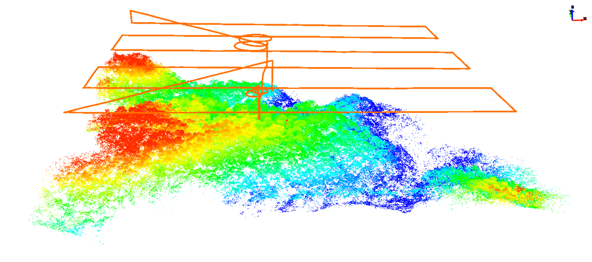
The DJI^® pilot software is employed to design the flight route and guide the flight of the UAVs. The flight mode of the two planes is designed for the same flight route so that a consistent measurement area can be obtained. It is worth noting that in forest areas, due to the dense layers of trees, there are significant risks during takeoff and landing, so it is usually necessary to find a suitable landing location. We usually choose the location at the “forest gap”, which is usually a tomb, ridge, or other natural bare ground. At the beginning of the takeoff phase, we manually operated the UAV to avoid trees near the forest gap to reduce the risk of a crash while completing inertial guidance for the IMU. After the takeoff reaches the specified height, it changes to automatic flight (as shown in Fig. 2).

Figure 2 Flight route of this study.

2.4 Lidar-based tree segmentation and canopy structure calculation

The study specifically uses GreenValley^® LiDAR360 and Esri^® ArcGIS software to carry out this part of the work. First, the laser point cloud results are coordinated and spliced, and then the noise is removed when it surpasses 5 times the standard deviation. After this the improved progressive triangulated irregular network (TIN) densification (IPTD) algorithm is used to separate the ground points (Zhao et al., 2016). On this basis, a digital elevation model is generated based on the inverse distance weight (IDW) method (Ismail et al., 2016).

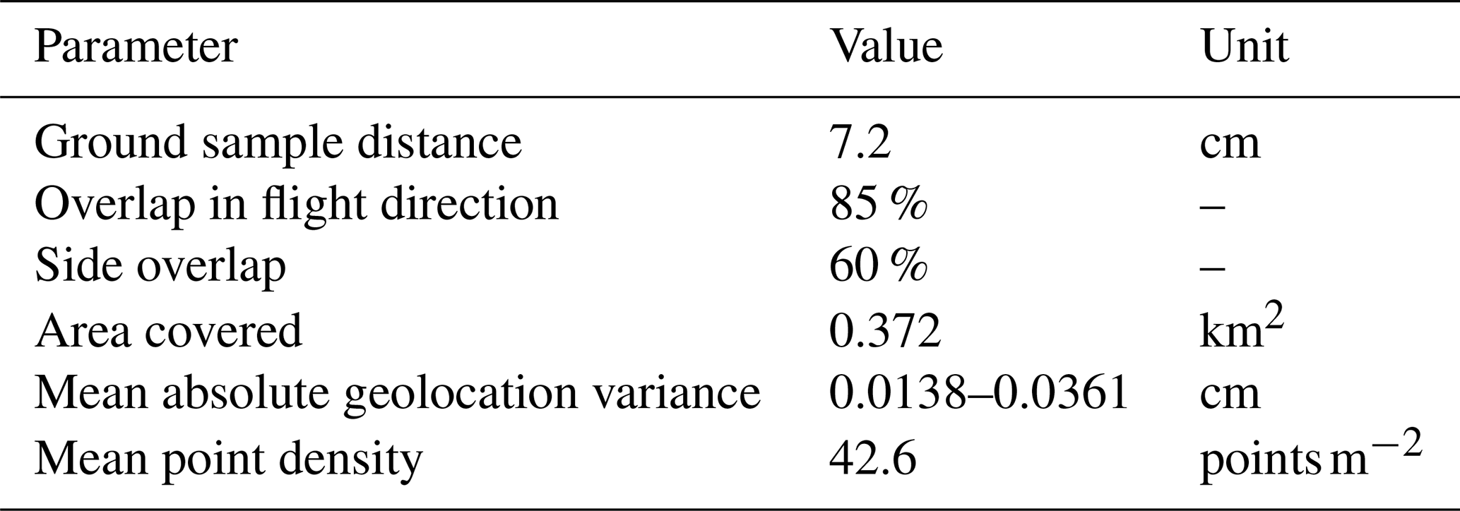
The processing of obtaining single-tree features based on lidar is based on the layer-stacking algorithm (Ayrey et al., 2017). According to the layer height of different trees, the position of the seed point in the laser point cloud is determined for segmentation, and then the boundary of each tree is obtained. The principle of this algorithm is to first obtain the seed points of each single tree and then find its watershed (Li et al., 2012). On this basis, the default calculation module of LiDAR360 is used to obtain the structural characteristic parameters of tree canopy, such as the canopy height and crown radius (Ma et al., 2017). At the same time, we fuse and concatenate the airborne visible-light image into image raster data. Based on the individual tree boundary, the results of the visible-light raster data segmentation through the overlay analysis of ArcGIS are used to obtain the raster of each individual tree. The specific parameter settings for airborne image data processing are shown in Table 1. After that, the raster of individual trees is given to different apps to obtain the plant species identification results.

Table 1 The specific parameter settings for airborne image data processing.

2.5 Vegetation identification

With the continuous improvement of a new generation of plant recognition algorithms based on deep learning methods, a variety of plant recognition apps and platforms continue to appear (Irimia et al., 2020; Otter et al., 2021). They can all import and identify plant images from mobile phones or communicate via an application programming interface (API) with public researchers. There are also quite a lot of open-source deep-learning-trained models and datasets, allowing for researchers to submit visible-light images and obtain recognition results (Ma et al., 2019; Zhanhui et al., 2020).

The apps and platforms shown in Table 2 were used in this study to identify the visible-light image after point cloud segmentation. They are usually trained based on a certain national or international plant classification picture database. For example, AiPlants^® is based on the database of the Plant Photo Bank of China (PPBC) (Zhanhui et al., 2020). With the rise of cloud computing services, individual calling methods on various platforms have arisen, such as the Aliyun^® general image recognition service (GIRS), Amazon^® Rekognition service, and Baidu^® PaddlePaddle platform. And their identification results can be obtained using a simple script submission (Jin, 2017). However, due to differences in their respective training sets, the accuracy of plant recognition varies among different apps. It is currently unclear whether the reliability, accuracy, and portability of these simple retrieval methods can support their application in investigating plant emissions. In this study, a simple method of recognition and judgment was adopted to ensure our recognition accuracy. We perform a conditional judgment on all results, and if one piece of input data obtains the same recognition result on two or more platforms, the recognition result is accepted.

Zhanhui et al. (2020)Jin (2017)Ma et al. (2019)Kumar et al. (2012)Joly et al. (2016)Otter et al. (2021)Mäyrä et al. (2021)

Table 2 List of plant species identification apps and platforms.

2.6 BVOC emission factor and emission calculation

In this study, calculations are based on the database of detailed BVOC emission factors (EFs) for tree species provided by MEGAN3.2, which contains a set of EF libraries with more than 40 000 tree species (Guenther et al., 2018). When the tree species determined based on Sect. 2.5 is clear, the corresponding BVOC EF can be obtained by lookup in the table.

For the types of trees that are not contained in the EF library, we obtain the BVOC emission factor of the tree species based on the literature survey method (Chen et al., 2022; Mu et al., 2022). For tree species that cannot be found even through literature research, we choose to replace them with plants from the same family. Because there are quite a few types of BVOCs obtained by observation experiments, they are generally dominated by isoprenes and monoterpenes (Li et al., 2021). Therefore, our study is also characterized by the distribution of emissions using a genus-specific average emission factor.

Since the images we use to identify tree species are singularly temporal, we only attempt to calculate the maximum and minimum emissions of the forest in the sample plot. The calculation method is based on the emission factors corresponding to the species of each tree multiplied by its biomass and the area occupied by its crown diameter.

3 Results

3.1 The morphological composition of the vegetation

Based on the point cloud results measured by lidar, more accurate arboreal morphological characteristics can be obtained. Then we split the individual trees, and the point clouds of each individual tree are shown in Fig. 3. It can be seen that due to the influence of terrain, the point cloud at the edge has a much lower density than the point cloud in the center, which may cause higher uncertainty in the segmentation of the single forest in this area.

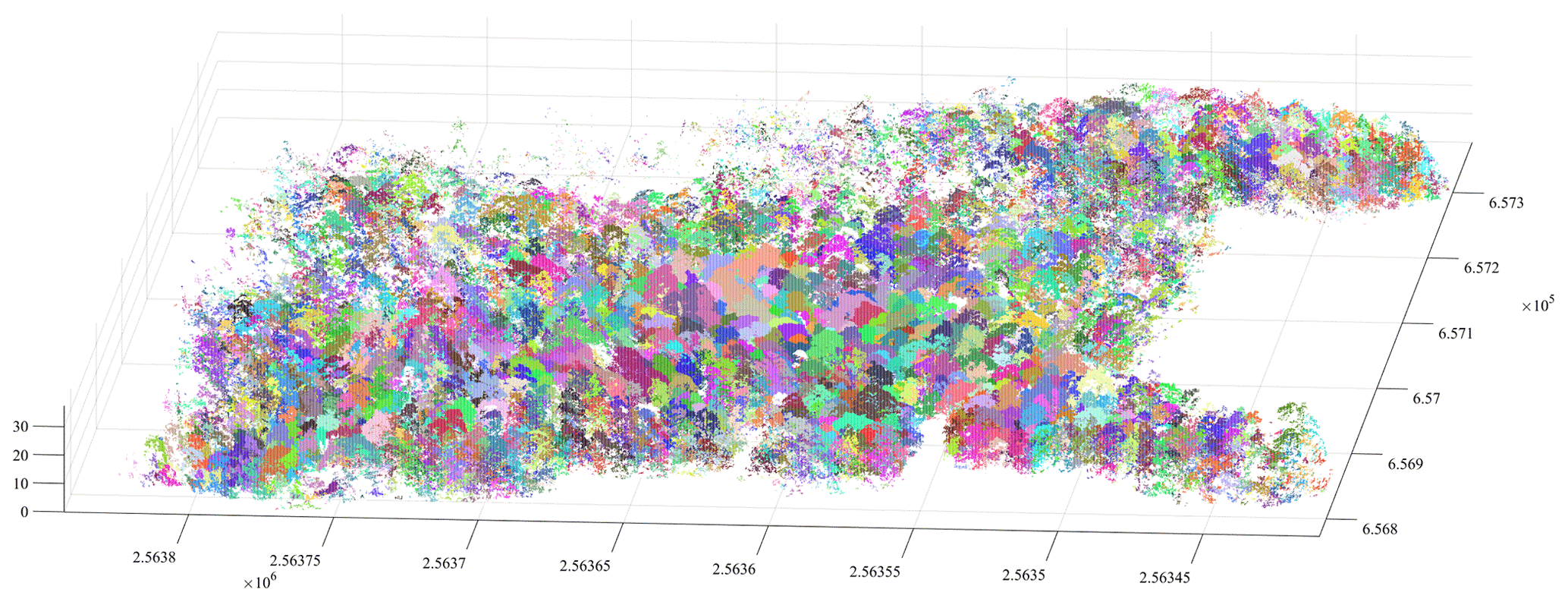
Figure 3 Point cloud of each individual tree obtained based on the layer-stacking algorithm excluding topographic.

After the statistics of single-tree segmentation, there are 1291 trees in the sample plot. The overall distribution of morphological parameters and the corresponding relationship between the tree height and crown diameter of each tree are shown in Fig. 4. It can be seen that the tree height in the sample plot obtained by the measurement follows the GaussAmp skew distribution. Its distribution range spans from 2 to 30 m, and its average is 14.9 m. At the same time, its crown radius presents a lognormal distribution, and its average value is about 4 m.

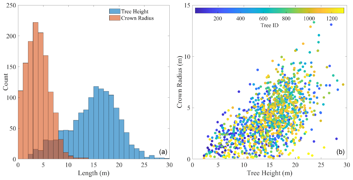
Figure 4 The distribution of tree height and crown radius: (a) overall distribution and (b) each tree.

3.2 The composition of vegetation species

The plant identification apps were called to identify the tree species based on the segmentation results. The spatial distribution and frequency of tree species are shown in Fig. 5 and Table 3. It can be seen from its spatial distribution that different tree species appear to be scattered and gathered. Among them, the three most frequent tree species are Aidia canthioides (Champ. ex Benth.) Masam., Macaranga sampsonii Hance, and Blastus cochinchinensis Lour., while the highest-frequency family is Euphorbiaceae. The ratio of the top three species is about 12 %, 11 %, and 6 %. Other identified tree species are also shown in Table 3. Combined with their canopy morphology distribution, it can be seen that the plot presents significant coniferous–broadleaved mixed-forest characteristics, and coniferous or broadleaved trees occupy the position of the dominant tree species. Meanwhile, it still can be see from Fig. 5 that lots of trees could not recognized.

Figure 5 The spatial distribution of tree species.

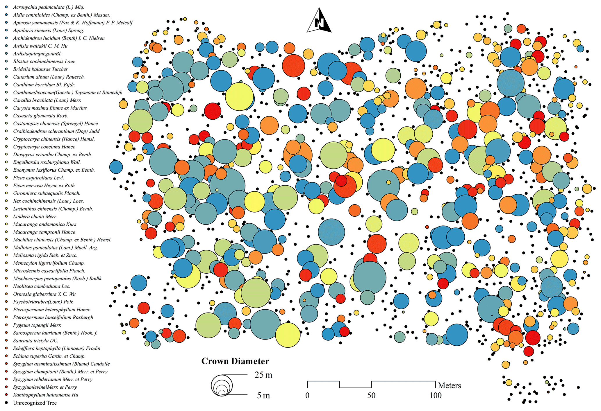
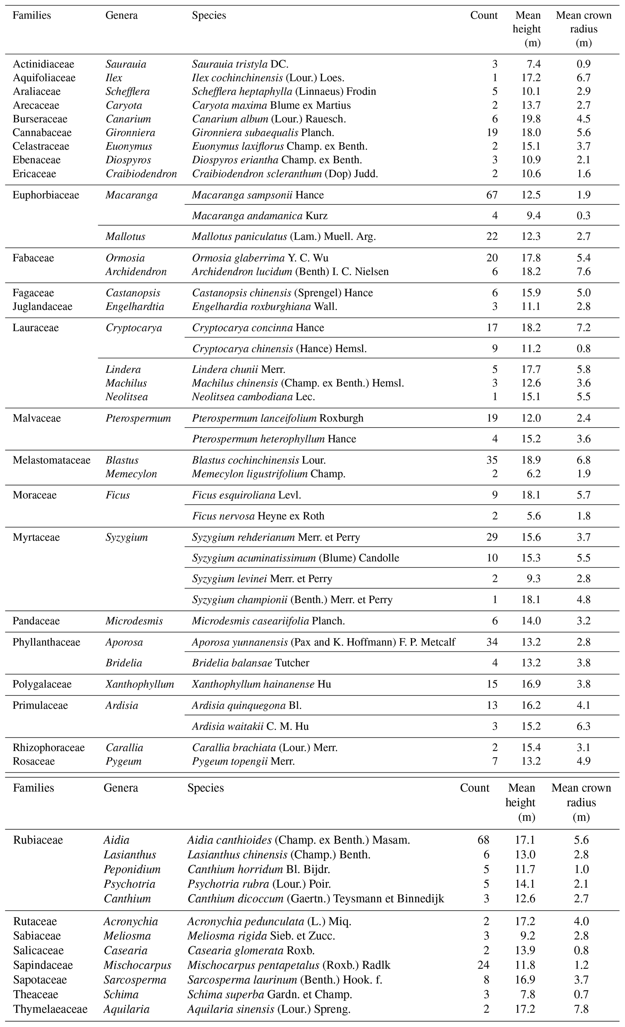
Table 3 Specific species composition information of the vegetation identification result.

3.3 The BVOC emission at the family and individual scale

The emissions we obtained for isoprenes and monoterpenes for each family are shown in Table 4. It can be seen that in the study area of Dinghu Mountain, the largest cumulative isoprene emissions were from the Myrtaceae family (maximum of 18.7 $\mathrm{\mu }\mathrm{g}\mathrm{C}{\mathrm{m}}^{-\mathrm{2}}{\mathrm{h}}^{-\mathrm{1}}$), followed by the Salicaceae family (maximum of 3.8 $\mathrm{\mu }\mathrm{g}\mathrm{C}{\mathrm{m}}^{-\mathrm{2}}{\mathrm{h}}^{-\mathrm{1}}$), while for monoterpenes their cumulative emissions were largest in the Rubiaceae family (maximum of 3.9 $\mathrm{\mu }\mathrm{g}\mathrm{C}{\mathrm{m}}^{-\mathrm{2}}{\mathrm{h}}^{-\mathrm{1}}$), followed by the Theaceae family (maximum of 2.8 $\mathrm{\mu }\mathrm{g}\mathrm{C}{\mathrm{m}}^{-\mathrm{2}}{\mathrm{h}}^{-\mathrm{1}}$). However, it is worth noting that since we cannot confirm the leaf type, leaf age, and corresponding phenological period of each tree, we only calculated the maximum and minimum possible emissions based on their standard emission factors and biomass.

Table 4 The maximum and minimum emissions from different families in the study area (unit: $\mathrm{\mu }\mathrm{g}\mathrm{C}{\mathrm{m}}^{-\mathrm{2}}{\mathrm{h}}^{-\mathrm{1}}$).

At the same time, the spatial distribution of individual plant emissions from Fig. 6 shows that there are clusters of BVOC-emitting plants in the study area, which are caused by the aggregation of plants of the same family. The clusters of isoprene- and terpene-emitting plants are homogeneous, while there are some non-BVOC-emitting plants between the different clusters, which may be related to their ecological-competition strategy (Fitzky et al., 2019). According to the forest competition theory, the emissions of BVOCs are related to its competitive pressure, relative size, and area overlap rate (Contreras et al., 2011). On the other hand, the strategies adopted by different species are different. The intra-specific competition and inter-specific competition play a specific role through different biopheromones, which are all BVOCs (Šimpraga et al., 2019). In addition, it is noteworthy from Fig. 6 that the number of plants not discriminated in the study area is quite large, implying that this is an important source of uncertainty in the estimation of BVOC emissions in this method.

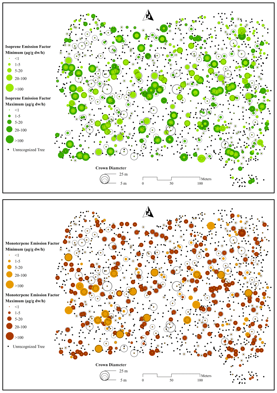
Figure 6 The individualized spatial distribution of the isoprene and monoterpene emission factor.

4 Discussion

4.1 The uncertainty sources of this method

4.1.1 Flight route design and acquisition process of aerial survey data

During the field flight using this workflow, we found that the height of the flight and the pixel area occupied by each tree in the resulting visible-light image is the decisive link that determines whether the image recognition tool can effectively identify the plant species in the image. In a practice flight, we designed different flight altitude routes, namely 60, 120, and 200 m, in order to find a suitable flight altitude. We checked and found that for the images obtained at a flying altitude of 120 m or more, the number of pixels per tree obtained after being cut and paired by a single tree in the lidar point cloud is less (about 200×300 pixels). The description of tree leaf characteristics is very unclear and presents mosaic-like characteristics, which makes it impossible to accurately identify hidden plant species in different image recognition tools and which also makes the calculation of BVOC emissions hard. Especially due to the fact that the images obtained from drone flight surveys are all orthophoto images, their expression in canopy morphology features is missing.

At the same time, the vegetation below the forest canopy also emits a considerable number of BVOCs. Although airborne lidar can detect their presence through leaf gaps, visible-light images cannot obtain their information due to canopy occlusion, making it an important source of underestimation of BVOC emissions for this method. It may be possible to try using lateral aerial photography or airborne multi-band enhanced penetrating lidar technology to achieve detection and modeling recognition of understory plants.

4.1.2 Single-tree segmentation and recognition process of images

The single-tree segmentation technique used in this study is based on the layer-stacking algorithm. This single-tree segmentation process first obtains the seed points of each tree and then determines the boundaries between each individual tree through its watershed (Li et al., 2012). This method may result in undetected or incorrectly detected trees, depending on the density of the laser point cloud per unit area. In this study, the density of laser point clouds was 42.6 points m⁻², which, although very high, may still result in some small saplings not being correctly identified. In future research, techniques such as ground-based lidar segmentation and coarse-to-fine algorithms can be combined to improve its accuracy (Zhao et al., 2023).

It also can be seen that the recognition accuracy of these apps is not as high as it claims for the visible-light images obtained by drones. Among them, platforms trained by satellite images give quite accurate results of tree species recognition. EasyDL gave back “unrecognizable” feedback for quite a lot of individual tree images, while AiPlants and Leafsnap gave incorrect classification and recognition results, such as succulents and garden plants. This result may related to the fact that the apps did not train on image inputs with correct tree species tags during the collection and training of the general image datasets.

In general, for the refined calculation of vegetation VOC emission factors, the platform based on deep learning training from remote sensing images can provide faster and more reliable tree species identification results than traditional methods. However, these recognition platforms still require more accurate and large-scale training datasets to support their classification accuracy. Although various crowdsourcing-based apps are widely used, most of the vegetation tree species information uploaded by users is concentrated in garden tree species or common tree species, and more sample images are needed for rare tree species. Due to the differences of functions and selected training datasets of different platforms, it is difficult to quantify the range of uncertainty of this process. With the development of open-source databases and open-source training sets, further uncertainty source control of this process can be promoted.

Guenther et al. (2012)Gao et al. (2011)Situ et al. (2013)Tang et al. (2007)Wu et al. (2016)Li et al. (2021)

Table 5 Measurements and simulations of isoprene and monoterpene emissions or concentrations using different methods at the same site. REA: relaxed eddy accumulation, GC–MS: gas chromatography–mass spectrometry .

4.1.3 The estimation process of BVOC emissions

Although this study integrated MEGAN's emission tree species information and literature obtained information as input calculations, MEGAN mainly consists of common tree species at the global scale. Therefore, the emission factors of various tree species used in this study mainly came from the Mu et al. (2022) database of measured results. This has made it quite difficult to measure over a hundred species of trees in southern China, allowing for the discovery of emission factor information for most of the tree species in the sample plot of this study. But this situation indicates that there are several technical issues in selecting the BVOC emission factor library when applying this framework. Firstly, there is still a considerable number of cases in this study where the tree species analyzed is not within the range of the MEGAN EF database. Secondly, the emissions of BVOCs from trees are subject to various photochemical and hydrothermal conditions, but, currently, various databases are unable to provide a detailed characterization of the impact of these environmental factors at the tree species level. Thirdly, different BVOC emission factor databases have a different emphasis on the emission parameters of BVOC components for the same tree species. The shortcomings above limit our further application and migration of this method to other forests. However, this method can quickly obtain an independent set of upper and lower limits of BVOC emissions for its sample plot, which is helpful for conducting model validation work based on the sample plot. It is recommended that community peers refer to our workflow and combine it with their local tree species emission factor library to further BVOC emission estimation.

Meanwhile, it is important for the academic community to understand that existing BVOC computational emission models such as MEGAN have already taken into account various meteorological conditions, leaf growth, and other factors relatively completely. However, the definition of vegetation itself often depends on the definition of land use types in the coupled regional models. For example, in the commonly used WRF-Chem (Weather Research and Forecasting) model, vegetation types are usually classified using the MODIS 20 or USGS 24 classification systems, which still use a combination of coniferous forests, broadleaved forests, mixed forests, evergreen forests, and deciduous forests for forest classification. This means that there is a need for further improvement in the characterization of emissions from different tree species. Therefore, future regional estimation of BVOCs can be carried out by combining the method framework obtained in this study with the coupling of BVOC computational emission models.

4.2 The differences in BVOC emission from other methods and potential impact

We compared the BVOC results obtained in this study with the emission results obtained by different methods in the Dinghu Mountain sample plot, as shown in Table 5. It can be seen that there are many different research methods (including remote sensing inversion, model calculation, understory sampling observation, UAV-mounted sensor observation), and the magnitude of the BVOC emissions from Dinghu Mountain varies greatly. The results obtained from this study indicate that a more accurate description of forest biodiversity can make the calculated results more consistent with those obtained from direct observations in the forest canopy. At the same time, it has been found that in previous model estimations based on simple plant functional type (PFT) methods to estimate biomass, the emissions of BVOCs may be underestimated to a considerable extent. This poses new requirements for the estimation and parameterization of BVOC emissions; that is, when simulating the emissions of BVOCs, the biodiversity of the forest in the region should be considered and not only vegetation factors from purely canopy physical size indicators such as leaf area index (LAI) and crown diameter.

5 Conclusions

This research has established a workflow for identifying plant species based on lidar, photogrammetry, and image recognition technologies carried by drones to obtain accurate BVOC emissions. The intention of this research is to combine the newly developed rapid survey method of plant species with the calculation of BVOC emissions and discuss the main uncertainty sources of the BVOC emissions obtained in this method. The current limitation of this study is that although lidar can capture the multi-layer structure of tree crowns, visible light is difficult to identify other vegetation below trees, such as shrubs and herbs, which can result in a certain loss of BVOC emissions.

The implication of this study is that, with the advancement of novel technologies in computer science, the obstacle of tree species identification, which previously impeded the estimation of BVOC emissions, will gradually be addressed through large-scale image recognition technology. However, open-source and standardized image recognition techniques, along with the BVOC emission factor library for tree species, have emerged as new bottlenecks, necessitating the relevant research community to contemplate how to share corresponding data and technologies more openly.