A multi-instrument fuzzy logic boundary-layer-top detection algorithm

Understanding the boundary-layer height and its dynamics is crucial for a wide array of applications spanning various fields. Accurate identification of the boundary-layer top contributes to improved air quality predictions, pollutant transport assessments, and enhanced numerical weather prediction through parameterization and assimilation techniques. Despite its significance, defining and observing the boundary-layer top remain challenging. Existing methods of estimating the boundary-layer height encompass radiosonde-based methods, radar-based retrievals, and more. As emerging boundary-layer observation platforms emerge, it is useful to reevaluate the efficacy of existing boundary-layer-top detection methods and explore new ones.

This study introduces a fuzzy logic algorithm that leverages the synergy of multiple remote sensing boundary-layer profiling instruments: a Doppler lidar, infrared spectrometer, and microwave radiometer. By harnessing the distinct advantages of each sensing platform, the proposed method enables accurate boundary-layer height estimation both during daytime and nocturnal conditions. The algorithm is benchmarked against radiosonde-derived boundary-layer-top estimates obtained from balloon launches across diverse locations in Wisconsin, Oklahoma, and Louisiana during summer and fall. The findings reveal notable similarities between the results produced by the proposed fuzzy logic algorithm and traditional radiosonde-based approaches. However, this study delves into the nuanced differences in their behavior, providing insightful analyses about the underlying causes of the observed discrepancies. While developed with the three instruments mentioned above, the fuzzy logic boundary-layer-top detection algorithm, called BLISS-FL, could be adapted for other wind and thermodynamic profilers. BLISS-FL is released publicly, fostering collaboration and advancement within the research community.

1 Introduction

The atmospheric or planetary boundary layer (BL) is often defined as the layer of the atmosphere directly influenced by Earth's surface. This is the portion of the atmosphere where the bulk of human socioeconomic activity takes place, yet it is also one of the least routinely observed portions of the atmosphere. Given the depth of the atmosphere and common obfuscation by clouds (e.g., McGrath-Spangler and Denning, 2013), satellite-based observing of the BL remains difficult and uncertain. Commonly and consistently available observations include surface meteorological conditions and weather radar observations, which both may provide indirect inferences about BL conditions. The only widely available direct observations of the BL in the United States are radiosondes, which are typically only launched twice per day at 00:00 and 12:00 UTC (European nations, for example, have developed a diverse network of lower-atmospheric sensors; see, e.g., Cimini et al., 2020; Rüfenacht et al., 2021). Operational radiosonde sites are spaced at best hundreds of kilometers apart (Melnikov et al., 2011), which is insufficient for representing conditions on mesoscales to BL scales. This lack of observation in the BL has been coined a “data gap” (Bell et al., 2020), and several community reports and surveys have long called for improvement (National Research Council, 2009, 2010; National Academies of Sciences, Engineering, and Medicine, 2018a, b) to serve the diverse socioeconomic needs of modern society.

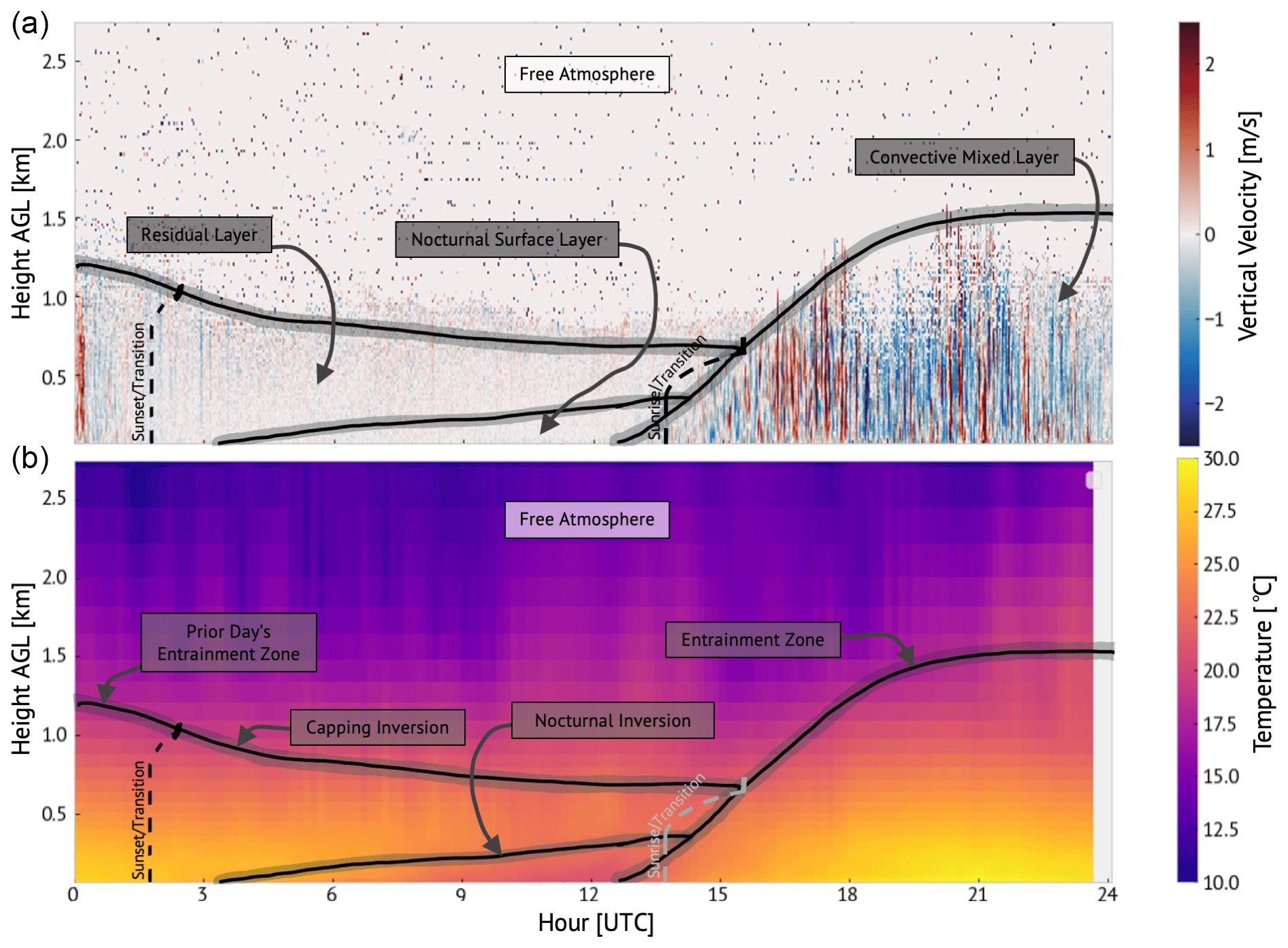
The BL evolves on a diurnal cycle, as shown in Fig. 1. As the sun rises (depicted as occurring shortly after 12:00 UTC in Fig. 1) the Earth's surface is warmed, which through heat (and moisture) fluxes leads to turbulence processes that mix the atmosphere above the surface. As these processes continue and grow, the well-mixed region above the surface becomes deeper, developing the BL. The entrainment zone separates the BL from the free atmosphere and is characterized by transfer of mass and momentum across this boundary. The BL height continues to increase throughout the day as the convective mixed layer grows (barring disruption by other forcing such as an air mass change or strong advection) until the sun begins to set (depicted as occurring near 01:30 UTC in Fig. 1). The evening transition is characterized by the decay of the previous day's turbulent mixing. As mixing slowly shuts down and the surface loses heat to the atmosphere, the surface typically becomes cooler than the atmosphere above it, setting up a shallow surface-based inversion. This marks the beginning of the nocturnal BL or nocturnal surface layer. Above this layer, the residual layer retains characteristics of the previous day's boundary layer and is topped with the capping inversion (remnants of the entrainment zone). In conditions that allow for continued cooling, the nocturnal surface layer grows until the sun rises again, repeating the process on another day.

Figure 1 A conceptual diagram of the diurnal BL cycle, as often adapted from Stull (1988), overlaid on observed vertical velocity (a) and temperature (b).

Knowledge of the BL height and its evolution is central to many high-impact applications. These include air quality transport and dispersion forecasts (e.g., Dabberdt et al., 2004), fire weather monitoring and evolution (e.g., Clements et al., 2007), and the initiation of deep moist convection (e.g., Browning, 2007). Additionally, as numerical weather prediction models play an increasingly large role in the forecast process, real-world BL height observations are crucial for constraining planetary BL parameterization schemes (e.g., Cohen et al., 2015), which can have a pronounced effect on subsequent convection forecasts (e.g., Crook, 1996; Stensrud and Weiss, 2002; Cohen et al., 2017) but have been shown to often exhibit large errors compared to observations (e.g., Grimsdell and Angevine, 1998). Recently, Tangborn et al. (2021) found the accuracy of the temperature and wind fields in the simulated afternoon convective BL to be improved compared to radiosonde observations when assimilating observations of BL height.

A variety of observation platforms are used to measure BL processes. For example, Doppler radar at various wavelengths (Gal-Chen and Kropfli, 1984; Minda et al., 2010; Banghoff et al., 2018; Duncan et al., 2019), radar wind profilers (e.g., Ecklund et al., 1988; Rogers et al., 1993), microwave radiometers (e.g., Troitsky et al., 1993; Djalalova et al., 2022) and interferometers (e.g., Feltz et al., 1998; Knuteson et al., 2004; Turner and Löhnert, 2014), lidar-based instruments (e.g., Grund et al., 2001; Froidevaux et al., 2013; Spuler et al., 2021), spaceborne platforms (e.g., McGrath-Spangler and Denning, 2012), instrumented towers (e.g., Fernando et al., 2019), and both piloted (e.g., Hane et al., 1993) and unpiloted (Segales et al., 2020) aircraft are all common tools used to understand the BL and its structure and processes. Myriad methods exist specifically for deducing BL height. Estimation based on data from balloon-borne radiosondes is one widely used method (Seidel et al., 2010). Seemingly straightforward, this method has drawbacks such as poor spatial resolution, as discussed previously, and discrepancies between the exact profile techniques used to find the BL height. Ceilometers are often integrated into Automated Surface Observing System (ASOS; NOAA et al., 1998) stations in addition to common deployment for research purposes (e.g., Uzan et al., 2016). Aerosol backscatter as measured by ceilometers can be used in various techniques – some provided by instrument manufacturers, some developed by operators – to estimate BL height (Caicedo et al., 2017). Even within one manufacturer-provided method, BL height estimates can be ambiguous and require additional analysis, as Caicedo et al. (2017) found with the CL31 ceilometer. Radar wind profilers can provide multiple products from a single platform, which have been combined in fuzzy logic algorithms to estimate BL height (Bianco and Wilczak, 2002, 2008). This approach demonstrates how combining multiple measurements including those of processes indirectly related to BL height may be useful in an estimation technique. However, radar wind profilers typically do not have very high temporal resolution and are not as small in form factor as some other BL observation platforms such as lidars.

Bonin et al. (2018) proposed a fuzzy logic algorithm for determining BL height from Doppler lidar data and found promising results using data from the Indianapolis Flux Experiment (INFLUX; Davis et al., 2017). As an aside, Bonin et al. (2018) use the term mixing-layer height or mixing height, not BL height. Their terminology choice makes sense as their analysis and algorithm are limited to only lidar data and thus only evaluate mechanical mixing processes in the boundary layer. However, we use the term BL height throughout this work, expecting that it is inclusive of (but not limited to) mixing processes. The approach laid out by Bonin et al. (2018) is advantageous in that it combines multiple estimates of BL height, provides a measure of uncertainty for each estimate, and is adaptable to users' individual needs and cases. However, no thermodynamic information is incorporated. In a review of BL height detection approaches, Kotthaus et al. (2023) specifically described the potential benefits of instrument synergy for a variety of applications. We hypothesize that, similar to the suggestions made in Kotthaus et al. (2023), the capability and applicability of a BL height estimation method (in the present case, a fuzzy logic algorithm) could be expanded by incorporating multiple instrument data streams.

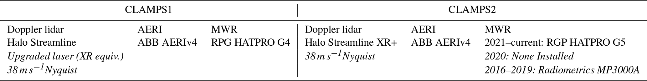
In recent decades several integrated platforms and sites have been developed, which combine BL thermodynamic and kinematic profiling capabilities such as the Department of Energy Atmospheric Radiation Measurement Southern Great Plains site (Sisterson et al., 2016) and multiple mobile facilities (e.g., Karan and Knupp, 2006; Knupp et al., 2009; Wingo and Knupp, 2015; Wagner et al., 2019). A team of scientists at The University of Oklahoma (OU) and NOAA's National Severe Storms Laboratory (NSSL) developed and continue to operate the Collaborative Lower Atmospheric Mobile Profiling Systems (CLAMPS1 and CLAMPS2). Designed as sibling platforms, OU-NSSL CLAMPS1 and NOAA-NSSL CLAMPS2 combine a Doppler lidar (DL), atmospheric emitted radiance interferometer (AERI), and microwave radiometer (MWR) into a single facility (see Table 1) capable of profiling temperature, moisture, horizontal wind, and vertical velocity with vertical resolution on the order of tens of meters and temporal resolution on the order of seconds to minutes (depending on the quantity of interest). Such integrated platforms provide a unique opportunity to explore multi-instrument value-added products. In the case of CLAMPS, these value-added products have the benefit of high temporal resolution, which can be critical for some applications. Recognizing the variability and strengths and weaknesses of various remote sensing BL height detection methods, we propose using the instruments on board CLAMPS together in a fuzzy logic approach for BL height estimation including thermodynamic BL profiles, which should allow this approach to operate in the overnight hours in at least some conditions. Herein, we expand from the work of Bonin et al. (2018) and introduce a new multi-instrument BL height detection algorithm.

Table 1 The three core instruments on board each CLAMPS facility are listed. For each instrument the listing includes the manufacturer, instrument model, and any additional notes (in italics) about specific instrument properties or history.​​​​​​​

2 Fuzzy logic algorithm

Fuzzy logic methods are used to discern and classify signals based on some known characteristics (Mendel, 1995). Fuzzy logic is unlike Boolean logic in that is allows for degrees of “truth” as opposed to the binary “true” or “false”. The fuzzy logic process relates input variables to an output characteristic via so-called membership functions, which vary from zero (which indicates the input variable is not a member of a given class) to 1 (which indicates the input variable is a member of a given class). By taking a weighted mean, the membership values of all input variables are aggregated and then defuzzified to determine the desired characteristic of the measurement.

Fuzzy logic methods were applied in many ways within atmospheric science before the work of Bonin et al. (2018). These approaches have been popular amongst radar scientists and developers, where it has been applied for identification of non-precipitation echoes and radar artifacts (Gourley et al., 2007; Mahale et al., 2014), hydrometeor classification methods (Vivekanandan et al., 1999; Liu and Chandrasekar, 2000; Park et al., 2009), and detection of precipitation modes (Yang et al., 2013). Applying the method to Doppler lidar measurements was a novel component of the Bonin et al. (2018) work. Our proposed algorithm uses fuzzy logic to combine high-resolution boundary-layer profiler observations from multiple instruments toward the goal of multi-method or multi-instrument synergy as described by Kotthaus et al. (2023).

We now describe and demonstrate our newly developed algorithm using CLAMPS1 observations collected in Norman, Oklahoma, on 25 June 2020, shown in Fig. 2. Much of the initial framework closely follows that of Bonin et al. (2018, hereafter B18), with any deviations from or expansions upon B18 highlighted. The fuzzy logic algorithm takes a two-step approach: a first-generation BL height estimate and a second-generation BL height estimate. In the first-generation step, only measurements of BL mixing processes (i.e., measurements that show mixing is ongoing) are included. Given the instruments available on CLAMPS, these measurements include turbulence information from the DL. The second-generation estimate additionally includes indicators of mixing processes (i.e., measurements that show that mixing has occurred). For example, a well-mixed potential temperature profile from the CLAMPS thermodynamic profilers would indicate BL mixing has occurred.

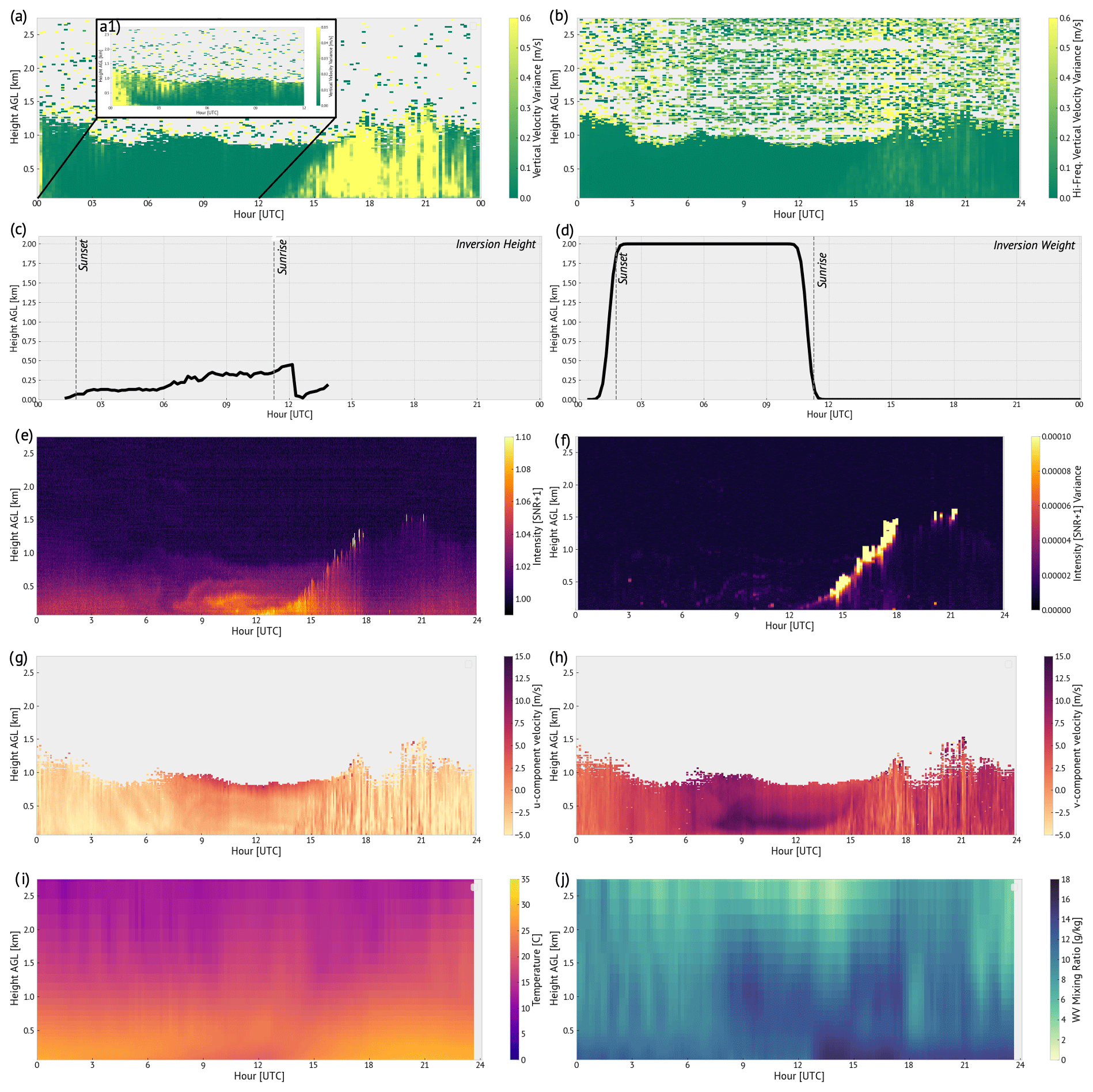
Figure 2 Time–height cross-sections showing the diurnal evolution of CLAMPS1 observations collected on 25 June 2020 in Norman, Oklahoma, which are used in the fuzzy logic algorithm to produce the aggregate fields and BL height estimates shown in Fig. 3. Panels (a)–(c) show the variables used in the first-generation step of the fuzzy logic algorithm (a: vertical velocity variance, b: high-frequency vertical velocity variance, c: temperature inversion height), with the weighting given to panel (c) shown in panel (d) based on sunrise and sunset time, while panels (e)–(j) show the variables used in the second-generation step of the fuzzy logic algorithm (e: backscatter intensity, f: backscatter intensity variance, g: u wind, h: v wind, i: temperature, j: water vapor mixing ratio). Panel (a) includes a subsetted window (a1) between 00:00 and 12:00 UTC with a finer color scale to show overnight values of vertical velocity variance. Each observed field is labeled with units (if applicable) on its respective panel color bar.

In the first-generation step, vertical velocity variance, $\stackrel{\mathrm{‾}}{w^{\prime \mathrm{2}}}$ (Fig. 2a, a1), as computed from the DL vertical stare observations, and the high-frequency vertical velocity variance, $\stackrel{\mathrm{‾}}{w_{\text{HF}}^{\prime \mathrm{2}}}$ (Fig. 2b), are included as the indicator variables. The method for computing $\stackrel{\mathrm{‾}}{w_{\text{HF}}^{\prime \mathrm{2}}}$ is detailed in B18. It is computed in the same manner as $\stackrel{\mathrm{‾}}{w^{\prime \mathrm{2}}}$, except a high-pass filter is applied using a frequency of 0.0167 Hz as a threshold (i.e., periods less than 1 min) before evaluating the variance only at the remaining high frequencies. We apply it here to control for any potential contribution to vertical velocity variance signals due to non-turbulent motions such as waves, drainage flows, and sub-mesoscale motions (Bonin et al., 2017). B18 include several other variables from the more complex Doppler lidar scan patterns available in their dataset; we include only $\stackrel{\mathrm{‾}}{w^{\prime \mathrm{2}}}$ and $\stackrel{\mathrm{‾}}{w_{\text{HF}}^{\prime \mathrm{2}}}$ as indicators. The membership functions are defined as half-trapezoids following B18, where parameters x₁ and x₂ are the values at which the function increases above zero and reaches a maximum of 1, respectively. For $\stackrel{\mathrm{‾}}{w^{\prime \mathrm{2}}}$, x₁=0.02 and x₂ = 0.08 m² s⁻². For $\stackrel{\mathrm{‾}}{w_{\text{HF}}^{\prime \mathrm{2}}}$, x₁=0.0025 and x₂ = 0.01 m² s⁻². In the fuzzification step, data are re-gridded via interpolation onto a common 10 m by 10 min grid and evaluated via the membership function, becoming a standard shaped field of values from zero to 1 reflecting degree of membership in the BL. Both input variables are given equal weights of 1.

At this stage the algorithm design deviates from the design of B18. Since the first-generation estimate depends only on measures of mixing, it relies only on mechanically induced turbulence and mixing to determine BL height. Buoyancy-driven processes also play a role in BL development and are often a dominant process at night when stable boundary layers are more common. In later steps the BL height estimate from the first-generation step is used as a type of constraint on the second-generation step. Thus if there is a complete failure to detect a BL height (presumably in situations in which the BL depth is driven by buoyancy instead of mechanically driven processes) in the first-generation step, the second-generation step is unable to recover. In order to capitalize on the availability of thermodynamic profiles and to improve the capability and robustness of our algorithm during nocturnal hours when the mechanical mixing that backscatter-based instruments (e.g., Doppler lidar) observe can be absent or limited to the residual layer (Schween et al., 2014), the first-generation step also includes temperature inversion height (Fig. 2c) as an input variable (note: this is not a measure of mixing). To limit the effect of this additional input beyond periods where buoyancy-driven processes are more likely to dominate mechanical generation of mixing (e.g., nocturnal stable periods), a time-dependent weighting function is defined based on the local sunrise and sunset time (Fig. 2d). This weighting function allows the inversion height to have an effect on the algorithm during the overnight hours with sloped increasing and decreasing weights during the evening and morning transitions, respectively. The membership function in this case is stepwise and thus not authentically a fuzzified field. All levels above and below the inversion height are assigned membership values of zero and 1, respectively.

Now that all the first-generation variables are in place, they are aggregated together by taking a weighted mean. Recall that $\stackrel{\mathrm{‾}}{w^{\prime \mathrm{2}}}$ and $\stackrel{\mathrm{‾}}{w_{\text{HF}}^{\prime \mathrm{2}}}$ are both assigned a weight of 1. The inversion height has a time-variable weight ranging from zero during the day to 2 during the night. The result is one aggregate field representing the degree of membership in the BL based on these input variables. For our example case (Fig. 2), the first-generation aggregate is shown in Fig. 3a.

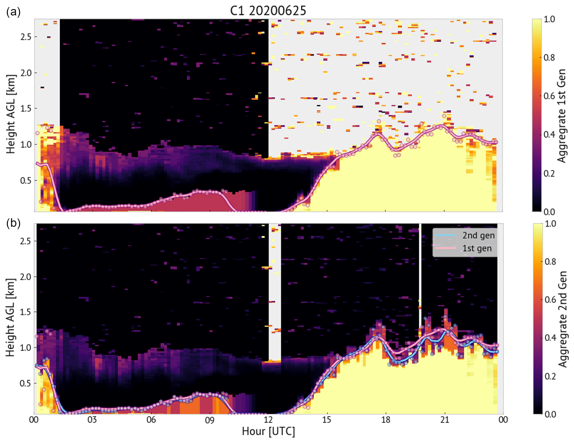
Figure 3 Fuzzy logic aggregate fields from the first-generation (a) and second-generation (b) steps of the algorithm. BL height estimates are traced on top of the color-fill aggregate values. Circles show BL height estimates which are computed every 10 min, while the curve shows the smoothed estimate after passing through a triangle weighting function.

The top of the boundary layer is defined as the first level where the aggregate value is less than or equal to 0.5, following B18. Using only the first layer where this condition is met guarantees the identified level is connected to the surface and not an elevated layer. Using the above-described definitions and constraints, the first-generation estimates of the boundary-layer top are compiled. These values will be used in the second-generation step as constraints within the fuzzy membership functions.

In the second-generation step, profiles of signal-to-noise ratio (SNR) (Fig. 2f), SNR variance (Fig. 2e), u-component wind (Fig. 2g), and v-component wind (Fig. 2h) from the Doppler lidar are all used, consistent with B18. This algorithm also includes information from CLAMPS thermodynamic retrievals in the form of potential temperature (Fig. 2i) and water vapor profiles (Fig. 2j). For all of these profiles, this algorithm dynamically defines the membership function for each profile (each time an observation is available) using the same approach as B18; all profiles are passed through a discrete Haar (Haar, 1910) wavelet transform to detect gradients, and membership is defined based on those gradients. The use of Haar wavelets to identify gradients in lidar backscatter is not new (e.g., Cohn and Angevine, 2000; Davis et al., 2000; Brooks, 2003); we extend the approach to thermodynamic profiles here.

For each profile considered, a discrete Haar wavelet transform is applied to the profile at each time. The sensitivity of the Haar wavelet dilation was examined and determined to be low in this application; a default value of 100 m was used here. In the case of u- and v-component profiles, the transform is applied to each profile separately, and then the vector magnitude of the wavelet transform is used in the membership function computation process to follow, following B18. In all cases, after the transform is applied the five peaks of greatest magnitude are identified. The height of each of those peaks is evaluated against the height of the first-generation boundary-layer-top estimate. Only peaks within 25 % of that estimate are retained (i.e., the aforementioned constraint). The membership function is then defined based on the remaining peaks:

$$\begin{array}{}\text{(1)}& M\left(z\right)=\left\{\begin{array}{ll}\mathrm{1},& z\le z_{\min }\\ \mathrm{1}-\frac{{\int }_{z_{\min }}^{z}P\left(z\right)\mathrm{d}z}{{\int }_{z_{\min }}^{z_{\max }}P\left(z\right)\mathrm{d}z},& z_{\min }<z\le z_{\max }\\ \mathrm{0},& z>z_{\max }\end{array},\right.\end{array}$$

where M is the membership function, P is the profile of peak magnitudes, and z is height above the surface. Since only select peaks are retained, P is nonzero only at the heights of retained peaks. In this notation, z_min and z_max are the heights where the lowest and highest peaks occur, respectively. If no peaks are identified, then no membership function is generated for the given input and it is not included in the aggregate at that time. This method of defining the membership function is considered dynamic since it is repeated for each unique profile, allowing it to change as a function of time.

The second-generation aggregate is produced like the first – by employing a weighted mean. As mentioned previously, the membership values from the first-generation step are included in this mean with a weight of 1 (except the inversion height; the time-varying weight still applies). Second-generation variables are all given a weight of 2. Again, the first level where the aggregate value is less than or equal to 0.5 is used as the threshold to define the boundary-layer top. The complete fuzzy-logic-based BL-top detection algorithm is summarized in flowchart form in Fig. 4. The second-generation estimate of boundary-layer top is the final estimate and is shown for the example case in Fig. 3b.

Figure 4 A flowchart visualization of the fuzzy logic algorithm steps used to detect boundary-layer height using multiple instruments on board the CLAMPS platform.

Since all data were fuzzified onto a common 10 min by 10 m grid, fuzzy logic boundary-layer-top estimates are provided every 10 min. Given that we know the BL grows and decays as a physical process, we can use information about the points surrounding a given point to both smooth extreme variability in the estimate (which could arise as artifacts of observation or algorithm limitations) and provide a measure of that variability for users. A centered triangle window method (with a width of 1 h) is applied to the 10 min estimates of BL height. Using triangle weighting, a weighted mean is used to smooth the BL height estimates in time. To preserve information about variability, all samples within the centered window are included to compute a standard deviation representative of that mean. The centered triangle window slides from sample to sample, retaining the 10 min resolution of the provided dataset. The provided output also provides data on a centered hourly time axis for a more simple comparison to standard observation platforms such as radar wind profilers, ceilometers, and radiosondes, which are more often available precisely on the hour.

In the case shown in Fig. 2 (and in the CLAMPS datasets described next in Sect. 3), care was taken to understand how the instruments operated, as well as any quality assurance applied to the data during their initial collection and production, and to determine if any additional quality assurance was needed before providing the data to the fuzzy logic algorithm. The CLAMPS platform happens to be a highly automated system which applies a high level of quality assurance automatically, reducing (but not removing) user needs to further quality-assure CLAMPS datasets. This may not always be the case, and users must understand the potential impacts data quality may or may not have when providing inputs to any algorithm. In the case of our fuzzy logic approach, the physically based definition of membership functions limits in the first-generation step and the BL height-range constraint in the second-generation step both provide some safeguard against entirely artificial or problematic data, but ultimately users must consider the data quality provided to the algorithm when weighing the quality of BL height estimates.

3 Data

To understand the potential value of our algorithm combining high-resolution boundary-layer profiler observations from multiple instruments, it is critical that we examine the algorithm's output in comparison to reference data. Radiosonde observations are a commonly available and known source of data that can be used to estimate BL height, though not without uncertainty (Seidel et al., 2010; Kotthaus et al., 2023). This uncertainty is explored in order to provide a reference dataset for comparison to the proposed fuzzy logic algorithm for BL height. Three observation periods during which CLAMPS observations and radiosonde data are available concurrently are used.

3.1 CHEESEHEAD (2019)

The Chequamegon Heterogeneous Ecosystem Energy-balance Study Enabled by a High-density Extensive Array of Detectors (CHEESEHEAD) experiment was conducted near Falls Park, Wisconsin, in midsummer to early fall 2019 (Butterworth et al., 2021). Primarily sponsored by the National Science Foundation, additional support from NOAA enabled the concurrent deployment of CLAMPS1 and CLAMPS2 at Lakeland and Prentice airports, respectively, for approximately 5 weeks of data collection. CHEESEHEAD also included radiosonde launches near the WLEF-TV 400 m very tall tower site, which was approximately 45 km away from both CLAMPS locations (north of Prentice, west of Lakeland). The analysis presented in this work will focus on CHEESEHEAD observations collected from 19 September to 10 October 2019.

The CLAMPS1 (located at Lakeland Airport; 45.92° N, 89.73° W) DL collected plan position indicator (PPI) scans at 70° elevation every 20 min and remained in a zenith-pointing mode otherwise. The DL provides range-resolved, line-of-sight measurements of radial velocity, intensity (signal-to-noise ratio (SNR) + 1), and attenuated backscatter. In the case of PPI scans meant for velocity azimuthal display (VAD) analysis, these data are post-processed to produce profiles of horizontal wind speed and direction. The zenith-pointing scans are used for vertical velocity information and are post-processed to provide turbulence information such as vertical velocity variance. The DL was configured to provide profiles with 18 m vertical spacing. The CLAMPS1 MWR and AERI were both deployed, and thermodynamic profiles as retrieved by the TROPoe physically based algorithm (previous versions known as AERIoe; Turner and Löhnert, 2014) were made available every 10 min. For different user needs and use cases we provided retrievals using only AERI data, only MWR data, and combining the data from both the AERI and the MWR in the TROPoe retrieval algorithm. In this study we use the combined AERI + MWR thermodynamic retrievals.

The CLAMPS2 facility (located at Prentice Airport; 45.54° N, 90.28° W) operated similarly, but the DL collected PPIs at 60° elevation every 5 min. The onboard MWR was deployed similarly, but CLAMPS2's AERI was damaged in transit and did not operate for CHEESEHEAD. As such, CLAMPS2 retrievals are limited to MWR only. For the analysis presented herein, we chose to exclude CLAMPS2 CHEESEHEAD data from this analysis in order to remove any potential differences resulting from data sources, as it would have otherwise been the only non-AERI-based thermodynamic data source.

3.2 NWC/RIL (2020)

By summer 2020, planned CLAMPS field missions were canceled due to the 2019 global SARS-CoV pandemic. Under the uncertainty of when those missions may resume or be rescheduled, a local deployment was organized between the National Weather Center (NWC) and Radar Innovation Lab (RIL) properties in Norman, OK, to evaluate instrument readiness (near 35.1816° N, 97.4398° W). This deployment included the CLAMPS1 platform, which operated from 4 June–8 August 2020. This deployment location is within a short walk of the Norman, Oklahoma, National Weather Service upper-air release point. The DL conducted 70° elevation PPI scans, providing horizontal wind profiles every 5 min, and operated in vertical stare mode at all other times. The thermodynamic retrieval algorithm included both AERI and MWR observations; profiles are available every 10 min.

3.3 PBLTops (2020)

As part of an experiment seeking to develop this method and validate the dual-polarization radar-based boundary-layer detection method proposed in Banghoff et al. (2018), both CLAMPS platforms were deployed and continuously collected data from 21 August 2020 until 24 September 2020. During this period, CLAMPS2 remained stationary at The University of Oklahoma's North Campus (35.237° N, 97.463° W), 6.7 km north-northwest of the Norman, Oklahoma, National Weather Service (OUN) upper-air release point. In contrast, CLAMPS1 was deployed at the Kessler Atmospheric and Ecological Field Station (KAEFS; 34.984° N, 97.516° W), 29.6 km south-southwest of the CLAMPS2 site, from 21 August until 3 September 2020; for the remainder of the period, CLAMPS1 was deployed at the Shreveport National Weather Service Office in Shreveport, Louisiana (SHV; 32.452° N, 93.842° W), with collocated radiosonde launches. For both CLAMPS platforms, the DL conducted 70° elevation PPI scans, providing horizontal wind profiles every 10 min, and operated in vertical stare mode at all other times. The thermodynamic retrieval algorithm included both AERI and MWR observations with profiles available every 10 min.

3.4 Radiosonde observations

Research radiosondes from the CHEESEHEAD campaign (Vaisala research-grade radiosondes processed by the National Center for Atmospheric Research; NCAR/EOL In-Situ Sensing Facility and University of Wisconsin-Madison SSEC, 2019) and operational National Weather Service radiosondes at OUN from the NWC/RIL and PBLTops campaigns make up the high-resolution radiosonde dataset. These soundings have a mean vertical resolution of approximately 5 m in the lowest 3 km and the exact launch time recorded. Operational radiosondes are typically launched only twice per day for 00:00 and 12:00 UTC observations. In cases of forecast need, special radiosondes are occasionally launched at other times, usually at a 6-hourly interval. During CHEESEHEAD, radiosondes were nominally launched once daily at 18:00 UTC. During two intensive periods the launch frequency increased to four times daily. CLAMPS was only deployed during one of those periods which occurred from 23 to 28 September 2019. To prevent erroneous BL height estimates due to minor localized fluctuations in the vertical profiles (particularly for gradient-based calculations), the soundings were interpolated to a fixed grid with a 20 m vertical spacing and smoothed using a third-order Savitzky–Golay filter (Savitzky and Golay, 1964). Using all the CHEESEHEAD radiosondes – since they have constant vertical spacing already – all BL height estimation methods (discussed below) and the median of the estimates were compared on the original radiosonde vertical grid and with 100, 300, and 500 m smoothing windows applied (Fig. 5). Overall, BL height estimates all collapse to the diagonal of the scatterplot, indicating one-to-one agreement of most data points. The 100 m window points are mostly obscured by overlapping with other points – they are only noticeable by the careful comparison of shades of other markers. There is some scatter where smoothing allows for a deeper BL height estimate, but there are no clear clusters or patterns between 100, 300, and 500 m smoothing windows. While there are some instances where the BL height estimate from a particular sounding profile with a particular estimation method applied to it can be noticeably altered, the median estimates were generally unchanged. Since these comparisons of smoothed BL height estimates showed weak to no sensitivity to smoothing window size, the data in this study are smoothed using a 300 m window.

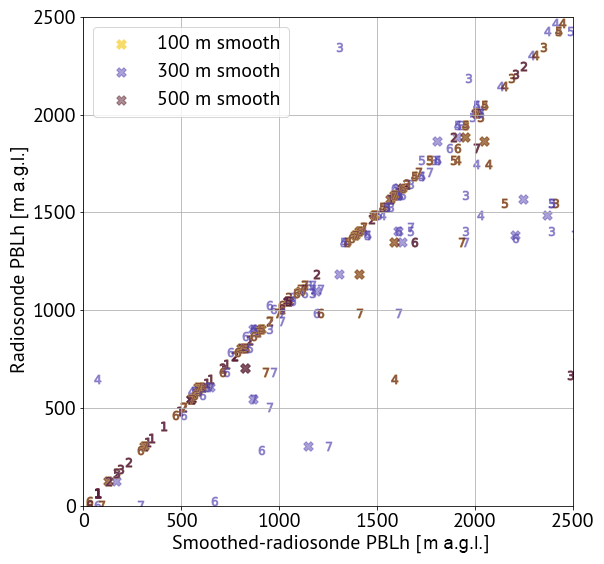
Figure 5 CHEESEHEAD sounding BL height estimates at the original vertical resolution compared with those from when 100, 300, and 500 m Savitzky–Golay smoothing is applied. The marker styles reference the BL height estimation technique, where an X marker indicates the median of all methods, and numbered markers reference the methods as they are listed in Table 2.

Holzworth (1964)Coniglio et al. (2013)Oke (1988)Stull (1988)Ao et al. (2008)Seidel et al. (2010)Bradley et al. (1993)Seidel et al. (2010)

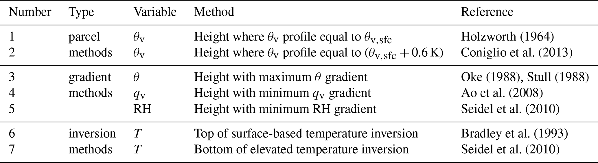
Table 2 Methods used to determine BL height from observed radiosonde data. Adapted from Seidel et al. (2010).

At SHV during PBLTops and whenever high-resolution data were otherwise unavailable, coarse-vertical-resolution, publicly available radiosonde observations were used instead. These radiosondes are provided with data recorded at mandatory and significant pressure levels. According to Schwartz and Govett (1992) these levels are determined for a variety of reasons, including but not limited to consistency between existing database conventions at the time of alignment. The resulting vertical resolution varies with height with an average spacing of 300 m; in the lower levels spacing is on the order of tens of meters, and in the upper levels spacing is on the order of several hundred meters. No smoothing was performed for the coarse soundings. Because exact launch times were not available for the coarse soundings, a launch time 1 h before the nominal time was assumed as per National Weather Service manual documentation of observation procedures (e.g., soundings denoted as 12:00 UTC were assigned a launch time of 11:00 UTC; National Weather Service, 2010).

Radiosondes were used to estimate BL height as a comparison for the fuzzy logic algorithm output. Numerous methods for estimating the BL height from radiosonde data have been proposed. BL height is a parameter which tends to be defined based on the application and data availability at hand. A one-size-fits-all definition has not been agreed upon in the meteorological community, its sub-communities, or tangential communities. Here, we utilize an ensemble of seven BL detection methods following Seidel et al. (2010). Our reasoning here is twofold. On one hand, it is useful to know if the fuzzy logic algorithm tends to match some methods more than others. This may mean the algorithm is more applicable in some settings or some important information is missing. On the other hand, and perhaps most interestingly, having an ensemble of estimates of BL height estimates provides a pseudo-measure of spread or uncertainty in the radiosonde estimation process itself. Large disparities between the given methods may suggest a more complex BL structure, increasing the level of difficulty for automated BL height detection.

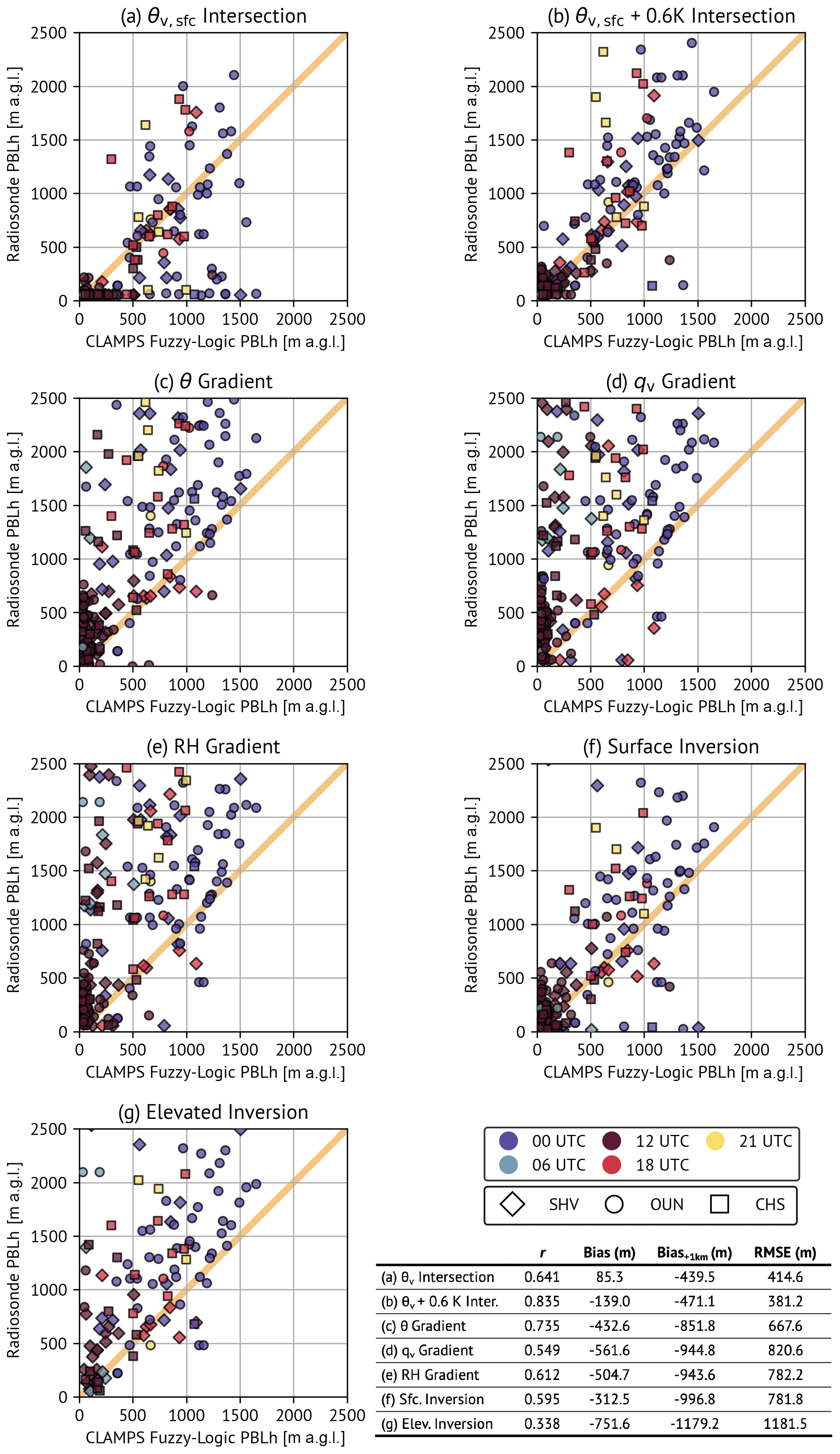
The first of the seven radiosonde-based methods described in Seidel et al. (2010), also known as the “parcel method”, finds the height at which the profile of virtual potential temperature θ_v becomes equal to the surface value. The second method extends this by adding 0.6 K to the surface θ_v value to prevent erroneously shallow BL estimates during the evening transition (Coniglio et al., 2013). The third, fourth, and fifth methods find the height of the maximum gradient of potential temperature θ, minimum gradient of water vapor mixing ratio q_v, and minimum gradient of relative humidity, respectively. The last two methods are inversion-based and find the top of any surface-based temperature inversion and the bottom of the lowest elevated temperature inversion layer, respectively. These methods are summarized in Table 2. To achieve an overall singular estimate of BL height from each sounding, the median of all available estimates is taken. To understand variability across the methods, the 25th and 75th percentile BL height estimate values are retained from the suite of methods. This approach was chosen as an outlier-resistant way to gather information about the variability among radiosonde-based BL height estimation methods.

Seidel et al. (2010) found that while coarse data can be sufficient to detect BL height, the use of high-resolution data can change the estimate in statistically significant ways. A comparison of the medians of radiosonde-derived BL heights in cases where high-resolution and coarse data were both available is shown in Fig. 6. This comparison initially appears to support the Seidel et al. (2010) findings. While many of the afternoon and early evening soundings are close to the one-to-one line, several of the morning soundings fall to the right and below the one-to-one line, suggesting the high-resolution-based estimates are lower than the coarse estimates. The “error” (more accurately, uncertainty) bars, which represent the spread (i.e., interquartile range) of BL heights detected by the seven methods, also appear to cover a wider range for the high-resolution soundings. However, if we further examine the comparison by looking at individual methods separately (Fig. 7), we find slightly different results than those in Seidel et al. (2010). Their results showed that methods computed from the surface up, such as the parcel- and inversion-based methods, were most sensitive to profile resolution, while Fig. 7 suggests that gradient-based methods are most sensitive in our dataset. Analyzing the methods separately highlights that using high-resolution sounding data tends to lead to lower median BL height, but the ranges and interquartile range values do not change much between coarse- and high-resolution datasets. To be certain, we conducted 10 000 bootstrap resampling analyses for each method to evaluate if the median and interquartile range values were significantly different between high- and coarse-resolution datasets. We found with 95 % confidence that there were no statistically significant differences. There is no indication from this analysis that using high-resolution data necessarily yields more accurate BL height values, and often users have access only to data that we have classified here as coarse-resolution (i.e., publicly available and accessible National Weather Service radiosonde datasets). Our intention with this analysis is to understand and consider possible implications of including different-resolution sounding datasets. Moving forward, we use high-resolution sounding data when they are available. If they are not available a coarse-resolution radiosonde profile is used instead.

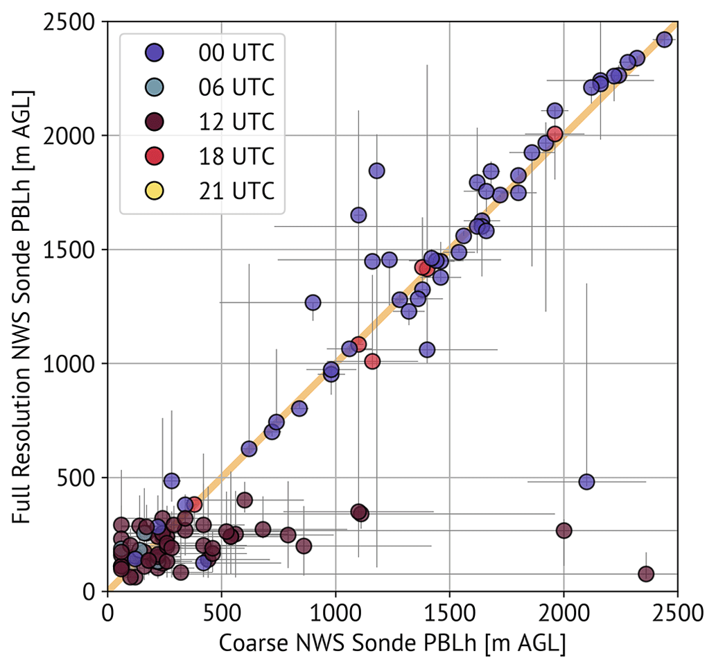
Figure 6 Comparison of BL heights derived from coarse, publicly available National Weather Service radiosonde data and BL heights derived via identical methods using the full-resolution radiosonde data not available on public archives. Points are color-coded based on nominal launch hour. Error bars (gray) represent the spread of BL heights derived from all methods described in the text as determined from the 25th and 75th percentiles.

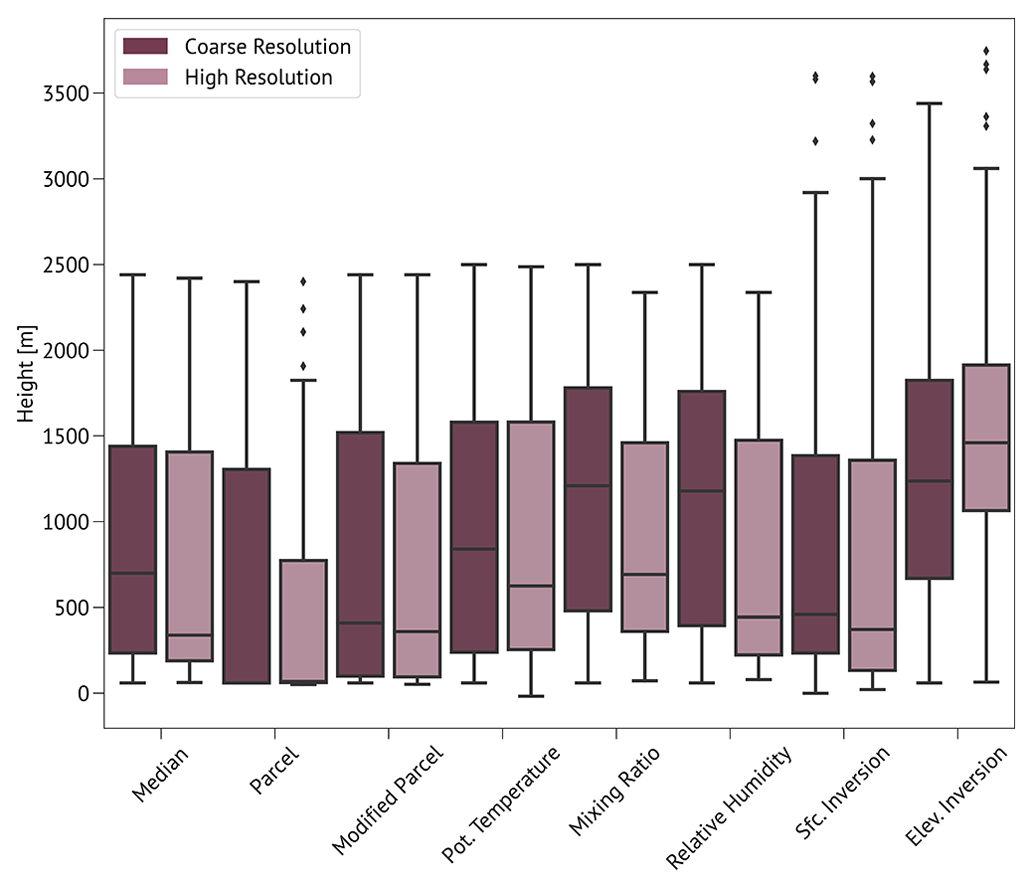
Figure 7 Box-and-whisker diagrams comparing radiosonde-based BL height estimates from coarse-resolution (dark shades) and high-resolution (light shades) datasets. Each box plot pair represents one radiosonde-based BL height estimation method (or, on the far left, the median of all methods). Only radiosonde profiles for which we had both coarse- and high-resolution data are included in this analysis. The cross-bars mark median values.

4 BL height estimate comparisons

Now we aim to understand how the fuzzy logic algorithm applied to CLAMPS data performs by comparing the resulting BL height estimates to BL height estimates from available radiosonde data. We use all the periods described in Sect. 3, always using high-resolution radiosonde profiles unless they are not available (e.g., some OUN launches during NWC/RIL and PBLTops; all SHV launches). All instances when a radiosonde value and fuzzy logic BL estimate are available at the same time (within ± 30 min) and place are shown together in Fig. 8. In Sect. 3.4, examination of the methods summarized in Seidel et al. (2010) highlights potential variability in BL height estimation based on radiosondes. In Fig. 9, the comparison from Fig. 8 is repeated for each method independently. Root mean square error (RMSE), correlation (r), and bias (computed for all values and computed only for instances when the BL height is 1 km or greater) are also shown. Upon visual inspection of the different methods, the comparisons between BL heights from radiosondes and BL height estimates from the fuzzy logic algorithm applied to CLAMPS observations take on different characteristics. For example, the modified parcel method (Fig. 9b) shows most BL height comparisons (not occurring at 12:00 UTC) collapsing toward the one-to-one line, indicating agreement between the approaches about the BL height. The correlation value when comparing fuzzy logic BL height to radiosonde-based BL height using the modified parcel method is the highest of all methods at 0.835. Conversely, using the elevated inversion method (Fig. 9g) in the comparison results in radiosonde-based BL height estimates nearly always being higher than those derived from the fuzzy logic algorithm applied to CLAMPS observations. In this instance, the correlation value is the lowest of all methods at 0.338. Selecting any one of these methods for deriving BL height from radiosondes could impact our understanding of the performance of the fuzzy logic algorithm applied to CLAMPS observations, since it would define the baseline against which the algorithm is compared. No one method is necessarily known to be more accurate than the others. In the absence of a well-justified or well-known definition of the top of the boundary layer that can be applied here, we proceed hereafter using the median of all methods (i.e., Fig. 8). We retain information about the range of BL height estimates produced by all the methods in the form of the interquartile range of BL height values. This approach allows us to have an outlier-resistant way to measure large variability across the radiosonde-based methods, which can suggest uncertainty in the radiosonde-based BL height estimate.

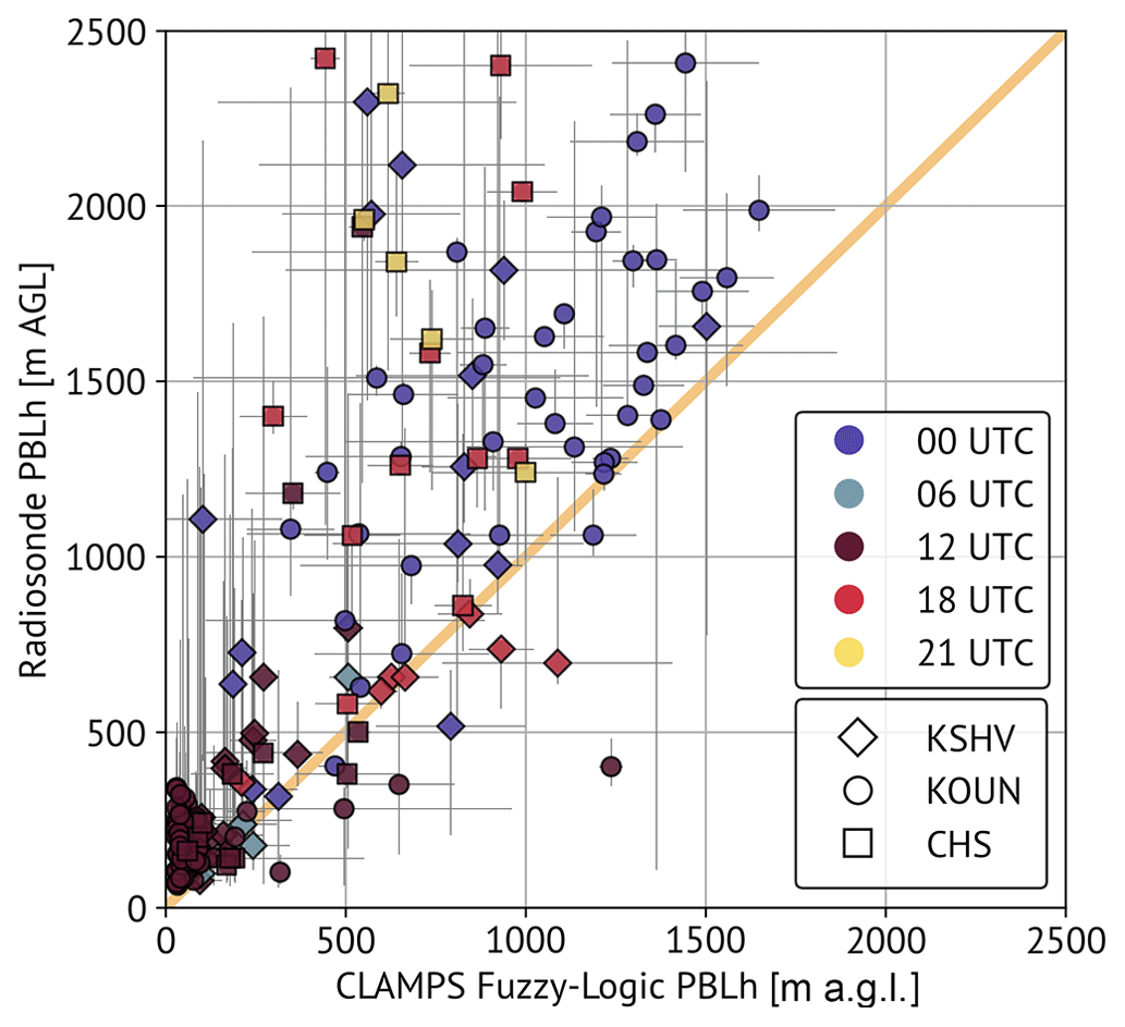
Figure 8 Comparison of CLAMPS-derived BL heights and median radiosonde-derived BL heights. Error bars (gray) indicate the range of BL heights detected within ± 30 min and the full range of BL heights from each method for the CLAMPS and radiosonde data, respectively.

Figure 9 As in Fig. 8, but for each of the seven individual BL height detection methods shown in Table 2. Root mean square error (RMSE), R², and bias (computed for all values and computed only for cases when the BL height is 1 km or greater) for each of the methods are shown in the table.

From the bulk comparison shown in Fig. 8, a few things become immediately apparent. The fuzzy logic method applied to CLAMPS observations is more likely to estimate a lower BL height than radiosondes. This is especially true in the afternoon hours, which correspond to 18:00 and 21:00 UTC for the areas where these observations were collected. No 21:00 UTC BL height comparisons (shown in yellow in Fig. 8) fall on or below the one-to-one line. The majority of 18:00 UTC and most 00:00 UTC BL height comparisons also trend above the one-to-one line, suggesting the fuzzy logic method applied to CLAMPS observations estimates a shallower BL. Earlier hours (06:00 and 12:00 UTC) do not demonstrate as much of a signal. While radiosondes generally cannot capture the temporal evolution of the BL in the same way remote sensors can, during the CHEESEHEAD campaign there is a window during which more frequent radiosonde releases are available. This period provides an opportunity to examine the fuzzy logic algorithm's behavior compared to radiosondes as a function of time in a different way. A series of fuzzy logic outputs following Fig. 3 for 4 d spanning 24–27 September 2023 is shown in Fig. 10. While there are differences on each day, these comparisons generally agree with what Fig. 8 shows: BL height estimates from soundings in earlier hours, in this case launches close to 12:00 and 14:00 UTC, agree more with the fuzzy logic estimates than afternoon sounding BL height estimates (i.e., launches from 18:00 and 21:00 UTC).

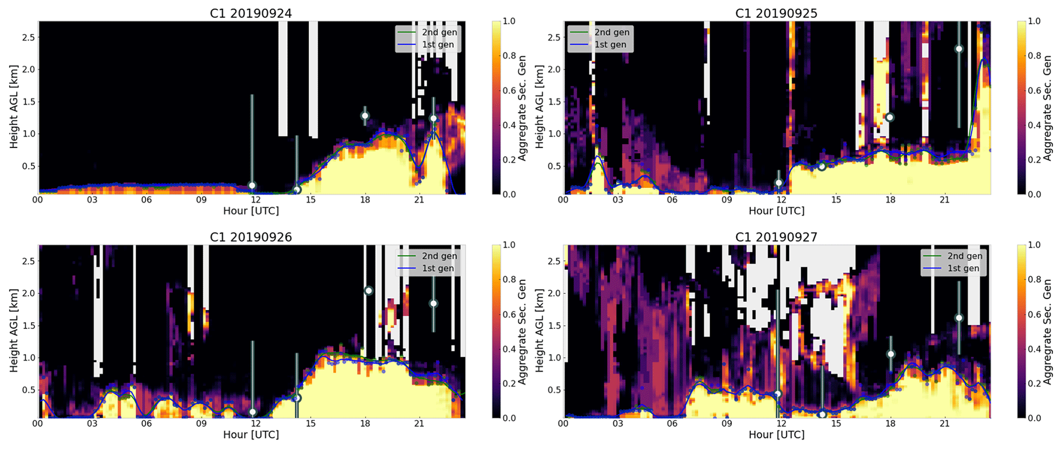
Figure 10 Fuzzy logic second-generation aggregates are shown based on CLAMPS1 observations from 4 d spanning 24–27 September 2019 during the CHEESEHEAD campaign. Soundings launched four times daily are overlaid on the aggregates, where the circle shows the median sounding BL height based on all sounding methods and the bars represent the interquartile range of BL heights from all sounding methods.

In Fig. 8, every available radiosonde–CLAMPS BL height estimate pair is compared without consideration of the atmospheric conditions at the time of the observation. In order to better understand the potential causes of discrepancies between the radiosonde and CLAMPS-based BL height estimates and ensure a robust comparison, each matched pair was manually interrogated for inclusion or exclusion in a similar approach as in Banghoff et al. (2018). In our case, criteria for exclusion were developed to describe instances in which discrepancies between CLAMPS and radiosonde BL heights may not necessarily reflect the intrinsic performance of the proposed algorithm. These criteria were as follows:

1. ambiguous cases where the BL height was unable to be confidently determined from the radiosonde data as multiple methods failed to identify BL height at all or identified levels that upon visual inspection were likely related to other structures (e.g., residual layer, clouds);

2. cases where CLAMPS observations were not able to be collected over a deep enough layer to capture the likely full depth of the BL (primarily DL observations due to a lack of scatterers);

3. cases where the BL top (e.g., entrainment layer or capping inversion) was deep and the radiosonde and CLAMPS methods identified different parts of this transition region; and

4. cases with complex and/or non-canonical BL structures (e.g., multiple inversions, low-level cloud layers).

To identify cases for exclusion, both authors independently evaluated each time-matched CLAMPS and radiosonde profile to determine whether one or more of these criteria were met without respect to how their BL height estimates compared, then discussed and reconciled any differences. These criteria were used to successively exclude data pairs and get a better sense of algorithm performance. As each criterion was applied successively, more pairs were removed from the comparison dataset as summarized in Table 3. Starting with 168 data pairs, 104 remained after all criteria were applied. The same set of statistics that were examined in the method comparison (r, bias, RMSE) is computed for each successively reduced dataset and shown in Table 3.

Table 3 Values computed for r, bias, and RMSE based on comparisons between the proposed fuzzy logic algorithm BL height estimates and radiosonde-based BL height estimates. The data source provides information about the campaign period and which CLAMPS platform collected observations which were then passed through the fuzzy logic algorithm.

Figure 11 shows comparisons of BL depth from CLAMPS and radiosondes for each sequential exclusion. Removing the cases where the BL height was ambiguous in the radiosonde data according to criterion (1) does not make much visual impact on the comparison (Fig. 11a). The pairs that are excluded follow no obvious pattern. They likely should not be expected to; cases where defining the BL height was ambiguous should lead to the CLAMPS-based method both over- and underestimating BL height compared to the radiosonde estimates without any physically defined trend. The same is not true for cases where the BL is too deep for the CLAMPS platforms to collect measurements over its full depth (criterion (2); Fig. 11b). These pairs are primarily found on the upper left side of the comparison diagram, meaning CLAMPS-based methods are underestimating these pairs. These cases occur in conditions where the CLAMPS observing systems simply cannot observe to a high-enough level above the surface. The algorithm's first step relies most heavily on DL-observed variables. If the BL is quite deep or for a variety of reasons (e.g., recent precipitation or other air mass characteristics) the scatterer load is low, the DL will not be able to reach levels above the surface where the BL height may reside. It is also true that the effective resolution of the thermodynamic profiles available from the platforms on board CLAMPS decays with increasing height above the surface. An exceptionally deep BL is simply difficult for the instruments on board to sample, and therefore the algorithm will also not be able to retrieve those BL height values well. With these pairs removed the comparison overall improves. Moving to a more quantitative comparison made available to us via statistics computed in Table 3, we see that the statistics generally improve when criterion (1) is applied. The r value modestly increases, while bias and RMSE both improve by 32.4 and 85.9 m, respectively. The percent bias also shows a decrease. When criterion (2) is additionally applied the improvements are more apparent. The r value increases further to 0.846. The bias and RMSE value improvements are the largest when this criterion is applied compared to any of the other criteria; the bias improves by 80.7 m and RMSE by 108.6 m. Percent bias also improves most drastically in this case. The pairs removed by criterion (2) are concentrated at greater BL height values, likely resulting in large improvements to statistics like bias. On the other hand, removals based on criterion (1) did not appear to follow any pattern, so improvements were distributed, resulting in more subtle impacts on the statistics.

Figure 11 As in Fig. 8, but with the exclusion of pairs to which criterion (1) applies (a) and successive exclusion of pairs to which criteria (1) and (2) apply (b), to which criteria (1)–(3) apply (c), and to which all criteria (1–4) apply (d).

Compared to Fig. 11b, Fig. 11c, which excludes criteria (1)–(3) including cases where the radiosonde and CLAMPS-based methods identified different parts of the BL top, shows fewer pairs in the area just above the one-to-one line. This suggests that when the two methods detect different parts of the BL top, the CLAMPS-based method is more likely to find a BL height closer to the surface. This makes sense as the fuzzy logic algorithm is a bottom-up algorithm that searches for the first point above the surface where the membership value crosses a threshold. As discussed previously, there is variability among chosen methods in how BL height is estimated from radiosonde data, and this is a scenario in which that variability can be important. Finally, Fig. 11d shows the comparison with all exclusion criteria applied (now additionally excluding complex BL structures). Compared to Fig. 11c, there are not obvious differences. The additional exclusions occur both above and below the one-to-one line. As for the ambiguous BL cases, this makes some sense as complex BL structures should not be expected to follow specific patterns, and we see the CLAMPS-based method both over- and underpredict BL height for these cases.

With all the exclusions applied, we can use the final set of remaining pairs shown in Fig. 11d as the so-called best cases for comparing the fuzzy logic algorithm to radiosonde-based BL heights. Differences in this comparison can be more directly attributed to characteristics of the proposed CLAMPS algorithm, or in other words these cases are those where the BL conditions are well-enough understood and represented by both sets of observation platforms for the comparison to be made. Many of the comparison pairs fall close to the one-to-one line, suggesting fairly good agreement between the fuzzy logic and radiosonde-based BL heights. When the pairs are not close to the one-one-line they tend to be above it, which indicates that in some cases the fuzzy logic algorithm applied to CLAMPS observations still leads to an underestimation of BL height compared to radiosonde-based BL heights. In this best-case comparison, we still see that the overnight and morning pairs (i.e., 06:00 and 12:00 UTC) are clustered together in the lower left side of Fig. 11b, which makes it difficult to examine patterns more closely. To better understand how the fuzzy logic algorithm compares to the radiosonde-based BL height estimates, we broke the best-case pairs with all exclusions applied into overnight–morning pairs (i.e., between 02:00 and 15:00 UTC) and afternoon–evening pairs (i.e., between 15:00 and 02:00 UTC the following day). Again, r, bias, percent bias, and RMSE are computed, but now for these subgrouped pairs based on time of day (values are reported in Table 3). The overnight–morning group (of the best case pairs) is a larger group than the afternoon–evening group. The r value is lower in the overnight–morning group, while both bias and RMSE appear to be improved compared to the afternoon–evening group. This is misleading, however, as a bias of 100 m in the overnight or morning hours is much more impactful than during the afternoon hours when the BL is fully developed and much deeper. Percent bias may be more informative, since it is expressed in terms of a percentage of the absolute value of the reference value (in this case, the radiosonde BL height estimates are the reference values). The morning percent bias (−42.5 %) is roughly twice the afternoon bias (−20.8 %), reflecting the difference in relative scale between the morning and afternoon BL. In any case, these subgroups show different results than the full best-case pairs group, suggesting that the time of day has an impact on the comparison between the radiosonde-based estimates and the fuzzy logic algorithm. With more frequent and regularly available radiosondes, this analysis could lead to a deeper understanding of the impact that time of day has on the performance of the fuzzy logic algorithm itself.

5 Summary and outlook

In this work, we present a fuzzy logic approach for estimating BL height that incorporates kinematic and thermodynamic observation data streams into a multi-instrument value-added product. This algorithm expands from the work of Bonin et al. (2018), specifically by including thermodynamic profiles. The fuzzy logic algorithm follows a two-step process to produce BL height estimates using various input observations from the kinematic and thermodynamic observing platforms on board the CLAMPS facilities. Output is produced every 10 min along with standard deviations from an hour-wide centered sliding window. While this algorithm was developed for use with the CLAMPS platforms (i.e., a Doppler lidar, infrared spectrometer, and microwave radiometer), it could be applied to or adapted for similarly instrumented facilities such as but not limited to the Department of Energy's Atmospheric Radiation Measurement profiling facilities.

To characterize and understand how the presented algorithm performs, it is compared with radiosonde data collected from three periods: the CHEESEHEAD project in Wisconsin during the fall of 2019, the NWC/RIL deployment in Oklahoma during summer 2020, and the PBLTops project in Oklahoma and Louisiana during summer and fall 2020. To make sure these comparisons are well suited, various impacts of radiosonde data resolution are examined (i.e., impacts of vertical spacing on gradient calculations and high-resolution versus coarse-resolution comparisons). This analysis does not aim to present the most correct method for computing BL height from radiosondes, but it shows the differences between methods and possible variability that can be introduced when including sounding datasets with different resolutions.

Comparisons are conducted in two ways, the first of which is a bulk comparison of all instances when a radiosonde-based estimate and fuzzy logic estimate of BL height are available at the same time (within ± 30 min) and place. Through this analysis we show that the fuzzy logic algorithm often results in lower BL height estimates than radiosonde-based methods (especially in the afternoon hours). When examining this comparison more closely, we find sensitivity to the exact BL height estimation method applied to radiosonde data as expected. As was the case for the analysis of radiosonde data resolution, we do not intend to offer any one radiosonde-based BL height estimation method as preferred. In our application, using the median provides a basis for comparison, and the 25th and 75th percentile BL height estimate values are retained from the suite of methods as an outlier-resistant measure of variability. However, this sensitivity to BL height estimation method (and potentially to the resolution of radiosonde data, as noted above) presents a nontrivial complicating factor for any use case. It is also a factor worth considering for comparing findings across past studies.

Comparisons are again conducted, but this time consideration is given to the atmospheric conditions at the time of the matched radiosonde–CLAMPS profile observation with the intention of understanding and eliminating extrinsic causes for discrepancies between the radiosonde-based BL estimates and results from the fuzzy logic algorithm. Each radiosonde–CLAMPS observation pair was manually interrogated and either included or excluded. Criteria for exclusion can be summarized as follows: (1) ambiguous, (2) BL too deep for CLAMPS observation capability, (3) deep BL top (e.g., deep capping inversion or entrainment layer), and (4) complex and/or non-canonical. The exclusions are applied successively, eventually leading to a final subset of best cases in which the BL conditions are well-enough understood and represented by both sets of observation platforms for a robust comparison to be made between the fuzzy logic algorithm and radiosonde-based BL height estimates. This comparison suggests fairly strong agreement between the techniques, but still with a maintained pattern of the fuzzy logic algorithm applied to CLAMPS observations underestimating BL height compared to the median of radiosonde-based methods. Given the instrumentation types included in the algorithm development and evaluation (Doppler lidar, infrared spectrometer, microwave radiometer), we speculate that even in the best-case comparisons, remote-sensing-based observations are simply more inclined to detect the lowest possible indication of BL height (especially in cases where the BL top itself may be a layer with appreciable depth). These types of instruments are also more likely to lose measurement capability and resolution with distance from the surface. These reasons could combine to result in systematically lower estimates of BL height than those provided by in situ platforms like radiosondes.

Unlike some similar algorithms, this approach has the capability to utilize thermodynamic observation information and kinematic observation information to provide BL height estimates throughout the diurnal cycle. Specific analysis is focused on the early morning and late overnight periods. While some statistics included suggest perhaps even minor improvement compared to the daytime group, this may be a misleading result. For example, a bias of 100 m means something different when the BL height is 𝒪(100 m), which is common in the overnight and morning hours, compared to 𝒪(1000 m) BL height values in a fully developed daytime and afternoon BL. More data are needed in this comparison to understand the role time of day plays in how the fuzzy logic algorithm behaves. More data could provide the opportunity to build time-dependent samples or to develop temporal normalization approaches to control for this important sensitivity.

There are various techniques for observing the lower atmosphere, which individually offer an incomplete picture of the processes that characterize the BL. Methods of BL characterization, including BL height, can be subjective. These sources of ambiguity in understanding the BL can be addressed through synergistic combination of observation techniques. Kotthaus et al. (2023) describe the potential for instrument synergy to advance methodologies and products and to provide value in process studies and applications. Specifically, they identify the potential of using multiple observing platforms to extend detection capabilities beyond those of individual platforms, suggested assessment of uncertainty among techniques, and employment of advanced retrieval techniques (e.g., fuzzy logic). The fuzzy logic algorithm presented in this work combines Doppler lidar, infrared spectrometer, and microwave radiometer observations to produce relatively high-resolution BL height estimates with an assessment of uncertainty or variability. In the last 5 years, there has been a flurry of renewed interest in BL height retrieval capabilities of the NWS NEXRAD network (e.g., Banghoff et al., 2018; Comer et al., 2023; Della Porta, 2024; Loeffler and Davies, 2024; Stensrud et al., 2024; Stouffer et al., 2024). Algorithms such as the one described in this study, which produce an independent reference dataset of the full diurnal evolution of PBL height to compare against, will provide important context for validating these novel BL height monitoring methods. To this end, a follow-on study to the present work explores using BL height estimates from this fuzzy logic algorithm applied to CLAMPS observations to gain insight into radar-based boundary-layer height estimates in ways that temporally limited radiosonde profiles cannot. While in its first testing iteration, the fuzzy logic algorithm has already been deployed in research comparing BL height methods across research-grade tools during the CHEESEHEAD project (Duncan et al., 2022). It is currently in use for ongoing research related to several recent field programs and deployments on which CLAMPS has been deployed such as the TRacking Aerosol Convection interactions ExpeRiment (TRACER) and the American WAKE experimeNt (AWAKEN). The algorithm has been de facto integrated into the suite of tools frequent CLAMPS users implement in their own research, and there are plans to explore implementing it as part of the data system workflow as a value-added product for standard CLAMPS operations. To facilitate further applications and use cases the fuzzy logic BL height detection algorithm implementation has been made available on a dedicated GitHub repository, BLISS-FL (Boundary-Layer height Inferred through multi Sensor Synergy-Fuzzy Logic; see the “Code and data availability” statement for access information). In the spirit of open science, making the algorithm available encourages collaboration, adaptation, and extension for ongoing algorithm refinement and enhancement. We invite readers to engage with the algorithm, contribute to its development, and apply it to diverse problems and datasets.