Uncertainties in temperature statistics and fluxes determined by sonic anemometers due to wind-induced vibrations of mounting arms

Accurate air temperature measurements are essential in eddy covariance systems, not only for determining sensible heat flux but also for applying density effect corrections (DECs) to water vapor and CO₂ fluxes. However, the influence of wind-induced vibrations of mounting structures on temperature fluctuations remains a subject of investigation. This study examines 30 min average temperature variances and fluxes using eddy covariance systems, combining Campbell Scientific sonic anemometers with closely co-located fine-wire thermocouples alongside LI-COR CO₂–H₂O gas analyzers at multiple heights above a sagebrush ecosystem. The variances of sonic temperature after humidity corrections (T_s) and sensible heat fluxes derived from T_s are underestimated (e.g., by approximately 5 % for temperature variances and 4 % for sensible heat fluxes at 40.2 m, respectively) as compared with those measured by a fine-wire thermocouple (T_c). Spectral analysis illustrates that these underestimated variances and fluxes are caused by the lower energy levels in the T_s spectra than the T_c spectra in the low-frequency range (natural frequency < 0.02 Hz). These underestimated T_s spectra in the low-frequency range become more pronounced with increasing wind speeds, especially when wind speed exceeds 10 m s⁻¹. Moreover, the underestimated temperature variances and fluxes cause overestimated water vapor and CO₂ fluxes through DEC. Our analysis suggests that these underestimations when using T_s are likely due to wind-induced vibrations affecting the tower and mounting arms, altering the time of flight of ultrasonic signals along three sonic measurement paths. This study underscores the importance of further investigations to develop corrections for these errors.

1 Introduction

The eddy covariance (EC) technique has been widely used to measure turbulent fluxes of heat, water vapor, CO₂, and other scalars between terrestrial ecosystems and the atmosphere (Chu et al., 2021; Lee et al., 2014; Missik et al., 2021; Tang et al., 2019; Wang et al., 2010). It is instrumental in studying micrometeorological processes in the atmospheric surface layer (Eder et al., 2013; Gao et al., 2018; Guo et al., 2009; Li et al., 2018; Zhang et al., 2010). Despite considerable advancement in the EC technique (Burns et al., 2012; Frank et al., 2013; Fratini et al., 2012; Horst et al., 2015; Liu et al., 2001; Mauder et al., 2007; Mauder and Zeeman, 2018; Wilczak et al., 2001), uncertainties in EC fluxes remain a great concern (Loescher et al., 2005; Massman and Clement, 2006; Peña et al., 2019), including the notable issue of the surface energy balance closure (Mauder et al., 2020). Thus, improving the accuracy of EC flux measurements and identifying the potential sources of uncertainties in these fluxes are critically important.

In most EC applications, sonic-derived air temperature is usually employed after corrections for determining sensible heat fluxes (H) (Liu et al., 2001; Schotanus et al., 1983). However, erroneous H values determined by sonic anemometers have been reported, especially under high wind conditions (e.g., Burns et al., 2012; Smedman et al., 2007). For instance, Smedman et al. (2007) utilizing two co-located Gill sonic anemometers (models R2 and R3) observed that sonic-determined H exhibited larger magnitudes than H measured with an alternative temperature sensor. They also noted that for wind speed exceeding 10 m s⁻¹, a correction highly dependent on wind speed is essential for sonic-determined H (Smedman et al., 2007). Burns et al. (2012), employing a Campbell Scientific sonic anemometer (model CSAT3) and a co-located type-E thermocouple (wire diameter of 0.254 mm), reported substantial errors for H determined from the CSAT3 sonic anemometer with a firmware of version 4.0 for wind speed above 8 m s⁻¹. Such large errors in H result from inaccurate sonic-derived temperature due to an underestimation of the speed of sound, though errors caused by sonic anemometer transducer shadowing can also cause errors in H (Frank et al., 2013; Horst et al., 2015). Wind-induced vibrations in the tower and mounting arms, particularly under windy conditions, were speculated to be potential contributors, causing spikes in the signals of sonic temperature (Burns et al., 2012). However, the precise impact of vibration-induced errors in sonic-derived temperature on temperature variances and sensible heat fluxes, especially for tall towers under strong wind conditions, has remained unexplored.

Accurate air temperature measurements are not only important for determining H but also crucial for estimating other scalar fluxes (e.g., water vapor and CO₂) through density effect corrections (DECs hereafter; Detto and Katul, 2007; Gao et al., 2020; Lee and Massman, 2011; Sahlée et al., 2008; Webb et al., 1980). The measured high-frequency time series of densities of water vapor, CO₂, and other scalars are subject to the effects of density fluctuations of dry air and other components in the atmosphere, as well as the fluctuations of air pressure (Lee and Massman, 2011; Webb et al., 1980). Correcting for these effects involves applying corrections to either the calculated raw fluxes or the high-frequency time series of the scalar density fluctuations (Webb et al., 1980; Detto and Katul, 2007; Gao et al., 2020; Sahlée et al., 2008). Any errors or uncertainties in sonic-derived temperature are anticipated to propagate and, in some certain cases, be amplified by the correction algorithms applied to the scalar fluxes, leading to heightened uncertainties in these fluxes (Liu et al., 2006).

The objective of this study is to scrutinize the uncertainties in temperature statistics and fluxes determined by sonic anemometers, with particular attention to the potential influence of vibrations of the tower and mounting arms under high wind speeds. The data employed were collected from three levels of Campbell Scientific sonic anemometers (model CSAT3B) alongside co-located fine-wire thermocouples and open-path infrared gas analyzers. By comparing the sensible heat fluxes calculated using air temperature from the sonic anemometers and the thermocouples, we assess vibration-induced errors in sensible heat fluxes at the three heights. The findings reveal that the sonic anemometers underestimate the temperature variances and fluxes compared to the thermocouples. Furthermore, we investigate the propagation of these vibration-induced errors to water vapor and CO₂ fluxes through the density effect corrections.

2 Materials and methods

2.1 Experiment and data

The experiment was conducted at the National Oceanic and Atmospheric Administration (NOAA) Grid 3 area (station ID: GRI) situated on the western edge of the Snake River Plain in southeastern Idaho, USA (43.59° N, 112.94° W; 1500 m above mean sea level; Fig. 1). The closest mountains are located approximately 13 km northwest from GRI. Based on the data from multiple automated meteorological observation stations in the area, southwesterly and northeasterly winds prevail during the day and night, respectively (Finn et al., 2016). Under these prevailing winds, GRI has a relatively flat and uniform upwind fetch (Finn et al., 2018; Lan et al., 2018). The vegetation primarily comprises shrubs and grasses, each with a roughness length and displacement height of a few centimeters (Finn et al., 2016).

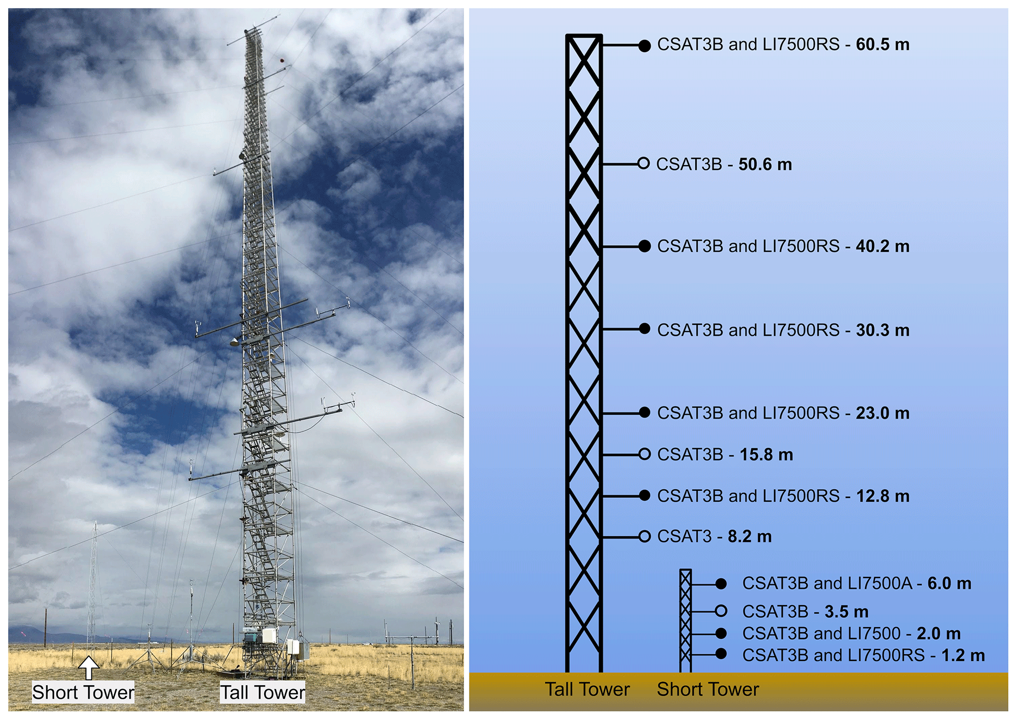
Figure 1 Photo of the 62 and 10 m towers at the Idaho National Laboratory (INL) site in southeastern Idaho and the instrumentational configuration of the field study.

The experiment utilized a 62 m tower and a 10 m aluminum tower (UT30, Campbell Scientific, Inc.) at the Grid 3 area to mount the sensors (Fig. 1). The 62 m tower was guyed at eight levels, and the 10 m tower was guyed at one level. Retractable square booms measuring 3.6 m (12 ft) were horizontally braced to the 62 m tower to attach the sensors. The CSAT3s and IRGAs were mounted on 1 ft pipes, which were securely attached to the end of each boom. As a result, the CSAT3s and IRGAs were positioned at least 2.0 m away from the tower structure. On the 10 m tower, 1.8 m (6 ft) poles were utilized to mount the CSAT3s and IRGAs, positioning the sensors approximately 1.5 m away from the tower's frame structures.

Throughout the experiment, multiple levels of EC systems were deployed (Fig. 1). These EC systems included two models of 3D sonic anemometers from the same manufacturers (model CSAT3B and CSAT3, Campbell Scientific, Inc.) and three models of infrared gas analyzers from the same manufacturers (IRGA; model LI7500RS, LI7500A, and LI7500, LICOR, Inc.). CSAT3s measured the three-dimensional wind velocity components (u, v, and w) and the sonic air temperature (T_{s_m}), while IRGAs measured the densities of water vapor (ρ_v) and CO₂ (ρ_c). Co-located with CSAT3s and IRGAs, Type-E fine-wire thermocouples (model FW3, Campbell Scientific, Inc.) were used to measure air temperature (T_c) at six heights of 2.0, 8.2, 12.8, 15.8, 23.0, and 40.2 m. The FW3 thermocouple is composed of a chromel wire and a constantan wire with a diameter of 0.0762 mm. The FW3 determines T_c by measuring the voltage potential differences created at the junction of the two wires due to the temperature difference, whereas T_{s_m} is determined based on the relationship between sonic virtual temperature and the speed of sound (Liu et al., 2001). This distinction in temperature measurement principles between CSAT3s and FW3 implies that the measured T_{s_m} and T_c are independent of each other. Furthermore, T_c is expected to remain unaffected by vibrations of the tower and mounting arms. In this study, we also recorded the inclination of the CSAT3B (e.g., pitch and roll angle measurements) given by an integrated inclinometer in the CSAT3B. Pitch angle is defined as the angle between the gravitationally horizontal plane and the CSAT3B x axis, and roll angle is defined as the angle between the gravitationally horizontal plane and the CSAT3B y axis. The sonic roll and pitch angles were stored as 30 min averages.

Three dataloggers (model CR1000X, Campbell Scientific, Inc.) were employed to sample the high-frequency instruments (i.e., sonic anemometer, fine-wire thermocouple, and gas analyzer) at 10 Hz. Each datalogger was equipped with a GPS receiver (model GPS16X-HVS, Garmin International, Inc.) to synchronize the datalogger clocks. Additionally, a variety of meteorological measurements were conducted at GRI, including net radiation, air temperature, relative humidity, soil moisture, soil temperature, and soil heat fluxes. In this study, we examined the data collected at three different heights (40.2, 23.0, and 12.8 m) from 25 April to 31 July 2021, considering structural differences between the tall tower and short tower setups as well as potential influences from the roughness sublayer on measurement at lower levels.

2.2 Post-field data processing

The data processing mainly entailed despiking, double rotation for the wind components (Wilczak et al., 2001), sonic temperature conversion (Liu et al., 2001; Schotanus et al., 1983), and application of DEC to the raw fluxes of latent heat and CO₂ (Webb et al., 1980). However, corrections for the effects of humidity and density fluctuations in this study are applied to the turbulent fluctuations of sonic temperature, ρ_v, and ρ_c, respectively (Detto and Katul, 2007; Gao et al., 2020; Sahlée et al., 2008; Schotanus et al., 1983; Webb et al., 1980). For each 30 min interval, the corrected turbulent fluctuations of sonic temperature ($T_{\mathrm{s}}^{\prime }$), ${\mathit{\rho }}_{\mathrm{v}}^{\prime }$, and ${\mathit{\rho }}_{\mathrm{c}}^{\prime }$ are determined by

$$\begin{array}{}\text{(1)}& {\displaystyle }{T}_{\mathrm{s}}^{\prime }\left(t\right)=T_{\mathrm{s}\mathit{\_}\mathrm{m}}^{\prime }\left(t\right)-\mathrm{0.51}{\displaystyle \frac{{\mathit{\rho }}_{\mathrm{v}}^{\prime }\left(t\right)}{{\stackrel{\mathrm{‾}}{\mathit{\rho }}}_{\mathrm{a}}}}\stackrel{\mathrm{‾}}{T}\end{array}$$

$$\begin{array}{}\text{(2)}& {\displaystyle }& {\displaystyle }{\mathit{\rho }}_{\mathrm{v}}^{\prime }\left(t\right)=(\mathrm{1}+\mathit{\mu }\mathit{\sigma }){\mathit{\rho }}_{\mathrm{v}\mathit{\_}\mathrm{m}}^{\prime }\left(t\right)+(\mathrm{1}+\mathit{\mu }\mathit{\sigma }){\displaystyle \frac{{\stackrel{\mathrm{‾}}{\mathit{\rho }}}_{\mathrm{v}}}{\stackrel{\mathrm{‾}}{T}}}{T}_{\mathrm{s}}^{\prime }\left(t\right)\text{(3)}& {\displaystyle }& {\displaystyle }{\mathit{\rho }}_{\mathrm{c}}^{\prime }\left(t\right)={\mathit{\rho }}_{\mathrm{c}\mathit{\_}\mathrm{m}}^{\prime }\left(t\right)+{\stackrel{\mathrm{‾}}{\mathit{\rho }}}_{\mathrm{c}}(\mathrm{1}+\mathit{\mu }\mathit{\sigma }){\displaystyle \frac{T_{\mathrm{s}}^{\prime }\left(t\right)}{\stackrel{\mathrm{‾}}{T}}}+\mathit{\mu }{\displaystyle \frac{{\stackrel{\mathrm{‾}}{\mathit{\rho }}}_{\mathrm{c}}}{{\stackrel{\mathrm{‾}}{\mathit{\rho }}}_{\mathrm{a}}}}{\mathit{\rho }}_{\mathrm{v}}^{\prime }\left(t\right),\end{array}$$

where T_{s_m}, ρ_{v_m}, and ρ_{c_m} represent measured sonic temperature, water vapor, and CO₂ densities, respectively; $\stackrel{\mathrm{‾}}{T}$, ${\stackrel{\mathrm{‾}}{\mathit{\rho }}}_{\mathrm{a}}$, ${\stackrel{\mathrm{‾}}{\mathit{\rho }}}_{\mathrm{v}}$, and ${\stackrel{\mathrm{‾}}{\mathit{\rho }}}_{\mathrm{c}}$ are averages of air temperature, air density, water vapor, and CO₂ densities, respectively; $\mathit{\mu }=m_{\mathrm{d}}/m_{\mathrm{v}}$ (m_d and m_v are the molecular mass of dry air and water vapor, respectively); and $\mathit{\sigma }={\stackrel{\mathrm{‾}}{\mathit{\rho }}}_{\mathrm{v}}/{\stackrel{\mathrm{‾}}{\mathit{\rho }}}_{\mathrm{d}}$ (${\stackrel{\mathrm{‾}}{\mathit{\rho }}}_{\mathrm{d}}$ is the density of dry air). The prime symbol denotes the turbulent fluctuations relative to the 30 min block average. As shown in the equations above, there is interdependence between $T_{\mathrm{s}}^{\prime }$ and ${\mathit{\rho }}_{\mathrm{v}}^{\prime }$, and thus $T_{\mathrm{s}}^{\prime }$ and ${\mathit{\rho }}_{\mathrm{v}}^{\prime }$ must be determined iteratively. In this study, the corrections are iterated twice. Note that in semiarid sites like ours, the adjustments to $T_{\mathrm{s}}^{\prime }$ due to fluctuations in specific humidity ($\frac{{\mathit{\rho }}_{\mathrm{v}}^{\prime }\left(t\right)}{{\stackrel{\mathrm{‾}}{\mathit{\rho }}}_{\mathrm{a}}}$) are typically negligible (not shown here) as compared to the adjustment to ${\mathit{\rho }}_{\mathrm{v}}^{\prime }$ due to fluctuations in $T_{\mathrm{s}}^{\prime }$ (as demonstrated in Sect. 3.5). The corrected time series of fluctuations facilitate the investigation of coherent structures and scalar similarity between temperature and other scalars (Detto and Katul, 2007; Sahlée et al., 2008). Here and throughout, T_s refers to the air temperature measured by sonic anemometers after humidity corrections, T_{s_m} the sonic temperature directly measured before corrections, and T_c the air temperature measured by fine-wire thermocouples (FW3).

2.3 Ensemble empirical mode decomposition (EEMD)

Ensemble empirical mode decomposition (EEMD) (Huang et al., 1998; Huang and Wu, 2008) is applied to decompose the 30 min turbulence time series into three subsequences, corresponding to the high-, middle-, and low- frequency ranges, respectively. EEMD is a favored method in analyzing non-linear and non-stationary turbulence data (Gao et al., 2018; Hong et al., 2010; Liu et al., 2021; Huang et al., 1998; Huang and Wu, 2008). Through the sifting process in EEMD, a 30 min time series is decomposed into 13 oscillatory components C_j(t) ($j=\mathrm{1},\mathrm{2},\mathrm{\dots },\mathrm{13}$) and an overall residual r₁₃(t). Each oscillatory component generally exhibits one characteristic frequency (Hong et al., 2010; Gao et al., 2018), while the overall residual either is monotonic or contains only one extremum, from which no more oscillatory components can be further decomposed. Hence,

$$\begin{array}{}\text{(4)}& x\left(t\right)=r_{\mathrm{13}}\left(t\right)+{\sum }_{j=\mathrm{1}}^{\mathrm{13}}{C}_j\left(t\right).\end{array}$$

As detailed in Sect. 3.2, after comparing the power spectra of T_s and T_c, two frequency boundaries, 0.02 and 0.2 Hz, are identified. The oscillatory components are then categorized into three frequency ranges (I, II, and III, respectively). The oscillatory components with mean frequencies falling within the corresponding ranges are added together to generate the three subsequences. Specifically, oscillatory components with mean frequencies smaller than 0.02 Hz are summed and labeled as regime I (i.e., $x_{\mathrm{I}}^{\prime }=\sum _{j=\mathrm{10}}^{\mathrm{13}}{C}_{j,x}+r_{\mathrm{13}}$, where x=w, T_s, and T_c), between 0.02 and 0.2 Hz as regime II (i.e., $x_{\text{II}}^{\prime }=\sum _{j=\mathrm{6}}^{\mathrm{9}}{C}_{j,x}$), and larger than 0.2 Hz as regime III (i.e., $x_{\text{III}}^{\prime }=\sum _{j=\mathrm{1}}^{\mathrm{5}}{C}_{j,x}$).

3 Results and discussion

3.1 Comparison of the CSAT3B- and FW3-derived temperature variances and fluxes

Figure 2 illustrates the comparisons between the variances and fluxes obtained using T_s and T_c at different heights. Here, we use ${\mathit{\sigma }}_{T_{\mathrm{c}}}^{\mathrm{2}}$ and $\stackrel{\mathrm{‾}}{w^{\prime }{T}_{\mathrm{c}}^{\prime }}$ as reference values since T_c is less sensitive to the effects of humidity and wind speeds than T_s (Burns et al., 2012; Smedman et al., 2007). Generally, the variances of T_s (${\mathit{\sigma }}_{T_{\mathrm{s}}}^{\mathrm{2}}$) are smaller than variances of T_c (${\mathit{\sigma }}_{T_{\mathrm{c}}}^{\mathrm{2}}$), typically by 2 %–5 % (Fig. 2a–c). These lower variances result in a lower sensible heat flux ($\stackrel{\mathrm{‾}}{w^{\prime }{T}_{\mathrm{s}}^{\prime }}$). Specifically, at 23.0 and 40.2 m, $\stackrel{\mathrm{‾}}{w^{\prime }{T}_{\mathrm{s}}^{\prime }}$ is underestimated by approximately 2 % and 4 %, respectively, as compared to the sensible heat fluxes derived from the FW3 (i.e., $\stackrel{\mathrm{‾}}{w^{\prime }{T}_{\mathrm{c}}^{\prime }}$) (Fig. 2d and e). However, at 12.8 m, $\stackrel{\mathrm{‾}}{w^{\prime }{T}_{\mathrm{s}}^{\prime }}$ and $\stackrel{\mathrm{‾}}{w^{\prime }{T}_{\mathrm{c}}^{\prime }}$ are quite comparable (Fig. 2f). These results confirm that errors in H were not entirely due to errors in the vertical velocity (Frank et al., 2013; Horst et al., 2015). Further examination of Fig. 2 reveals that the differences between ${\mathit{\sigma }}_{T_{\mathrm{s}}}^{\mathrm{2}}$ and ${\mathit{\sigma }}_{T_{\mathrm{c}}}^{\mathrm{2}}$, as well as between $\stackrel{\mathrm{‾}}{w^{\prime }{T}_{\mathrm{s}}^{\prime }}$ and $\stackrel{\mathrm{‾}}{w^{\prime }{T}_{\mathrm{c}}^{\prime }}$, increase with increasing measurement heights. Additionally, our tests indicate that the influence of solar heating on measurements of FW3 is negligible, primarily due to the fine-wire diameter of 0.0762 mm (Text S1 and Fig. S1 in the Supplement).

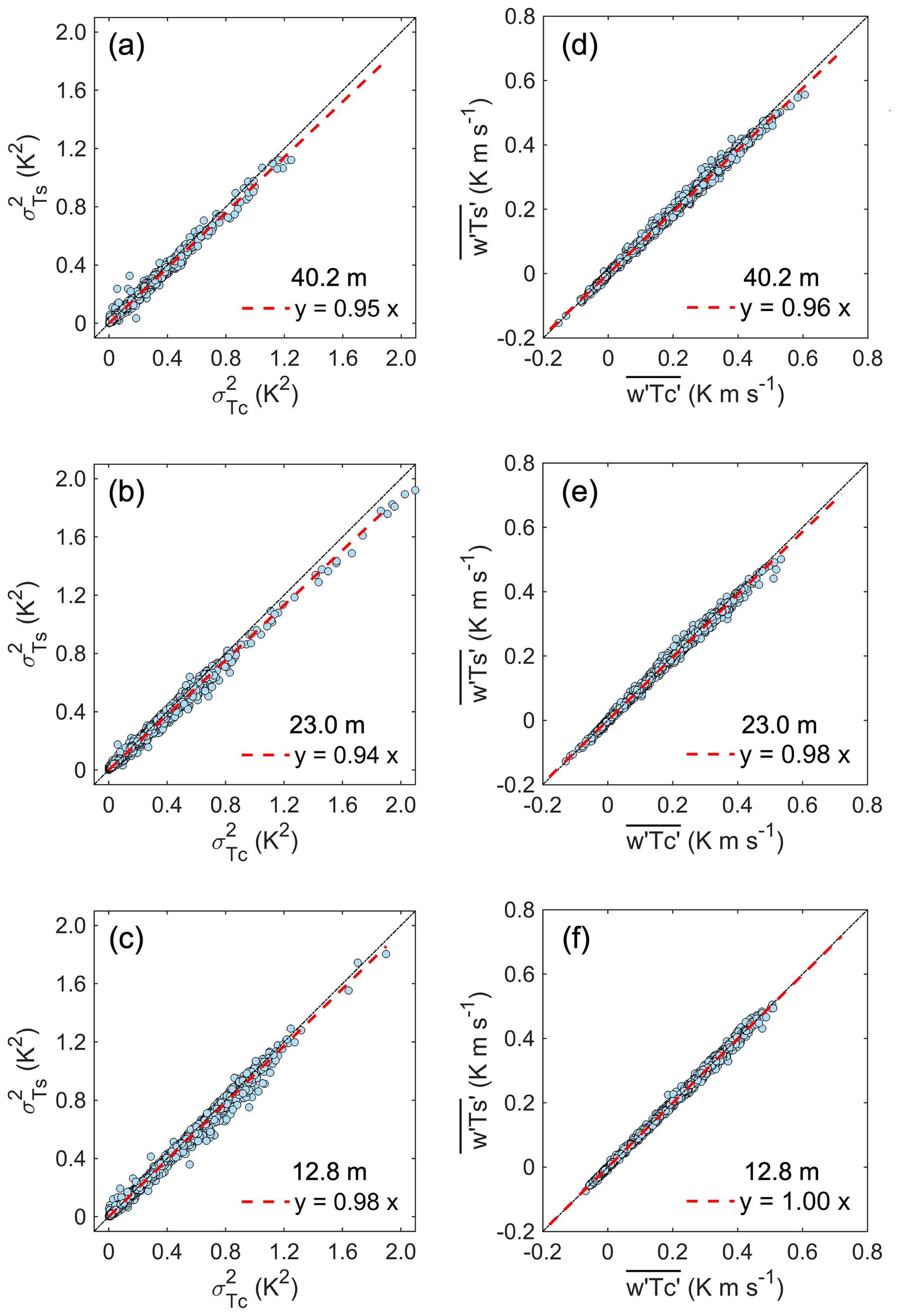
Figure 2 Comparison of temperature variances and sensible heat fluxes computed using T_s and T_c at the heights of 40.2, 23.0, and 12.8 m, respectively.

What mechanisms could have caused the observed differences? Previous studies found that CSAT3 sonic anemometers with a previous version of firmware could cause errors in T_s (Burns et al., 2012). However, this should not be the case for our study because the CSAT3B modes were used at these heights, and they have an improved design compared to the original CSAT3. Our results suggest that the differences are dependent on the measurement heights. As the measurement heights increase, the dominant length scale of coherent structures is also enlarged (Zhang et al., 2011). Therefore, we conjecture that the processes that lead to such differences are most likely scale-dependent, motivating us to examine the spectra and cospectra in the next subsection.

3.2 Spectral comparisons

To gain further insight into the differences between ${\mathit{\sigma }}_{T_{\mathrm{s}}}^{\mathrm{2}}$ and ${\mathit{\sigma }}_{T_{\mathrm{c}}}^{\mathrm{2}}$ as well as the associated fluxes (i.e., $\stackrel{\mathrm{‾}}{w^{\prime }{T}_{\mathrm{s}}^{\prime }}$ and $\stackrel{\mathrm{‾}}{w^{\prime }{T}_{\mathrm{c}}^{\prime }}$), the spectra of u, w, T_s, and T_c and the w–T_s and w–T_c cospectra at different heights are examined. Figure 3a–c show the mean normalized Fourier power spectra of u, w, T_s, and T_c as a function of natural frequency (f). Note that the power spectra were computed every half hour using the fast Fourier transform and normalized by the corresponding variances before averaging. It is also interesting to note that the u, w, and T_s spectra deviate from the well-known $-\mathrm{5}/\mathrm{3}$ power law in the high-frequency range of f > 0.2 Hz, exhibiting similar features to those of previous studies (e.g., Burns et al., 2012). For f > 2 Hz, fS_u, fS_w, and $f{S}_{T_{\mathrm{s}}}$ appear to follow the f⁺¹ slope, likely due to white noise and/or aliasing (Kaimal and Finnigan, 1994). In the 0.2 Hz < f < 2 Hz range, the distortion of fS_u, fS_w, and $f{S}_{T_{\mathrm{s}}}$ from the $-\mathrm{5}/\mathrm{3}$ power law is enhanced as the measurement heights decrease. The upturned distortion for 0.2 Hz < f < 2 Hz might be associated with spikes (Gao et al., 2020; Stull, 1988) that are not excluded from the 10 Hz time series during despiking. The T_c spectra appear to follow the $-\mathrm{5}/\mathrm{3}$ power law for 0.2 Hz < f < 1 Hz, although they are slightly attenuated for f > 1 Hz, likely because the thermal mass of the thermocouple wire limits its response time (Burns et al., 2012).

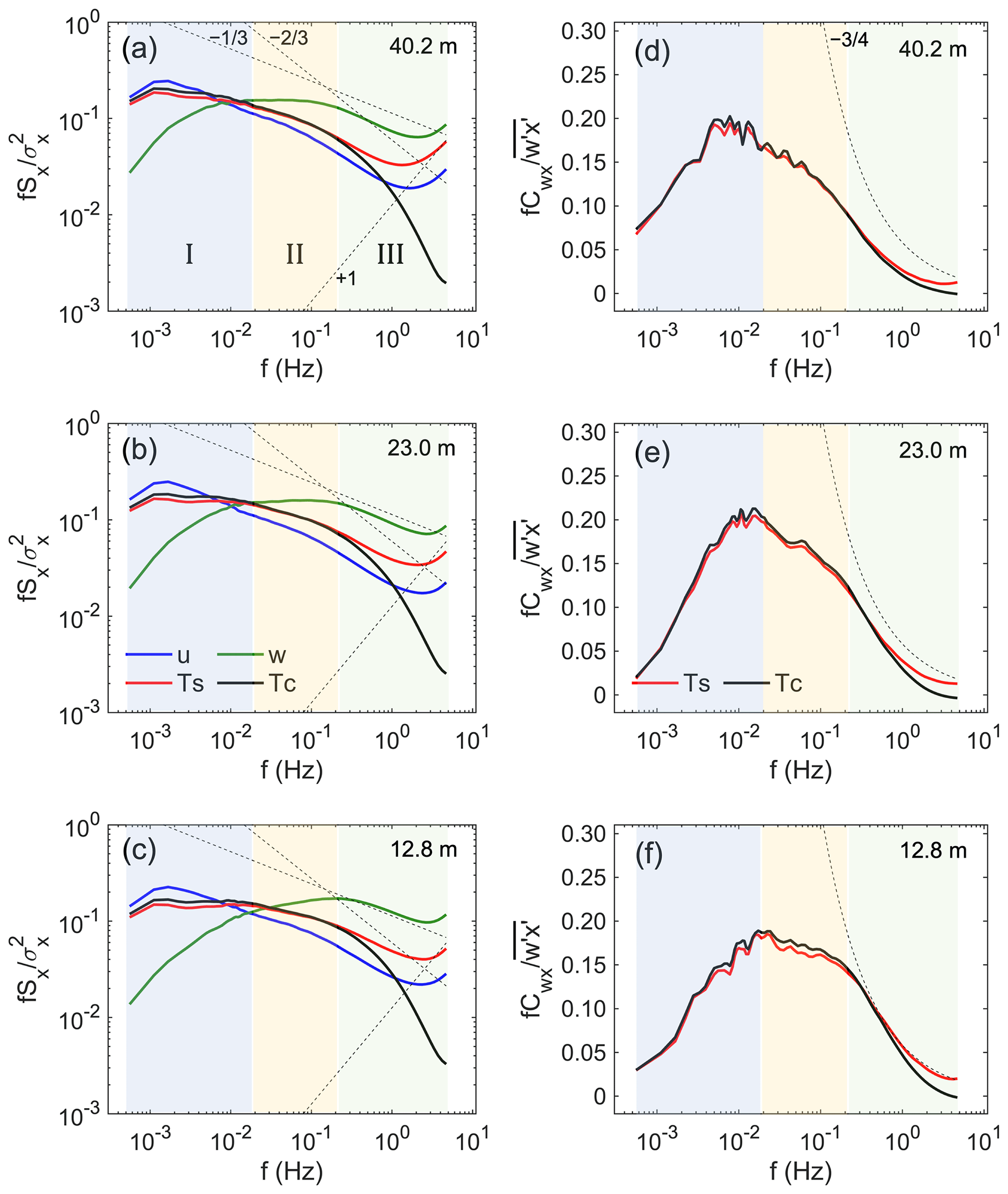
Figure 3 Mean normalized power spectra of u, w, T_s, and T_c and cospectra of w–T_s and w–T_c at the three heights of 40.2, 23.0, and 12.8 m, respectively. All power spectra and cospectra are normalized by the corresponding variance and covariance before averaging. The dashed lines show a $f^{-\mathrm{1}/\mathrm{3}}$, $f^{-\mathrm{2}/\mathrm{3}}$, f⁺¹, and $f^{-\mathrm{3}/\mathrm{4}}$ slope. Note that the frequency domain can be divided into three regions by comparing the T_s and T_c spectra.

It is also noted that the magnitude of the T_c spectra is higher than that of the T_s spectra in the low-frequency range of f < 0.02 Hz, but their magnitude is comparable in the middle-frequency range of 0.02 Hz < f < 0.2 Hz. These results indicate that turbulent eddies with scales less than 0.02 Hz contribute more to ${\mathit{\sigma }}_{T_{\mathrm{c}}}^{\mathrm{2}}$ than ${\mathit{\sigma }}_{T_{\mathrm{s}}}^{\mathrm{2}}$. Hence, the underestimation of ${\mathit{\sigma }}_{T_{\mathrm{s}}}^{\mathrm{2}}$ is mostly caused by the lower magnitude of the T_s spectra in the low-frequency range, whereas ${\mathit{\sigma }}_{T_{\mathrm{s}}}^{\mathrm{2}}$ is overestimated to some extent due to the upturned distortion of the T_s spectra in the high-frequency range.

Figure 3d–f show the distribution of the mean normalized w–T_s and w–T_c cospectra as a function of f. Each one of the cospectra is normalized by the corresponding covariances before averaging. For f > 0.2 Hz, especially when f > 0.5 Hz, the w–T_s cospectra are generally higher than the w–T_c cospectra, consistent with the higher spectra of T_s. Compared to the power law of $-\mathrm{3}/\mathrm{4}$, the calculated $\stackrel{\mathrm{‾}}{w^{\prime }{T}_{\mathrm{s}}^{\prime }}$ values are overestimated, while $\stackrel{\mathrm{‾}}{w^{\prime }{T}_{\mathrm{c}}^{\prime }}$ is slightly underestimated. For 0.002 Hz < f < 0.2 Hz, the normalized w–T_s cospectra are slightly lower than the normalized w–T_c cospectra, indicating that turbulent eddies with scales in the frequency range of 0.002 Hz < f < 0.2 Hz contribute more to $\stackrel{\mathrm{‾}}{w^{\prime }{T}_{\mathrm{c}}^{\prime }}$. Overall, the underestimation of the CSAT3B-derived fluxes is also scale-dependent, and the underestimation of $\stackrel{\mathrm{‾}}{w^{\prime }{T}_{\mathrm{s}}^{\prime }}$ in the middle- to low-frequency range is offset by the overestimation in the high-frequency range to some extent.

According to the comparison of the T_s and T_c spectra, the whole frequency domain can be divided into three ranges: (I) f < 0.02 Hz, (II) 0.02 Hz < f < 0.2 Hz, and (III) f > 0.2 Hz. For f < 0.02 Hz, the magnitude of the T_c power spectra is slightly higher than that of the T_s spectra at all levels, but the magnitude of the T_s and T_c spectra is comparable in the middle-frequency range of 0.02 Hz < f < 0.2 Hz. For f > 0.2 Hz, the T_c spectra first follow the $-\mathrm{5}/\mathrm{3}$ power law and are then attenuated, whereas the T_s spectra are distorted upward. Based on this division, in Sect. 3.3, the 30 min time series is divided into the three frequency ranges, and the contributions of these different scales to ${\mathit{\sigma }}_{T_{\mathrm{s}}}^{\mathrm{2}}$, ${\mathit{\sigma }}_{T_{\mathrm{c}}}^{\mathrm{2}}$, $\stackrel{\mathrm{‾}}{w^{\prime }{T}_{\mathrm{s}}^{\prime }}$, and $\stackrel{\mathrm{‾}}{w^{\prime }{T}_{\mathrm{c}}^{\prime }}$ at different heights are then quantified.

3.3 Scale-dependent contributions to variances and fluxes

To quantify the contributions of different scales to the corresponding temperature variances and fluxes, we apply the EEMD approach to decompose the 30 min time series of w^′, $T_{\mathrm{s}}^{\prime }$, and $T_{\mathrm{c}}^{\prime }$ into various oscillatory components, which are then categorized into the three frequency ranges discussed earlier (i.e., I, II, and III). Figure 4a–c depict that for regime I, the ratios between the variances of T_s and T_c are generally lower than 1.0 (approximately 0.89 on average). This suggests that turbulent eddies with scales less than 0.02 Hz contribute approximately 11 % more to ${\mathit{\sigma }}_{T_{\mathrm{c},\mathrm{I}}}^{\mathrm{2}}$ than ${\mathit{\sigma }}_{T_{\mathrm{s},\mathrm{I}}}^{\mathrm{2}}$. With these turbulent eddies contributing about 41 %–57 % to the total variances (Fig. 5a–c and Table 1), the 11 % difference between ${\mathit{\sigma }}_{T_{\mathrm{c},\mathrm{I}}}^{\mathrm{2}}$ and ${\mathit{\sigma }}_{T_{\mathrm{s},\mathrm{I}}}^{\mathrm{2}}$ would cause 4 %–6 % difference between the total variances of T_s and T_c. As for fluxes, turbulent eddies with scales less than 0.02 Hz contribute approximately 6 % more to ${\stackrel{\mathrm{‾}}{w^{\prime }{T}_{\mathrm{s}}^{\prime }}}_{\mathrm{I}}$ than ${\stackrel{\mathrm{‾}}{w^{\prime }{T}_{\mathrm{c}}^{\prime }}}_{\mathrm{I}}$. With these turbulent eddies accounting for about 26 %–45 % of the total fluxes (Fig. 5d–f and Table 1), the 6 % difference in ${\stackrel{\mathrm{‾}}{w^{\prime }{T}_{\mathrm{s}}^{\prime }}}_{\mathrm{I}}$ and ${\stackrel{\mathrm{‾}}{w^{\prime }{T}_{\mathrm{c}}^{\prime }}}_{\mathrm{I}}$ would cause 2 %–3 % difference in the total fluxes. Further, given that the contribution of regime I to the total temperature variances and fluxes increases with measurement height (Fig. 5 and Table 1), the underestimation becomes more significant at higher levels.

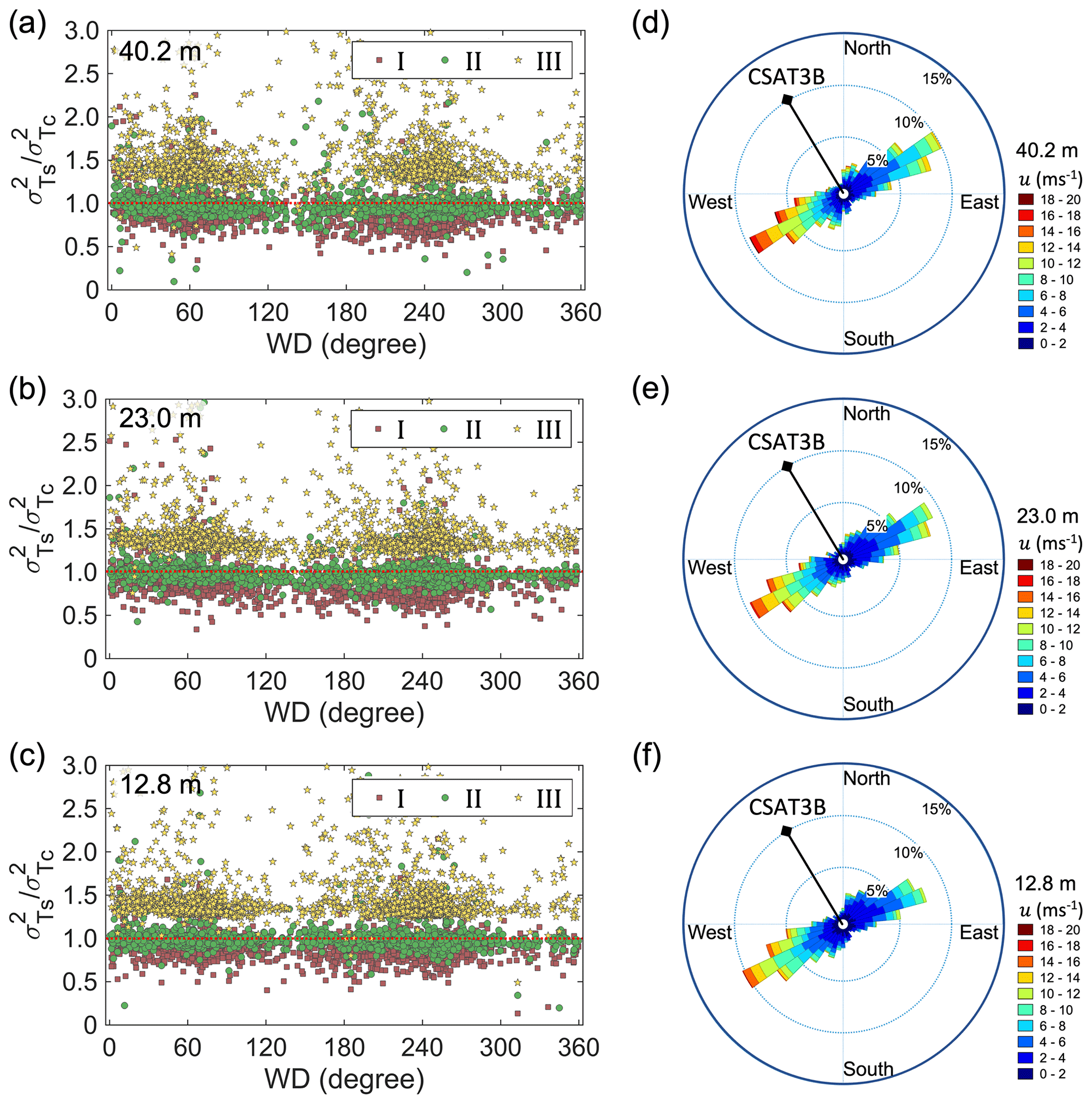
Figure 4 (a–c) Distribution of ratios of half-hourly variances of T_s and T_c with wind directions and (d–f) wind roses at the heights of 40.2, 23.0, and 12.8 m, respectively. The square, circle, and star markers represent the ratios of the variances in the three frequency ranges. The black lines in (d)–(f) refer to directions of the mounting arms of instruments.

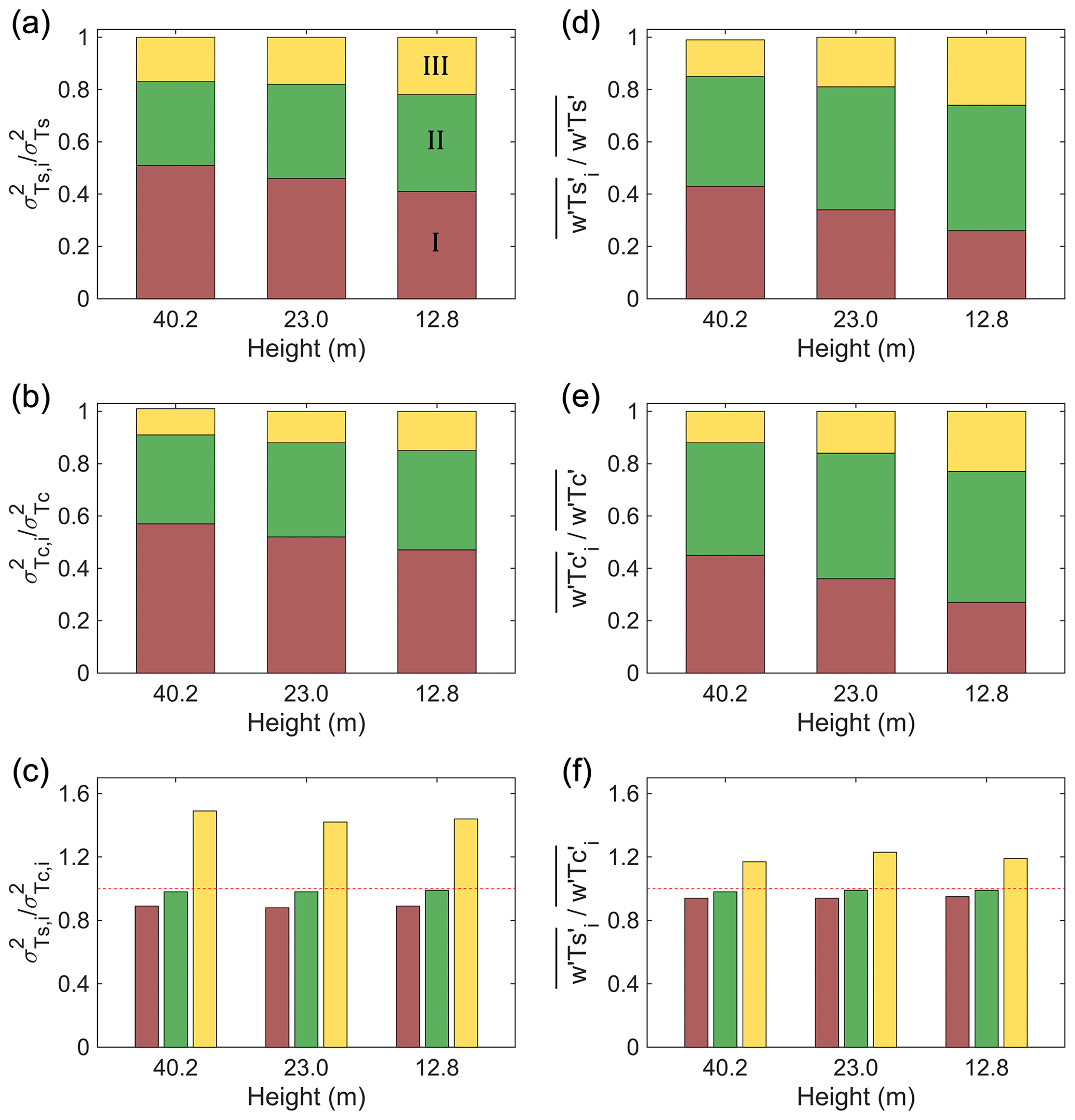
Figure 5 Contributions of the three frequency ranges to the total temperature variances and fluxes of T_s and T_c, respectively, as well as the mean ratios of the temperature variances and fluxes of T_s and T_c for each regime.

Table 1 Contributions of the three frequency ranges to the total temperature variances and fluxes of T_s and T_c, as well as the mean ratios of temperature variances and fluxes of T_s and T_c for each range.

For regime II, the ratios between the variances of T_s and T_c and the associated fluxes are close to 1.0 with minimal scatter. This indicates that turbulent eddies with scales between 0.02 and 0.2 Hz contribute consistently to the temperature variances and fluxes. These turbulent eddies contribute 32 %–38 % and 42 %–50 % to their total variances and fluxes, respectively (Fig. 5 and Table 1). For regime III, the ratios between the variances of T_s and T_c average about 1.45 at the three heights due to the distorted spectra in this regime for both T_s and T_c. This indicates that turbulent eddies with scales larger than 0.2 Hz contribute roughly 45 % less to ${\mathit{\sigma }}_{T_{\mathrm{c},\text{III}}}^{\mathrm{2}}$ than ${\mathit{\sigma }}_{T_{\mathrm{s},\text{III}}}^{\mathrm{2}}$. With these turbulent eddies contributing about 12 %–26 % to the total variances (Fig. 5a–c and Table 1), the 45 % difference in ${\mathit{\sigma }}_{T_{\mathrm{c},\text{III}}}^{\mathrm{2}}$ and ${\mathit{\sigma }}_{T_{\mathrm{s},\text{III}}}^{\mathrm{2}}$ would cause 5 %–7 % difference in the total variances of T_s and T_c. As for fluxes, turbulent eddies with scales larger than 0.2 Hz contribute approximately 20 % less to ${\stackrel{\mathrm{‾}}{w^{\prime }{T}_{\mathrm{c}}^{\prime }}}_{\text{III}}$ than ${\stackrel{\mathrm{‾}}{w^{\prime }{T}_{\mathrm{s}}^{\prime }}}_{\text{III}}$. With these turbulent eddies accounting for 12 %–26 % of the total fluxes (Fig. 5d–f and Table 1), the 20 % difference in ${\stackrel{\mathrm{‾}}{w^{\prime }{T}_{\mathrm{c}}^{\prime }}}_{\text{III}}$ and ${\stackrel{\mathrm{‾}}{w^{\prime }{T}_{\mathrm{s}}^{\prime }}}_{\text{III}}$ would cause 2 %–4 % difference in the total fluxes. These results suggest that the observed underestimation of the T_s variances and fluxes is primarily attributed to the large turbulent eddies with frequencies less than 0.02 Hz, which is offset to some extent by the contribution from small turbulent eddies with frequencies larger than 0.2 Hz.

3.4 Potential causes for the scale-dependent differences

The potential causes for the scale-dependent differences between the T_s and T_c spectra are measurement errors, solar heating of thermocouples, and tower and mounting arm vibrations, among others (e.g., the deficiency in the design of sonic anemometers in response to different wind speed conditions). The T_c spectra follow similar declining features in the high-frequency range independent of wind speed (Text S2 and Fig. S2 in the Supplement), suggesting that measurements of the fine-wire thermocouples were not noticeably affected by increased wind speed, and therefore operational errors could be excluded from the causes for the observed difference. Additionally, the consistent differences between the power spectra of T_s and T_c under nighttime and daytime conditions (Text S1 and Fig. S1) suggest that the impact of solar heating on thermocouples was also not the cause for the differences between the T_s and T_c variances and fluxes.

Figure 6 Power spectra of (a) the sonic roll angles and (b) the sonic pitch angles measured by CSAT3B at the three heights. The sonic roll and pitch angles were stored as 30 min averages during the experiment.

As the wind speed increases, the tower vibrations become more pronounced, especially at higher levels, as indicated by the more energetic peaks in the power spectra of sonic roll and pitch angles (Fig. 6). For wind speed below approximately 10 m s⁻¹ at 40.2 m, the ratios of the T_s and T_c variances for regime I show no obvious change with wind speed. However, for wind speed above 10 m s⁻¹, the ratios decrease further as wind speed increases (Fig. 7a). The ratios of the temperature fluxes of T_s and T_c exhibit a similar pattern to the variances (Fig. 7d). For regime II, the ratios of both the variance and fluxes of T_s and T_c show no obvious relations with wind speed (Fig. 7b and e). For regime III, the ratios of both the variance and fluxes of T_s and T_c illustrate large scatter, especially when wind speed is below 10 m s⁻¹, but still show no obvious trends as wind speed increases (Fig. 7c and f).

Figure 7 Ratios of (a–c) half-hourly variances of T_s and T_c and (d–f) covariances of w–T_s and w–T_c corresponding to the low-, middle-, and high-frequency ranges, respectively, as a function of the mean wind speed ($\stackrel{\mathrm{‾}}{u}$) at 40.2 m.

We thus hypothesize that the enhanced tower vibrations under strong winds lead to an early or delayed detection of the sonic pulse. This results in overestimations or underestimations of the speed of sound and thus errors in the 10 Hz time series of sonic temperature. In this study, for wind speeds below 10 m s⁻¹, the ratios of the variances (and fluxes) of T_s to those of T_c are scattered around 1.0 for regime I. However, for wind speed above 10 m s⁻¹, the ratios decrease as wind speed further increases (Fig. 7). Therefore, tower and mounting arm vibrations were most likely the cause for the differences in the temperature variance and fluxes. Under this circumstance, such vibrations may also affect sonic-measured wind components along with T_s, resulting in errors in all the calculated fluxes. However, rigorous tests of this hypothesis seem necessary through testing sonic anemometers in wind tunnels or fields with different mounting strategies.

3.5 Implications for water vapor and CO₂ fluxes

Given that Eqs. (2) and (3) are used to adjust the measured densities of water vapor and CO₂ by open-path CO₂–H₂O gas analyzers in EC systems, any errors in temperature measurements would be propagated to water vapor and CO₂ time series through these two equations. In Eqs. (2) and (3), T_s can be replaced by T_c to achieve the adjusted time series of densities of water vapor and CO₂ for FW3. The adjusted time series of water vapor and CO₂ by the fluctuating parts of T_s and T_c, respectively, are then decomposed into three frequency ranges to quantify the influence of T_s on variances and fluxes of water vapor and CO₂.

The variances of ρ_v are not influenced by the use of either T_s or T_c for the density effect corrections (Table S1 in the Supplement) because the fluctuations in ρ_v are not very sensitive to density effects, especially at semiarid sites like ours (Gao et al., 2020). Therefore, for the water vapor fluxes, there are only minor differences (< 1 %) between the fluxes corrected by T_s and T_c for the three frequency ranges, while the overall water vapor fluxes corrected by T_s and T_c are comparable at the three heights (Fig. 8a–c).

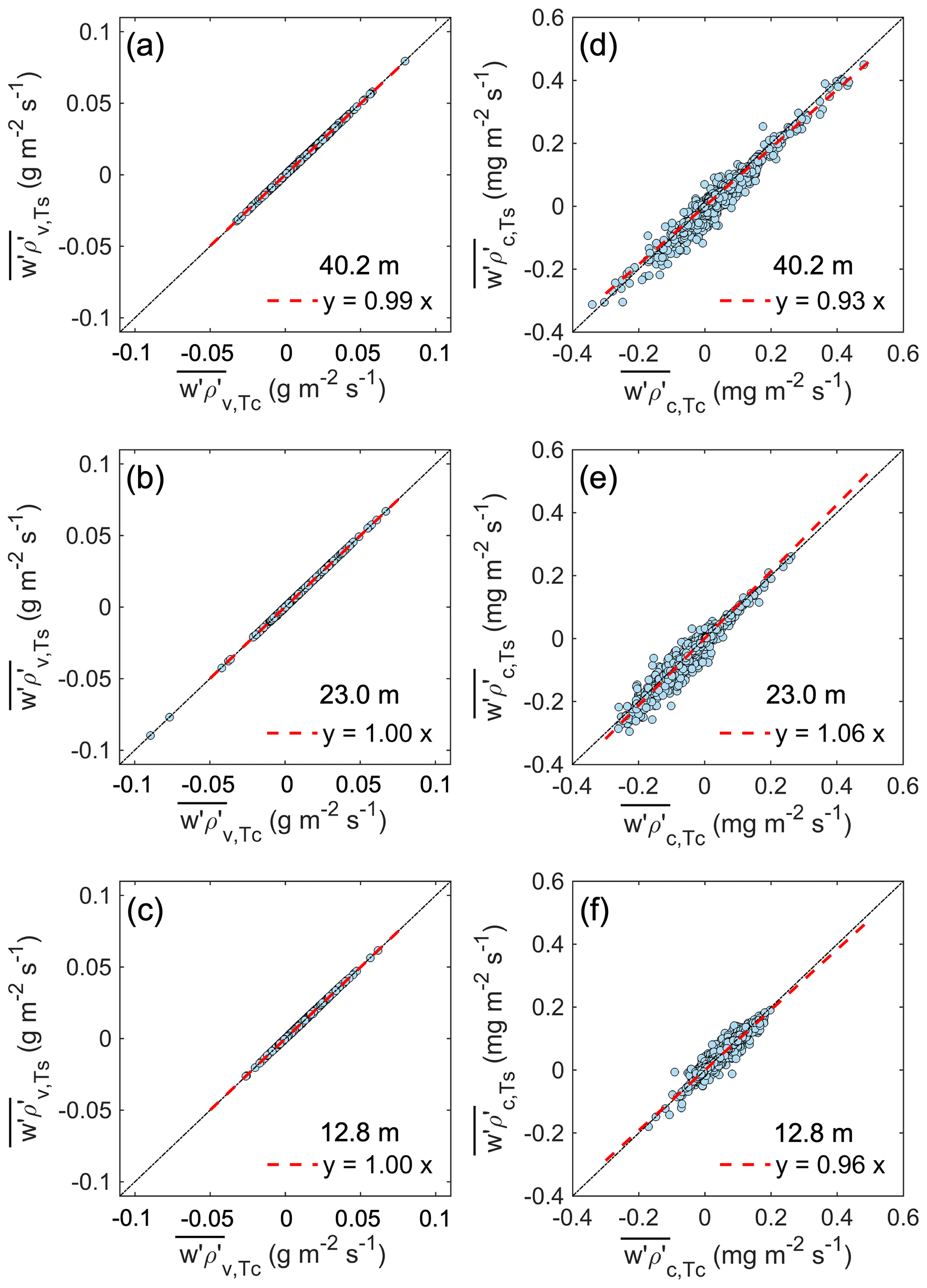
Figure 8 Comparison of water vapor and CO₂ fluxes corrected by temperature from sonic anemometers and fine-wire thermocouples, respectively, at the three heights.

As for CO₂, the differences between T_s and T_c in the three frequency ranges are propagated differently to the adjusted variances of ρ_c (Table S2 in the Supplement). More importantly, there are relatively large differences (but still within 10 %) between the CO₂ fluxes adjusted by T_s and T_c (Fig. 8d–f). In general, CO₂ fluxes are more sensitive to errors or uncertainties in temperature measurements than water vapor fluxes (Liu et al., 2006). Therefore, precise measurements of air temperature are critical for quantifying ecosystem CO₂ fluxes.

4 Conclusions

Temperature variances and the associated fluxes are examined using sonic anemometers and co-located fine-wire thermocouples at three levels above a sagebrush ecosystem. Compared to temperature variances and fluxes determined by thermocouples, sonic anemometers were found to underestimate the variances and fluxes by approximately 5 % and 4 %, respectively, at the height of 40.2 m. In the high-frequency range, the distortion in T_s spectra contributed to the heat fluxes by 2 %–4 %, whereas the attenuation in T_c spectra led to underestimated fluxes. However, the primary source of the underestimation in temperature variances and fluxes by the sonic anemometers was identified in the low- frequency range. This phenomenon became more profound with increasing wind speed and, thus, heightened vibrations of the tower and mounting arms. Furthermore, when adjusting the density effects using the attenuated temperature, our results indicate that CO₂ variances and fluxes are more sensitive to errors or uncertainties in temperature measurements compared to those of water vapor at the semiarid site.

Our findings highlight the critical importance of accurate measurements of air temperature fluctuations in EC flux measurements. The inclusion of additional high-frequency temperature measurements using fine-wire thermocouples is thus strongly recommended for EC systems. Furthermore, the observed underestimation of sonic temperature variances and fluxes suggests that the measured wind velocity components may also be biased due to the tower vibrations. Therefore, we recommend further investigation of the influence of mounting arm vibrations on wind velocity components by sonic anemometers.