Retrieval and analysis of the composition of an aerosol mixture through Mie–Raman–fluorescence lidar observations

In the atmosphere, aerosols can originate from numerous sources, leading to the mixing of different particle types. This paper introduces an approach to the partitioning of aerosol mixtures in terms of backscattering coefficients. The method utilizes data collected from the Mie–Raman–fluorescence lidar, with the primary input information being the aerosol backscattering coefficient (β), particle depolarization ratio (δ), and fluorescence capacity (G_F). The fluorescence capacity is defined as the ratio of the fluorescence backscattering coefficient to the particle backscattering coefficient at the laser wavelength. By solving a system of equations that model these three properties (β, δ and G_F), it is possible to characterize a three-component aerosol mixture. Specifically, the paper assesses the contributions of smoke, urban, and dust aerosols to the overall backscattering coefficient at 532 nm. It is important to note that aerosol properties (δ and G_F) may exhibit variations even within a specified aerosol type. To estimate the associated uncertainty, we employ the Monte Carlo technique, which assumes that G_F and δ are random values uniformly distributed within predefined intervals. In each Monte Carlo run, a solution is obtained. Rather than relying on a singular solution, an average is computed across the whole set of solutions, and their dispersion serves as a metric for method uncertainty. This methodology was tested using observations conducted at the ATOLL (ATmospheric Observation at liLLe) observatory, Laboratoire d'Optique Atmosphérique, University of Lille, France.

1 Introduction

Studying the physicochemical properties of atmospheric aerosols is crucial for understanding their impact on Earth's radiation balance and climate. To simplify the complexity of aerosol composition, it is essential to classify aerosol types. Categorization of aerosols into several basic types, e.g., urban, dust, marine, and biomass burning (Dubovik et al., 2002), allows the range of variability of observed aerosol parameters to be covered and the analysis and interpretation of aerosol data to be facilitated. The multiwavelength Mie–Raman and HSRL (High Spectral Resolution Lidar) lidar systems provide a unique opportunity to derive height-resolved particle intensive properties, such as Ångström exponents, lidar ratios, and depolarization ratios at multiple wavelengths. These properties can be used as inputs for classification schemes (Burton et al., 2012, 2013; Groß et al., 2013; Mamouri and Ansmann, 2017; Papagiannopoulos et al., 2018; Nicolae et al., 2018; Hara et al., 2018; Voudouri et al., 2019; Wang et al., 2021; Mylonaki et al., 2021; Wandinger et al., 2023; Floutsi et al., 2024). However, aerosols in the atmosphere often originate from multiple sources, leading to the mixing of different particle types. To understand the impact of different aerosol types within a mixture, it is necessary to quantify the content of each type.

In the cases involving mixtures of two aerosol types with significantly different depolarization ratios, the partitioning of aerosol backscattering coefficients becomes straightforward (Sugimoto and Lee, 2006; Tesche et al., 2009; Miffre et al., 2020). Burton et al. (2014) formulated the mixing rules for several aerosol intensive parameters, such as the lidar ratio, backscatter color ratio, and depolarization ratio, and applied these rules to two-component aerosol mixtures. However, the partition becomes increasingly challenging when dealing with more than two types of particles. The limited number of lidar-measured intensive particle properties specific to individual aerosol types contributes to this challenge. Even for a single aerosol type, the measured particle parameters, such as lidar ratios, demonstrate a wide range of variability (Floutsi et al., 2023). Distinguishing between urban and smoke particles poses a particular challenge as these two types exhibit similar lidar-measured properties (Floutsi et al., 2023). Therefore, additional independent information is needed to enhance the characterization of aerosol parameters.

Independent information about aerosol properties can be obtained through fluorescence lidar measurements (Reichardt et al., 2018, 2023; Veselovskii et al., 2020; Zhang et al., 2021). The fluorescence lidar allows the fluorescence backscattering coefficient β_F to be evaluated, which is derived from the ratio of fluorescence and nitrogen Raman backscatters (Veselovskii et al., 2020). The particle intensive property in fluorescence lidar measurements is the fluorescence capacity G_F, which is the ratio of β_F to the aerosol backscattering coefficient at the laser wavelength. The fluorescence capacity of smoke is approximately 1 order higher than that of urban particles, providing a basis for distinguishing between these two aerosol types (Veselovskii et al., 2022). Additionally, recent studies have shown that a classification scheme relying on two intensive parameters – the particle depolarization ratio at 532 nm (δ₅₃₂) and the fluorescence capacity, effectively separates four aerosol types: dust, smoke, pollen, and urban, as demonstrated in the publication of Veselovskii et al. (2022). It is noteworthy that the classification scheme in that paper does not discriminate particles based on their absorption properties, so the “urban” type encompasses both continental aerosol and anthropogenic pollution. Furthermore, maritime aerosol is not included in the classification at present, as the lidar observations were performed over Lille, where maritime particles are not prevalent (though the possibility of its inclusion is acknowledged).

The algorithm presented in the study of Veselovskii et al. (2022) showcases the capability to perform aerosol classification with high spatiotemporal resolution. However, as mentioned earlier, it is essential to quantify the content of the mixture. In this study, we extended the approach beyond classification to partition aerosol mixtures in terms of the backscattering coefficients of basic aerosol types. To test the algorithm, we analyzed observations at the ATOLL (ATmospheric Observation at liLLe) at Laboratoire d'Optique Atmosphérique, University of Lille, between 2020 and 2023, performed during periods of strong smoke and dust episodes. We begin by providing a description of the lidar system (Sect. 2.1), and in Sect. 2.2, a novel approach for mixture partitioning is presented. In the “Application of the partition algorithm to lidar observations” section (Sect. 3), we present three case studies that demonstrate how the algorithm operates. The paper concludes with a summary of our findings in the Conclusion section.

2 Experimental setup and approach for aerosol mixture partitioning

2.1 Lidar system

The Mie–Raman–fluorescence lidar LILAS (LIlle Lidar AtmosphereS) is equipped with a tripled Nd:YAG laser that operates at a repetition rate of 20 Hz and has a pulse energy of approximately 100 mJ at 355 nm. A 40 cm aperture Newtonian telescope is utilized to collect the backscattered light, and Licel transient recorders with a range resolution of 7.5 m are employed to digitize the lidar signals. This configuration allows for simultaneous detection in both analog and photon counting modes. The objective of the LILAS system is to detect elastic and Raman backscattering, which enables the measurement of various properties through the $\mathrm{3}\mathit{\beta }+\mathrm{2}\mathit{\alpha }+\mathrm{3}\mathit{\delta }$ data configuration. This includes three particle backscattering coefficients (β₃₅₅, β₅₃₂, β₁₀₆₄), two extinction coefficients (α₃₅₅, α₅₃₂), and three particle depolarization ratios (δ₃₅₅, δ₅₃₂, δ₁₀₆₄). The particle depolarization ratio, determined as a ratio of cross- and co-polarized components of the particle backscattering coefficient, was calculated and calibrated in the same way as described in Freudenthaler et al. (2009). Additionally, the LILAS system is capable of profiling the laser-induced fluorescence of aerosol particles. This is achieved using a wideband interference filter with a width of 44 nm, centered at 466 nm, as suggested by Veselovskii et al. (2020). Due to the strong sunlight background during daytime, the fluorescence observations are limited to nighttime hours.

The calculation of the fluorescence capacity G_F can be performed using backscattering coefficients at any laser wavelength. In our study, we specifically used β₅₃₂, as it is determined using rotational Raman scattering and is considered to be the most reliable; thus $G_{\mathrm{F}}=\frac{{\mathit{\beta }}_{\mathrm{F}}}{{\mathit{\beta }}_{\mathrm{532}}}$. To supplement our measurements, additional information about atmospheric properties was obtained from radiosonde measurements conducted at Herstmonceux (UK) and Beauvechain (Belgium) stations, which are located approximately 160 and 80 km away from the observation site, respectively. The lidar measurements were primarily conducted vertically. In cases where observations were made at an angle to the horizon, the corresponding information has been included in the captions of the figures.

2.2 Approach for mixture partitioning

The lidar system measures up to nine independent properties of aerosols. However, our main focus is on the separation of the backscatters of individual aerosol types with high spatiotemporal resolution. To calculate parameters related to the extinction coefficient, such as the lidar ratio or extinction Ångström exponent, it is necessary to average lidar profiles over a substantial spatiotemporal interval. In this study, as a first step, we use three parameters with high resolution in both height and temporal domains: the backscattering coefficient β₅₃₂, the depolarization ratio δ₅₃₂, and the fluorescence capacity G_F. Moreover, the calculation process partially cancels out the overlap functions, allowing us to derive β₅₃₂, δ₅₃₂, and G_F closer to the ground compared to aerosol extinction. We are considering a scenario where only three externally mixed aerosol types occur, such as smoke (s), dust (d), and urban (u). The aerosol and fluorescence backscattering coefficients (β₅₃₂ and β_F) are the sum of their respective contributions.

$$\begin{array}{}\text{(1)}& {\displaystyle }{\mathit{\beta }}_{\mathrm{532}}={\mathit{\beta }}_{\mathrm{532}}^{\mathrm{s}}+{\mathit{\beta }}_{\mathrm{532}}^{\mathrm{d}}+{\mathit{\beta }}_{\mathrm{532}}^{\mathrm{u}}\text{(2)}& {\displaystyle }{\mathit{\beta }}_{\mathrm{F}}={\mathit{\beta }}_{\mathrm{F}}^{\mathrm{s}}+{\mathit{\beta }}_{\mathrm{F}}^{\mathrm{d}}+{\mathit{\beta }}_{\mathrm{F}}^{\mathrm{u}}\end{array}$$

The fluorescence capacities for each aerosol type are

$$\begin{array}{}\text{(3)}& G_{\mathrm{F}}^i={\displaystyle \frac{{\mathit{\beta }}_{\mathrm{F}}^i}{{\mathit{\beta }}_{\mathrm{532}}^i}},\end{array}$$

where i= s, d, u. The fractions of β₅₃₂ for individual aerosol types are

$$\begin{array}{}\text{(4)}& {\mathit{\eta }}_i={\displaystyle \frac{{\mathit{\beta }}_{\mathrm{532}}^i}{{\mathit{\beta }}_{\mathrm{532}}}}.\end{array}$$

By definition,

$$\begin{array}{}\text{(5)}& {\mathit{\eta }}_{\mathrm{s}}+{\mathit{\eta }}_{\mathrm{d}}+{\mathit{\eta }}_{\mathrm{u}}=\mathrm{1}.\end{array}$$

The fluorescence capacity can be expressed as a linear combination of the fluorescence capacities of each aerosol type, as shown in Eq. (6):

$$\begin{array}{}\text{(6)}& G_{\mathrm{F}}={\mathit{\eta }}_{\mathrm{s}}{G}_{\mathrm{F}}^{\mathrm{s}}+{\mathit{\eta }}_{\mathrm{d}}{G}_{\mathrm{F}}^{\mathrm{d}}+{\mathit{\eta }}_{\mathrm{u}}{G}_{\mathrm{F}}^{\mathrm{u}}.\end{array}$$

The particle depolarization ratio is a ratio of the cross- and co-polarized component of the backscattering coefficient: ${\mathit{\delta }}_{\mathrm{532}}=\frac{{\mathit{\beta }}_{\mathrm{532}}^{\perp }}{{\mathit{\beta }}_{\mathrm{532}}^{\parallel }}$. However, for the mixture analysis, the use of the depolarization potential ${\mathit{\delta }}_{\mathrm{532}}^{\prime }=\frac{{\mathit{\delta }}_{\mathrm{532}}}{\mathrm{1}+{\mathit{\delta }}_{\mathrm{532}}}$ is preferable because δ^′, the same as G_F, is a linear combination of the depolarization potentials of individual particle types (${\mathit{\delta }}_{\mathrm{532}}^{\prime \mathrm{s}}$, ${\mathit{\delta }}_{\mathrm{532}}^{\prime \mathrm{d}}$, ${\mathit{\delta }}_{\mathrm{532}}^{\prime \mathrm{u}}$), as outlined by Burton et al. (2014).

$$\begin{array}{}\text{(7)}& {\mathit{\delta }}_{\mathrm{532}}^{\prime }={\mathit{\eta }}_{\mathrm{s}}{\mathit{\delta }}_{\mathrm{532}}^{\prime \mathrm{s}}+{\mathit{\eta }}_{\mathrm{d}}{\mathit{\delta }}_{\mathrm{532}}^{\prime \mathrm{d}}+{\mathit{\eta }}_{\mathrm{u}}{\mathit{\delta }}_{\mathrm{532}}^{\prime \mathrm{u}}\end{array}$$

Finally, we have a system of three equations, Eqs. (5)–(7), from which we can determine the relative contributions of each aerosol type by finding η_s, η_d, and η_u. In our study, we solve the system (Eqs. 5–7) using the least-squares method with an additional constraint on the non-negativity of solutions. As mentioned earlier, the particle parameters may vary within predetermined ranges, even for a specific aerosol type. However, the exact values of $G_{\mathrm{F}}^i$ and ${\mathit{\delta }}_{\mathrm{532}}^{\prime }$ at a specific height–time pixel are unknown. To address the uncertainty in η_i, we employ the Monte Carlo technique, assuming that $G_{\mathrm{F}}^i$ and ${\mathit{\delta }}_{\mathrm{532}}^{\prime }$ are random values uniformly distributed within the predetermined intervals. For each Monte Carlo trial, random values of $G_{\mathrm{F}}^i$ and ${\mathit{\delta }}_{\mathrm{532}}^{\prime }$ are generated. Instead of relying on a single solution, we conduct a series of Monte Carlo trials in order to obtain a set of solutions and calculate the average of this set. The dispersion of these solutions is taken as a measure of method uncertainty. The number of Monte Carlo trials was set to 100, and further increase in this number did not significantly impact either the final average or the dispersion of solutions. In our classification scheme, we include four types of aerosols (smoke, pollen, urban, dust). Nevertheless, the system of equations (Eqs. 5–7) consists of only three equations. Given that it is highly unlikely to have all four aerosol types coexisting at a single height–time pixel, one of the four types can be excluded a priori based on a G_F–δ₅₃₂ diagram or other pertinent considerations. Another option is to exclude one aerosol type at each height–time pixel based on the lidar data itself, as described below. We will call such a method automatic type selection (ATS).

For ATS, we solve the system given by Eqs. (5)–(7) for the triplets (S, P, U), (S, P, D), (S, D, U), and (P, D, U), where S, D, U, and P denote smoke, dust, urban, and pollen, respectively. To determine which aerosol types can be excluded, we use the discrepancy for Eqs. (6) and (7) as a criterion. Specifically, we calculate the difference between the input data (G_F–δ₅₃₂) and the corresponding values obtained by substituting the solution into the right-hand side of Eqs. (6) and (7). The aerosol triplet that provides the least discrepancy is chosen for this single Monte Carlo trial and for the height–time pixel. This procedure is repeated for every Monte Carlo trial, and after averaging, the spatiotemporal distributions of η_s, η_p, η_u, and η_d are evaluated.

3 Application of the partition algorithm to lidar observations

3.1 Range of particle parameters used in the inversion scheme

The uncertainty of the partitioning of backscattering coefficients depends on the range of G_F and δ₅₃₂ variations in each aerosol type. To establish this range, we analyzed measurement sessions at the ATOLL for the period of 2020–2023. Our focus was on observation episodes characterized by stable atmospheric conditions, where only a single aerosol type predominated, at least within specific height–time intervals. Moreover, we took precautions to ensure that the relative humidity in the selected intervals remained below 60 % to minimize the impact of particle hygroscopic growth. The example of such an impact is presented in Fig. 6 of Veselovskii et al. (2024). Based on the obtained results, we summarized the ranges of parameter variation in Table 1. The ranges are slightly different from the ones in Table 1 of Veselovskii et al. (2022) because since that publication, numerous observations have been performed, providing more material for analysis. The depolarization ratios δ₅₃₂ for smoke and urban particles fall within the range of 2 %–8 %, while for dust, this range is 25 %–35 %. The depolarization ratio of long transported dust can be lower, but at this stage, we do not consider possible modifications of dust properties during transportation. We attribute lower values of δ₅₃₂ to the mixing of dust with pollutants (urban aerosol in our model). It should be mentioned that the depolarization ratio of smoke in the upper troposphere can be as high as 20 % (Ohneiser et al., 2020); however, in the low and middle troposphere, where partitioning was performed, we limited δ₅₃₂ to a value of 8 %.

Table 1 Variation ranges of fluorescence capacity and the particle depolarization ratio for different types of aerosols.

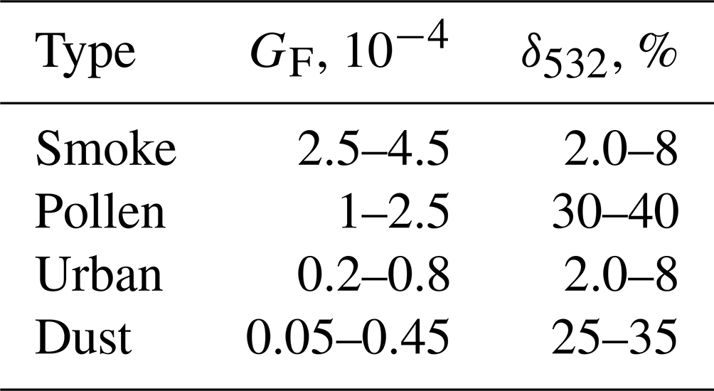
The fluorescence capacity of smoke is high due to the presence of organic carbon. In the upper troposphere, G_F can reach $\mathrm{10}\times {\mathrm{10}}^{-\mathrm{4}}$ (Veselovskii et al., 2024), but below 8 km, it mainly falls within the range of (2.5–4.5) $\times {\mathrm{10}}^{-\mathrm{4}}$. For dust and urban particles, the values of fluorescence capacities are within the intervals of (0.05–0.45) $\times {\mathrm{10}}^{-\mathrm{4}}$ and (0.2–0.8) $\times {\mathrm{10}}^{-\mathrm{4}}$, respectively. Determining the ranges of δ₅₃₂ and G_F for pollen is particularly challenging because, in the north of France, pollen is commonly mixed with other aerosol types. Moreover, the depolarization of pollen particles varies significantly from one type to another (Cao et al., 2010). In the Lille area, one dominant taxon is birch (Veselovskii et al., 2021) with a depolarization ratio of δ₅₃₂ at around 30 % (Cholleton et al., 2022). In our analysis, the depolarization ratio is set within the 30 %–40 % interval. The pollen consists of biological materials, and its fluorescence capacity is higher than that of urban particles. From our measurements, the variation range of G_F for pollen is estimated to be within (1.0–2.5) $\times {\mathrm{10}}^{-\mathrm{4}}$.

Below, we present three examples of applying the described approach to measurements performed at the ATOLL observatory.

3.2 Episode on 27–28 March 2022: three types of particles are observed within different spatiotemporal domains

The spatiotemporal distributions of the aerosol backscattering coefficient β₅₃₂, the particle depolarization ratio δ₅₃₂, and the fluorescence capacity G_F on 27–28 March 2022 are shown in Fig. 1. Relative humidity decreased with height, ranging from 70 % at 600 m to 55 % at 1800 m. Aerosols were primarily found below 2500 m, with several distinguishable particle types identified. The particle depolarization ratio increased to 30 % at 2000 m during the 20:00–22:00 UTC period, indicating the presence of dust. Additionally, high values of the fluorescence capacity (up to $\mathrm{2.5}\times {\mathrm{10}}^{-\mathrm{4}}$) for the 00:00–05:00 UTC period suggest the presence of smoke.

Figure 1 Spatiotemporal distributions of (a) the backscattering coefficient at 532 nm, (b) the particle depolarization ratio at 532 nm, and (c) the fluorescence capacity during the night of 27–28 March 2022. The depolarization ratio and fluorescence capacity are only calculated for the values β₅₃₂ > 0.1 Mm⁻¹ sr⁻¹. The measurements were taken at an angle of 45° to the horizon.

Figure 2a presents the G_F–δ₅₃₂ diagram for these measurements (Veselovskii et al., 2022). The red boxes represent the parameter ranges used for aerosol classification, which are slightly broader than those outlined in Table 1 to account for mixtures where one type is predominant. Dust, smoke, and urban particles can be distinguished on the diagram, together with intervals indicating mixed particle types. Although March is typically a pollen season in Lille, pollen particles did not significantly contribute to the observed episode. Utilizing this classification scheme, we assess the spatiotemporal distribution of aerosol types in Fig. 2b, following the methodology outlined in Veselovskii et al. (2022). Regions predominated by dust, smoke, and urban particles are clearly identified. A small amount of pollen is observed towards the end of the session at approximately 700 m height. The grey color in Fig. 2b represents aerosol mixtures where the particle type cannot be definitively identified. The aerosol classification presented in Fig. 2b finds support in the results of the HYSPLIT backward trajectory analysis (Stein et al., 2015) depicted in Fig. 3. Specifically, the air masses below 1000 m height were transported over Belgium, and the presence of urban aerosol is expected. Conversely, the air masses above 1500 m were transported over regions with extensive forest fires in Greece, suggesting a potential mixture of smoke and dust.

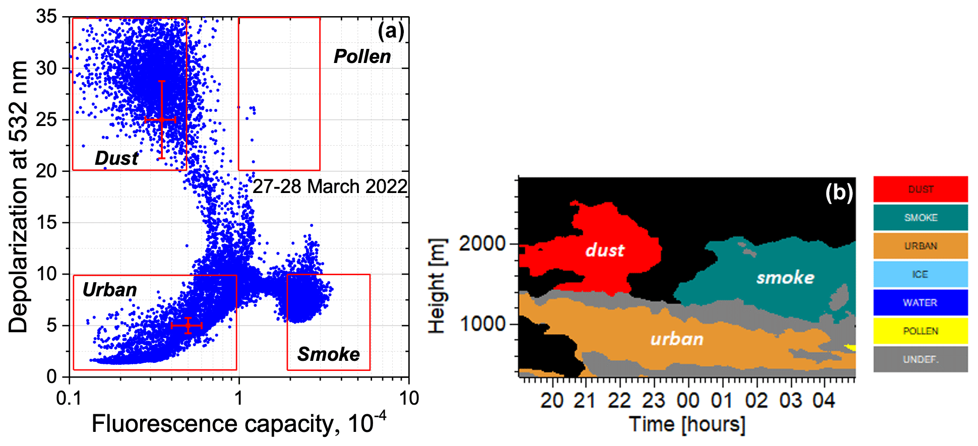
Figure 2 (a) The δ₅₃₂–G_F diagram for observations in the height range of 350–2800 m and (b) the spatiotemporal distribution of aerosol types during the night of 27–28 March 2022.

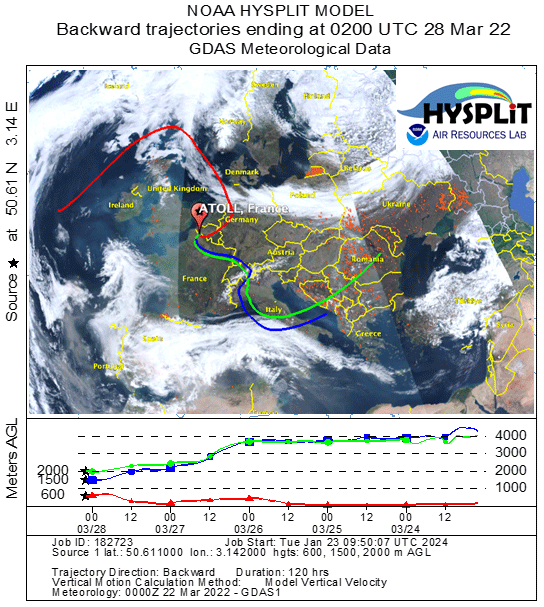
Figure 3 The HYSPLIT 5 d backward trajectories for the air mass over Lille at altitudes 600, 1500, and 2000 m on 28 March 2022 at 02:00 UTC. Red dots depict the regions of forest fires.

By applying the partition technique described in Sect. 2.2, we can determine the contribution of each particle type to the total backscattering coefficient β₅₃₂.The spatiotemporal distributions of η_s, η_u, and η_d in Fig. 4 were assessed assuming that pollen contribution can be neglected. The algorithm operates smoothly, showing distributions without any unrealistic high-frequency oscillations. By observing the distributions, it can be concluded that the smoke plume actually contains a significant amount of urban aerosol, while the dust plume does not show the presence of other particle types.

Figure 4 Relative contributions of (a) smoke (η_s), (b) urban (η_u), and (c) dust (η_d) particles to the backscattering coefficient β₅₃₂ during the night of 27–28 March 2022.

The distributions in Fig. 4 represent the mean values of η_s, η_u, and η_d. To understand the uncertainty caused by potential variations in particle characteristics, Fig. 5 displays the vertical profiles of η_s, η_u, and η_d for the period between 21:00 and 22:00 UTC, along with the corresponding standard deviations. Urban particles are predominant below 1000 m with a deviation from the mean value of roughly 5 %. Above 1500 m, η_u decreases to 0.05, and the uncertainty increases to 100 %. Conversely, dust can be disregarded below 1000 m but becomes predominant above 1000 m. Smoke contribution during the considered time period is low and only becomes noticeable (η_s ∼ 0.15) in the 1250–1500 m range. As mentioned earlier, the results in Fig. 4 were obtained without considering pollen. To assess the potential impact of pollen on the results, the partition was carried out for four aerosol types using the ATS approach, as described in Sect. 2.2. The corresponding profiles of η_s,4, η_u,4, and η_d,4 are depicted in Fig. 5 with magenta lines. Notably, the profiles obtained for three and four aerosol types are similar. Pollen does have some effect on smoke contribution (η_s decreased from 0.14 to 0.1), but its influence on dust and urban particle contribution is negligible.

Figure 5 Vertical profiles of the relative contributions of smoke (η_s), urban (η_u), and dust (η_d) particles to the backscattering coefficient β₅₃₂ on 27 March 2022. These profiles are derived under the assumption that only three aerosol types occur. The black lines depict the deviation of solutions from the mean value (η_i ± σ_i). Magenta lines show the relative contributions of smoke, urban, and dust particles (η_s,4, η_s,4, η_s,4) when four aerosol types (including pollen) are considered.

3.3 Episode on 1–2 October 2023: different types of aerosol form the layer structure

Observations at ATOLL in 2023 were notable for frequent intensive smoke events. North American wildfire smoke, transported over the Atlantic, was observed from mid-May until October. In some autumn episodes, smoke descended from the troposphere to the ground level. One such episode is shown in Fig. 6, which presents the spatiotemporal distributions of β₅₃₂, δ₅₃₂, and G_F during the night of 1–2 October 2023. During this period, the relative humidity decreased with height, from 50 % at 500 m to 30 % at 3500 m. Strong aerosol layers were observed up to 5 km in height, and the depolarization ratio δ₅₃₂ exceeded 25 % above 2000 m, indicating the predominance of dust. However, below 1000 m, a low depolarization ratio (δ₅₃₂ < 8 %) was accompanied by a high fluorescence capacity of particles (up to $\mathrm{3.0}\times {\mathrm{10}}^{-\mathrm{4}}$), identifying them as smoke. The G_F–δ₅₃₂ diagram in Fig. 7a highlights the pixels attributed to dust, smoke, and urban particles. There are also intervals where these types were mixed. These regions with mixed aerosols are represented by the grey color in the distribution of particle types in Fig. 7b. The results of aerosol classification agree with HYSPLIT backward trajectories analysis. Figure 8 shows the 5 d back trajectories over Lille on 2 October 2023, at 00:00 UTC. The air masses over the Atlantic, containing North American smoke, descend from 5000 m to the ground, leading to the predominance of smoke over Lille at 500 m. The air masses at 1500 m are transported over the continent and may contain pollutants, whereas the air masses at 2700 m arrive from Africa and are loaded with dust. Figure 9 depicts the spatiotemporal distributions of η_s, η_u, and η_d, derived under the assumption that only three aerosol types occur. Urban aerosol is localized primarily between the smoke and dust layers. Vertical profiles of η_s, η_u, and η_d for the 22:00–23:00 UTC period are presented in Fig. 10. Smoke predominates below 1000 m, with a smoke contribution (η_s = 0.7 at 750 m) evaluated with an uncertainty of about 20 %. The contribution of urban particles within the smoke layer (at 750 m) is η_u = 0.3, with a corresponding uncertainty of approximately 30 %. Dust predominates above 2000 m (η_d = 0.8), and the uncertainty of η_d estimation is below 15 %. Although the existence of pollen in October is quite improbable, for testing purposes, we performed an inversion for four aerosol types using the ATS method (magenta lines in Fig. 10). The impact of including pollen is most pronounced for dust at 1750 m, where η_d is about 25 % decreased. However, the values obtained still fall within the estimated range of uncertainty. From the examples considered, we conclude that the contributions of three aerosol components to the backscattering coefficient can be determined through joint fluorescence and polarization measurements. The volume concentration, V_i, of the ith aerosol component can be estimated from the backscattering coefficient using the corresponding lidar ratio, $S_{\mathrm{532}}^i$, and the extinction-to-volume conversion factors $C_{\mathrm{V}}^i$ (Mamouri and Ansmann, 2017; Ansmann et al., 2019, 2021; He et al., 2023). Thus, for the ith aerosol component,

$$\begin{array}{}\text{(8)}& V_i={\mathit{\beta }}_{\mathrm{532}}\times {\mathit{\eta }}_i\times S_{\mathrm{532}}^i\times C_{\mathrm{V}}^i.\end{array}$$

The values of the conversion factors at 532 nm, derived from AERONET observations, along with some reported lidar ratios, are summarized in Table 2. Therefore, the presented information allows us to quantify the composition of the aerosol mixture.

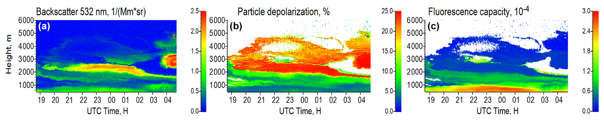
Figure 6 Spatiotemporal distributions of (a) the backscattering coefficient at 532 nm, (b) the particle depolarization ratio at 532 nm, and (c) the fluorescence capacity during the night of 1–2 October 2023. The depolarization ratio and fluorescence capacity are only calculated for values of β₅₃₂ > 0.1 Mm⁻¹ sr⁻¹.

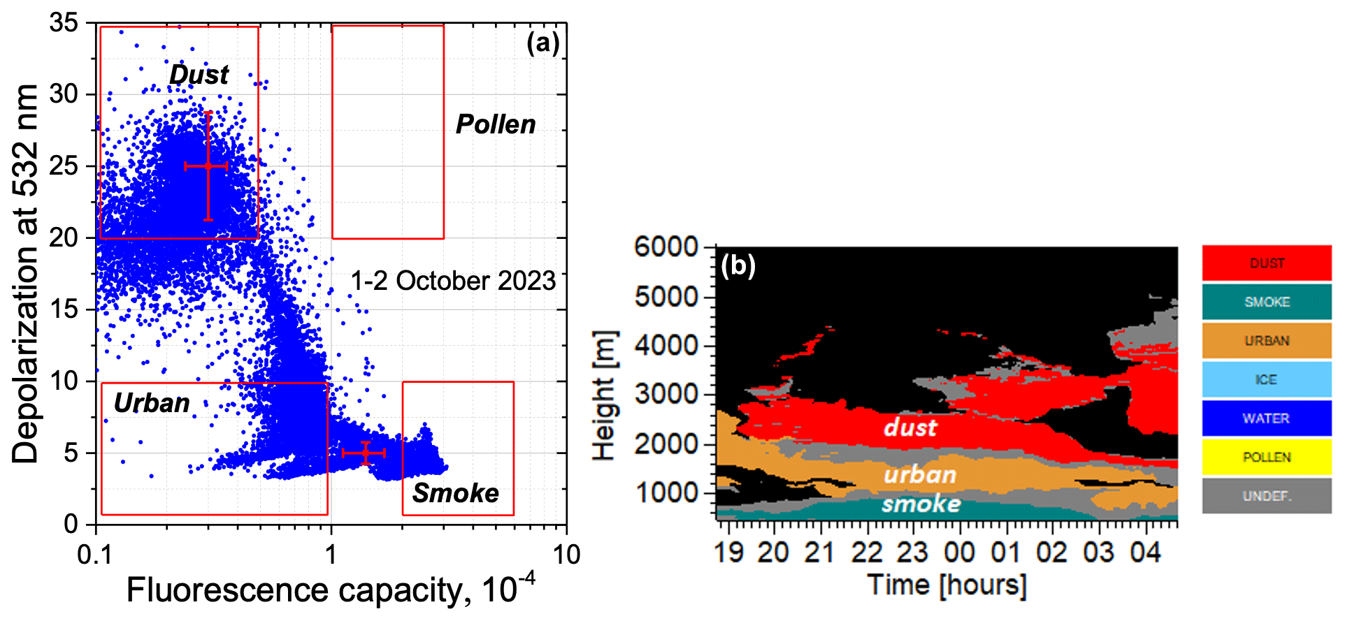
Figure 7 (a) The δ₅₃₂–G_F diagram and (b) the spatiotemporal distribution of aerosol types during the night of 1–2 October 2023.

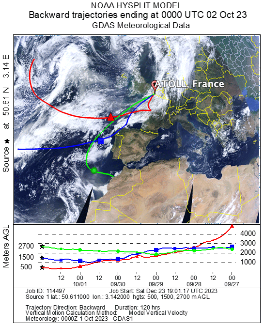
Figure 8 The HYSPLIT 5 d backward trajectories for the air mass over Lille at altitudes 500, 1500, and 2700 m on 2 October 2023 at 00:00 UTC.

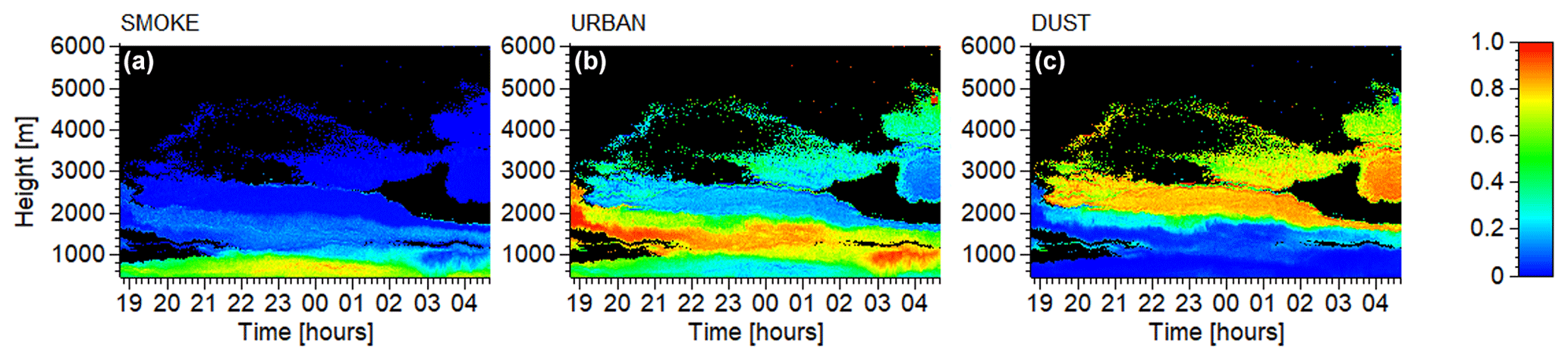
Figure 9 The relative contributions of (a) smoke (η_s), (b) urban (η_u), and (c) dust (η_d) particles to the backscattering coefficient β₅₃₂ during the night of 1–2 October 2023.

Figure 10 Vertical profiles of the relative contributions of smoke (η_s), urban (η_u), and dust (η_d) particles to the backscattering coefficient β₅₃₂ on 1 October 2023. The profiles are derived under the assumption that only three aerosol types occur. The black lines depict the deviation of solutions from the mean value (η_i ± σ_i). The magenta lines show the relative contributions of smoke, dust and urban particles (η_s,4, η_u,4, η_d,4) when four aerosol types (including pollen) are considered.

Table 2 Lidar ratios ($S_{\mathrm{532}}^i$) and extinction-to-volume conversion factors ($C_{\mathrm{V}}^i$) for different types of aerosol.

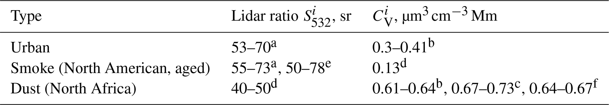
^a Burton et al. (2013). ^b Mamouri and Ansmann (2017). ^c Ansmann et al. (2019). ^d Ansmann et al. (2021). ^e Hu et al. (2022). ^f He et al. (2023).

3.4 Heat wave over Lille in July 2022

The heat wave in France in July 2022 was attributed to a high-pressure system known as the Azores High, which usually sits off Spain but pushed farther north, resulting in elevated temperatures and multiple fires. The Sun photometer and lidar observations at ATOLL consistently recorded an increase in aerosol content over Lille in the middle of July 2022. Figure 11 displays the aerosol optical depth (AOD) at 500 nm and the Ångström exponent for 380–500 nm wavelengths provided by AERONET. Lidar observations were performed from 16 to 23 July, as shown in the frame in Fig. 11. Within this interval, the optical depth increased, reaching its peak on 18 July. The Ångström exponent decreased, indicating the presence of dust. Figure 12 shows the column-integrated particle volume, provided by AERONET, presented separately for the fine- and coarse-mode particles. After 16 July, the volume of the coarse mode increased approximately 4-fold, while the fine mode did not show significant changes, further supporting the presence of dust particles. Unfortunately, volume retrievals are not available after 20 July due to the presence of clouds. The methodology outlined in Sect. 2.2 was used to analyze the composition of aerosols during the heat wave.

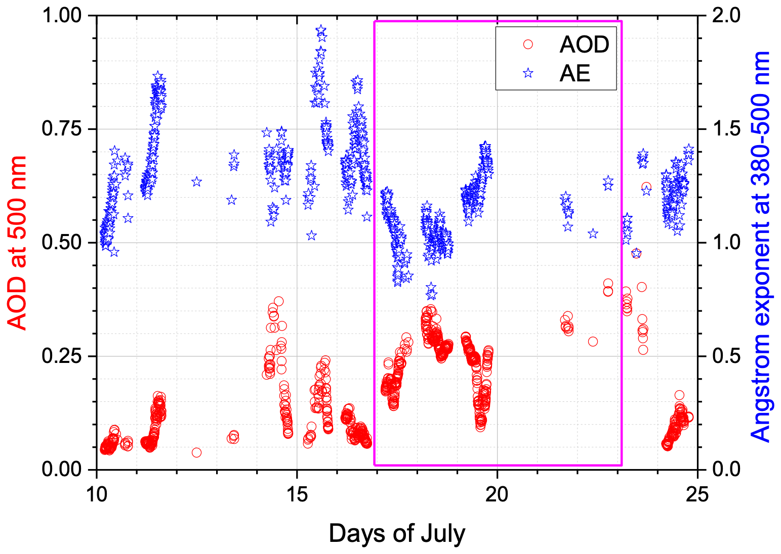
Figure 11 The aerosol optical depth (AOD) at 500 nm and the Ångström exponent (AE) provided by AERONET over Lille in July 2022. Magenta box depicts the time period during which lidar observations in this study were analyzed.

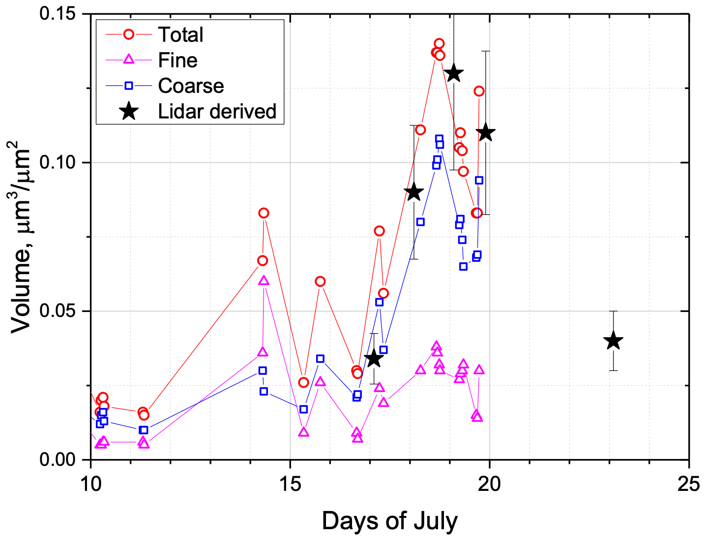
Figure 12 Column-integrated aerosol volume (circles) in July 2022 provided by AERONET. The triangles and squares represent the volumes of the fine and coarse modes, respectively. Black stars depict the total particle volume derived from lidar observations.

In Fig. 13, we can see the spatiotemporal distributions of β₅₃₂, δ₅₃₂, and G_F for four measurement sessions between 16 and 23 July 2022. On 16–17 July, after midnight, a dust layer with δ₅₃₂ exceeding 20 % appeared at a height of 5 km. The following night (17–18 July), the lower border of the dust layer descended to 2 km. By the night of 18–19 July, we observed strong aerosol backscattering (above 1.0 Mm⁻¹ sr⁻¹) from the ground up to a height of 5 km. Dust was primarily found within two height ranges: 0.75–2.0 and 3.0–5.0 km, where the particle depolarization ratio δ₅₃₂ exceeded 20 %. The aerosol between these dust layers showed high fluorescence capacity (above $\mathrm{2.0}\times {\mathrm{10}}^{-\mathrm{4}}$), indicating the presence of smoke. Unfortunately, we could not make long-term lidar observations from 19–21 July due to cloud cover. However, by the night of 22–23 July, we observed localized aerosols below 3 km. The values of δ₅₃₂ and G_F were below 10 % and $\mathrm{1.0}\times {\mathrm{10}}^{-\mathrm{4}}$, respectively, which is typical of urban particles. The relative humidity during the measurements for 16–19 July was below 60 % within the height range being considered. On the night of 22–23 July, the relative humidity was higher, reaching up to 80 %. In Fig. 14, we provide the G_F–δ₅₃₂ diagrams for the measurements shown in Fig. 13. On the night of 16–17 July, the clusters corresponding to dust and smoke and urban particles are distinct. However, for 17–19 July, dust was mixed with smoke and urban particles, resulting in a characteristic pattern on the G_F–δ₅₃₂ diagram (Veselovskii et al., 2022). By the night of 22–23 July, only one cluster, corresponding to urban aerosol, was observed. The distributions of particle types in Fig. 14 for the period of 16–19 July contain extended grey regions where different types of particles are mixed and cannot be identified. In Fig. 15, we can see the partition technique used to evaluate the contributions of dust, smoke, and urban aerosol to β₅₃₂. From this analysis, we can conclude that on the night of 16–17 July, the aerosol below 2.5 km was a mixture of smoke and urban particles, and the elevated dust layer (00:00–03:00 UTC) contained a significant amount of urban particles (η_u is up to 0.4). On 18–19 July, the aerosol between the two dust layers, within the height range of 2–3 km, was also a mixture of smoke and urban particles.

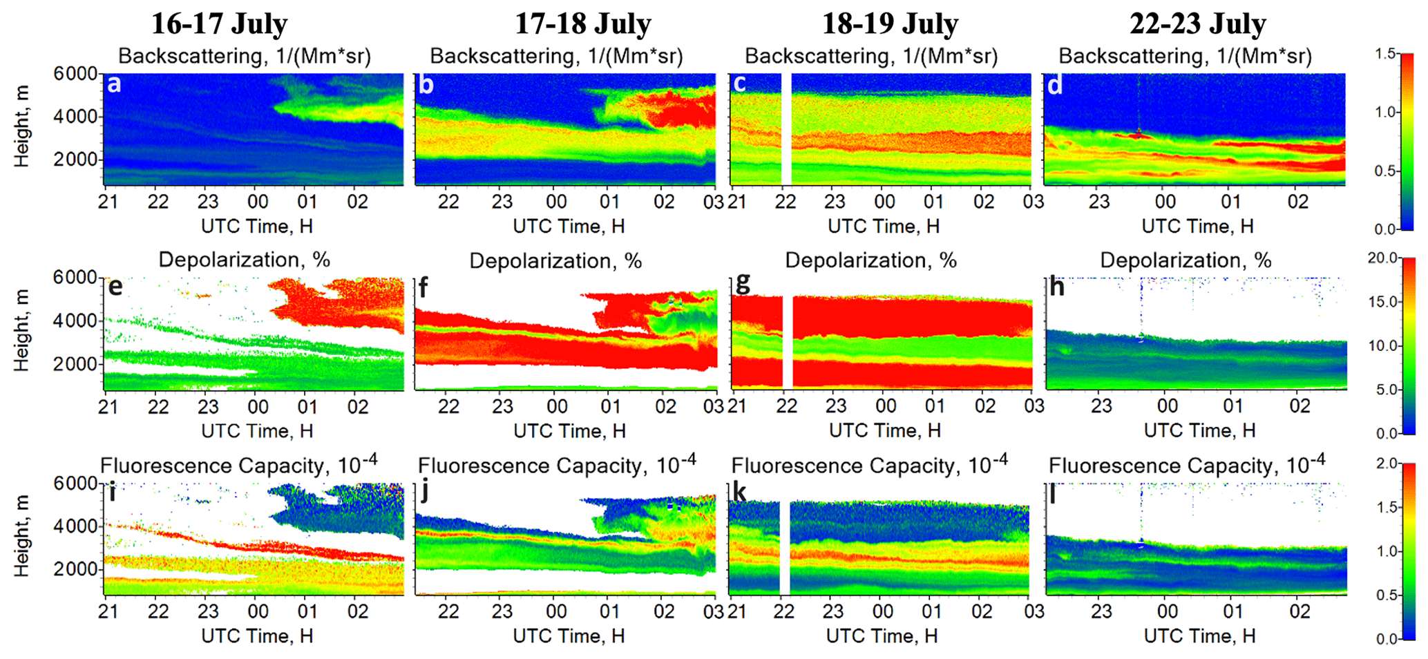
Figure 13 Spatiotemporal distributions of (a–d) the backscattering coefficient β₅₃₂, (e–h) the particle depolarization ratio δ₅₃₂, and (i–l) the fluorescence capacity G_F for the nights of 16–17, 17–18, 18–19, and 22–23 July 2022. The depolarization ratio and fluorescence capacity are only calculated for the values β₅₃₂ > 0.1 Mm⁻¹ sr⁻¹.

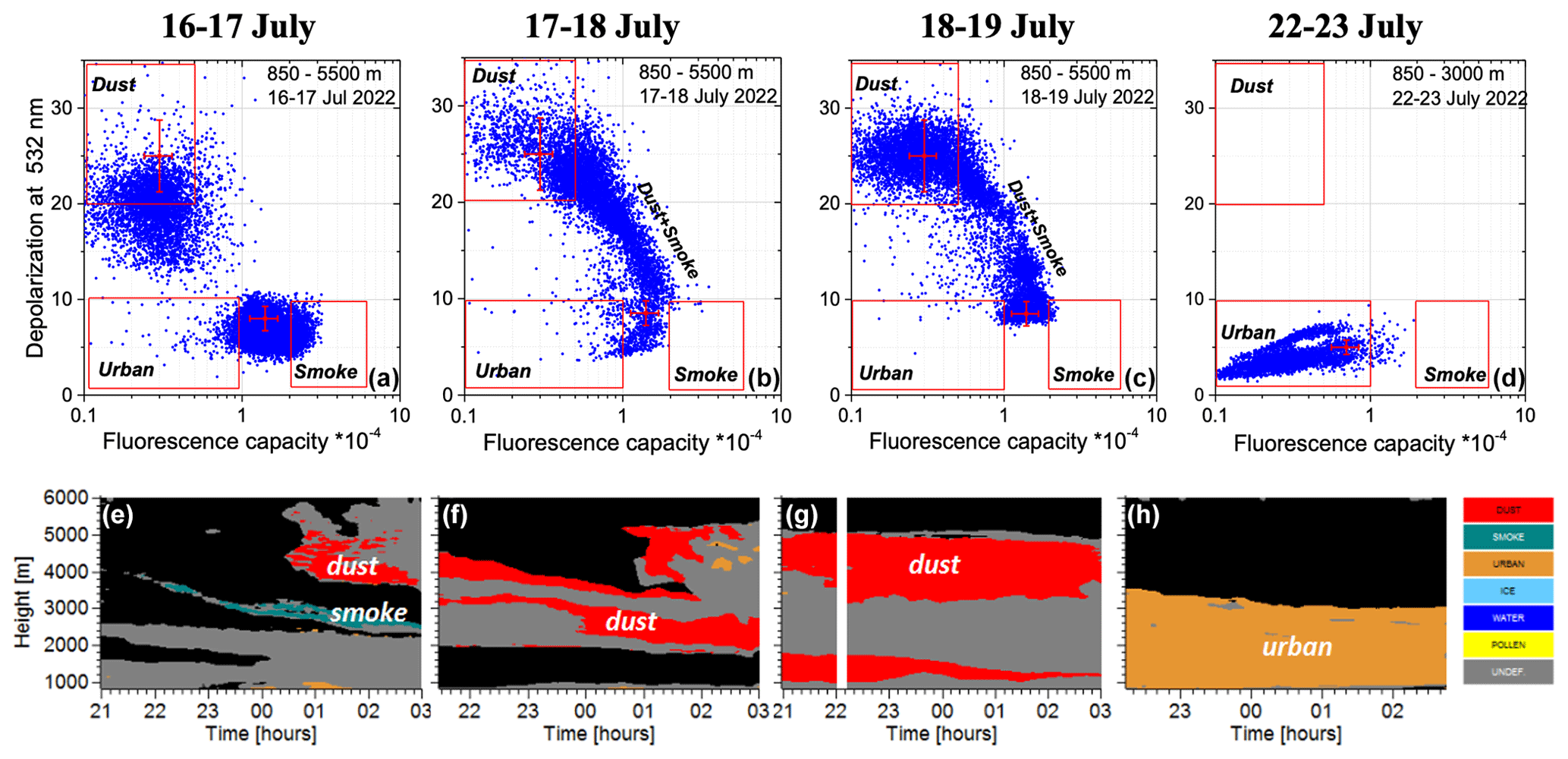
Figure 14 (a–d) The δ₅₃₂–G_F diagram and (e–h) the spatiotemporal distribution of aerosol types for the nights of 16–17, 17–18, 18–19, and 22–23 July 2022. The grey coloring represents an undefined aerosol type.

The aerosol classification based on fluorescence and depolarization measurements is supported by the analysis of backward trajectories. Figure 16 shows the 5 d backward trajectories for four measurement sessions from Fig. 15 at altitudes of 1500, 3000, and 4500 m. On 16–17 July, the dust layer above 4000 m originates from North Africa, while smoke at 3000 m is likely transported from North America. The air masses at 3000 m on 17–18 July are transported from Africa over regions of wildfires in Spain, indicating a mixture of dust and smoke. Smoke at 3000 m on 18–19 July again originates from wildfires in Spain, while the source of the dust layers at 1500 and 4000 m is in Africa. Finally, on 22–23 July, the heat wave was over. The air masses arrive from the west outside dust and smoke sources, and aerosol in Fig. 15 within the 1000–3000 m range is identified as urban.

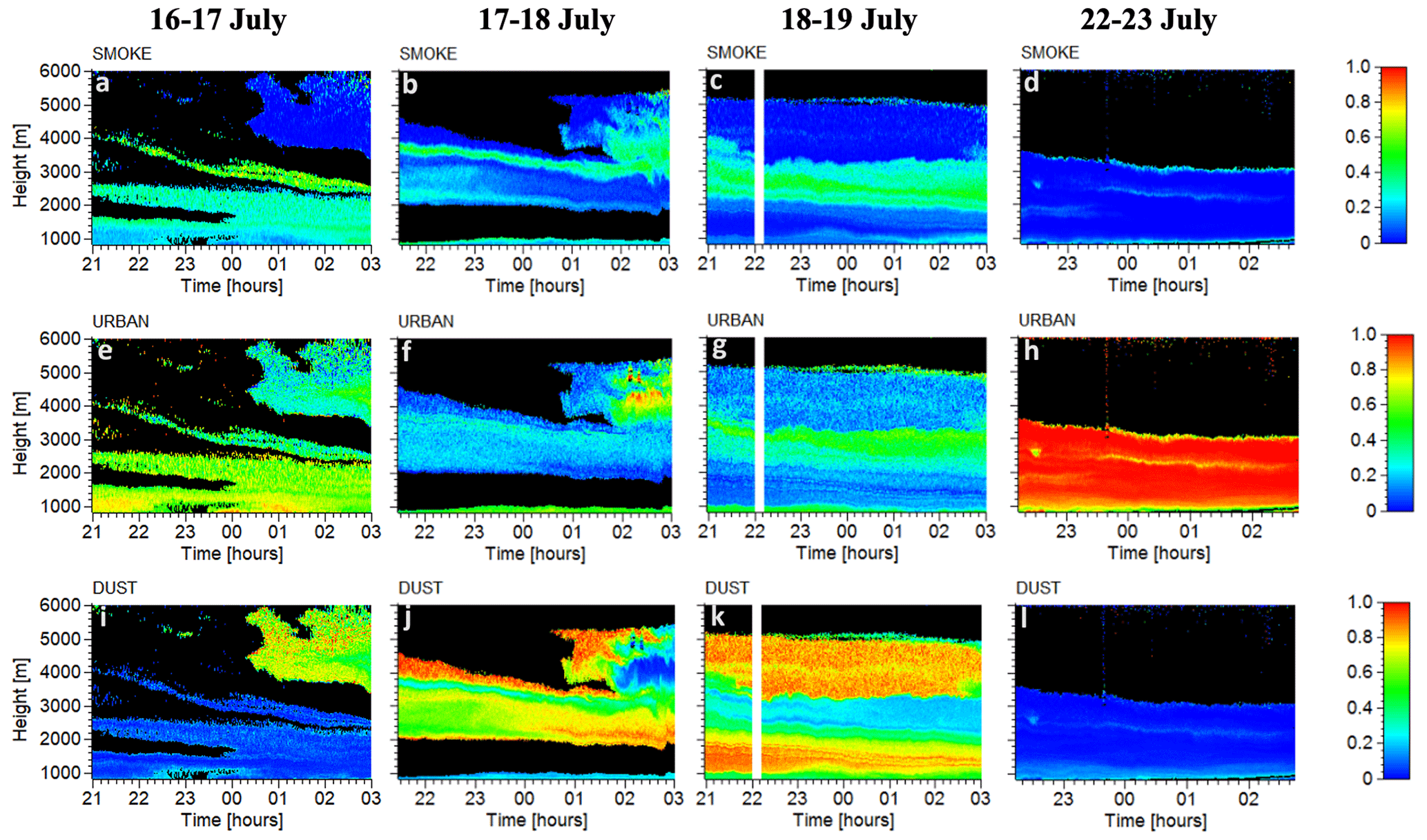
Figure 15 The relative contributions of (a–d) smoke, (e–h) urban, and (i–l) dust particles to the backscattering coefficient at 532 nm for the nights of 16–17, 17–18, 18–19, and 22–23 July 2022.

Figure 16 The HYSPLIT 5 d backward trajectories for the air mass over Lille at altitudes of 1500, 3000, and 4500 m on (a) 17 July 2022 at 03:00 UTC, (b) 17 July 2022 at 23:00 UTC, (c) 18 July 2022 at 22:00 UTC, and (d) 22 July 2022 at 22:00 UTC. Red dots depict the regions of forest fires.

As mentioned, the volume concentration of each component can be estimated using Eq. (8). Figure 17 presents the vertical profiles of volume concentration for smoke, urban, and dust particles for four measurement sessions from Fig. 15. In the calculations, we used the mean values of η_s, η_u, and η_d as well as the mean values of the lidar ratios and fluorescence capacity from Table 2. The lidar ratios used for smoke, urban, and dust are 64, 61, and 45 sr, respectively, and extinction-to-volume conversion factors are 0.13, 0.35, and 0.7 µm³ cm⁻³ Mm. The main contributors to the volume are urban and dust particles, with smoke contributing noticeably only on 18 and 19 July, but with a volume density still below 5 µm³ cm⁻³. The volume concentration can be recalculated to the mass concentration if the particle density is known. The profiles of mass concentration are shown in Fig. 17 as dashed lines. In computations we utilized a smoke density of ρ_s = 1.15 g cm⁻³ (Ansmann et al., 2021) and a dust density of ρ_d = 2.6 g cm⁻³ (He et al., 2023). For urban aerosol, a density of ρ_u = 1.5 g cm⁻³ was selected for sulfate particles.

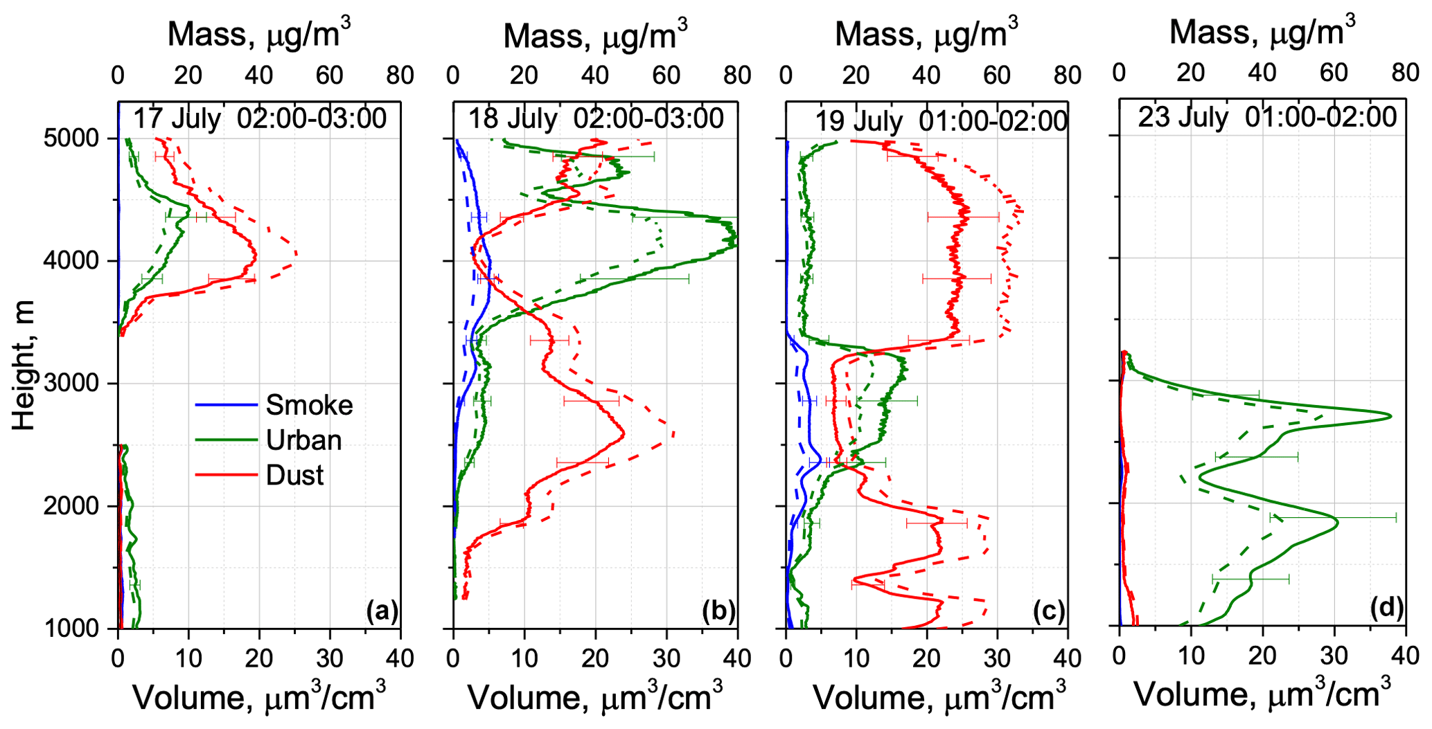
Figure 17 Vertical profiles of the volume concentration of smoke, dust, and urban particles derived from η_s, η_u, and η_d presented in Fig. 15, using the mean values of the lidar ratios and the conversion factors from Table 2. Profiles are shown for the episodes on (a) 17 July, (b) 18 July, (c) 19 July, and (d) 23 July 2022. Dashed lines depict the mass concentration calculated for the particle densities ρ_s = 1.15 g cm⁻³, ρ_u = 1.5 g cm⁻³, and ρ_d = 2.6 g cm⁻³.

To assess the validity of our volume estimations, we compared our results with AERONET retrievals. For this comparison, the volume density profiles of each component from Fig. 17 were extrapolated to the ground, and the total column-integrated volume was calculated. The results are depicted in Fig. 12 by stars, with an additional measurement on 19 July (22:00–23:00) included. It is evident that the results provided by AERONET are in reasonable agreement with the results provided by the lidar.

4 Conclusion

In conclusion, this study introduces an approach to partition aerosol mixtures in terms of backscattering coefficients, based on fluorescence and polarization lidar measurements. Specifically, we used the particle depolarization ratio at 532 nm and the fluorescence capacity, allowing for the partitioning of a three-component aerosol mixture at every height–time pixel. The robustness of this approach is demonstrated through testing with Mie–Raman–fluorescence lidar observations at the ATOLL instrumental site, providing valuable insights into the composition and dynamics of atmospheric aerosols. One notable advantage of the proposed approach is its applicability even in conditions of low aerosol content or for aerosol layers in the upper troposphere, where deriving profiles of extinction coefficients might be challenging. Additionally, backscattering coefficients of aerosol components can be converted to particle volume densities using corresponding lidar ratios along with extinction-to-volume conversion factors. While this conversion provides a rough volume estimation, considering the variability of the lidar ratios and the conversion factors within a given aerosol type, a comparison of lidar-derived particle volume during the heat wave over Lille in July 2022 demonstrates promising agreement with AERONET retrievals. At this stage, we have simplified our classification scheme by incorporating four aerosol types: smoke, dust, pollen, and urban particles. It is important to note that the use of fluorescence is an efficient way to distinguish between urban and smoke particles, which is a challenge for other methods that do not utilize fluorescence. However, we recognize the need to expand our approach to include additional aerosol types, particularly those with strong absorption such as polluted urban aerosol. This expansion will involve incorporating additional particle parameters, like lidar ratios, and is planned for our future research. It is crucial to acknowledge that the particle hygroscopic growth complicates the use of fluorescence capacity, resulting in increased uncertainty. To address this, we aim to utilize the additional independent information about aerosol type provided by the fluorescence spectrum. Importantly, the fluorescence spectrum is not affected by relative humidity. In our future research, we plan to further enhance the fluorescence capabilities by increasing the number of fluorescence channels in the lidar.