Variance estimations in the presence of intermittent interference and their applications to incoherent scatter radar signal processing

We discuss robust estimations for the variance of normally distributed random variables in the presence of interference. The robust estimators are based on either ranking or the geometric mean. For the interference models used, estimators based on the geometric mean outperform the rank-based ones in both mitigating the effect of interference and reducing the statistical error when there is no interference. One reason for this is that estimators using the geometric mean do not suffer from the “heavy tail” phenomenon like the rank-based estimators do. The ratio of the standard deviation over the mean of the power random variable is sensitive to interference. It can thus be used as a criterion to combine the sample mean with a robust estimator to form a hybrid estimator. We apply the estimators to the Arecibo incoherent scatter radar signals to determine the total power and Doppler velocities in the ionospheric E-region altitudes. Although all the robust estimators selected deal with light contamination well, the hybrid estimator is most effective in all circumstances. It performs well in suppressing heavy contamination and is as efficient as the sample mean in reducing the statistical error. Accurate incoherent scatter radar measurements, especially at nighttime and at E-region altitudes, can improve studies of ionospheric dynamics and composition.

1 Introduction

In radar signal processing and in many other applications, the data samples can often be modeled as a constant superimposed on a normally distributed random variable. The variance of the random process is an important parameter in such applications. In some cases, the variance represents the power of the undesired noise. In other cases, the variance is the desired signal power, such as in our study here on incoherent scatter radar (ISR) signals. Our broad objective is to explore methods that estimate the variance in a normally distributed random variable accurately in the presence of interference. The general problem falls under robust statistics (e.g., Huber and Ronchetti, 2009; Wilcox, 2017). Specifically, we attempt to optimize ISR signal processing using robust estimators.

An ISR, with a large aperture and high transmitting power, measures the electron concentration and other state variables in the ionosphere. Its versatility makes it the most important ground-based instrument for ionospheric studies. Several major ISRs started operation in the 1960s. Readers are referred to Evans (1969) for the principle, capabilities, and comparisons of the early facilities. An ISR typically transmits a binary-phase code to increase the signal-to-noise ratio. The received signal consists of sequences of altitude-dependent in-phase and quadrature voltage samples, which, upon decoding, can be used to obtain a variety of ionosphere parameters such as electron density and electron and ion temperatures (e.g., Zhou et al., 1997; Isham et al., 2000; Hysell et al., 2014). An essential characteristic of the voltage samples is that they are normally distributed, with the variance proportional to the electron density at the corresponding altitude. Because an ISR measures the tiny amount of power scattered off the electrons and ions in space, averaging over 1000 samples is essential to derive ionospheric parameters. In the absence of interference, a simple arithmetic average of the voltage samples squared provides the best estimator for the total power or power spectral density estimates, which form the foundation for the derivation of various ionospheric and atmospheric variables. It is well known, however, that the sample mean is susceptible to outliers. In many cases, it is necessary to use other estimators to obtain meaningful averages.

The ISR signal is subject to both active and passive interference. The former can be from other radars and TV stations. The latter can be from scattering off ships, satellites, and other objects. The most significant interference source for ISRs is micro-meteors, although they are the desired signal in the context of meteor studies (e.g., Zhou et al., 1995; Chau et al., 2007; Li et al., 2023). Meteor echoes come in diverse strengths and durations and provide the physical basis for constructing the interference model in our simulations. The incoherent scatter radar signal provides a textbook case for a normally distributed random variable that exists in nature. The high sensitivity of an ISR makes it susceptible to various types of interference. ISR signals thus provide a good test bed to evaluate the performance of various estimators.

In the following section, we discuss the statical characteristics of various estimators and compare their performance through theoretical analysis and numerical simulations for different interference scenarios. The aim here is to find an estimator that performs well with and without interference. In Sect. 3, we compare the performance of several estimators for total ISR power and Doppler velocity processing. We show that the hybrid estimator performs best for practically all the interference scenarios, and it is essentially as effective as the sample mean in reducing the statistical error.

2 Characteristics and comparison of mean power estimators

2.1 Signal and interference models

Let X be an independent identically distributed normal random variable having N=N₁N₂ data samples organized as

$${\displaystyle }X=\left\{\begin{array}{ccc}{x}_{\mathrm{11}}& \mathrm{\cdots }& x_{\mathrm{1}{N}_{\mathrm{1}}}\\ \mathrm{⋮}& \mathrm{\ddots }& \mathrm{⋮}\\ x_{N_{\mathrm{2}}\mathrm{1}}& \mathrm{\cdots }& x_{N_{\mathrm{2}}{N}_{\mathrm{1}}}\end{array}\right\}.$$

For radar and many other digital sampling systems, $X\sim N(\mathrm{0},{\mathit{\sigma }}^{\mathrm{2}})$ can be regarded as voltage samples. $Y=\mathit{\{}\frac{\mathrm{1}}{N_{\mathrm{1}}}{\sum }_{n_{\mathrm{1}}=\mathrm{1}}^{N_{\mathrm{1}}}{x}_{\mathrm{1}{n}_{\mathrm{1}}}^{\mathrm{2}},\frac{\mathrm{1}}{N_{\mathrm{1}}}{\sum }_{n_{\mathrm{1}}=\mathrm{1}}^{N_{\mathrm{1}}}{x}_{\mathrm{2}{n}_{\mathrm{1}}}^{\mathrm{2}},\mathrm{\dots },\frac{\mathrm{1}}{N_{\mathrm{1}}}{\sum }_{n_{\mathrm{1}}=\mathrm{1}}^{N_{\mathrm{1}}}{x}_{N_{\mathrm{2}}{n}_{\mathrm{1}}}^{\mathrm{2}}\mathit{\}}$ represents the power random variable with N₂ elements. Each element in Y is a sample mean of N₁ raw power variables, X². The expectation of Y_i is ${\mathit{\sigma }}_{\mathrm{0}}^{\mathrm{2}}$, which is the variance of X. We strive to estimate ${\mathit{\sigma }}_{\mathrm{0}}^{\mathrm{2}}$ most accurately, given samples of X. As there are many types of variances, we will call estimating ${\mathit{\sigma }}_{\mathrm{0}}^{\mathrm{2}}$ “power estimation” to be specific and to minimize confusion. In the absence of interference, Y_i can be shown to have a gamma probability density distribution (pdf):

$$\begin{array}{}\text{(1)}& f\left(y;{\displaystyle \frac{N_{\mathrm{1}}}{\mathrm{2}}},{\displaystyle \frac{\mathrm{2}{\mathit{\sigma }}_{\mathrm{0}}^{\mathrm{2}}}{N_{\mathrm{1}}}}\right)={\displaystyle \frac{y^{\frac{N_{\mathrm{1}}}{\mathrm{2}}-\mathrm{1}}{e}^{-\frac{y{N}_{\mathrm{1}}}{\mathrm{2}{\mathit{\sigma }}_{\mathrm{0}}^{\mathrm{2}}}}}{\mathrm{\Gamma }\left(\frac{N_{\mathrm{1}}}{\mathrm{2}}\right)}}{\left({\displaystyle \frac{N_{\mathrm{1}}}{\mathrm{2}{\mathit{\sigma }}_{\mathrm{0}}^{\mathrm{2}}}}\right)}^{\frac{N_{\mathrm{1}}}{\mathrm{2}}},\end{array}$$

where $\frac{N_{\mathrm{1}}}{\mathrm{2}}$ and $\frac{\mathrm{2}{\mathit{\sigma }}_{\mathrm{0}}^{\mathrm{2}}}{N_{\mathrm{1}}}$ are the shape and scale parameters, respectively, and the support of y is (0,∞) (e.g., Wikipedia, 2024b). The corresponding cumulative distribution function is

$$\begin{array}{}\text{(2)}& {\displaystyle }\begin{array}{rl}{\displaystyle }F\left(y;{\displaystyle \frac{N_{\mathrm{1}}}{\mathrm{2}}},{\displaystyle \frac{\mathrm{2}{\mathit{\sigma }}_{\mathrm{0}}^{\mathrm{2}}}{N_{\mathrm{1}}}}\right)& {\displaystyle }={\displaystyle \frac{\mathrm{1}}{\mathrm{\Gamma }\left(\frac{N_{\mathrm{1}}}{\mathrm{2}}\right)}}\mathit{\gamma }\left({\displaystyle \frac{N_{\mathrm{1}}}{\mathrm{2}}},{\displaystyle \frac{N_{\mathrm{1}}}{\mathrm{2}{\mathit{\sigma }}_{\mathrm{0}}^{\mathrm{2}}}}y\right)\\ {\displaystyle }& {\displaystyle }={\displaystyle \frac{\mathrm{1}}{\mathrm{\Gamma }\left(\frac{N_{\mathrm{1}}}{\mathrm{2}}\right)}}{\int }_{\mathrm{0}}^{\frac{N_{\mathrm{1}}}{\mathrm{2}{\mathit{\sigma }}^{\mathrm{2}}}y}{t}^{\frac{N_{\mathrm{1}}}{\mathrm{2}}-\mathrm{1}}{e}^{-t}\mathrm{d}t,\end{array}\end{array}$$

where $\mathit{\gamma }(s,x)={\int }_{\mathrm{0}}^x{t}^{s-\mathrm{1}}{e}^{-t}\mathrm{d}t$ is the lower incomplete gamma function. Distribution function f(y) can also be viewed as a N₁-degree chi-squared distribution scaled by N₁. The variance of Y_i is $\frac{\mathrm{2}{\mathit{\sigma }}_{\mathrm{0}}^{\mathrm{4}}}{N_{\mathrm{1}}}$. The distribution functions at N₁=1, 2, and 8, which we will study in more detail, are $f(y;\frac{\mathrm{1}}{\mathrm{2}},\mathrm{2}{\mathit{\sigma }}_{\mathrm{0}}^{\mathrm{2}})=\frac{e^{-\frac{y}{\mathrm{2}{\mathit{\sigma }}_{\mathrm{0}}^{\mathrm{2}}}}}{\sqrt{\mathrm{2}\mathit{\pi }y}{\mathit{\sigma }}_{\mathrm{0}}}$, $f(y;\mathrm{1},{\mathit{\sigma }}_{\mathrm{0}}^{\mathrm{2}})=\frac{e^{-\frac{y}{{\mathit{\sigma }}_{\mathrm{0}}^{\mathrm{2}}}}}{{\mathit{\sigma }}_{\mathrm{0}}^{\mathrm{2}}}$, and $f(y;\mathrm{4},\frac{{\mathit{\sigma }}_{\mathrm{0}}^{\mathrm{2}}}{\mathrm{4}})=\frac{{\mathrm{2}}^{\mathrm{7}}{y}^{\mathrm{3}}{e}^{-\frac{\mathrm{4}y}{{\mathit{\sigma }}_{\mathrm{0}}^{\mathrm{2}}}}}{\mathrm{3}{\mathit{\sigma }}_{\mathrm{0}}^{\mathrm{8}}}$, respectively. At large N₁, the pdf is approximately normal, $f(y;\frac{N_{\mathrm{1}}}{\mathrm{2}},\frac{\mathrm{2}{\mathit{\sigma }}_{\mathrm{0}}^{\mathrm{2}}}{N_{\mathrm{1}}})\sim N({\mathit{\sigma }}_{\mathrm{0}}^{\mathrm{2}},\frac{\mathrm{2}{\mathit{\sigma }}_{\mathrm{0}}^{\mathrm{4}}}{N_{\mathrm{1}}})$. Of particular interest is the case of N₁=2, which corresponds to the in-phase and quadrature samples in a radar system.

The interference is also modeled as a gamma distribution with a shape parameter of k=4 and scale parameter $(a_{\mathit{\eta }}{\mathit{\sigma }}_{\mathrm{0}}{)}^{\mathrm{2}}/k$, which has a mean of $a_{\mathit{\eta }}^{\mathrm{2}}{\mathit{\sigma }}_{\mathrm{0}}^{\mathrm{2}}$. Since we are mainly concerned with the signal shape parameter being $\mathrm{1}/\mathrm{2}$ and 1, a larger shape parameter in the interference model makes it easier to differentiate between interference and signal, as the interference is more concentrated around a higher mean value. The interference is equally likely to occur at each data point, with a probability of p_η=0.01, and is always additive to the signal. The total interference power relative to the signal power is thus $p_{\mathit{\eta }}{a}_{\mathit{\eta }}^{\mathrm{2}}$. We will mainly consider three cases of interference with a_η=2, 6, and 18 to represent low, moderate, and strong interference, respectively.

2.2 Estimators and their characteristics in the absence of interference

The most common estimators are the sample mean, geometric mean, and median. The sample mean of Y is the arithmetic average of N₂ samples, i.e., $A_N\equiv \frac{\mathrm{1}}{N_{\mathrm{2}}}{\sum }_{i=\mathrm{1}}^{N_{\mathrm{2}}}{Y}_i$, where Y_i is the sample mean of X² averaged over N₁ samples. With a known shape parameter, the sample mean is the uniformly minimum-variance unbiased estimator (UMVUE) and maximum likelihood estimator (e.g., Siegrist, 2022; Wikipedia, 2024a). The geometric mean, $G_N\equiv {\left({\prod }_{i=\mathrm{1}}^{N_{\mathrm{2}}}{Y}_i\right)}^{\mathrm{1}/N_{\mathrm{2}}}$, and median, $D_N\equiv \text{med}(Y_{\mathrm{1}},\mathrm{\dots }{Y}_{N_{\mathrm{2}}})$, are more resistant to outliers but not effective in reducing the statistical fluctuations. Although the three basic estimators are largely at the opposite ends of efficiency vs. robustness, they can serve as building blocks for other estimators. In the following, we discuss the three basic estimators and compare them with a weighted mean, a hybrid estimator, and two trimmed estimators.

The effectiveness of a power estimator, Z, in reducing the statistical fluctuation is measured by the normalized variance

$$\begin{array}{}\text{(3)}& R^{\mathrm{2}}\left(Z\right)\equiv {\displaystyle \frac{N{\mathit{\sigma }}_z^{\mathrm{2}}}{\mathrm{2}{\mathit{\mu }}_Z^{\mathrm{2}}}},\end{array}$$

where ${\mathit{\sigma }}_z^{\mathrm{2}}$ and μ_Z are the variance and mean of the power estimator while the absolute error is of importance in some cases as well. For the sample mean estimator, A_N, its distribution is expressed by Eq. (1) with N₁ replaced by N. E(A_n) is ${\mathit{\sigma }}_{\mathrm{0}}^{\mathrm{2}}$ and the variance is $\mathrm{2}{\mathit{\sigma }}_{\mathrm{0}}^{\mathrm{4}}/N$. The theoretical expectation of R²(A_n) is thus 1 for the sample mean, which is the lowest that one can obtain. The inverse of R²(Z) is the efficiency of the estimator. It is of interest to note that since N averages can be expressed as the weighted means of N₁ and N−N₁ samples, it follows that the convolution of two gamma distributions remains a gamma distribution. This convolution invariance property is also true of most commonly used distributions, including binomial, Poisson, normal, and chi-squared distributions. In general, if the distribution function of the sum or mean remains the same type for different numbers of samples, it is convolution invariant.

The median and its variance do not appear to have a closed form for N₁ and N₂ in general, although there are closed forms for specific N₁ and large N. Here we derive the theoretical results for N₁=1, 2, 8, and large N. For large N₂ and an ascending ranking order K relatively close to $N_{\mathrm{2}}/\mathrm{2}$, Zhou et al. (1999) show that ranking has an asymptotic normal distribution, with a variance of ${\mathit{\sigma }}_{N_{\mathrm{2}}K}^{\mathrm{2}}=\frac{K(N_{\mathrm{2}}-K)}{N_{\mathrm{2}}^{\mathrm{3}}{f}^{\mathrm{2}}\left({\mathit{\mu }}_{\mathrm{r}}\right)}$, where μ_r is the ranking value (e.g., $K=N_{\mathrm{2}}/\mathrm{2}$ for median) and f(μ_r) is the pdf for the rank random variable, i.e., Eq. (1) for our study here. For the median estimator, the normalized variance is

$$\begin{array}{}\text{(4)}& R^{\mathrm{2}}\left(D_N\right)={\displaystyle \frac{N_{\mathrm{1}}}{\mathrm{8}{f}^{\mathrm{2}}({\mathit{\mu }}_{\mathrm{r}};N_{\mathrm{1}}/\mathrm{2},\mathrm{2}/N_{\mathrm{1}}){\mathit{\mu }}_{\mathrm{r}}^{\mathrm{2}}}}.\end{array}$$

The median can be solved from $F\left({\mathit{\mu }}_{\mathrm{r}}\right)=\mathrm{1}/\mathrm{2}$. For N₁=1, the median is $\mathrm{2}{\text{ierf}}^{\mathrm{2}}\left(\frac{\mathrm{1}}{\mathrm{2}}\right){\mathit{\sigma }}_{\mathrm{0}}^{\mathrm{2}}=\mathrm{0.4549}{\mathit{\sigma }}_{\mathrm{0}}^{\mathrm{2}}$, where ierf is the inverse of the error function $\frac{\mathrm{2}}{\sqrt{\mathit{\pi }}}{\int }_{\mathrm{0}}^x{e}^{-t^{\mathrm{2}}}\mathrm{d}t$. For N₁=2, the median is ${\mathit{\mu }}_{\mathrm{r}}={\mathit{\sigma }}_{\mathrm{0}}^{\mathrm{2}}\ln \mathrm{2}=\mathrm{0.6931}{\mathit{\sigma }}_{\mathrm{0}}^{\mathrm{2}}$. The median for N₁=8 is $\mathrm{0.9180}{\mathit{\sigma }}_{\mathrm{0}}^{\mathrm{2}}$, which can be solved from $\mathit{\gamma }(\mathrm{4},\mathrm{4}{\mathit{\mu }}_{\mathrm{r}})=\mathrm{3}$. For large N₁, the pdf tends toward normal and the median tends toward ${\mathit{\sigma }}_{\mathrm{0}}^{\mathrm{2}}$. The R²(D_N) values for N₁=1, 2, 8, and 100 and N=10 000 are 2.7206, 2.0814, 1.6848, and 1.5760, respectively. In the limiting case of N₁ and N₂ tending toward infinity, $R^{\mathrm{2}}\left(D_N\right)=\mathit{\pi }/\mathrm{2}$, indicating that it takes $\mathit{\pi }/\mathrm{2}$ times the number of samples for the median operator to achieve the same error as the sample mean. Zhou et al. (1999) also show that taking the 79.7 % largest value gives the smallest R² at 1.5432. (in Zhou et al., 1999, $\mathit{\pi }/\mathrm{2}$ in Eqs. 24 and 26 should have been $\mathrm{2}/\mathit{\pi }$.)

Table 1 Monte Carlo simulations and theoretical values (in parenthesis) of the mean, R², and absolute error for eight estimators when there is no interference.

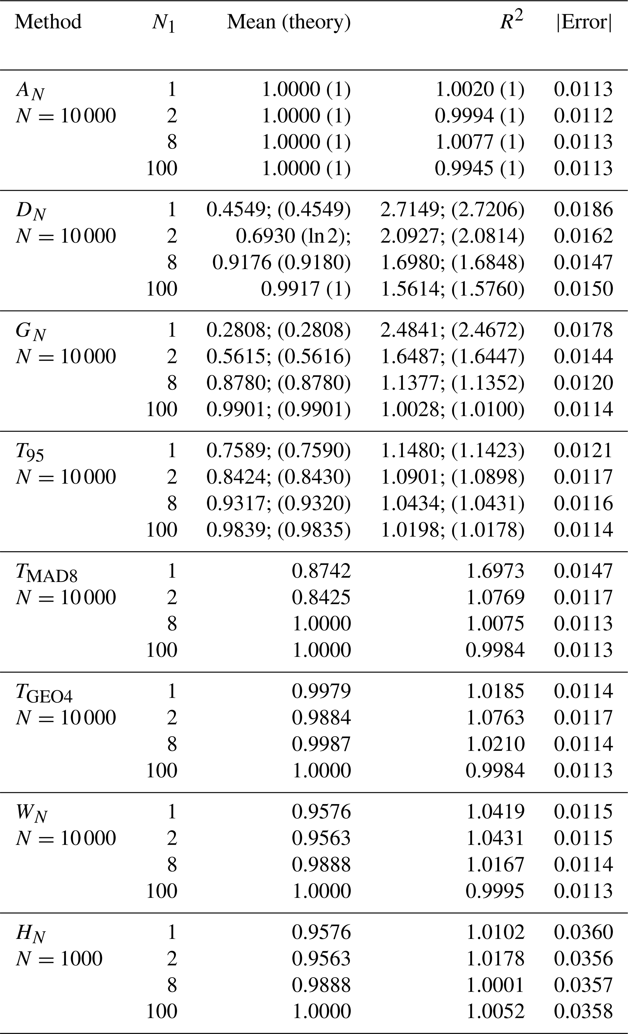
In Table 1, we list the R² values and the absolute errors for eight estimators in the null-interference case. The second column is the mean of each estimator without scaling for σ₀=1 (the mean is proportional to ${\mathit{\sigma }}_{\mathrm{0}}^{\mathrm{2}}$). To compare the different estimators on the same scale, the mean is divided by the respective estimator so that all the estimators in all the cases have a mean of 1 for all subsequent computations in the other columns in Tables 1 and 2. The values not in parentheses listed in the two tables are at least 100 000 Monte Carlo simulations with N=10 000 for all estimators except H_N. The values in parentheses in Table 1 are theoretical predictions that we can derive.

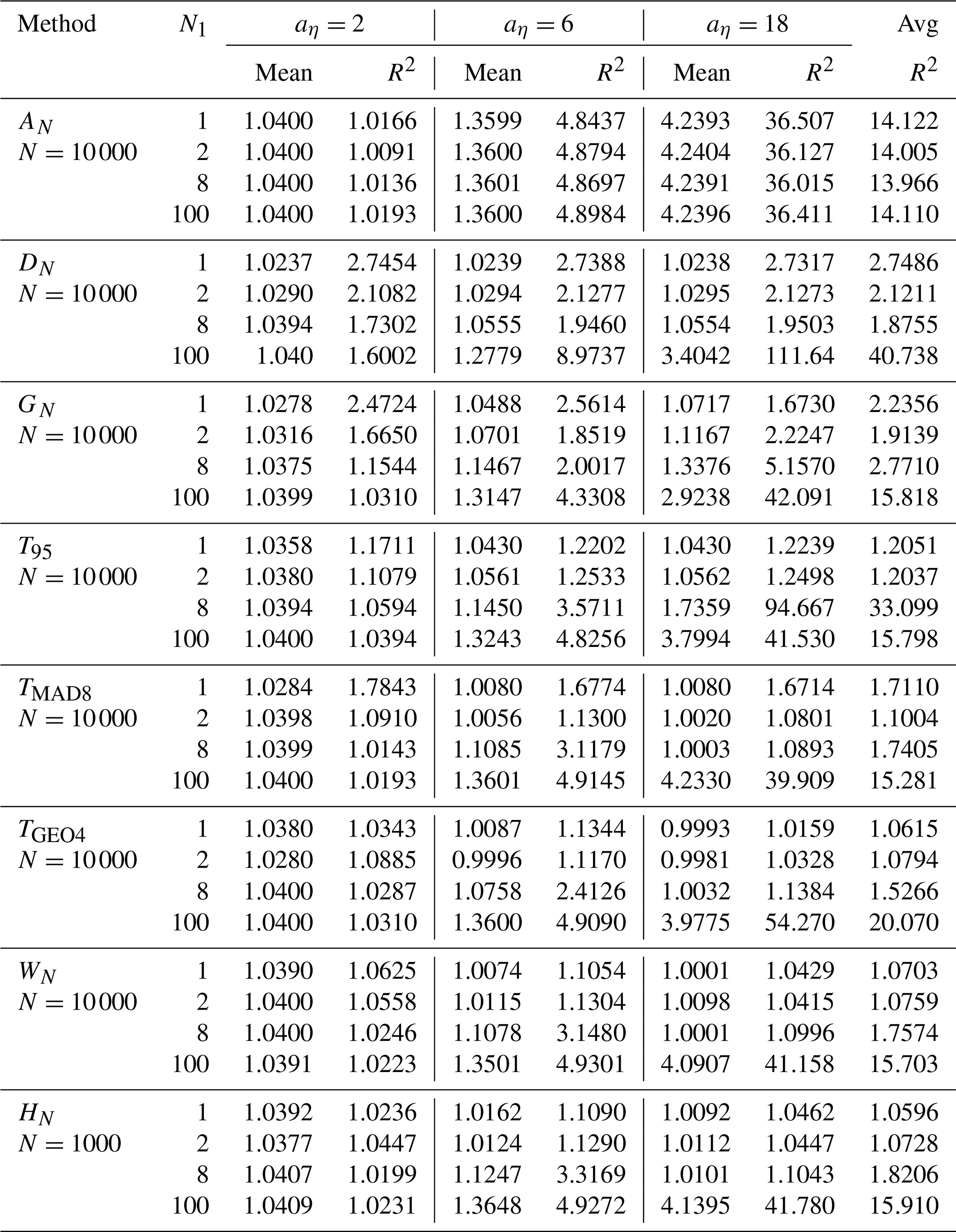
Table 2 Mean and R² values for low, moderate, and strong interference. The interference occurrence rate is p_η=0.01 for all three interference scenarios.

The mean and variance of the geometric mean (G_N) can be obtained by first finding the expectation and variance of one element, $Y_i^{\mathrm{1}//N_{\mathrm{2}}}$, in the product. The expectation of $Y_i^{\mathrm{1}//N_{\mathrm{2}}}$ is

$$\begin{array}{}\text{(5)}& E\left(y^{\frac{\mathrm{1}}{N_{\mathrm{2}}}}\right)=\underset{\mathrm{0}}{\overset{\mathrm{\infty }}{\int }}{y}^{\frac{\mathrm{1}}{N_{\mathrm{2}}}}f\left(y\right)\mathrm{d}y={\displaystyle \frac{\mathrm{\Gamma }(\frac{N_{\mathrm{1}}}{\mathrm{2}}+\frac{\mathrm{1}}{N_{\mathrm{2}}})}{\mathrm{\Gamma }\left(\frac{N_{\mathrm{1}}}{\mathrm{2}}\right)}}{\left({\displaystyle \frac{\mathrm{2}{\mathit{\sigma }}_{\mathrm{0}}^{\mathrm{2}}}{N_{\mathrm{1}}}}\right)}^{\frac{\mathrm{1}}{N_{\mathrm{2}}}}.\end{array}$$

The second moment of $Y_i^{\mathrm{1}/N_{\mathrm{2}}}$ is

$$\begin{array}{}\text{(6)}& E\left(y^{\frac{\mathrm{2}}{N_{\mathrm{2}}}}\right)=\underset{\mathrm{0}}{\overset{\mathrm{\infty }}{\int }}{y}^{\frac{\mathrm{2}}{N_{\mathrm{2}}}}f\left(y\right)\mathrm{d}y={\displaystyle \frac{\mathrm{\Gamma }(\frac{N_{\mathrm{1}}}{\mathrm{2}}+\frac{\mathrm{2}}{N_{\mathrm{2}}})}{\mathrm{\Gamma }\left(\frac{N_{\mathrm{1}}}{\mathrm{2}}\right)}}{\left({\displaystyle \frac{\mathrm{4}{\mathit{\sigma }}_{\mathrm{0}}^{\mathrm{4}}}{N_{\mathrm{1}}^{\mathrm{2}}}}\right)}^{\frac{\mathrm{1}}{N_{\mathrm{2}}}}.\end{array}$$

Assuming that Y_i's are independent, the expectation, second moment, and variance of the geometric mean are, respectively,

$$\begin{array}{}\text{(7)}& {\displaystyle }E\left(G_N\right)={\left(E\left(y^{\frac{\mathrm{1}}{N_{\mathrm{2}}}}\right)\right)}^{N_{\mathrm{2}}}={\displaystyle \frac{{\mathrm{\Gamma }}^{N_{\mathrm{2}}}(\frac{N_{\mathrm{1}}}{\mathrm{2}}+\frac{\mathrm{1}}{N_{\mathrm{2}}})}{{\mathrm{\Gamma }}^{N_{\mathrm{2}}}\left(\frac{N_{\mathrm{1}}}{\mathrm{2}}\right)}}{\displaystyle \frac{\mathrm{2}{\mathit{\sigma }}_{\mathrm{0}}^{\mathrm{2}}}{N_{\mathrm{1}}}},\text{(8)}& {\displaystyle }E\left(G_N^{\mathrm{2}}\right)={\left(E\left(y^{\frac{\mathrm{2}}{N_{\mathrm{2}}}}\right)\right)}^{N_{\mathrm{2}}}={\displaystyle \frac{{\mathrm{\Gamma }}^{N_{\mathrm{2}}}(\frac{N_{\mathrm{1}}}{\mathrm{2}}+\frac{\mathrm{2}}{N_{\mathrm{2}}})}{{\mathrm{\Gamma }}^{N_{\mathrm{2}}}\left(\frac{N_{\mathrm{1}}}{\mathrm{2}}\right)}}{\displaystyle \frac{\mathrm{4}{\mathit{\sigma }}_{\mathrm{0}}^{\mathrm{4}}}{N_{\mathrm{1}}^{\mathrm{2}}}},\text{(9)}& {\displaystyle }\text{Var}\left(G_N\right)={\displaystyle \frac{\mathrm{4}{\mathit{\sigma }}_{\mathrm{0}}^{\mathrm{4}}}{N_{\mathrm{1}}^{\mathrm{2}}}}\left({\displaystyle \frac{{\mathrm{\Gamma }}^{N_{\mathrm{2}}}(\frac{N_{\mathrm{1}}}{\mathrm{2}}+\frac{\mathrm{2}}{N_{\mathrm{2}}})}{{\mathrm{\Gamma }}^{N_{\mathrm{2}}}\left(\frac{N_{\mathrm{1}}}{\mathrm{2}}\right)}}-{\displaystyle \frac{{\mathrm{\Gamma }}^{\mathrm{2}{N}_{\mathrm{2}}}(\frac{N_{\mathrm{1}}}{\mathrm{2}}+\frac{\mathrm{1}}{N_{\mathrm{2}}})}{{\mathrm{\Gamma }}^{\mathrm{2}{N}_{\mathrm{2}}}\left(\frac{N_{\mathrm{1}}}{\mathrm{2}}\right)}}\right).\end{array}$$

The normalized variance for the geometric mean, R²(G_N), is thus

$$\begin{array}{}\text{(10)}& R^{\mathrm{2}}\left(G_N\right)={\displaystyle \frac{N_{\mathrm{1}}{N}_{\mathrm{2}}}{\mathrm{2}}}\left[{\left({\displaystyle \frac{\mathrm{\Gamma }\left(\frac{N_{\mathrm{1}}}{\mathrm{2}}\right)\mathrm{\Gamma }(\frac{N_{\mathrm{1}}}{\mathrm{2}}+\frac{\mathrm{2}}{N_{\mathrm{2}}})}{{\mathrm{\Gamma }}^{\mathrm{2}}(\frac{N_{\mathrm{1}}}{\mathrm{2}}+\frac{\mathrm{1}}{N_{\mathrm{2}}})}}\right)}^{N_{\mathrm{2}}}-\mathrm{1}\right].\end{array}$$

This equation is precise for all N₁ and N₂. E(G_N) and R²(G_N) values for N=10 000 and N₁=1, 2, 8, and 100 are listed in Table 1. We are not aware of a precise distribution function for G_N in general. For the asymptotic case of large N₂, Zhou et al. (1999) show that the geometric mean tends toward the normal distribution, with the variance as

$$\begin{array}{}\text{(11)}& \text{Var}\left(G_N\right){|}_{N_{\mathrm{2}}\to \mathrm{\infty }}={\displaystyle \frac{E^{\mathrm{2}}\left(G_N\right){\mathit{\sigma }}_{\text{ln}}^{\mathrm{2}}}{N_{\mathrm{2}}}},\end{array}$$

where ${\mathit{\sigma }}_{\text{ln}}^{\mathrm{2}}$ is the variance of ln (y). ${\mathit{\sigma }}_{\text{ln}}^{\mathrm{2}}$ is known to equal the trigamma function (${\mathit{\psi }}_{\mathrm{1}}\left(\frac{N_{\mathrm{1}}}{\mathrm{2}}\right)$; e.g., Wikipedia, 2024a). Thus,

$$\begin{array}{}\text{(12)}& R^{\mathrm{2}}\left(G_N\right){|}_{N_{\mathrm{2}}\to \mathrm{\infty }}={\displaystyle \frac{N_{\mathrm{1}}{\mathit{\sigma }}_{\text{ln}}^{\mathrm{2}}}{\mathrm{2}}}={\displaystyle \frac{N_{\mathrm{1}}}{\mathrm{2}}}{\mathit{\psi }}_{\mathrm{1}}\left({\displaystyle \frac{N_{\mathrm{1}}}{\mathrm{2}}}\right).\end{array}$$

For the trigamma function, ${\mathit{\psi }}_{\mathrm{1}}\left(\frac{\mathrm{1}}{\mathrm{2}}\right)=\frac{{\mathit{\pi }}^{\mathrm{2}}}{\mathrm{2}}$, ${\mathit{\psi }}_{\mathrm{1}}\left(\mathrm{1}\right)=\frac{{\mathit{\pi }}^{\mathrm{2}}}{\mathrm{6}}$, and other ${\mathit{\psi }}_{\mathrm{1}}\left(\frac{N_{\mathrm{1}}}{\mathrm{2}}\right)$ values can be found from the recurrence relation ${\mathit{\psi }}_{\mathrm{1}}(z+\mathrm{1})={\mathit{\psi }}_{\mathrm{1}}\left(z\right)-\mathrm{1}/z^{\mathrm{2}}$. The asymptotic R²(G_N) for $N_{\mathrm{1}}=[\mathrm{1},\mathrm{2},\mathrm{8},\mathrm{100}]$ and N=10 000 is $[\mathrm{2.4674},\mathrm{1.6449},\mathrm{1.3529},\mathrm{1.010}]$, respectively. They are accurate to the third decimal place compared to the exact values obtained from Eq. (10) for N₂=10 000. For large N₁ and N₂, $R^{\mathrm{2}}\left(G_N\right)\sim \mathrm{1}+\frac{\mathrm{1}}{N_{\mathrm{1}}}$, which gives the number of initial averages, N₁, needed to achieve a certain level of efficiency for the geometric mean. The expectation of G_N for large N₂ is found to be

$$\begin{array}{}\text{(13)}& {\displaystyle }\begin{array}{rl}{\displaystyle }E\left(G_N\right){|}_{N_{\mathrm{2}}\to \mathrm{\infty }}& {\displaystyle }\sim {\mathit{\sigma }}_{\mathrm{0}}^{\mathrm{2}}\left(\mathrm{1}+{\displaystyle \frac{\mathrm{2}}{N_{\mathrm{1}}{N}_{\mathrm{2}}}}\right)e^{-\frac{\mathrm{1}}{N_{\mathrm{1}}}-\frac{\mathrm{1}}{\mathrm{3}(N_{\mathrm{1}}+\mathrm{2}/N_{\mathrm{2}})N_{\mathrm{1}}}}\\ {\displaystyle }& {\displaystyle }\sim {\mathit{\sigma }}_{\mathrm{0}}^{\mathrm{2}}{e}^{-\frac{\mathrm{1}}{N_{\mathrm{1}}}-\frac{\mathrm{1}}{\mathrm{3}{N}_{\mathrm{1}}^{\mathrm{2}}}}\end{array}\end{array}$$

using the approximation $\ln \left(\mathrm{\Gamma }\right(z\left)\right)\sim z\ln \left(z\right)-z-\frac{\mathrm{1}}{\mathrm{2}}\ln \left(z\right)+\frac{\mathrm{1}}{\mathrm{12}z}+\frac{\mathrm{1}}{\mathrm{2}}\ln \left(\mathrm{2}\mathit{\pi }\right)$ (Wikipedia, 2024b). The variance of G_N at large N₂ is

$$\begin{array}{}\text{(14)}& {\displaystyle }\begin{array}{rl}{\displaystyle }\text{Var}\left(G_N\right){|}_{N_{\mathrm{2}}\to \mathrm{\infty }}& {\displaystyle }={\displaystyle \frac{E^{\mathrm{2}}\left(G_N\right){\mathit{\sigma }}_{\text{ln}}^{\mathrm{2}}}{N_{\mathrm{2}}}}\\ {\displaystyle }& {\displaystyle }={\displaystyle \frac{{\mathit{\psi }}_{\mathrm{1}}\left(\frac{N_{\mathrm{1}}}{\mathrm{2}}\right)}{N_{\mathrm{2}}}}{\mathit{\sigma }}_{\mathrm{0}}^{\mathrm{4}}{e}^{-\frac{\mathrm{2}}{N_{\mathrm{1}}}-\frac{\mathrm{2}}{\mathrm{3}{N}_{\mathrm{1}}^{\mathrm{2}}}}.\end{array}\end{array}$$

In Table 1, we list the theoretical values of the geometric mean and R² and their comparisons with the simulated values. We see that the theoretical values agree with simulations very well for all three basic estimators in the various scenarios.

As the median and other ranks are not efficient in reducing the statistical fluctuation, one can average the data within a certain percentile range, which is known as the trimmed or truncated mean. Since interference is additive, we will only be concerned with one-sided trimming below a fraction of β. Let b be the integer value of βN₂. The trimmed mean at β is $T_{\mathit{\beta }}\equiv \frac{\mathrm{1}}{b}{\sum }_{j=\mathrm{1}}^b\text{sort}(Y_i{)}_j$, where sort(Y_i) is Y_i sorted into ascending order. Let F(y_β)=β, ${\mathit{\mu }}_{\mathit{\beta }}=\frac{\mathrm{1}}{\mathit{\beta }}{\int }_{\mathrm{0}}^{y_{\mathit{\beta }}}yf\left(y\right)\mathrm{d}y$ and ${\mathit{\sigma }}_{\mathit{\beta }}^{\mathrm{2}}=\frac{\mathrm{1}}{\mathit{\beta }}{\int }_{\mathrm{0}}^{y_{\mathit{\beta }}}{y}^{\mathrm{2}}f\left(y\right)\mathrm{d}y-{\mathit{\mu }}_{\mathit{\beta }}^{\mathrm{2}}$. Stigler (1973) shows that the asymptotic mean and variance of T_β for large N₂ is E(T_β)=μ_β and ${\mathit{\sigma }}_T^{\mathrm{2}}=\frac{[\frac{{\mathit{\sigma }}_{\mathit{\beta }}^{\mathrm{2}}}{\mathit{\beta }}+\frac{\mathrm{1}-\mathit{\beta }}{\mathit{\beta }}{\left(y_{\mathit{\beta }}-{\mathit{\mu }}_{\mathit{\beta }}\right)}^{\mathrm{2}}]}{N_{\mathrm{2}}}$, respectively. The normalized variance for the trimmed mean is thus

$$\begin{array}{}\text{(15)}& R^{\mathrm{2}}\left(T_{\mathit{\beta }}\right)=N_{\mathrm{1}}{\displaystyle \frac{{\mathit{\sigma }}_{\mathit{\beta }}^{\mathrm{2}}+(\mathrm{1}-\mathit{\beta })(y_{\mathit{\beta }}-{\mathit{\mu }}_{\mathit{\beta }}{)}^{\mathrm{2}}}{\mathrm{2}\mathit{\beta }{\mathit{\mu }}_{\mathit{\beta }}^{\mathrm{2}}}}.\end{array}$$

In the following examples, N=10 000, β=0.95, and σ₀=1. If N₁=2, then y_β=3.843, μ_β=0.7590, ${\mathit{\sigma }}_{\mathit{\beta }}^{\mathrm{2}}=\mathrm{0.7747}$, and R²(T₉₅)=1.1423. If N₁=2, we have y_β=2.995, μ_β=0.8422, ${\mathit{\sigma }}_{\mathit{\beta }}^{\mathrm{2}}=\mathrm{0.5027}$, and R²(T₉₅)=1.0898. When N₁ is 8, then y_β=1.9384, μ_β=0.9320, ${\mathit{\sigma }}_{\mathit{\beta }}^{\mathrm{2}}=\mathrm{0.1645}$, and R²(T₉₅)=1.0431. For N₁=100, we have y_β=1.2435, μ_β=0.9835, ${\mathit{\sigma }}_{\mathit{\beta }}^{\mathrm{2}}=\mathrm{0.0153}$, and R²(T₉₅)=1.0178. As seen in Table 1, the R₂ values agree with the simulation very well. It is of interest to note that R₂ is not $\mathrm{1}/\mathrm{0.95}=\mathrm{1.05}$ as intuition might suggest. It varies from 1.142 at N₁=1 to 1.018 at N₁=100. When N₁=1, the tail is long and has more variations, leading to a large R² value – a tail-wagging-the-dog situation. More averaging makes the tail more stable and R² smaller. This phenomenon, and the effects of a “fat tail” or heavy tail, are extensively discussed by Resnick (2007) and Taleb (2022).

To estimate a parameter robustly, we can attempt to identify outliers and exclude them from the average. Most of the outlier classifying methods involve estimating a nominal deviation and using it in a threshold to detect outliers. The median absolute deviation (MAD), defined as $\text{MAD}=\text{med}\left(\right|Y_i-\text{med}\left(Y\right)\left|\right)$, is most frequently used to detect outliers (Huber and Ronchetti, 2009). Since only a small fraction of the ISR data is contaminated most of the time, we will classify a data point having 8 MADs above the median as an outlier. The sample mean of all non-outlier points is referred to as the T_MAD8 estimator. When there is no interference, R²(T_MAD8) is 1.6973, 1.0769, 1.0075, and 0.9984 for N₁=1, 2, 8, and 100, respectively. There is a significant improvement in R² from N₁=1 to N₁=8 because averaging reduces the number of spurious outliers significantly in the trimmed mean as discussed above. At N₁=1, the proportion of flagged outliers is about 0.2 %, while at N₁=8 the effective rate of flagged outliers is 0.0012 %. We note that Rousseeuw and Croux (1993) present two robust estimators that are more efficient than MAD, although more computationally intensive. With a normalized variance larger than 1.2, their estimators are better suited for heavy contamination.

As the geometric mean is resistant to outliers as well, it may also conceivably be used to classify outliers. We define the geometric deviation as ${\mathit{\sigma }}_G\equiv G_N{e}^{{\mathit{\sigma }}_{\text{ln}}\left(y\right)}-G_N$, where σ_log(y)=std(ln (y)). The dimensionless $e^{{\mathit{\sigma }}_{\text{log}}\left(y\right)}$ is known as the geometric standard deviation. σ_G is zero if all samples in Y are a constant and increase in proportion with Y, although ${\mathit{\sigma }}_G^{\mathrm{2}}$ does not have the usual properties of the variance as commonly defined. We average all the data points 4 geometric deviations below the geometric mean and refer to the estimator as T_GEO4. T_GEO4 and T_MAD8 are chosen to have almost the same normalized variance at N₁=2, as they flag out the same number of outliers in the absence of interference. When N₁=1, T_GEO4 has a far better R² value in the null-interference case.

Weighted means can also be used to mitigate the effect of outliers and interference. In this method, values far away from the expected mean are weighted less than those points around the mean. The weighting function we choose is $w_i=e^{-\frac{(y_i-m_{\text{G4}}{)}^{\mathrm{2}}}{\mathrm{40}{\mathit{\sigma }}_{\text{G4}}^{\mathrm{2}}}}$, where m_G4 and σ_G4 are the sample mean and standard deviation of the T_GEO4 estimator discussed above. The mean values of W_N for various N₁ are listed in Table 1. In the null-interference case, R²(W_N) is no larger than 1.046, or the efficiency is no less than 95.6 %. If the constant 40 is changed to 60, the worst R² becomes 1.031, but the weighted mean is less effective in mitigating the effect of outliers. The mean and standard deviation of T_GEO4 are chosen because of their general accuracy and computing efficiency.

Knowing whether interference exists can help mitigate its effect. For a gamma distribution, we cannot associate the existence of outliers with interference with certainty, as there are outliers even when there is no interference. Since the expectation of R² for the sample mean is known in the null-interference case, a deviation from the expectation indicates that the underlying process may contain interference. As the sample mean performs best when there is no interference, an expedient strategy to reduce the variance is to combine the sample mean when no interference is detected with another estimator that is effective in mitigating the interference. We have used N=10 000 for the asymptotic case for all the estimators discussed above. In combining different estimators, a smaller N value is preferred so that the combined estimator will not be dominated by the interference-mitigating estimator in the presence of interference. We can also define a mixed R² that uses the mean of the T_GEO4 estimator and the normally defined variance. Such a mixed R² is more sensitive to outliers, but its variance is larger. Simulations show it does not cause a material difference from R²(A_N) using the sample mean and standard deviation. Because of its simplicity, we choose R²(A_N) as the criterion to determine if the data samples follow the desired process. The decision rule for this hybrid estimator, H_N, is that if R(A_N) is less than 2 standard deviations above the mean, it uses the sample mean, otherwise the weighted mean is used. The performance of such a combined or hybrid estimator compares well to the other estimators. In Table 1, N is 1000 for the hybrid estimator, H_N.

As seen in Table 1, all the order-based estimators (D_N, T₉₅, and T_MAD8) perform better as N₁ increases. The tail-wagging-the-dog phenomenon discussed for T₉₅ above is also applicable to D_N and T_MAD8, as they also truncate the largest values. Although T_GEO4 is also a trimmed mean, the tail does not control R² in the same manner as in the order-based estimators because the length of the tail depends on the largest values. Large sample values increase the geometric deviation, which diminishes the chance of a large sample value being counted as an outlier. Compared to T_MAD8, T_GEO4 flags out fewer outliers at N₁=1 but more outliers at N₁=8. At very large N₁ (e.g., 100), the pdf of Y_i is approximately normal, and all the estimators perform equally well at the theoretical best. It is of interest to note that R²(W_N) for the weighted mean is not a strong function of N₁. The hybrid estimator R² is always less than 1.02, making the efficiency better than 98 % for all N₁'s when there is no interference.

2.3 Comparison of estimators in the presence of interference

In Table 2, we list the mean and R² values with three levels of noise for the eight estimators discussed above. The total noise power is the mean of A_N subtracted from 1, which is set as the signal power. In the low-noise case, a_η=2, the total noise power is 4 % of the signal power. We see that the expectation of the sample mean is 1.04 irrespective of N₁, as the power is additive. In this case of low interference power, the performance of all the estimators does not differ from the null-interference case significantly. For moderate- and high-noise cases, all the estimators perform very poorly at N₁=100, as practically all the Y_i's are contaminated. T_MAD8 performs the best at N₁=8 and 100 for a_η=18. In general, rank-based estimators do better than geometric-mean-based estimators when a large portion of data is contaminated. Large N₁ is akin to having a higher percentage of interference and therefore should be avoided. The strong interference case is easier to deal with than the moderate case is, as it has a very distinct distribution from the signal distribution. The most challenging case is the moderate interference case, a_η=6. All the estimators perform worse than in the other two interference scenarios. For the moderate case of interference, the weighted mean performs the best at N₁=1, while T_GEO4 does the best at N₁=2.

The last three robust estimators, all of which are based on the geometric mean, have about the same performance. They perform better than the rank-based estimators at N₁=1 and 2. The averages of the R² values for the three noise levels are listed in the last column in Table 2. On balance, the hybrid estimator performs best for the two cases of small N₁. It should be noted that simulations for the hybrid estimator are based on N=1000 in Table 2 but on N=10 000 for other estimators. It is almost certain that the hybrid estimator performs the same as W_N does at modest and strong interference. At low interference levels, H_N outperforms W_N because of the inclusion of the sample mean. Thus, the hybrid estimator combining W_N and A_N would always perform better than W_N. The reason that R²(H_N) is not always smaller than R²(W_N) in some cases in Table 2 is because the statistics at N=1000 are slightly inferior to those at N=10 000. Similarly, an estimator combining T_GEO4 with A_N will outperform T_GEO4 for the same N. Although the performance of the estimators will change if the underlying assumptions are changed, H_N, T_GEO4, and W_N are the preferred estimators because of their interference-mitigating ability, efficiency in reducing statistical fluctuation, and computational efficiency. When p_η is less than 0.005, W_N (by extension, the combination of W_N and A_N) outperforms T_GEO4 for all interference levels. In cases of prevalent contamination (e.g., p_η>10 %) one can combine order-based estimators (such as the median or trimmed mean) with the sample mean.

3 Application to incoherent scatter radar signal processing

In this section, we apply four estimators to incoherent scatter total power and Doppler velocity processing and compare their performance. The example incoherent scatter radar data were taken at the Arecibo Observatory, Puerto Rico, on 11–12 September 2014. The total power is used to derive the electron density. The Doppler velocity is the same as the neutral wind velocity below about 115 km, but it also depends on the electric field and ion-neutral collision frequency above this altitude. Readers are referred to Zhou et al. (1997) and Isham et al. (2000) for further description of the Arecibo ISR, especially concerning E-region signal processing.

3.1 Total power processing

The most common way to obtain the total power and hence electron density in the ionosphere using an ISR is to transmit a 13-baud Barker code with a total pulse length duration less than 52 µs. Barker code is chosen because of its minimized sidelobe. The lack of longer Barker codes is not a severe limitation due to the finite correlation time of the ionosphere. The 13-baud Barker data we use here have a baud length of 2 µ s, making the range resolution 300 m. In-phase and quadrature voltage samples from each pulse are stored for post-processing. An inter-pulse period of 10 ms was used so that range aliasing is negligible. As the antenna was pointing vertically, range and altitude are interchangeable here. Although the sampling range in the data was from 60 to 766 km, we mostly focus on the altitude range from 90 to 150 km, where interference is most severe. The raw voltage samples were decoded using a matched filter.

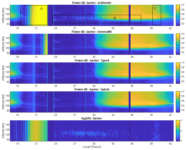
Figure 1 Range–time–intensity (RTI) plots of incoherent scatter total power returns on 11–12 September 2014. The first four panels, starting from the top, are the power return of the sample mean, the trimmed mean at the 95 % level, the trimmed mean based on the geometric deviation, and a hybrid method, respectively. The last panel is the normalized standard deviation.

Figure 1 shows the averaged power returns as a function of time and altitude using the sample, trimmed, T_GEO4, and hybrid means. Because the radar samples are in in-phase and quadrature pairs and larger N₁ contaminates more data samples, N₁ is chosen to be 2. The last panel shows the normalized standard deviation R(A_N) for the sample mean, whose expectation is 1 when there is no interference. For each data point, we first average 250 pulses using the method indicated in the title and then average four such groups arithmetically for a total of 1000 pulses. Using a smaller number of pulses makes the memory requirement less stringent and the trimmed mean more efficient. The ionosphere signal is largely characterized by smooth temporal and spatial variations during the daytime and by thin horizontal layers, known as sporadic E's, around 100 km at nighttime. The study of sporadic E layers and the associated dynamics have attracted much attention and are active areas of research (e.g., Mathews, 1998; Larsen et al., 2007; Wang et al., 2022; Kunduri et al., 2023). Two types of interference seen in Fig. 1 are represented in boxes A and B in the top panel. Box A is likely another radar operating at the same inter-pulse period (IPP) as that of the Arecibo ISR or is an internal system problem. Vertical lines in box B and other similar vertical lines that are confined to ∼90–120 km are meteoric echoes. The altitude extension of meteor echoes is because fast-moving meteor heads cannot be decoded by the matched filter. They do not extend beyond 120 km in altitude in our case because meteor echoes are detected below about 115 km (Zhou and Kelley, 1997). The normalized standard deviation R(A_N) is displayed in the bottom panel in Fig. 1.

The top panel in Fig. 1 shows the result of arithmetically averaging 1000 pulses (i.e., the sample mean). All types of interference show up prominently, as the method does not filter out any contamination. The trimmed mean (second panel) cleans up the first part of the heavy contamination in box A but is not effective against the second part, most likely because more than 5 % of the pulses were contaminated. T_GEO4 and the hybrid method largely filters out the contamination in box A and reveal the underlying sporadic layer despite the heavy contamination. Although T_GEO4 appears to handle all the contamination as well as the hybrid method does, it is slightly inferior to the latter in reducing statistical error, as seen in the later part of this section. The only residue contamination not filtered out is around 22:30 LT. None of the methods is effective in removing it completely, and all three robust estimators appear to perform the same. As the total power of the interference is relatively low, interference may permeate most of the pulses, making it very difficult to remove it from each pulse. For this type of interference, one way is to find the mean at non-ionosphere heights and subtract it from the entire profile. Noise samples are available at Arecibo. Background noise is not subtracted here to focus on the effect of robust estimators in this study. The trimmed mean, T_GEO4, and hybrid methods are all effective at removing meteor interference, which typically does not last more than 50 ms at Arecibo, i.e., 5 pulses (Zhou and Kelly, 1997).

Other than the most obvious interference highlighted in boxes A and B, no other contamination appears to be obvious. The R value in the region indicated by box C has elevated values, indicating likely contamination. Yet there appears to be little difference between the sample mean result in the top panel of Fig. 1 and the results from the robust estimators. One effect of the interference is that it increases the statistical error, which is more difficult to see from the RTI plot. To estimate the statistical error, we use the difference in the power minus the average power of the surrounding 15 points in height and 5 points in time as a proxy for the error. The square ratio of the sample mean error to the error in the hybrid method is displayed in Fig. 2a. The corresponding R(A_N) is displayed in Fig. 2b. Larger statistical error from the sample mean in the region indicated by box C in Fig. 1 is quite evident. Although R(A_N) is not linearly related to the error, elevated R(A_N) is a robust indicator of contamination. This is also evidenced from 01:00 to 03:00 LT in Fig. 2, where sporadic elevations of R(A_N) and statistical errors are seen to be correlated.

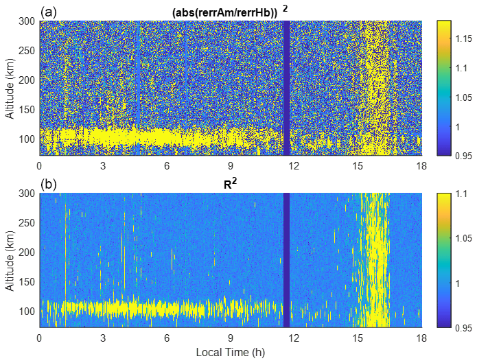
Figure 2 (a) The square of the relative error in the sample mean method normalized to that of the hybrid method. (b) The normalized variance. The yellow color in (a) indicates that the sample mean has a larger error than the hybrid method.

An estimator needs to be efficient when there is no interference. Figure 3 shows the ratio of the sample mean and T₉₅ errors to the hybrid error as well as the corresponding standard deviation R(A_N) averaged between 07:00 to 13:00 LT, during which period contamination is minimal above 120 km (as seen in Fig. 2). The error in the hybrid estimator is virtually the same as that in the arithmetic average. The error in the T₉₅ estimator is 1.036 times the error in the hybrid estimator, which is in good agreement with the simulated value of $\sqrt{\mathrm{1.09}/\mathrm{1.018}}=\mathrm{1.035}$. Similarly, the error in T_GEO4 is slightly smaller than that in T₉₅, which is also in good agreement with the simulation results shown in Table 1. The mean R(A_N) correlates with the elevated error in the region of 90–120 km. We also note that the mean R(A_N) above 120 km is 0.997, which is slightly below the expected value of 1. Although the deviation is small, it is statistically significant. This may be caused by the bias in the receiving channels or the finite dynamic range of the analog-to-digital converters.

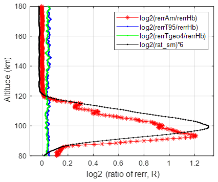
Figure 3 Mean relative errors (in base-2 logarithms) of the sample mean, trimmed mean, and T_GEO4 normalized to that of the hybrid method (red and blue lines, respectively). The black line is 6 times the logarithm (base 2) of the mean R. The time duration averaged for all the lines in the figure is from 07:00 to 13:00 LT on 12 September 2014.

3.2 Power spectrum processing and Doppler velocity comparisons

The power spectral density (PSD) of an ISR is obtained by transmitting a coded long pulse (CLP), 440 µ s in our case. The baud length is 2 µ s, making the bit number of the pulse 220. The inter-pulse period is 10 ms as in the Barker data. The bit sequence is random for each transmitted pulse. The PSD is obtained by the Fourier transform of the data multiplied by the complex conjugate of the code. The characteristics of the CLP are discussed by Sulzer (1986). The averaging of the PSD at each frequency component is identical to that of the total power in the above section, which can be viewed as the center frequency component.

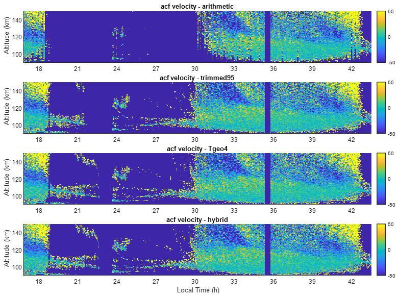
Figure 4 Vertical ion velocities obtained using the four estimators. The estimators, from top to bottom, are the sample mean, trimmed mean (at 95 %), T_GEO4, and hybrid mean, respectively.

Figure 4 shows the Doppler velocity derived from the four estimators using the phase of the auto-correlation function. The vertical ion drift in the altitude range of 90–150 km is typically less than 50 m s⁻¹ above Arecibo. Below 120 km, the plasma drift is the same as the neutral wind because of the complete coupling between ions and neutral molecules. During the daytime, there are sufficient signals above 95 km to obtain continuous spatial and temporal velocities. During the nighttime, it is only possible to obtain velocities within thin ionization layers. While ion velocity with fine height and time resolutions is of great geophysical interest (e.g., Zhou et al., 1997; Hysell et al., 2014), our focus here is to study the relative accuracy of the velocities obtained from different estimators.

Comparisons of the velocity results largely follow those of the total power. The sample mean fails in boxes A and B. Additionally, during the sunrise hours when the ionospheric signal is low and the meteoric interference is strong, the sample mean can only yield valid velocities occasionally while the robust estimators can obtain the velocities continuously in altitude and time. As in the total power estimation, the trimmed mean does not yield valid results in the second part of box A from 21:30 to 22:30 LT, while the hybrid and T_GEO4 methods appear not to be affected by the interference very much.

To compare the statistical fluctuations, we use the altitudinal difference in the velocity divided by the square root of 2 as a proxy for velocity error. Figure 5 shows the altitude variation in the velocity error during 08:00–10:00 LT as well as 14:30–16:30 LT on 12 September. All the robust estimators have essentially the same error at each altitude, while the sample mean has a much larger error around 100 km. The error in the sample mean converges to those of the robust estimators above 145 km. The diminishing error difference in the sample mean with increasing altitude is due to the long pulse length (440 µ s) used. A characteristic of the CLP pulse is that the interference at one altitude is uniformly spread across the entire bandwidth randomly at other altitudes. A meteor echo at 100 km increases the spectral power fluctuations with diminishing strength up to 166 km. Meteoric influx peaks at 06:00 LT and varies strongly with the local time. The daily variation in meteoric flux is quantitatively analyzed by Zhou et al. (1995) and Li and Zhou (2019). It can also be qualitatively seen in Fig. 2b. The larger error in the sample mean during 08:00–10:00 LT is a reflection of the strong meteoric flux. Although the afternoon period suffers from meteoric interference and radio contamination, as seen in Fig. 2, both of them are weak. Statistical averaging of 6000 pulses is able to even out the spectral power fluctuation to such a degree that all the estimators produce the same velocity. For spectral processing, the most important factor is the total amount of noise power, while the percentage of pulses contaminated is often more important in total power processing.

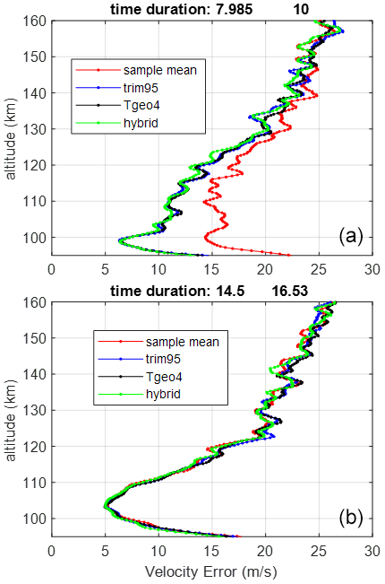
Figure 5 Doppler velocity errors for the sample mean, trimmed mean, T_GEO4, and hybrid method on 12 September 2014 for 08:00–10:00 LT (a) and 14:30–16:30 LT (b).

Overall, we see that the T_GEO4 and hybrid estimators accurately and consistently improve velocity and total power measurements over the sample mean, which are important for studying the E-region dynamics and composition. The availability of nighttime velocities will help reduce the large error in the measurement of atmospheric tides in the E region (Zhou et al., 1997; Gong et al., 2013). Accurate measurement of the power spectrum and total power will facilitate all E-region studies, especially those concerning the climatology and dynamics of sporadic E and intermediate layers (Zhou et al., 2005; Hysell et al., 2009; Raizada et al., 2018; Gong et al., 2021). Of particular importance are the vertical wind and ion composition of the E region, which have not been studied much due to a lack of quality data.

4 Summary and conclusion

We have discussed several robust estimators to compute the variance of a normally distributed random variable, X, to deal with interference. This variance is the same as the mean of the power variable, X². The effectiveness of an estimator is described by the normalized standard deviation, R. We derive the theoretical R values for the median, geometric mean, and trimmed mean of gamma distributions, which result from averaging the power random variables. We discuss and compare another four estimators through simulations for various interference scenarios. Robust estimators found in the literature are typically rank-based (e.g., the median, trimmed mean, and median absolute deviation). We have used the geometric mean and geometric deviation as two basic parameters in assessing the likelihood of a data point being contaminated. The methods based on the geometric mean have two advantages over the rank-based ones: they are less susceptible to the large uncertainties in the tail part of the distributions and they are computationally more efficient. For the interference model used, the T_GEO4 estimator, which is based on the geometric mean, is particularly effective as a stand-alone estimator when there is no initial average. Another effective estimator based on the geometric mean is the weighted mean. The R value of the sample mean can be used to assess whether the process conforms to the expected distribution. This knowledge allows us to combine the sample mean with other robust estimators to mitigate contamination and achieve statistical accuracy.

We apply three robust estimators to incoherent scatter power and velocity processing, along with the traditional sample mean estimator. We show that the performance of estimators with real data agrees well with simulations. In the total power processing, the trimmed mean performs mostly well except when the contamination is very heavy. The T_GEO4 estimator performs almost as well as the hybrid method in mitigating interference. The hybrid method performs the best at mitigating interference as well as at reducing statistical errors. For Doppler velocity processing, the same conclusion can be drawn in cases of frequent interference. When the interference is weak, all the robust estimators appear to perform well. For the Arecibo ISR data, the sample mean has larger statistical errors even for data that may not appear to contain obvious interference. This highlights the need for robust estimation to process or reprocess decades of E-region data taken at Arecibo. The hybrid estimator is most advantageous under all circumstances. This conclusion is likely applicable to other incoherent scatter radars as well. While the interference characteristics differ at each radar site, the study provides a foundation to optimize robust estimation, which is an essential step in many data processing applications.