the Creative Commons Attribution 4.0 License.
the Creative Commons Attribution 4.0 License.
 | 17 Jul 2024
Using metal oxide gas sensors to estimate the emission rates and locations of methane leaks in an industrial site: assessment with controlled methane releases
Rodrigo Rivera-Martinez
Pramod Kumar
Olivier Laurent
Gregoire Broquet
Christopher Caldow
Ford Cropley
Diego Santaren
Adil Shah
Cécile Mallet
Michel Ramonet
Leonard Rivier
Catherine Juery
Olivier Duclaux
Caroline Bouchet
Elisa Allegrini
Hervé Utard
Philippe Ciais
Fugitive methane (CH4) emissions occur in the whole chain of oil and gas production, including from extraction, transportation, storage, and distribution. Such emissions are usually detected and quantified by conducting surveys as close as possible to the source location. However, these surveys are labour-intensive, are costly, and fail to not provide continuous emissions monitoring. The deployment of permanent sensor networks in the vicinity of industrial CH4 emitting facilities would overcome the limitations of surveys by providing accurate emission estimates, thanks to continuous sampling of emission plumes. Yet high-precision instruments are too costly to deploy in such networks. Low-cost sensors using a metal oxide semiconductor (MOS) are presented as a cheap alternative for such deployments due to their compact dimensions and to their sensitivity to CH4. In this study, we demonstrate the ability of two types of MOS sensors (TGS 2611-C00 and TGS 2611-E00) manufactured by Figaro® to reconstruct a CH4 signal, as measured by a high-precision reference gas analyser, during a 7 d controlled release campaign conducted by TotalEnergies® in autumn 2019 near Pau, France. We propose a baseline voltage correction linked to atmospheric CH4 background variations per instrument based on an iterative comparison of neighbouring observations, i.e. data points. Two CH4 mole fraction reconstruction models were compared: multilayer perceptron (MLP) and second-degree polynomial. Emission estimates were then computed using an inversion approach based on the adjoint of a Gaussian dispersion model. Despite obtaining emission estimates comparable with those obtained using high-precision instruments (average emission rate error of 25 % and average location error of 9.5 m), the application of these emission estimates is limited to adequate environmental conditions. Emission estimates are also influenced by model errors in the inversion process.
- Article
(15409 KB) - Full-text XML
- BibTeX
- EndNote


A recent study suggests that in the decade 2008–2017, methane (CH4) emissions from the production, transportation, storage, and distribution of fossil fuels (e.g. coal, oil, and natural gas) accounted for 35 % of global anthropogenic CH4 emissions (Saunois et al., 2020). These emissions are typically quantified through emission inventories. Emissions estimates reported by inventories rely on information from activity data (i.e. human activities contributing to emissions like fuel consumption) and emission factors (i.e coefficients that relate the activity data to emission rates). Although generalised emission factors can be used to develop emission inventories, emission factors can vary between different sites depending on site-specific technologies and operating modes, which makes the upscaling of fugitive CH4 emissions highly uncertain (Alvarez et al., 2018). For instance, estimated emissions from the oil and gas supply chain in the US in 2015 constrained from ground-based and aircraft measurements were found to be 60 % higher than the Environmental Protection Agency (EPA) inventory (Alvarez et al., 2018). More generally, the characterisation of CH4 emissions from complex processes based on generalised emission factors can be underestimated when best practices are not followed by operators (Riddick et al., 2020).
Atmospheric measurements are increasingly used to detect and quantify CH4 leaks from industrial facilities. These methods primarily involve measuring methane mole fraction downwind of the facility. Measurements are often interpreted with local-scale dispersion models using atmospheric inversion methods to infer the CH4 source location and emission rate; see e.g. Kumar et al. (2022). Current approaches generally consist of conducting atmospheric surveys of the enriched mole fraction plume created by the emitting source. There are several challenges with this approach: accessibility to sample downwind emission plumes, labour requirements, and instrument costs, given that surveys may employ expensive high-precision research-level CH4 instruments using techniques such as cavity ring-down spectrometry (CRDS). Further, downwind surveys do not provide continuous source monitoring (Travis et al., 2020). The deployment of networks of continuous monitoring CH4 sensors around emission sources is an alternative to surveys, but the costs of each instrument remain a limitation. Advances in the development of low-cost sensors facilitates the deployment of dense sensor networks to increase site coverage (Kumar et al., 2015; Mead et al., 2013). The use over long periods of time of dense networks of sensors deployed permanently increases the ability to identify the structures of the observed plumes, to improve the atmospheric transport modelling parameterisation for the simulation of these plumes, and thus to improve the accuracy of the quantification of the leaks based on this modelling.
In recent years, growing interest in low-cost and low-power sensors for use in relatively dense networks has led to the study of different kinds of sensors to measure pollutants and trace gases like carbon dioxide (CO2) or CH4. One of the most common low-cost-sensor technologies for the detection and quantification of CH4 emissions is metal oxide semiconductors (MOSs). MOS sensors are composed of a metal oxide sensing material, incorporating an integrated heater. A chemical reaction affects the electrical conductivity of the sensing material in the presence of an electron donor gas such as CH4 (Örnek and Karlik, 2012). However, MOS sensor sensitivity is also affected by other environmental parameters such as temperature and relative humidity (Popoola et al., 2018); they also present low accuracy and may drift with time (in the form of a decrease in the conductivity of the sensing material), requiring periodic re-calibrations (Riddick et al., 2020; Shah et al., 2023, 2024) and the need for a constant power supply due to the heater material (Shah et al., 2023).
The Taguchi gas sensor (TGS) is a commercially available range of MOS sensors manufactured by Figaro®, which have been widely tested in different environments (including under controlled conditions and during field deployment) due to the CH4 sensitivity of certain TGS models (Eugster et al., 2020; Eugster and Kling, 2012; Riddick et al., 2020; Collier-Oxandale et al., 2018; Bastviken et al., 2020; van den Bossche et al., 2017; Shah et al., 2023, 2024). A standard technique for calibrating these sensors has involved collocating them with a high-precision instrument used as a reference, and then applying empirical equations or data-driven approaches to derive CH4 mole fraction (Eugster et al., 2020; Eugster and Kling, 2012; Casey et al., 2019; Bastviken et al., 2020; Collier-Oxandale et al., 2019, 2018). In a previous work (Rivera Martinez et al., 2021) we studied the possibility of using artificial neural networks (ANNs) to reconstruct variations in CH4 mole fractions in room air under controlled conditions from three types of Figaro sensors (TGS 2600, TGS 2611-C00, and TGS 2611-E00). A following study (Rivera Martinez et al., 2023a) analysed the potential to reconstruct CH4 spikes generated on top of ambient air observations, which corresponded to typical signals from leaks at industrial sites, employing two types of Figaro sensors (TGS 2611-C00 and TGS 2611-E00). That study made a comprehensive comparison of the performance of five models for the reconstruction of CH4 mole fraction.
The next logical step is to test the performance of the same sensors to reconstruct CH4 mole fraction from real leaks and to use reconstructed mole fractions to quantify and localise emission rates. Riddick et al. (2020) quantified CH4 emissions from a gas terminal using a Figaro TGS 2600, deployed 1.5 km from the emission source. To reconstruct CH4 mole fractions from voltage observations, the authors developed an empirical equation considering the measured voltage, temperature, and relative humidity from a nearby meteorological station and then applied a Gaussian plume model to quantify the emission rate using reconstructed CH4 mole fractions and local wind information. Their estimated average emissions were 9.6 g CH4 s−1, with a maximum emission rate of 238 g CH4 s−1, given corresponding CH4 mole fraction enhancements of between 2 and 5.4 ppm within the plume. Their Figaro-based emission estimates were not confronted with corresponding emission estimates derived using a high-precision gas analyser or with independent knowledge of the emission rate. Elsewhere, Riddick et al. (2022) studied the capabilities to detect and estimate CH4 emissions of four Figaro TGS 2611-E00 sensors in a fence-line monitoring setup. Sensors were deployed closer to the emission source (30 m) and tested over a 48 h period. Reported results showed detection consistency for emissions above 167 g CH4 h−1 with an enhancement threshold of 2 ppm. However, the number of sensors used to compute the emission estimates was not specified, particularly given the spatial distribution of the sensors and varying wind speed.
In this study, we test the ability of a network of several Figaro sensors to reconstruct atmospheric CH4 mole fraction enhancements from a series of controlled releases of known magnitude and duration to the open atmosphere at a facility called TADI (see Methods) and to infer the emission rate of each release by an inverse modelling approach. The accuracy of CH4 mole fraction reconstruction is evaluated against collocated accurate CH4 measurements from high-precision CRDS instruments. The accuracy of the inverted emission locations and rates is evaluated against the known (controlled) location and magnitude using the inversion model of Kumar et al. (2022).
This study builds upon the research conducted by Rivera Martinez et al. (2023a) and Kumar et al. (2022), demonstrating the potential for continuous monitoring of CH4 emissions using cost-effective in situ sensors. Drawing from the insights derived from these two studies, this study seeks to address the new challenges associated with the combination of both types of analysis, i.e reconstruction of CH4 mole fractions from measured voltage variations and estimation of emission rates and location from CH4 mole fractions. Firstly, the challenge arises in the deployment and management of onsite Figaro sensors, an issue not present in Rivera Martinez et al. (2023a), as well as extracting CH4 mole fractions from measurements that are impacted by more complex perturbations. For instance, the background air in Rivera Martinez et al. (2021, 2023a) was less polluted than air from an industrial site such as TADI. Moreover, the environmental conditions, especially in terms of temperature and water mole fraction, in these previous studies were smooth and not representative of field conditions as encountered in this new study. Secondly, the prescriptive precision and accuracy targets for CH4 reconstructions outlined in Rivera Martinez et al. (2023a) were established as generic targets, fitting for a variety of data processing strategies intended to quantify emissions from industrial sites. The specific observation and modelling strategy implemented in Kumar et al. (2022) to localise and quantify point source emissions carries its own set of precision/accuracy requirements. In particular, this strategy strongly relies on the characterisation of gradients across measurement stations of mole fraction averages over time or wind sectors, which makes the derivation of nominal requirements on the reconstruction of CH4 spikes or the CH4 time series quite complex. Furthermore, such requirements should be weighed against the modelling uncertainties associated with the corresponding Gaussian plume model inversions. Ideally, the uncertainties related with CH4 mole fraction data would not significantly contribute towards the total uncertainty when combined with uncertainties from the modelling framework. This, however, does not necessarily mean that they should be much smaller than the latter. The direct comparison of the results obtained in this study with CH4 mole fraction data derived from Figaro sensors and those from Kumar et al. (2022) provides insights into whether this objective is achieved.
Therefore, for 33 controlled releases at the TADI facility, we employed fixed-point measurements from both high-precision CRDS instruments and low-cost TGSs. A considerable fraction of the TGS measurements were used for training models to reconstruct CH4 mole fractions from measured TGS resistance and other variables. When reconstructing CH4 mole fractions, we proposed a minimum accuracy target of 15 % of the amplitude of the largest observed mole fraction enhancement within a release. This corresponds to accuracies from 0.3 ppm for a release causing a maximum enhancement of 2.4 ppm up to 18 ppm for a maximum enhancement of 120 ppm. This accuracy is consistent with the accuracy requirement imposed in our previous study where we used TGS sensors to reconstruct CH4 spikes created in a laboratory experiment (Rivera Martinez et al., 2023a). However, the relevance of this target is implicitly re-assessed through the use of the reconstructed time series in the inversion scheme from Kumar et al. (2022).
The plan of the study is as follows. Section 2 presents the TADI 2019 controlled releases campaign, the logger systems, the data treatment, the models employed to reconstruct CH4 concentration from TGS data, and the atmospheric inversion approach. The comparison of the models for the reconstruction of CH4 and the inversion results for rates and locations of different releases are analysed in Sect. 3. Results are discussed in Sect. 4, and conclusions are given in Sect. 5.
2.1 TADI-2019 campaign
In October 2019, TotalEnergies® performed multiple controlled releases at the TotalEnergies Anomaly Detection Initiative (TADI) facility to investigate the capability of different detection and quantification techniques of CH4 emissions from industrial facilities. The TADI test site is located northwest of Pau, France, with an approximate area of 200 m2. It is equipped with infrastructure typical of oil and gas facilities (pipes, valves, tanks, etc.) to simulate realistic leaks. The terrain is flat but includes different obstacles that can affect the dispersion of the gases released to the atmosphere. Our experiment consisted of 41 controlled releases of CH4 and CO2, covering a wide range of emission rates of between 0.15 and 150 g CH4 s−1, with durations ranging between 25 and 75 min. We participated in this experiment to develop and test inverse modelling frameworks within the TRAcking Carbon Emissions (TRACE, https://web.archive.org/web/20230824195644/https://trace.lsce.ipsl.fr/, last access: 11 March 2023) programme for the estimation of emission location and rates based on CH4 mole fractions from high-precision instruments (Kumar et al., 2022). We presented the inversion results for 26 releases from single point sources based on two inversion approaches, one relying on fixed-point measurements and the other one on mobile near-surface measurements (the latter had already been documented in Kumar et al., 2021). In both cases, the emission estimates relied on CH4 mole fractions from high-precision instruments and on a Gaussian plume model to simulate the local atmospheric dispersion of CH4. The results from Kumar et al. (2022) for point source emissions yielded an emission rate error of between 23 % and 30 % and a localisation error (within a 40 m × 50 m area) of between 8 and 10 m. The controlled releases were emitted from heights of between 0.1 and 6 m above ground level and inside the 40 m × 50 m ATEX (ATmospheres EXplosibles) zone of the TADI facility (see Fig. 1).
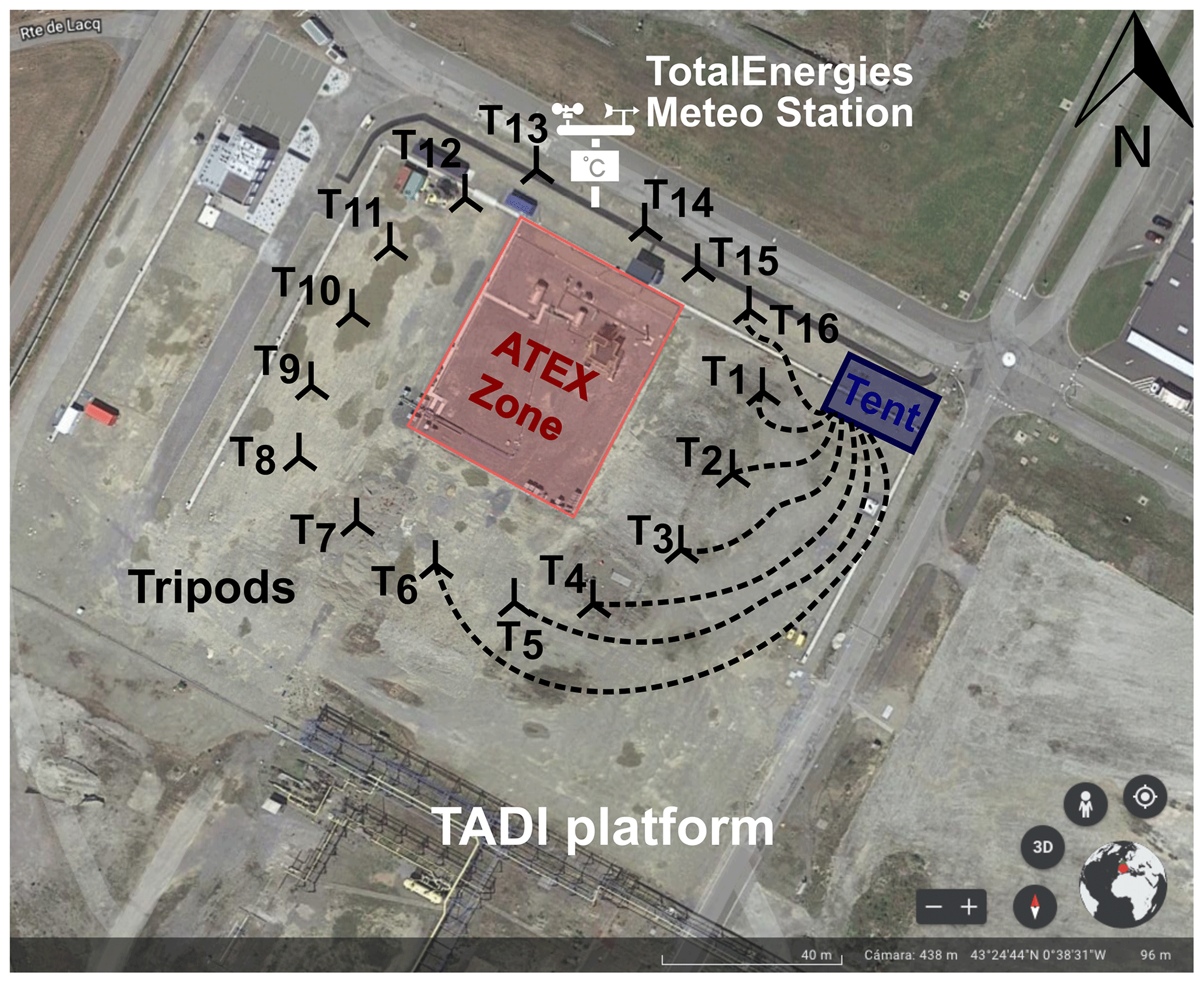
Figure 1Diagram of the experimental setup on top of a satellite image of the TADI platform (source: © Google Earth). The locations of the releases are inside the red rectangle (ATEX zone). The locations of the 16 tripods are presented as black symbols and denoted with Tx, where x is the index of the tripod from 1 to 16. The blue rectangle indicates the tent location. Examples of the sampling lines connecting the tripods to the tent are shown as dashed lines, only showing 7 of 16 in total. The white symbol shows the location of the Meteorological station installed by TotalEnergies®.
2.2 Controlled releases and sampling configuration
A total of 41 controlled releases were conducted over a 7 d period, between 2 and 10 October 2019. Six releases corresponding to low wind speeds (< 0.6 m s−1) were not used for the inversion as in Kumar et al. (2022), since measurements made in low winds are not suitable for atmospheric inverse modelling. They could, however, be used in the training of CH4 mole fraction reconstruction models. The two largest releases produced high CH4 mole fraction plumes that affected the amplitude measured by the TGS sensors, such that it was not possible to distinguish large CH4 spikes from medium and small spikes from voltage drop measurements (see Fig. A3), and, hence, they were also removed. Therefore, our study is focused on 33 from the initial 41 controlled releases conducted during the campaign. Table A1 details the releases that were measured by each chamber. The protocol followed in the selection of releases used for the training and testing of reconstruction models is explained in Sect. 2.6.
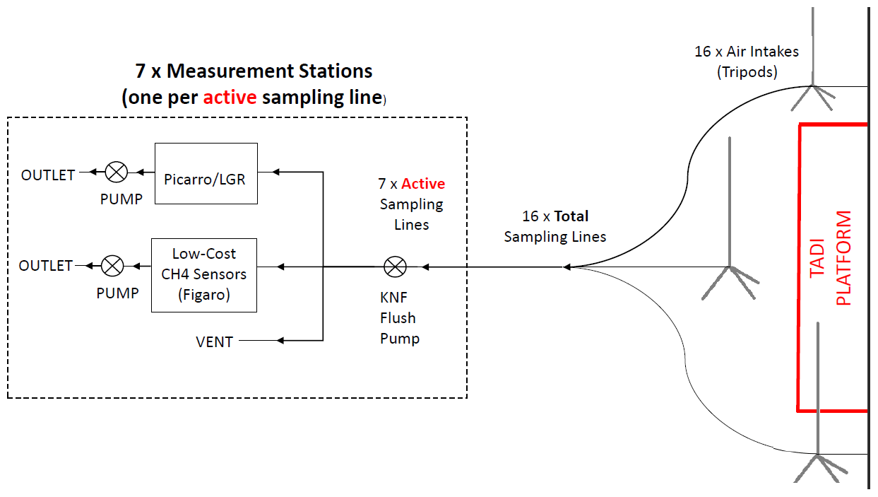
Our atmospheric sampling configuration for measuring CH4 is shown in Fig. 2. It consisted of placing 16 sampling lines (of 6.35 diameter) on the ground, with one end of each line attached to tripods of between 2.75 and 3.50 m high around the ATEX zone, serving as air inlets, and the other end of each line connected to a pump flushing at 6 L min−1 (KNF N811 with PTFE diaphragm). The lengths of the sampling lines varied from 10 to 100 m, connecting each air inlet to the CH4 sensors inside a tent. The pump was connected upstream of the high-precision instruments (Picarro CRDS or LGR), a chamber containing a series of TGS CH4 sensors, and other environmental sensors measuring relative humidity, pressure, and temperature. To maintain the inline pressure at atmospheric pressure, a vent was also connected to each sampling line (Fig. 2). Table A5 summarises the species measured and the identifiers of the reference high-precision instruments. All reference instruments measured H2O to provide dry gas mole fractions. The analysers' sampling frequency ranges between 0.3 and 1 Hz. In a previous study by Yver-Kwok et al. (2015), it was proven that these CRDS gas analysers ensure high-precision measurements and a low drift over time, of less than 1 ppb per month, although the data sheet specifies a drift of 3 ppb per month (Picarro Inc., Santa Clara, CA, USA).
On average six sampling lines were active for each release, with each active line being connected to a high-precision instrument and a TGS chamber. The lines were activated depending on wind direction. The strategy behind the distribution of the tripods around the emitting area and for the inversion was to continuously acquire several measurement points within the plume generated by each release, in addition to one or a few measurement points outside the plume (to characterise the background mole fraction level upon which plumes enhancements can be assessed) for each release, regardless of the wind conditions (Kumar et al., 2022).
2.3 Low-cost CH4 sensor logger system and meteorological data
Seven chambers containing TGS sensors were used. Table A6 shows the TGS and environmental sensors in each chamber, as well as the type of chamber. Each chamber contained at least three TGS units with voltage measurements sensitive to CH4 and two other sensors measuring relative humidity/temperature and pressure/temperature. All sensors were inserted inside an acrylic/glass or steel/glass chamber with volumes of 100 and 120 mL, respectively. The logger system design was previously documented on Rivera Martinez et al. (2021, 2023a). The measurement sensitivity of the TGS signal was determined by a load resistor connected in series with the sensor (Figaro®, 2013, 2005); the load resistance was either 5 kΩ or 50 kΩ (see Table A6). An AB Electronics PiPlus ADC board mounted on a Raspberry Pi 3B+ recorded the voltage drop across the load resistor, providing observations every 2 s. These voltage data are used for the characterisation and reconstruction of the CH4 signal. Consistency was observed between the two TGS 2611-E00 sensors installed in chamber E, and only one sensor of this type is used in this study.
Measurements of environmental parameters from all chambers other than chamber E had data gaps or recorded poor data for extended periods, including during releases, and were therefore not used. This study focuses on reconstructing CH4 using data from TGS 2611-C00 and TGS 2611-E00 from chambers A, C, D, E, F, and H. TGS 2600 data were discarded since this sensor did not respond to most of the CH4 peaks during the releases (see Fig. A1).
Table 1Summary of the information for the controlled releases with single CH4 point sources during the TADI 2019 campaign. Rows in bold font highlight releases with low-wind-speed conditions.
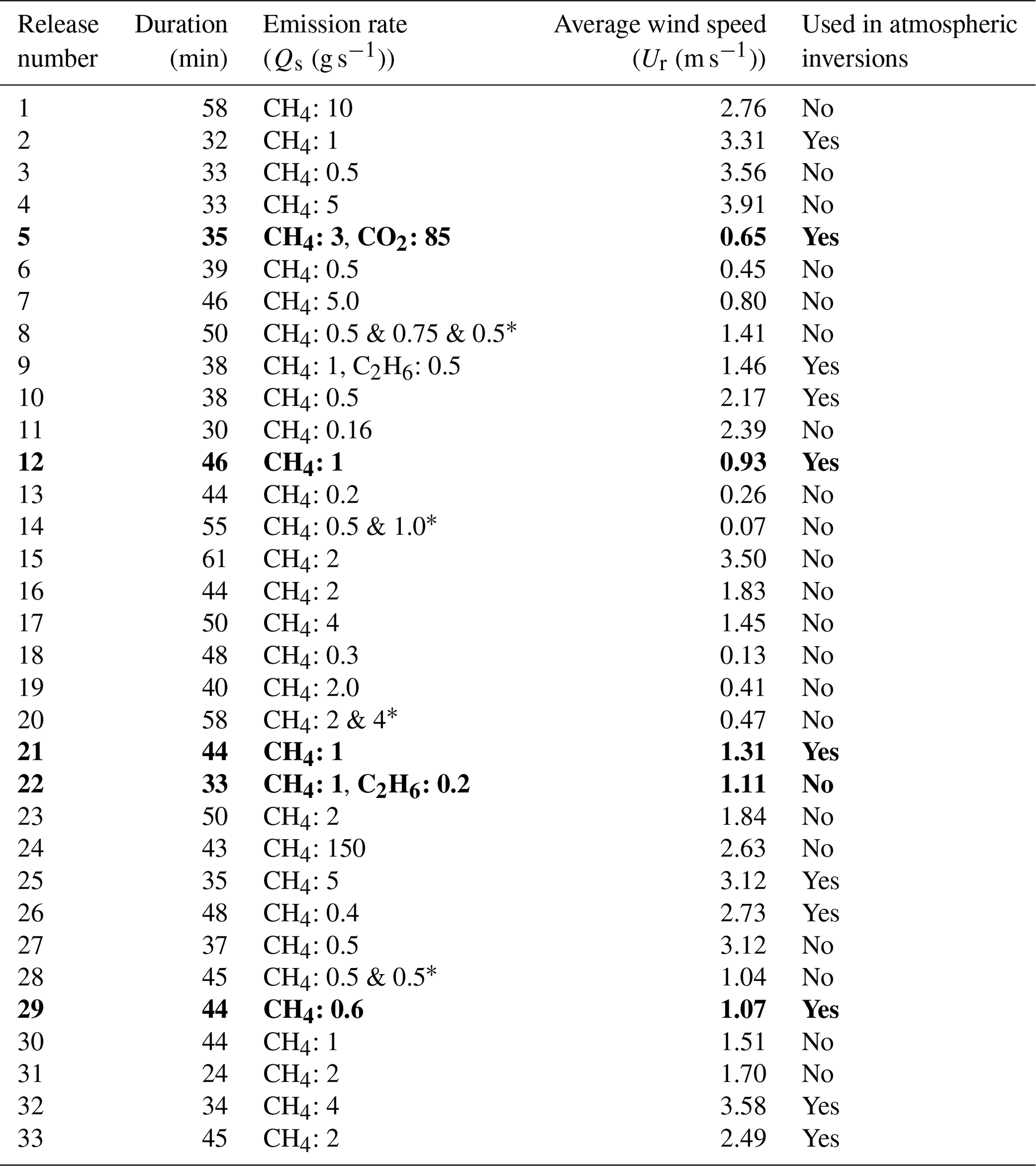
∗ Multiple source releases.
A meteorological station was installed on the TADI platform by TotalEnergies®, with a 3D sonic anemometer at 5 m above ground level (see Fig. 1), providing 1 min averages of wind speed (Ur) and wind direction (θ), and of the standard deviation of wind speed on the three axes (σu, σv, and σw). The data of turbulence and meteorological conditions are used in the dispersion model. Table 1 gathers general information for each of the 33 controlled releases during which we have valid TGS measurements: the duration of the release, the controlled release rate, the average wind speed over the duration of the release, and their inclusion status for inverse modelling.
2.4 Pre-processing of data from the TGS sensors
As well as resampling original observations with a 2 s time step to a longer 5 s time step, we also corrected the time offset due to air travelling from the air intakes to the instruments and the time delay from synchronisation between high-precision gas analysers and TGS chambers (between 2 and 3 min). We removed invalid TGS chamber data due to logging system faults. Finally, a baseline voltage correction was applied to the data from each sensor considering the entire campaign. Figure 3 illustrates the impact of the baseline correction, showing an improved agreement between corrected TGS voltage drop measurements for chamber A (for example) after the pre-processing steps and corresponding measurements from the reference gas analyser for one release.
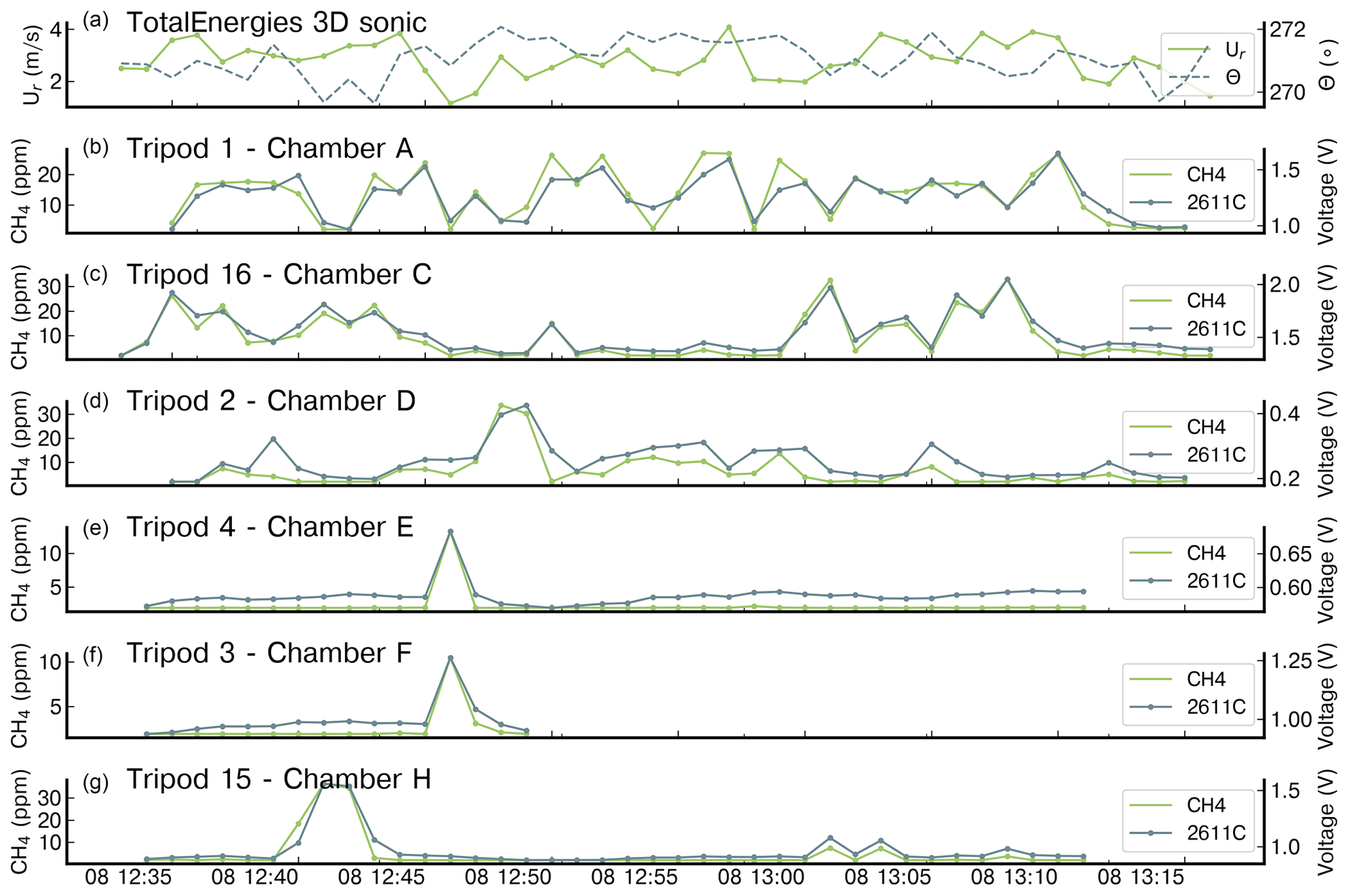
Figure 3An example of 1 min averaged CH4 mole fraction (ppm) and voltage drop (V) measurements, respectively, obtained from six high-precision instruments and one type of TGS sensor (TGS 2611-C00) for release 25 (Qs = 5 g s−1). CH4 measurements from the high-precision instruments are denoted as “CH4”, and the voltage measurements from TGS sensor are denoted as “2611C”. The top panel shows the 1 min averaged wind speed (Ur) and wind direction (θ) measured by the 3D sonic anemometer.
2.5 Reconstruction of spikes in CH4 mole fractions caused by the releases
The TGS chambers captured different segments of the plume with variations at high frequencies due to the distribution of the tripods with regard to the variable wind direction and due to atmospheric turbulence. The typical signal measured by the chambers shows a series of voltage enhancements, ranging between ∼ 1 and ∼ 15 min, corresponding to the plume lying over a slowly varying background signal associated with remote emissions. The targeted signal is that of the difference between the spikes and the background CH4 mole fraction level (Kumar et al., 2022). As an example, Fig. 3 shows 1 min averages of CH4 mole fractions measured by the reference instruments and the voltage from the TGS 2611-C00 at six tripods during release no. 25 (Qs = 5 g s−1), showing consistency between measurements from the reference instrument and corresponding voltage drop measurements from the TGS chambers. Chambers A, C, and D were in the trajectory of the plume or very close to it, measuring peaks of up to ∼ 30 ppm. Chambers E and F only captured a single peak of ∼ 10 ppm, and chamber H captured one large peak of ∼ 30 ppm. The mean wind speed during this release was 3.12 m s−1, with small wind direction variations of between 270 and 272°.
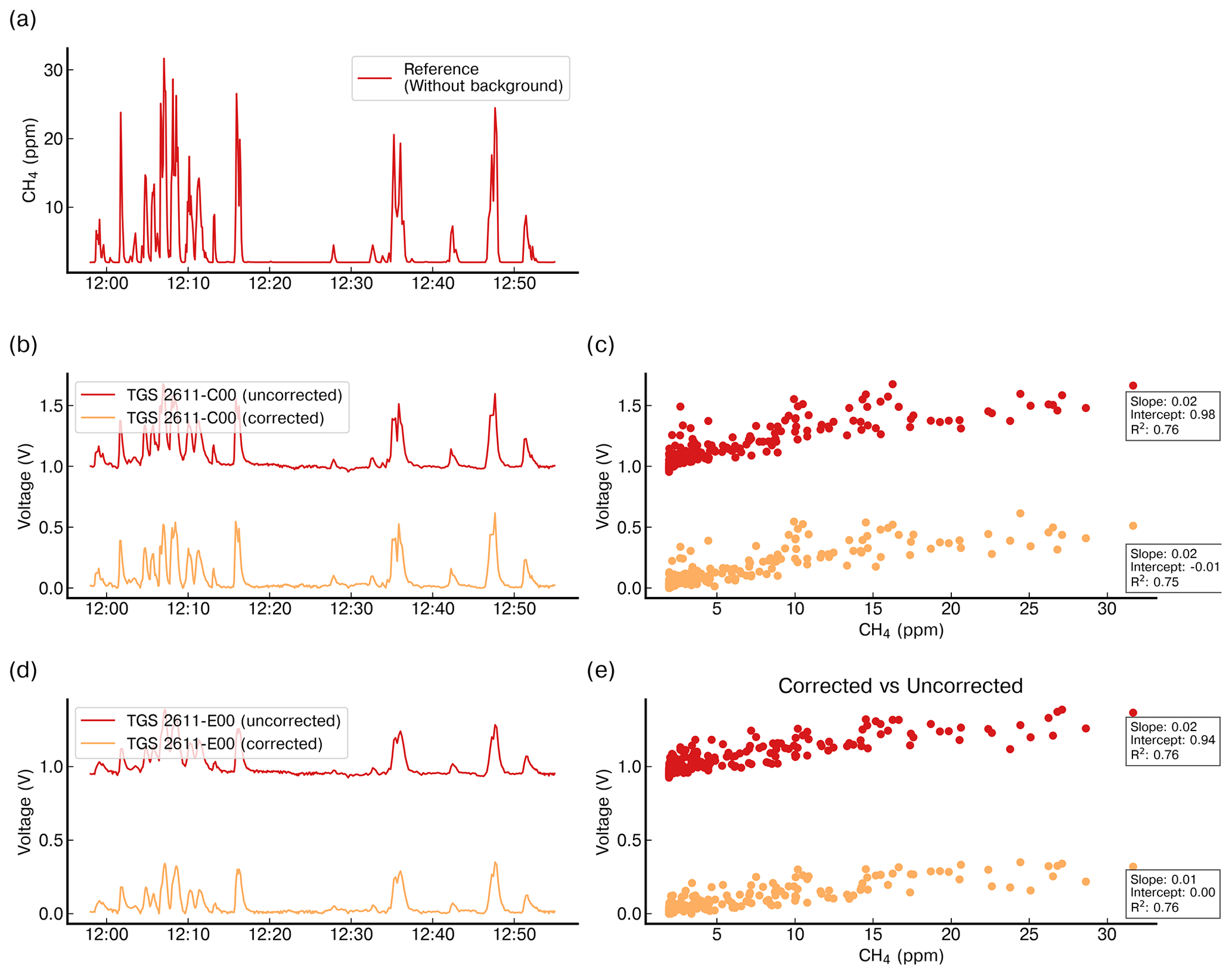
Figure 4Comparison of the voltage signal for one release (no. 8) from chamber A before (uncorrected) and after (corrected) the baseline correction on (b) TGS 2611-C00 and (d) TGS 2611-E00, on which the correction of the offset preserving the amplitude enhancements linked to CH4 variations is appreciated. Scatter plot of the corrected (orange) and uncorrected (red) signal vs. the reference CH4 observations for (c) TGS 2611-C00 and (e) TGS 2611-E00. (a) Reference CH4 mole fractions, also corrected using the spike correction algorithm.
TGS sensors are known to be sensitive to variations in humidity (H2O mole fraction) and temperature (T), affecting mainly the reconstruction of CH4 baseline (i.e. when sampling background air without CH4 enhancements) and thus the characterisation of peaks above this baseline (Rivera Martinez et al., 2021, 2023a). Two approaches can be used to correct for the effect of variable H2O mole fraction and T on the TGS voltage baseline signal and separate the voltage spikes from the baseline data in the time series. The first method consists of using H2O mole fraction (retrieved from relative humidity, pressure, and temperature) and T to correct the TGS voltage baseline signals. The second method involves the detection of voltage peaks associated with CH4 spikes and deriving a baseline with a linear interpolation on non-peak voltages. Due to logging issues in some chambers, we did not have complete relative humidity, pressure, and T data, which impeded us in defining a correction model. Therefore, in this study we employed the second approach. Figure 4 shows a comparison of the baseline correction for one release on voltage measurements of the TGS 2611-C00 and TGS 2611-E00 sensors. A comparison of both methods is shown in Fig. A2, justifying our choice.
To reconstruct CH4 mole fraction from TGS voltage measurements, we calibrated empirical models that derive relationships between TGS voltage and other input variables, compared to CH4 mole fraction measurements made by the high-precision gas analysers. The models are first calibrated (trained) and then evaluated (tested) using two independent subsets of data. To prevent a difference in the range of magnitudes from conditioning the determination of model parameters, the input variables are standardised, we applied a robust transformation consisting in removing the median and dividing input observations by their 1–99th quantile range. We selected the two reconstruction models that gave the best performance in our previous study (Rivera Martinez et al., 2023a), namely a polynomial regression and a multilayer perceptron (MLP) model. A description of the models and hyperparameter values (i.e. tunable parameters that influence the learning process of the model but not inferred from the data) are presented in SM. Three configurations of input variables were tested: (i) only with the TGS 2611-C00, (ii) only with the TGS 2611-E00, and (iii) with both TGS sensors sampling simultaneously. The results are shown in Sect. 3.1. To assess the performance of the reconstruction models to provide dry CH4 mole fraction enhancements (above the background) from voltage drop measurements corresponding to the TGS sensors, we used a normalised root mean square error (NRMSE) per release, weighted by the inverse of the maximum peak present in the release, defined as follows:
where yi are the CH4 mole fraction measurements provided by the high-precision instrument, are the reconstructed CH4 mole fractions, n is the number of observations present in each release, and hmax is the amplitude of the maximum mole fraction peak enhancement present in the release after removing the background. This normalisation allows us to compare performance across the different releases.
As mentioned, the target signal in this study is CH4 enhancements above the atmospheric background. We obtain this signal by subtracting the raw voltage signal during the release from an inferred baseline voltage computed using the peak detection algorithm and a linear interpolation.
We establish that an acceptable notional target error for reconstruction models should be below 15 % of the maximum spike amplitude during the release period, which translates to a NRMSE ≤ 0.15.
2.6 Selection of the training and test subsets for the reconstruction of CH4 mole fractions as input of the atmospheric inversion of emissions
Defining an appropriate training data set is important to allow reconstruction models to derive sufficient information to generalise (i.e. to extend its performance to data not present in the training set) and to obtain good mole fraction reconstruction performance in the testing data set. In addition, the testing data set should be chosen to allow for the evaluation of model performance under a wide variety of conditions. Regarding inverse modelling, in order to provide a meaningful assessment of the estimation of emission rates and locations, inversion should be conducted using reconstructed CH4 mole fractions from outside the training data set to avoid introducing bias in the evaluations of errors. Furthermore, depending on the magnitude of emission release rates, atmospheric turbulence, and locations/distances of the downwind active tripods from the emission sources, each of the six chambers could not be used to detect CH4 mole fractions during each release; therefore, a separate training and test set needs to be defined for each chamber.
Table 2Summary of the releases included in the training data set and testing data set of the CH4 reconstruction models. The mole fractions modelled for the test set are also used as input of the inversion model to infer the CH4 emission rate and their location.
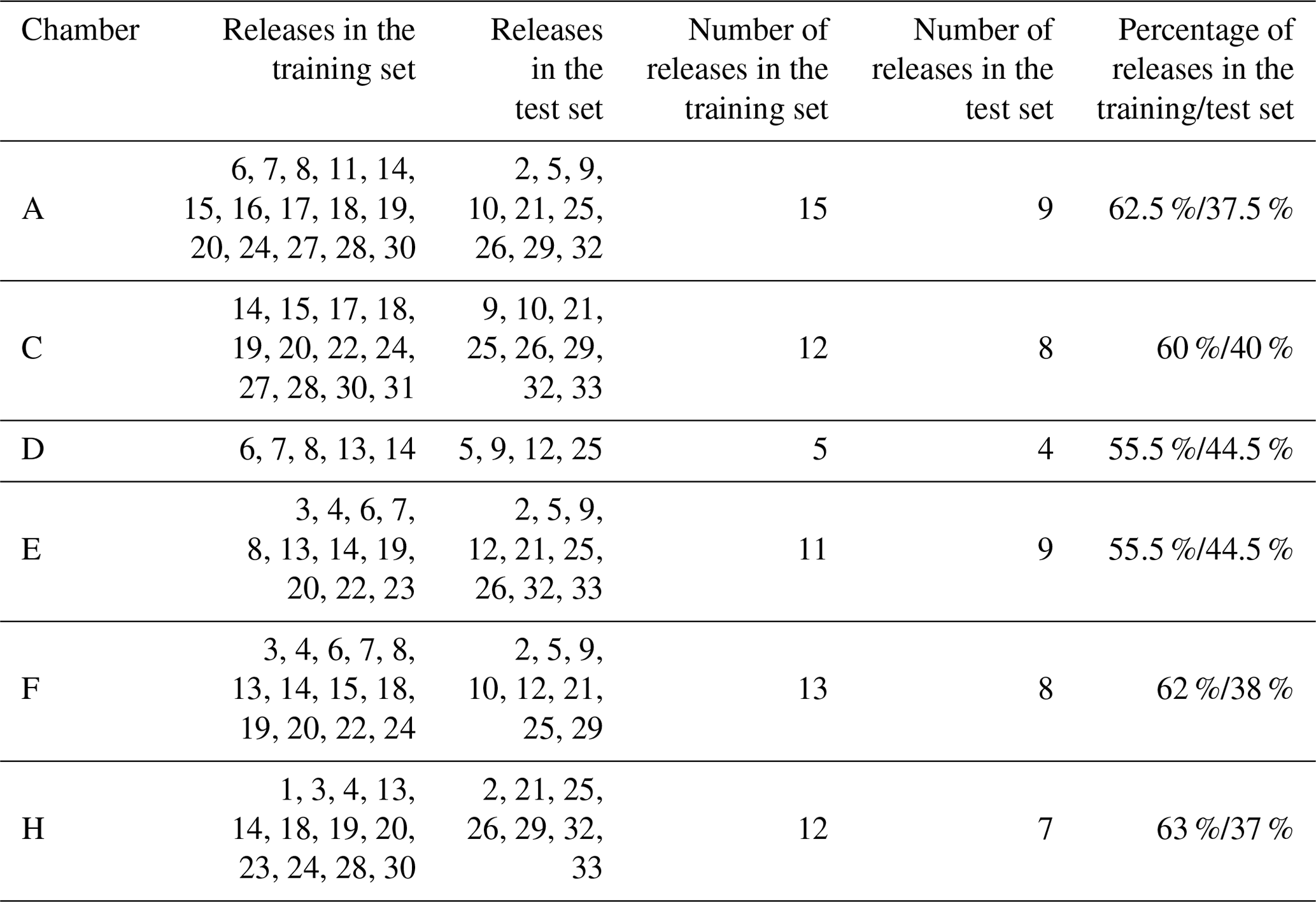
These previous considerations constrain the selection of the training and testing data sets from each chamber. The testing data set of the releases for use in inversions was defined based on two criteria: (1) releases which yield reconstructed CH4 mole fractions from at least three chambers simultaneously and (2) releases corresponding to the more favourable wind speed conditions (Ur ≥ 1.4 m s−1) for inversions. We determined seven releases that meet these considerations (no. 2, 9, 10, 25, 26, 32, and 33). Because this testing data set was of insufficient size for all of the chambers, we decided to increase it by using data from four more releases with low-wind-speed conditions (0.65 ≤ Ur ≤ 1.31) (no. 5, 12, 21, and 29). This selection led to a testing data set of 40 % of the releases. All remaining data were used as a training data set. The reconstruction models were trained and tested only once per chamber, following the distribution of the releases from Table 2.
2.7 Atmospheric inversion of the release locations and emission rates
Derivation of release locations and emission rates relies on an atmospheric inversion framework developed and tested by Kumar et al. (2022), which is based on measurements from high-precision instruments. The details of the approach and implementation for this atmospheric inversion framework are given in this publication, and they are just briefly summarised here. This framework processes averages of the time series of the observed CH4 mole fraction enhancements above the background from the different stations: from either the high-precision measurements or from the reconstruction of CH4 mole fraction based on the TGS sensors that is detailed above. For each station, these averages correspond to temporal averages within two to seven bins of the observations defined by sectors of wind directions that are of equal ranges during the release (see below for the practical definition of the wind sectors). The atmospheric inversion relies on the simulation of these average CH4 mole fractions using a Gaussian plume model. It uses the adjoint of this Gaussian plume model to simulate the sensitivity of these average CH4 mole fraction enhancements above the background at a measurement location to the emissions at all potential source locations. This computation implicitly informs about the numerical operator corresponding to the simulation with the Gaussian plume model of the average CH4 mole fraction enhancements above the background per wind sector and station as a function of the source location and rate. For each release, based on these sensitivities, the optimal horizontal and vertical location and emission rate are derived as the horizontal and vertical location and rate minimising the root sum square (RSS) misfits between averages of the observed and simulated CH4 mole fraction enhancements above the background. In practice, optimal release location and emission rates are identified simultaneously, looping on a finite but large ensemble of potential locations, using an analytical formulation of the problem to derive the optimal rate and corresponding RSS misfits for each potential location and then identifying the optimal location and rate providing the smallest RSS misfits. The 40 m × 50 m (horizontally) × 8 m (vertically) volume above the ATEX zone is discretised with a high-resolution (1 m × 1 m horizontally and 0.5 m vertically) 3D grid to define a finite ensemble of potential locations. The inversion exploits the change of wind direction during a release at the different measurement locations and the corresponding variations and spatial gradients in average mole fractions between the different measurement locations intersected by the plumes to triangulate the release location. The amplitude of mole fraction enhancements directly constrains the release rate estimate.
The Gaussian model (in practice, its adjoint) is driven by averaged wind directions and averaged turbulence parameters derived from 3D sonic anemometer measurements, using the same bins for these averages as for mole fractions. Those bins are derived during each release based on the analysis of 1 min averaged wind directions: they correspond to a partition of the lower to upper range of potential 1 min average wind directions into wind sectors of equal width in terms of range of wind directions. The total number of bins during this initial partition is defined as the rounding integer of the division of the release duration (in min) by approximately 7 min. However, only bins gathering at least four 1 min averages are retained. The aim is that the mole fraction and meteorological averages are representative of a timescale that is long enough for use in or comparison to the Gaussian model. This explains why, depending on the releases, the number of bins ranges between 2 and 7.
In this work, we slightly revise the reference computations of release location and rate estimates based on mole fractions from high-precision instruments from Kumar et al. (2022). Indeed, in order to compare the release location and rate estimates from such a reference to the results based on the TGS sensors, we restrain the set of high-precision observations that are used in the reference computation to the station and time corresponding to data availability from the TGS sensors.
3.1 Reconstruction of CH4 mole fractions
Due to the diversity of the emission rates across the controlled releases, environmental conditions, the spatial distribution of air inlets, and the selection of the training and testing data sets for each chamber, there is no single release that can be viewed as representative for the test set across the chambers. Yet, we chose release no. 25 as an example of the signal measured across all the chambers. The reconstructed signal using the MLP model is shown in Fig. 5 and for the second-order polynomial model in Fig. 6, respectively. For each chamber we shown the reconstructed CH4 mole fractions estimated using only the type C sensors (red), the type E sensor (yellow), and both sensors used as inputs for the models at the same time (green).
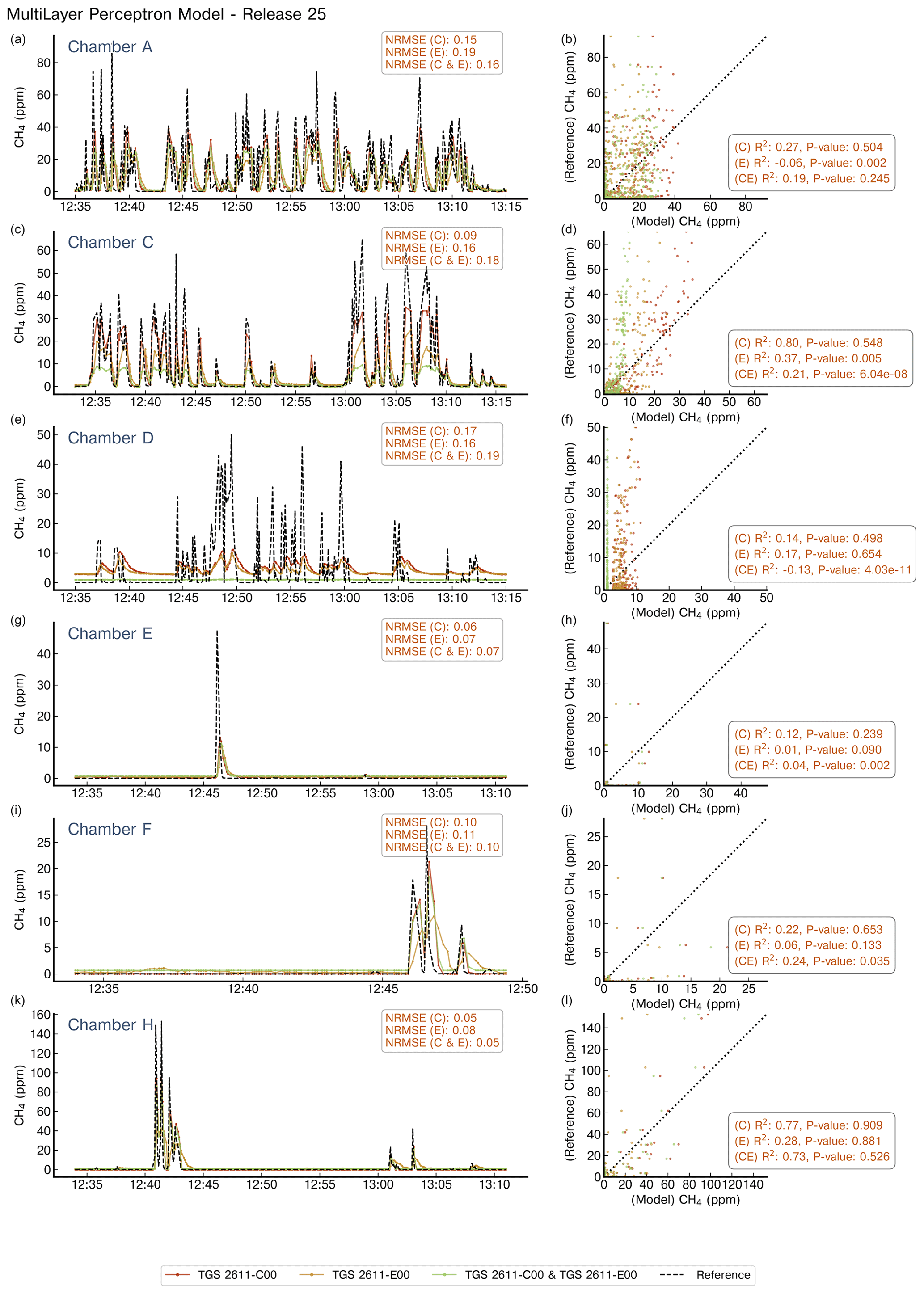
Figure 5Example of reconstruction of release no. 25 using a MLP model. The left panels show the reconstructed CH4 mole fractions for each chamber that captured the release; we present the reference signal (black dotted line), the reconstructed CH4 mole fractions when the model has as input the TGS 2611-C00 sensor (red), the TGS 2611-E00 (yellow), or both types at the same time (green). The right panels show the 1 : 1 plot of the reference against the output of the model for the three configurations of inputs. Note the difference in the x axis for chamber F.
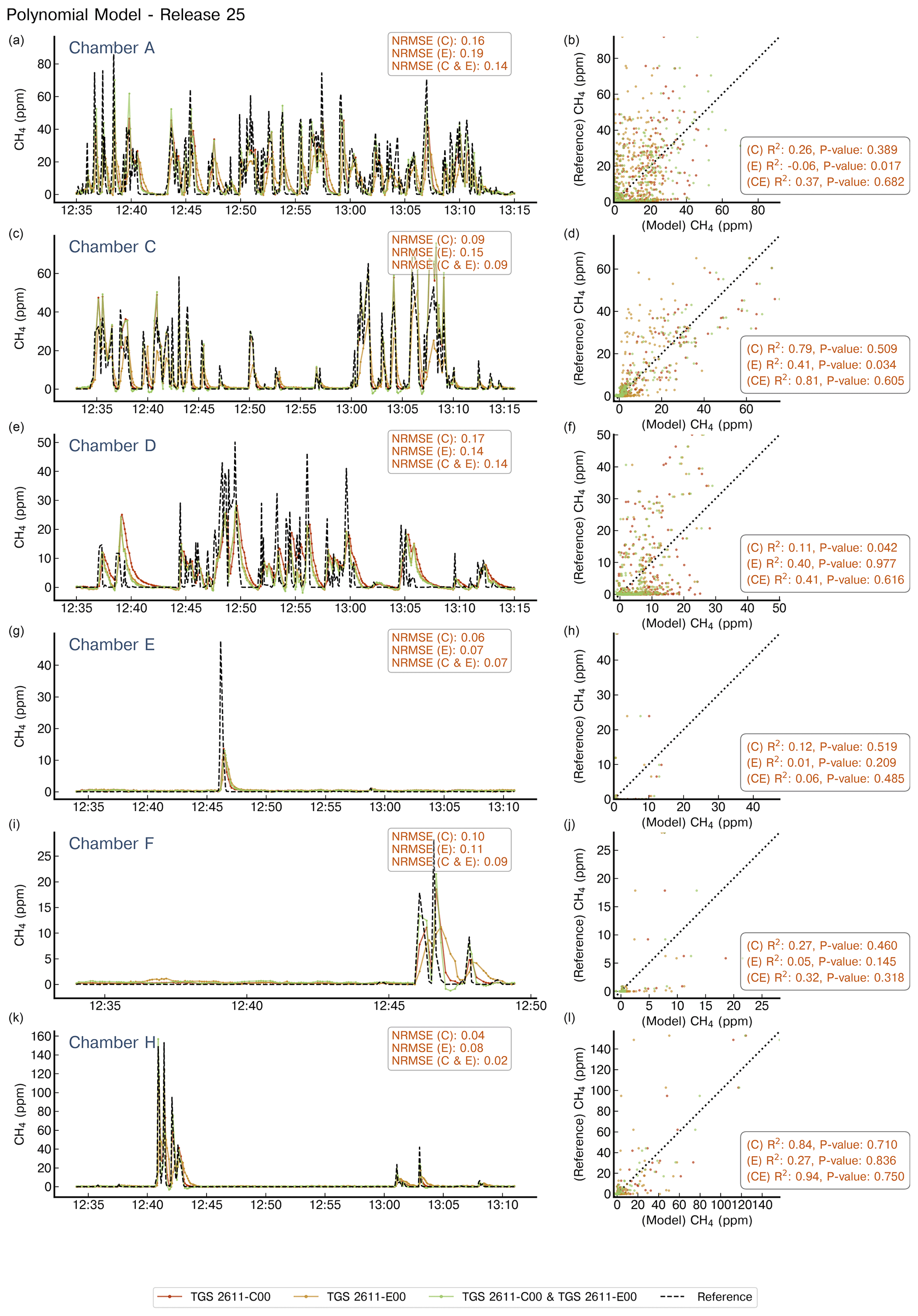
Figure 6Example of reconstruction of release no. 25 using a polynomial model. Notations are the same as in Fig. 5.
We found that both the MLP and second-degree polynomial models had similar performance across the releases, regardless of the chamber used for CH4 mole fraction reconstruction. For two releases sampled by chamber A (releases no. 10 and 26; see Figs. A6 and A9 for MLP model and Figs. A11 and A12 for the polynomial model, respectively), characterised by amplitudes below 10 ppm, the polynomial model provides a noisy signal as output regardless of the configuration of the inputs used. There were, however, some cases in which the polynomial model outperformed the MLP, for example, the four releases sampled by chamber D, where the MLP model produced a systematic underestimation of the reconstructed CH4 mole fraction on the three configurations of inputs.
Regarding the two TGS types tested in this work, the type C sensor used alone produced better reconstructions than the type E sensor alone, as well as both types used as simultaneous model input. Type E sensors showed phasing errors in the form of a slow decay after large spikes and uncorrelated spikes not detected by the reference gas analysers, for example, during release no. 9 from chamber D (Figs. A5 and A10 for the MLP and the polynomial model, respectively). Simultaneous use of both sensors (type C and E) as model input produced outputs closer to model outputs trained with only type C sensor data. MLP models also presented, for some releases, a saturation of the outputs (releases no. 9, 12, and 25 for chamber D (Figs. A5, A7, and 5) and release no. 21 for chamber H (Fig. A8)) or a systematic bias (releases no. 2, 10, and 26; see Figs. A4, A6, and A9). For releases with peak amplitudes above 40 ppm, a systematic underestimation is observed regardless of the reconstruction model or the sensor type used as input.
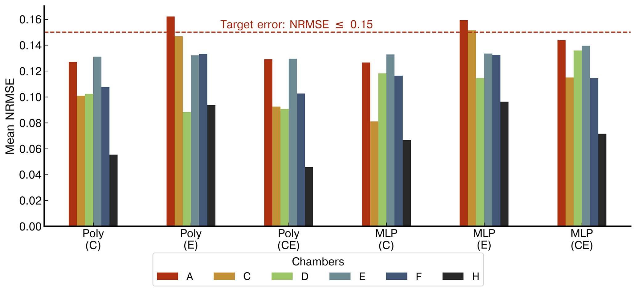
Figure 7Comparison of the mean NRMSE of the two types of models trained with the three configurations of the inputs. The second-degree polynomials are denoted as “Poly” and the multilayer perceptron as “MLP”. The three input configurations are denoted inside parentheses: “C” when the model's input was only the TGS 2611-C00, “E” for the TGS 2611-E00, and “CE” when both sensors were used as inputs at the same time. The colour code of the bars corresponds to the chambers.
Figure 7 summarises the performance of the reconstruction on the testing data set using the NRMSE error defined in Eq. (1). All chambers reached our target error (NRMSE ≤ 0.15), except in three cases corresponding to models using the type E sensor as input (chamber A for polynomial model and MLP and chamber C for MLP). Imposing a stricter target requirement of NRMSE ≤ 0.1, only chamber H satisfied the target error regardless of the reconstruction model or the sensor used. Performance is similar when using the type C sensor as model input regardless of the choice of model across all the chambers. When using both sensor types at the same time as model input, the second-degree polynomial provides better reconstruction than the MLP model, especially for chambers C, D, and H (NRMSE = 0.09, 0.09, and 0.04 for the polynomial model and 0.11, 0.13, and 0.07 for the MLP). Chamber D, characterised by having limited training data, produced a systematic lower error when using the polynomial model than when using the MLP model, regardless of the input variable used.
In summary, the model used in the reconstruction is important only for cases where there is limited information available for model training. We also conclude that type C sensors alone produced a better reconstruction of CH4 spikes than either using type E sensors alone or using both types of sensors as model input.
3.2 Release rate and location estimates based on the observations from the TGS sensors
Average CH4 mole fraction enhancements above the background and of their spatial gradients are displayed for release no. 25 in Fig. 8. This figure compares the values of reconstructions from the low-cost sensors using the MLP model (see Fig. A13 for the values corresponding to the polynomial model), with corresponding measurements made by the high-precision gas analyser. It also shows simulations resulting from inversions assimilating either the reference high-precision data or reconstructed TGS data. Since the best reconstruction performance was obtained when using the type C sensor, the inversion results presented here are based on reconstructions from only this type of sensor. For release no. 25, used as an example here, the procedure to define average values per wind sectors resulted in four bins, with an approximate size of 10°. To simplify the numbering when mentioning the reference instrument or the TGS, we refer to the chamber identifier X (REF-X and TGS-X, respectively, with X the name of the chamber). The contour plot of the cost function is presented in Fig. A15, showing the controlled release location and the inversion estimated location when assimilating TGS data.
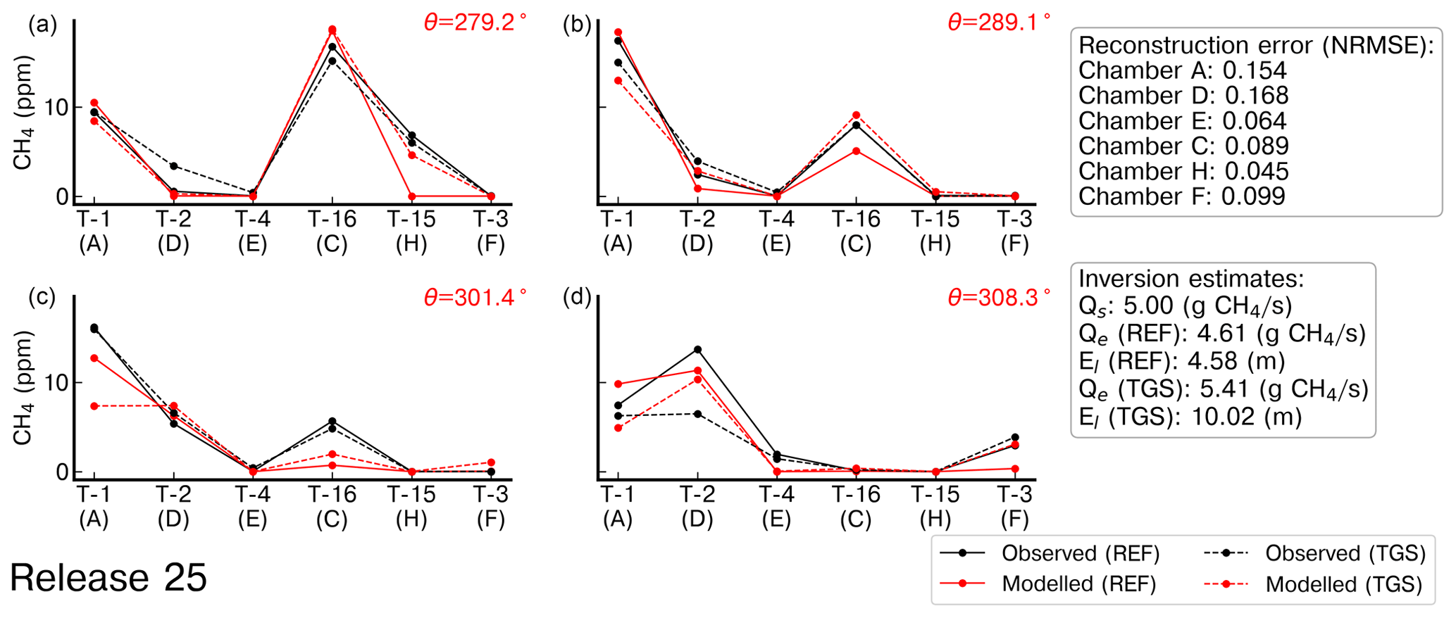
Figure 8Observed and modelled average CH4 mole fractions from the reference gas analyser, denoted as “REF”, and TGS 2611-C00 sensors, denoted as “TGS”, corresponding to release no. 25. Reconstructed CH4 measurements were computed using the MLP model. The index of the air inlets is denoted as T-x, and the average wind direction (θ) for the binning of wind sectors is shown on the top right of each panel in red.
In general, the observed spatial CH4 mole fraction gradients between the different stations are similar when considering the reference gas analyser measurements and the reconstructed CH4 mole fractions from the TGS, except for few cases where the reference is better, for example, for release no. 25 (see Fig. 8). During release no. 25, observed gradients from TGS-D data underestimate the actual gradients given by REF-D for θ = 308.3° and overestimate them for θ = 279.2°, where θ is the average direction of the wind sector.
The modelled average mole fraction enhancements and thus the modelled gradients assimilating reference data are very close, in general, to the ones from these reference data, although some discrepancies can occur, for example, for release no. 25, for REF-H with θ = 279.2°, REF-C with θ = 301.4° and θ = 289.1°, and REF-A with θ = 301.4 and 308.3°. For most of the cases, the modelled gradients assimilating the TGS data are closer to those assimilating the reference data than to the observed TGS data. In addition, the observed TGS data, for some cases, is closer to the observed reference one than to the modelled gradients assimilating either reference or TGS data, highlighting the higher impact of the model error on the inversion than the reconstruction error of CH4 mole fractions.
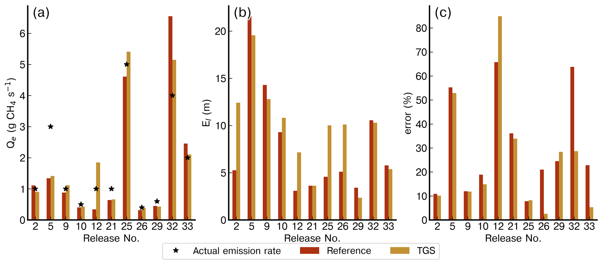
Figure 9Comparison of the emission rate estimate (Qe) (a), of the location error (El) (b), and of the relative error in the emission rate estimate (c) from the inversions assimilating the reference data (in red) and the reconstruction of the CH4 mole fraction from the TGS sensors (in orange). The reconstructed CH4 mole fractions used in these inversions are computed with the MLP model.
Figure 9 shows a comparison of emission rate estimates with corresponding relative error in the estimation of emission rate and location error across the 11 releases of the testing data set. This figure shows estimates assimilating CH4 mole fractions from the TGS using reconstructions from the MLP model (see Fig. A14 for results when assimilating reconstructed mole fraction measurements based on the second-degree polynomial model).
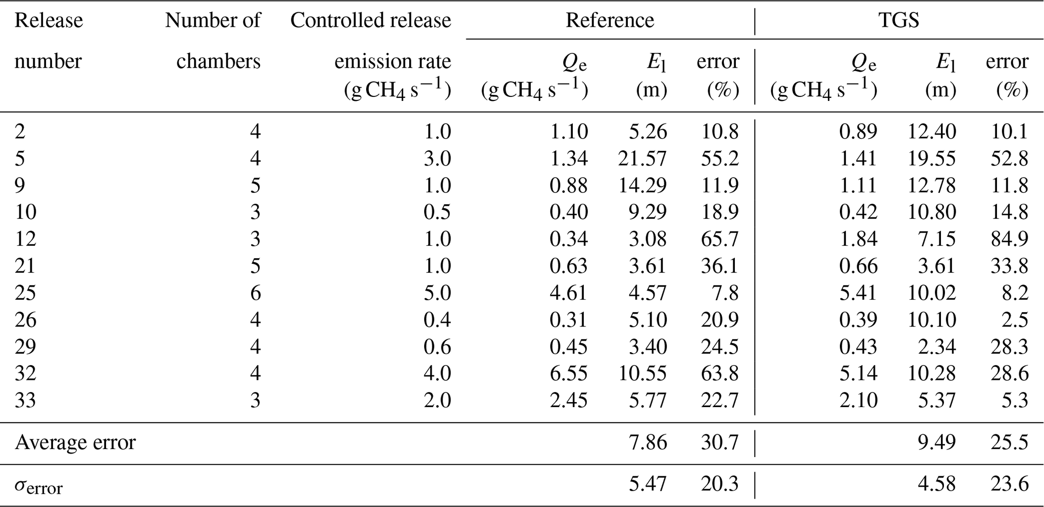
Regarding the release rate estimates, those from inversions assimilating the reference mole fractions bear an average error of 30 %, and those from the inversion assimilating data from the TGS sensors bear an average error of 25 %. In the case of the estimation of the release location, the assimilation of the reference data produces a slightly smaller average localisation error of 7.86 m (σ = 5.47 m) compared to 9.49 m (σ = 4.58 m) from the assimilation of TGS data. For five releases (no. 2, 10, 12, 25, and 26), the assimilation of reference data yields a better estimate of the location, and for one release (no. 21), both inversions yield similar localisation errors.
In general, emission rate estimates (see Fig. 9a) derived using CH4 mole fraction from reference gas analyser and reconstructed from TGS data are similar. For three releases (no. 12, 25, and 32), we observe large errors in the release rate estimate. Inversion assimilating reconstructed TGS data or reference gas analyser mole fraction measurements highly underestimate the rate for release no. 5 (1.41 and 1.34 g CH4 s−1, respectively, with a controlled release rate of 3.0 g CH4 s−1) and strongly overestimate the rate for release no. 32 (5.14 and 6.55 g CH4 s−1, respectively, with a controlled release emission rate of 4.0 g CH4 s−1). Modelling using measurements from the reference gas analyser provides a slightly better estimation of release locations than the using reconstructed TGS data. Only for releases no. 29 and 33 does the inversion assimilating reconstructed TGS data provide slightly better source localisation. Conversely, for releases no. 2, 12, 25, and 26, the location error from the inversion assimilating reconstructed TGS data is almost double that derived using reference gas analyser measurements. The errors on the emission rate estimate from both inversions was smaller than 30 % for most of the releases, except for four cases, where errors reached 80 % for the inversion assimilating reconstructed TGS data and 65 % for the inversion assimilating reference gas analyser measurements, respectively. There were two cases, releases no. 26 and 33, when the inversion assimilating reconstructed TGS measurements produced a much lower error (2.5 % and 5.3 %, respectively) in the emission flux quantification than the inversion assimilating reference gas analyser observations (20.9 % and 22.7 %, respectively). The fact that the assimilation of the TGS reconstructed CH4 data can yield better results than when using accurate CH4 mole fraction measurements made by the reference instrument highlights the impact of the transport model error (associated with the simulation of the average mole fractions with the Gaussian model) in the inversion process. These errors dominate the resulting errors in the estimates of the release rate and location when assimilating the reference data (Kumar et al., 2022). They appear to have a weight larger than that of errors in reconstructed mole fraction from TGS data when assimilating these data.
Baseline voltage correction of TGS sensors, in this study, assumes that the targeted voltage signal measured by the sensors corresponds to a series of high-frequency spikes produced as a result of the emission plume intermittently intersecting the various sensor air inlets, due to atmospheric turbulence and high-frequency wind variations. Our approach of deriving a baseline voltage signal offers a suitable alternative to otherwise correct the TGS observations when little or insufficient information is available to derive an analytical baseline voltage correction model (e.g. from measurements of H2O mole fraction and temperature). This approach is interesting for conditions when environmental parameters are highly variable or baseline voltage correction models do not dispose of sufficient observations to derive robust relationships to correct for the effects of environmental variables on TGS baseline voltage signal. This case corresponds well with the measurements presented in this study. However, in some cases, the plume can intersect the sensor air inlet for a prolonged duration, resulting in a voltage signal not only exhibiting high-frequency spikes but also resulting in continuously varying voltage enhancements above the baseline voltage level. For those cases, our baseline voltage method would not be able to distinguish the sensor voltage enhancements corresponding to the CH4 mole fraction enhancements due to the plume as opposed to the atmospheric background; we would then need to reconsider the option of deriving a voltage baseline based on environmental parameters (H2O mole fraction and T).
Regarding the type of TGS used in CH4 mole fraction reconstruction, we obtain best performance (compared to the reference gas analyser) using only type C sensors as model input. The fast decay observed for reconstructed CH4 mole fraction measurements after each voltage spike was attributed to the response time of the TGS sensor. The slow decay observed on type E sensors was probably due to a filter integrated inside the sensor causing the improvement of CH4 selectivity. Concerning the reconstruction models, the polynomial and the MLP models produced similar results with few differences. This confirms our previous study (Rivera Martinez et al., 2023a), where we observed that the performance of CH4 mole fraction reconstruction models was mainly driven by the type of used sensor rather than the choice of reconstruction model. In cases with a low information content (i.e. only few observed voltage spikes, limited voltage range, and variability of the spike magnitude, frequency, and duration) in the training data set (e.g. when reconstructing CH4 mole fraction for chamber D), the second-degree polynomial model provides more accurate mole fraction estimates than the MLP model. This is probably due to data distribution within the training data set used by the MLP model to compute its parameters, not representing the same range of variations within the testing data set. For spikes with mole fraction enhancements of under 5 ppm, the MLP model with the type C sensor signal as input produced a more accurate reconstruction than either using the type E sensor alone or using both sensor types simultaneously as model inputs. The combination of both sensors as input produced a reconstruction of CH4 mole fractions similar to using only one of the sensors (TGS 2611-C00). This can be explained by the fact that both of the TGS signals are highly correlated and do not add more information to the model, as well as the phase mismatch between both input signals produced by the filter on the TGS 2611-E00 sensor. The noise in the voltage signal during some releases, for example, release no. 26 on chamber A, was not correctly removed during the polynomial model mole fraction reconstruction. However, for the type C sensor, the MLP model reduces the voltage signal noise, resulting in a more accurate mole fraction reconstruction.
Regarding the inversion of emission rates and locations using the Gaussian plume model framework developed by Kumar et al. (2022), we obtained good estimates and performance with the reconstructed time series of CH4 mole fraction spikes from voltage measurements of TGS sensors, and the results are comparable to those obtained when assimilating corresponding mole fraction measurements from the reference gas analyser. We observed that the simulated gradients of the Gaussian model assimilating observations from the TGS chambers were close to simulated gradients of the reference inversions (assimilating measurements from the high-precision gas analyser), even if the observed gradients were sometimes in a different direction. In most cases errors from both inversions ranged between 2.5 % and 55 % except for releases no. 12 and 32, where the error reached 65 % and 63 % for simulated gradients assimilating the reference data, respectively, and release no. 12, with an 85 % error for simulated gradients assimilating the TGS data. The overall inversion performance assimilating TGS data and reference data is good and consistent. The slightly better average performance in the release rate estimates using TGS data (25 % error) than using reference data (30 % error) is not significant with regards to the overall variability of the results and highlights the weight of the model errors associated with the simulation of the average mole fraction with a Gaussian model. These results demonstrate that the errors in the release rate and location estimations from inversions using both reference and TGS data are dominated by model errors in the inversion framework. The errors in the reconstruction of the CH4 mole fraction spikes from the TGS voltage data are thus sufficiently low for use in the inverse modelling problem analysed here.
One should note that, as mentioned on Sect. 2.7, in this study, reference inversions rely on a restrained subset of the reference data that match the available data from TGS sensors. Results from Kumar et al. (2022) considering the full reference data set yielded significantly superior results.
4.1 Detection threshold and differentiation of emission types
Our methodology requires for emissions to be sustained for long enough to be captured within each sampling interval. The principal limitation of our method is the requirement for at least four 1 min averages, restraining the detection of short-lived emissions. Another challenge lies in the detection of emission types, such as vented, combustion, or fugitive emissions. This aspect, which is out of the scope of our study, would require a detailed study of the characteristics of each kind of emission, requiring additional tools to distinguish their individual particularities.
4.2 Limitations of the inversion framework
The inversion approach applied here, described for a single emission source only as required by the controlled release experiments, can be easily extended to estimate emissions from multiple sources (see Singh et al., 2013). However, estimating emissions from multiple sources may require a denser network of sensors to constrain a larger number of parameters for all sources. However, significant uncertainties may arise in emission estimates when measurements are taken in very close proximity to the emission sources. Our methodology requires that emissions be sustained long enough to be captured within the sampling intervals. The principal limitation is the requirement for at least four 1 min averages, restraining the detection of short-lived emissions. Another challenge lies in the detection of emission types, such as vented, combustion, or fugitive emissions. This aspect, which is out of the scope of our study, would require a detailed study of the characteristics of each kind of emission, requiring additional tools to distinguish the particularities of them.
4.3 Density of sensor network
In our campaign, we deployed seven chambers connected to air inlets placed on tripods at distances of between 40 and 50 m from the emission source to capture methane plumes under various conditions. Table 3 details the number of sensors used for emission flux estimations across the controlled releases. The optimal number of sensors for emission flux localisation and estimation is complex and is influenced by varying emission rates, environmental conditions, and setup configurations. Notably, when examining cases with uniform emission rates (1 g CH4 s−1), such as releases no. 12, 2, and 21 (with three, four, and five chambers, respectively), a configuration of four to five sensors consistently produced the lowest errors for both sensor types. Yet, release no. 21 demonstrated that even five sensors may not guarantee low errors if the plume capture is suboptimal due to environmental factors or sensor placement.
Table 3Comparison of the emission rate estimate (Qe), location error (El), and relative error of flux rate estimates for inversions assimilating reference gas analyser measurements and reconstructed TGS mole fractions using the MLP model.
We can contrast our setup with Riddick et al. (2022), who used four sensors approximately 30 m away from the source, but without detailing their individual contributions to emission calculations. The optimal configuration of such a relatively dense network necessitates a thorough investigation, possibly through simulations of typical emissions and the strategic addition or removal of sensors to assess their impact. However, a comprehensive analysis of optimal network configuration was beyond the scope of our study due to the limited number of data points recorded.
4.4 Computational efficiency of the inversion framework
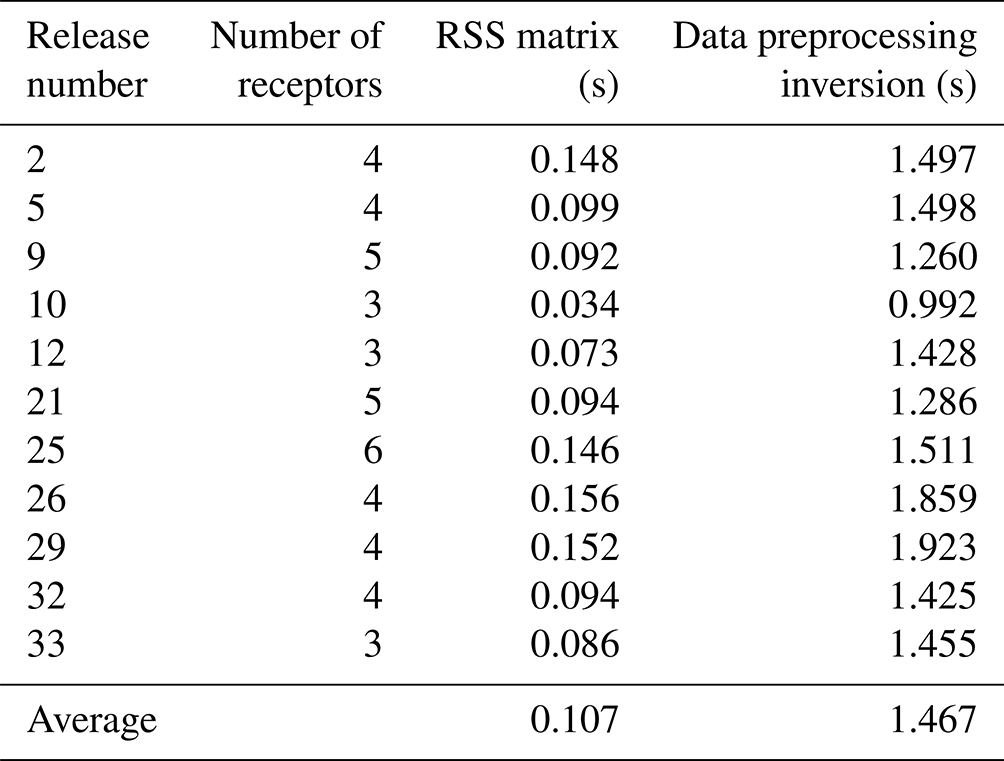
Our inversion framework, developed in Python 3.8 utilising NumPy, pandas, and SciPy libraries, efficiently computes the RSS matrix through vectorised operations and a nested for loop. This approach achieves an average computation time per release of 0.1 s for the RSS matrix and 1.46 s for full code execution, including data preprocessing on an eight-core Apple Silicon M1 processor. The framework, which can be further optimised with multiprocessing, is detailed in Table A7, showcasing computational times across different releases. It effectively estimates emission rates and source locations on a fine grid (40 m × 50 m × 8 m, discretised at 1 m × 1 m × 0.5 m), demonstrating practicality for real-world applications at minimal computational costs.
While our work presents promising results regarding the use of low-cost MOS sensors for estimating CH4 emission rates and locations, it is imperative to acknowledge the high degree of uncertainty associated with continuous emission monitoring (CM) solutions, as evidenced by the study conducted by Bell et al. (2023). In their study, various CM technologies were tested against a series of controlled releases, revealing a broad range of true-positive rates, false-positive rates, and significant errors in the estimation of emission rates. Bell et al. found considerable variability in the performance of CM technologies, with mean relative errors (MREs) ranging from −44 % to +586 % for release rates of between 0.1 and 1 kg h−1 and MREs ranging between −40 % and +93 % for release rates above 1 kg h−1. These findings underscore the current limitations and inconsistent performance of CM solutions, even under less complex conditions than typically encountered in the field. While our study is encouraging, it represents just one step in the progression of this approach.
Our study demonstrated the capability of metal oxide sensors to be used with flux algorithms to estimate emission rate and location during a controlled CH4 release experiment, with release rates typical of those expected from gas leaks from industrial facilities. Our TGS voltage baseline correction algorithm allowed us to identify TGS voltage variations related to the high-frequency variation of the plume across the different sensor inlets. We compared the performance of two models, second-degree polynomials and MLP, to reconstruct CH4 mole fractions from voltage drop measurements during the controlled releases for three configurations of data from TGS units as inputs for the reconstruction algorithm. The reconstructed CH4 mole fractions were used as input to an inversion modelling framework for emission localisation and flux quantification for each release not otherwise used for model training (i.e. the testing data subset). Results of inversions assimilating reconstructed TGS mole fraction were compared with those assimilating corresponding reference (CRDS) mole fraction measurements.
The reconstruction of CH4 mole fraction from voltage measurements made during controlled releases showed good agreement with corresponding measurements made by high-precision reference gas analysers. The reconstruction was consistently better using data from the TGS 2611-C00 regardless of the reconstruction model used. Both CH4 mole fraction reconstruction models satisfied our targeted NRMSE requirement of lower than 0.15 for all chambers, when trained with the TGS 2611-C00. Emission rate and source location estimates using an inversion based on a Gaussian plume model produced similar results using reconstructed CH4 mole fraction derived from TGS sensors to those obtained using high-precision measurements, with an average estimated TGS emission rate error of 25.5 % and a mean source location error of 9.5 m. In this study, the reconstruction of the CH4 mole fractions was conducted independently of inversion modelling. The emission flux estimation error could probably be reduced with a better understanding of inverse modelling sensitivity to the misfits from the reconstruction models. In consequence, a sensitivity study is encouraged in future to determine the best approach for the reconstruction TGS-derived methane mole fraction.
Second-degree polynomials proven to be robust to derive relationships between TGS voltage signal related to spikes and CH4 mole fraction (Rivera Martinez et al., 2023a) are defined by
where is the predicted CH4 concentration and x1 is the corrected voltage of the TGS after removing the effects of the baseline.
Artificial neural networks have been widely used to derive non-linear relationships between predictors and independent variables in many applications, as a universal approximator method (Hornik et al., 1989), and for their generalisation capabilities (Haykin, 1998). In previous studies (Casey et al., 2019; Eugster et al., 2020; Rivera Martinez et al., 2021, 2023a), ANNs were employed to derive CH4 mole fractions from TGS observations on different sampling configurations (field and laboratory conditions) with good agreement between the reference observations and the outputs produced from the models. The simplest architecture of an ANN is the multi-layer perceptron (MLP), consisting of a series of units (neurons) in fully connected layers. The inputs of any unit will be the weighted sum of the outputs of the previous layer, to which an activation function (ReLU, tanh, etc.) is applied. As a supervised machine learning approach, it requires a training basis to learn the relationships, adjusting the weights of its connections, between the inputs and outputs using an iterative process known as optimisation. The problems of MLP models are either the underfit of data; the production of a high error on the train set which can be mitigated with a sufficiently large network; or overfitting, which produces a high test error when they cannot generalise to new examples. Regularisation terms and early stopping techniques are helpful to prevent overfitting (Bishop, 1995; Goodfellow et al., 2016). Here, we have trained the MLP model using the Adam optimiser (Kingma and Ba, 2014; Géron, 2019), and the optimal number of units and layers was determined using a grid search technique (Géron, 2019), resulting in 50, 10, and 5 units per layer with ReLU as the activation function for the hidden units. A regularisation factor of α = 0.05 and early stopping was used to prevent overfitting.
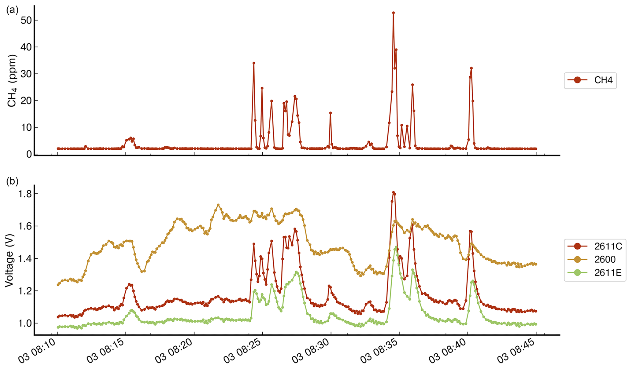
Figure A1Comparison of the voltage measurements from three types of TGS included on chamber A. Panel (a) shows the reference CH4 observations measured from the reference instrument. Panel (b) shows the voltage observations from TGS 2611-C00, 2600, and 2611-E00.
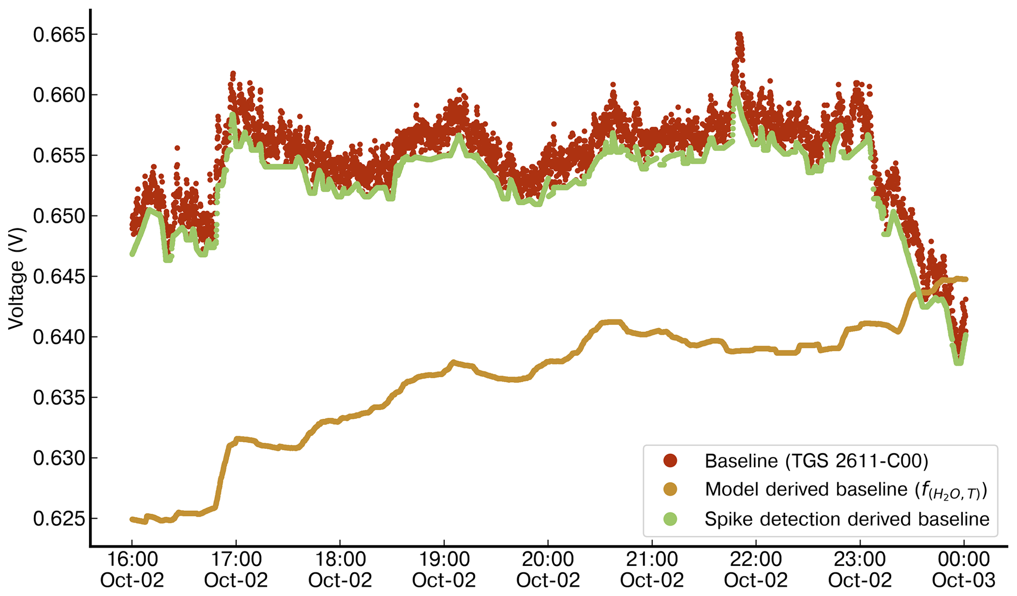
Figure A2Comparison of the performance in deriving a baseline signal for the TGS 2611-C00 (red) of chamber E between a function of H2O and temperature (yellow) and a spike detection algorithm (green). The multilinear-model-derived baseline was trained on 6 h of non-release periods at the start of the first day of the campaign and evaluated on the last 8 h of the same day (shown in the figure). The spike detection algorithm, an iterative function, does not need any prior training and detects the baseline based on neighbouring observations and fixed parameters.
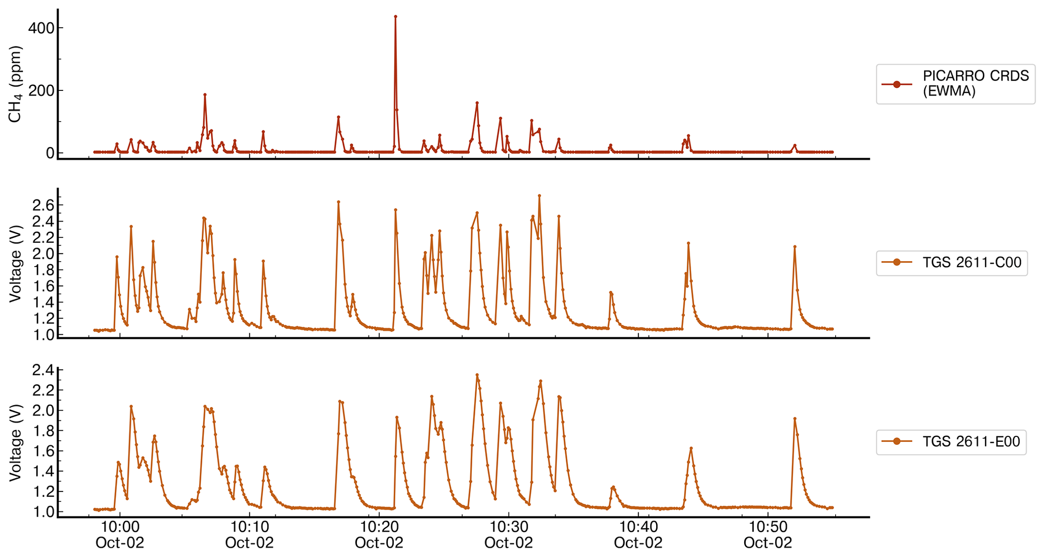
Figure A3Comparison of the response of the TGS 2611-C00 and TGS 2611-E00 sensors with CH4 measurements from the reference instrument for release no. 2, which contains spikes with high concentration. The spikes observed on the TGS sensors corresponding to amplitudes from 100 ppm to more than 200 ppm are not distinguishable from spikes with amplitudes lower than 50 ppm.
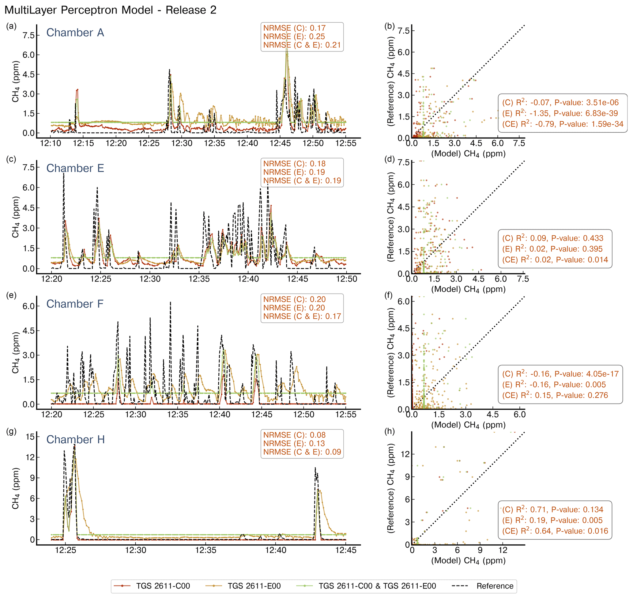
Figure A4Reconstruction of release no. 2 using a MLP model. The left panels show the reconstructed CH4 mole fractions for each chamber that captured the release; we present the reference signal (black dotted line), the reconstructed CH4 mole fractions when the model has as input the TGS 2611-C00 sensor (red), the TGS 2611-E00 (yellow), or both types at the same time (green). The right panels show the 1 : 1 plot of the reference against the output of the model for the three configurations of inputs. Note the difference in the x axis for the chambers.
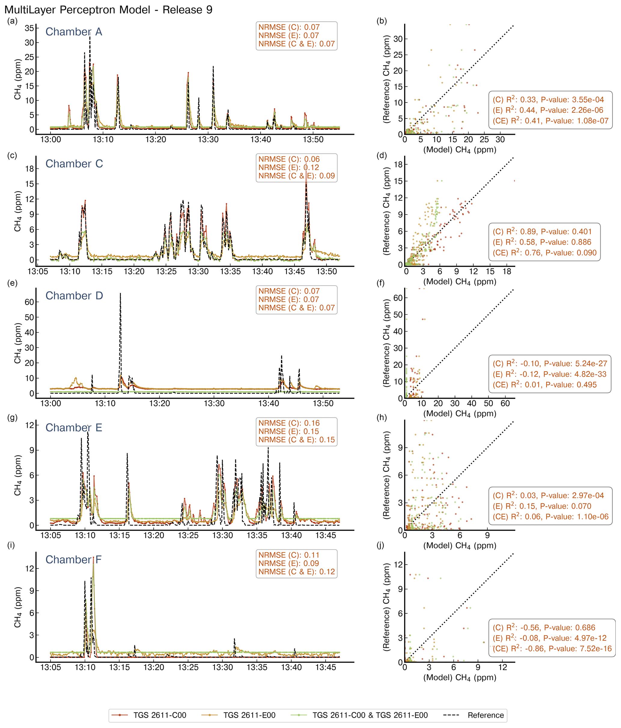
Figure A5Reconstruction of release no. 9 using a MLP model. Notations are the same as in Fig. A4. Note the difference in the x axis for the chambers.
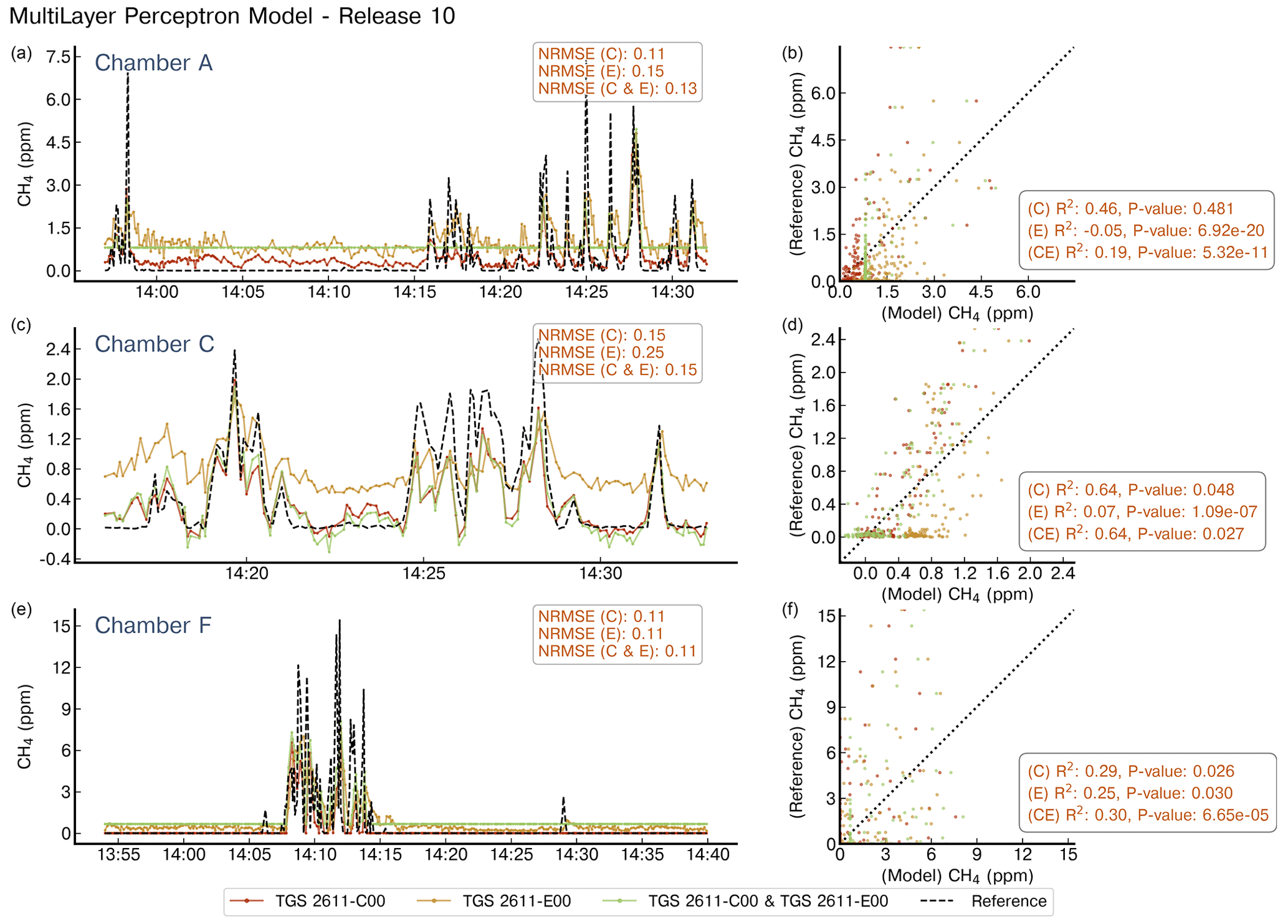
Figure A6Reconstruction of release no. 10 using a MLP model. Notations are the same as in Fig. A4. Note the difference in the x axis for the chambers.
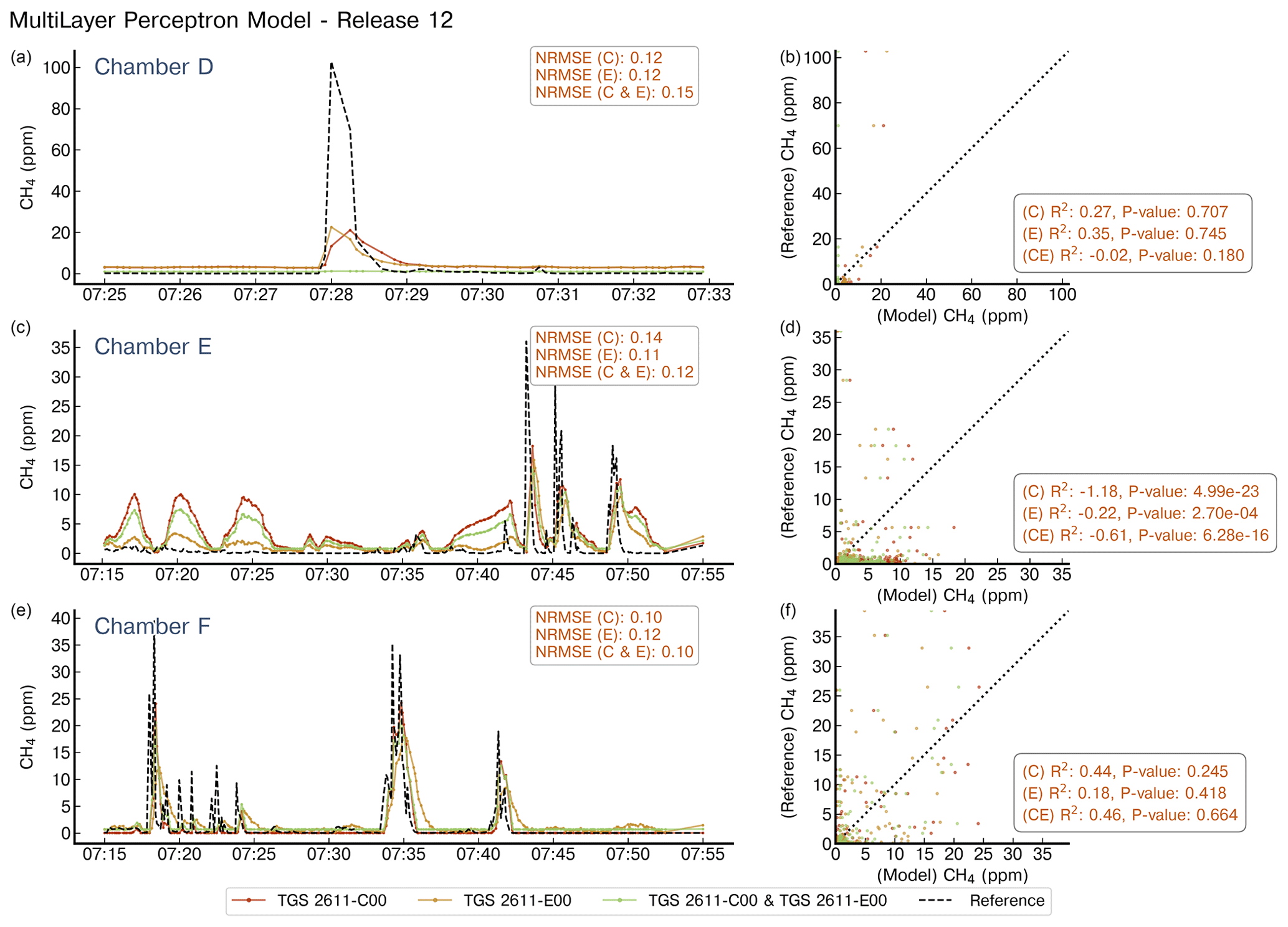
Figure A7Reconstruction of release no. 12 using a MLP model. Notations are the same as in Fig. A4. Note the difference in the x axis for the chambers.
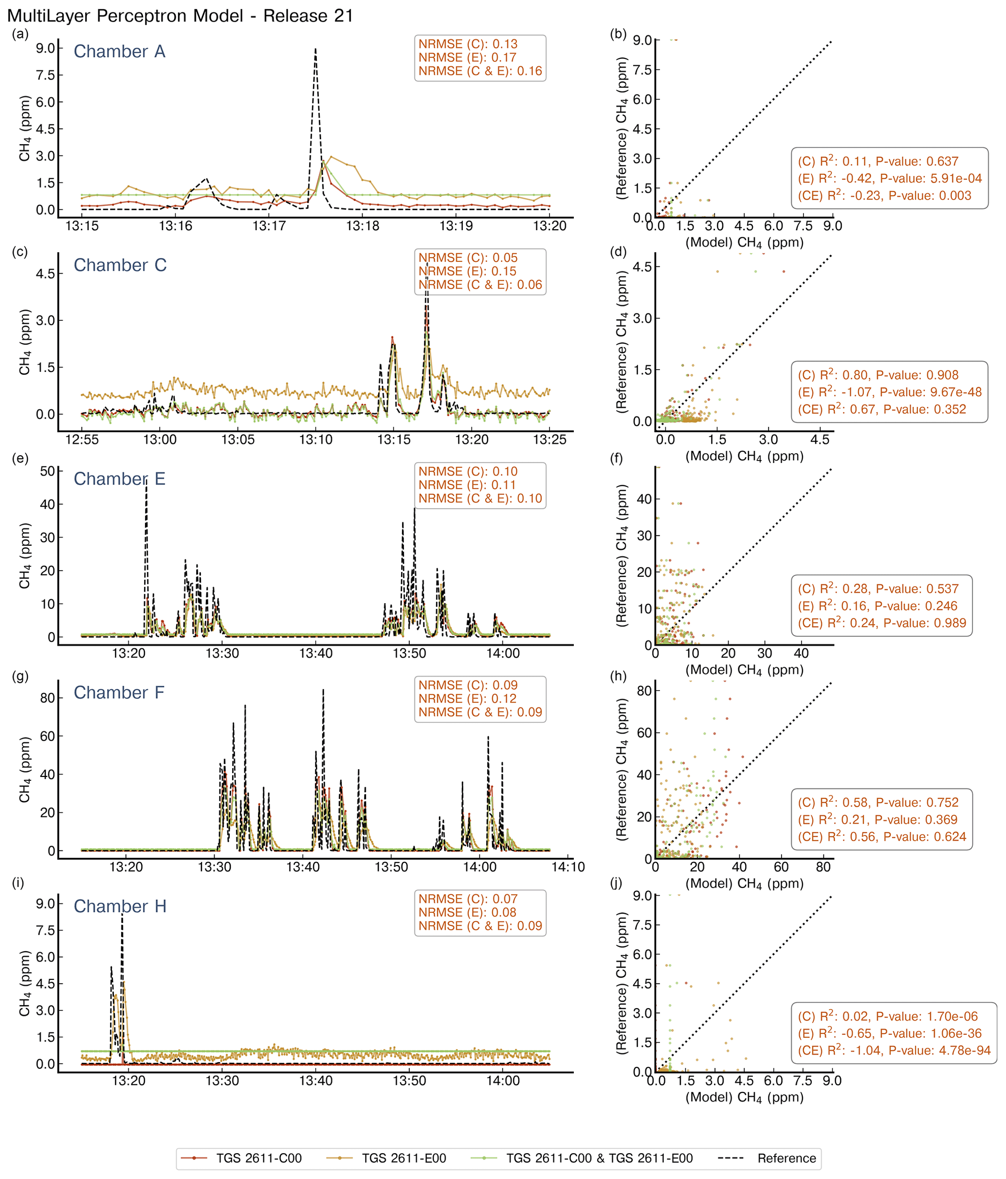
Figure A8Reconstruction of release no. 21 using a MLP model. Notations are the same as in Fig. A4. Note the difference in the x axis for the chambers.
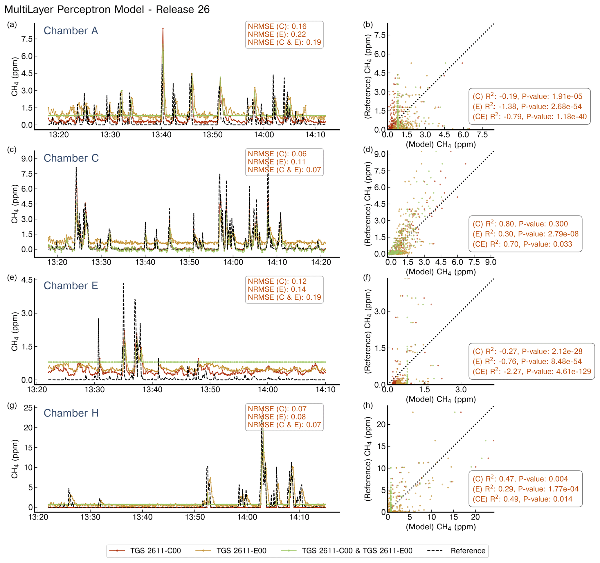
Figure A9Reconstruction of release no. 26 using a MLP model. Notations are the same as in Fig. A4. Note the difference in the x axis for the chambers.
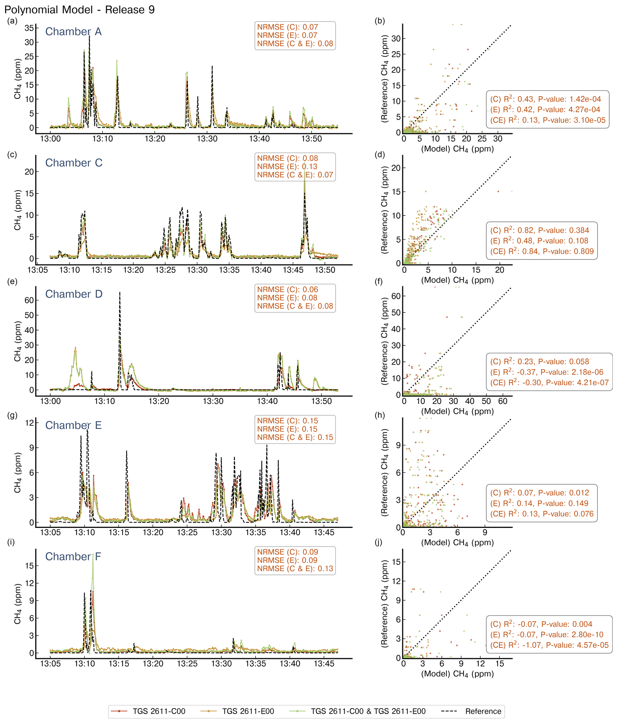
Figure A10Reconstruction of release no. 9 using second-degree polynomials. Notations are the same as in Fig. A4. Note the difference in the x axis for the chambers.
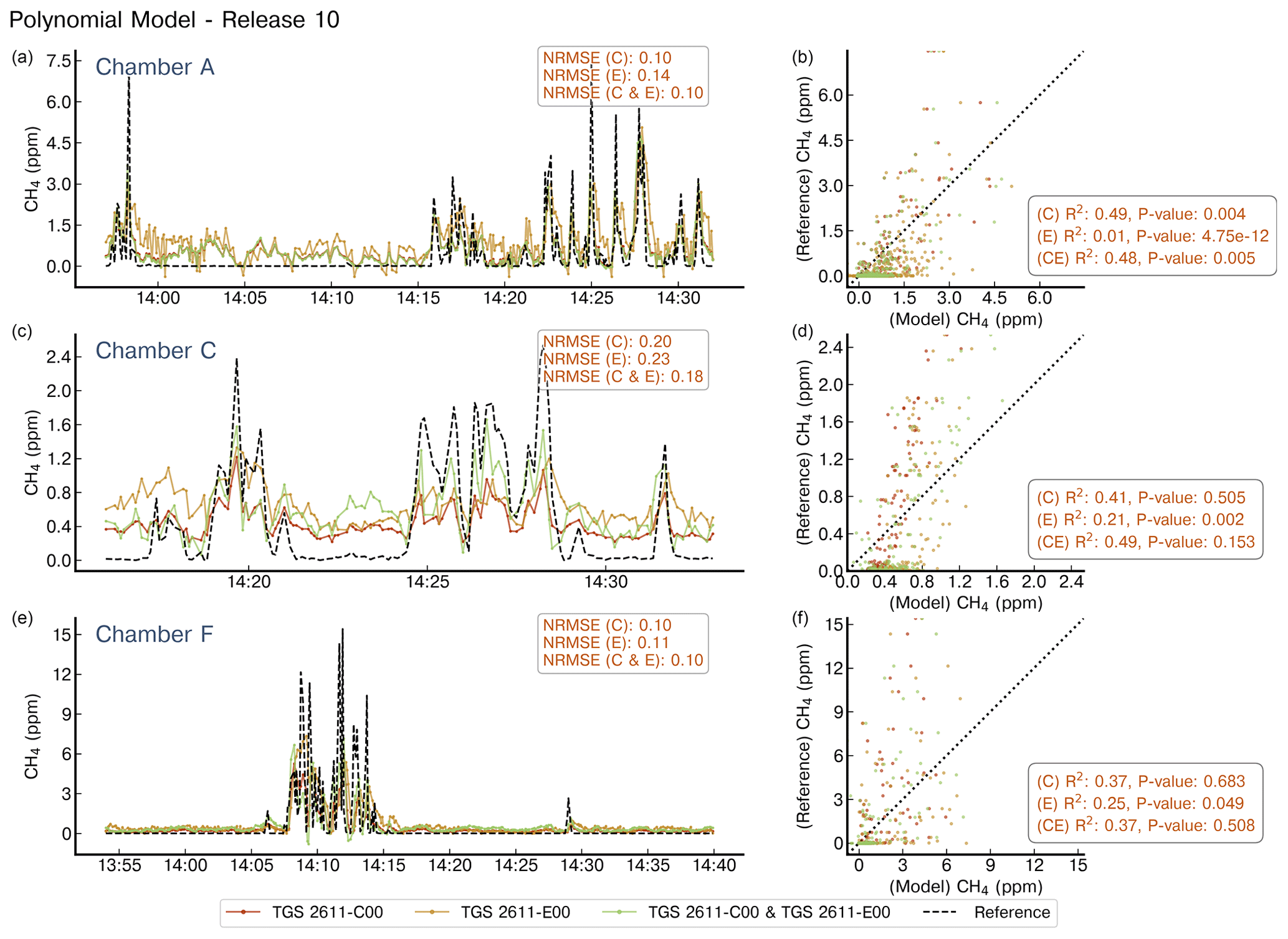
Figure A11Reconstruction of release no. 10 using second-degree polynomials. Notations are the same as in Fig. A4. Note the difference in the x axis for the chambers.
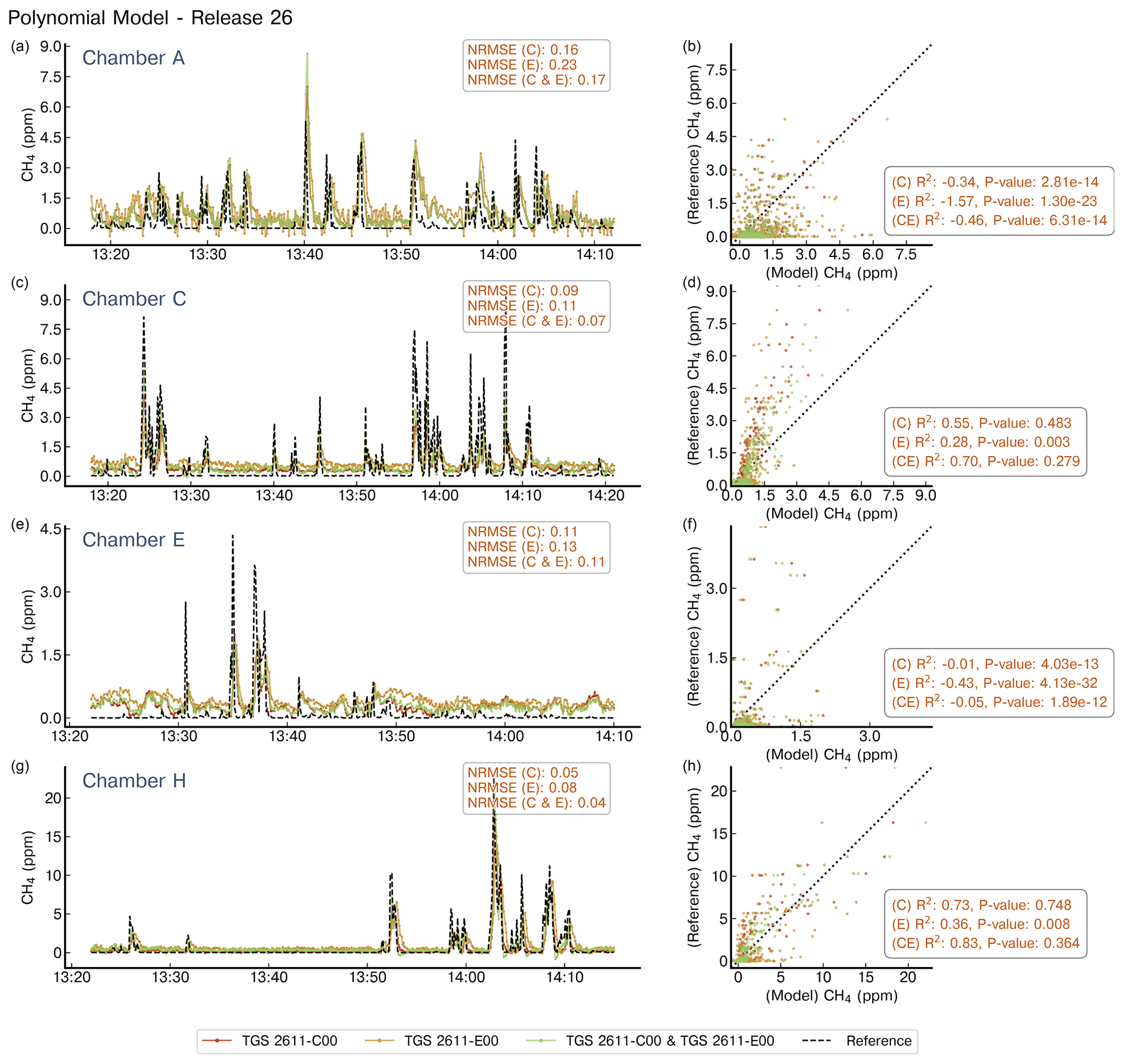
Figure A12Reconstruction of release no. 26 using second-degree polynomials. Notations are the same as in Fig. A4. Note the difference in the x axis for the chambers.
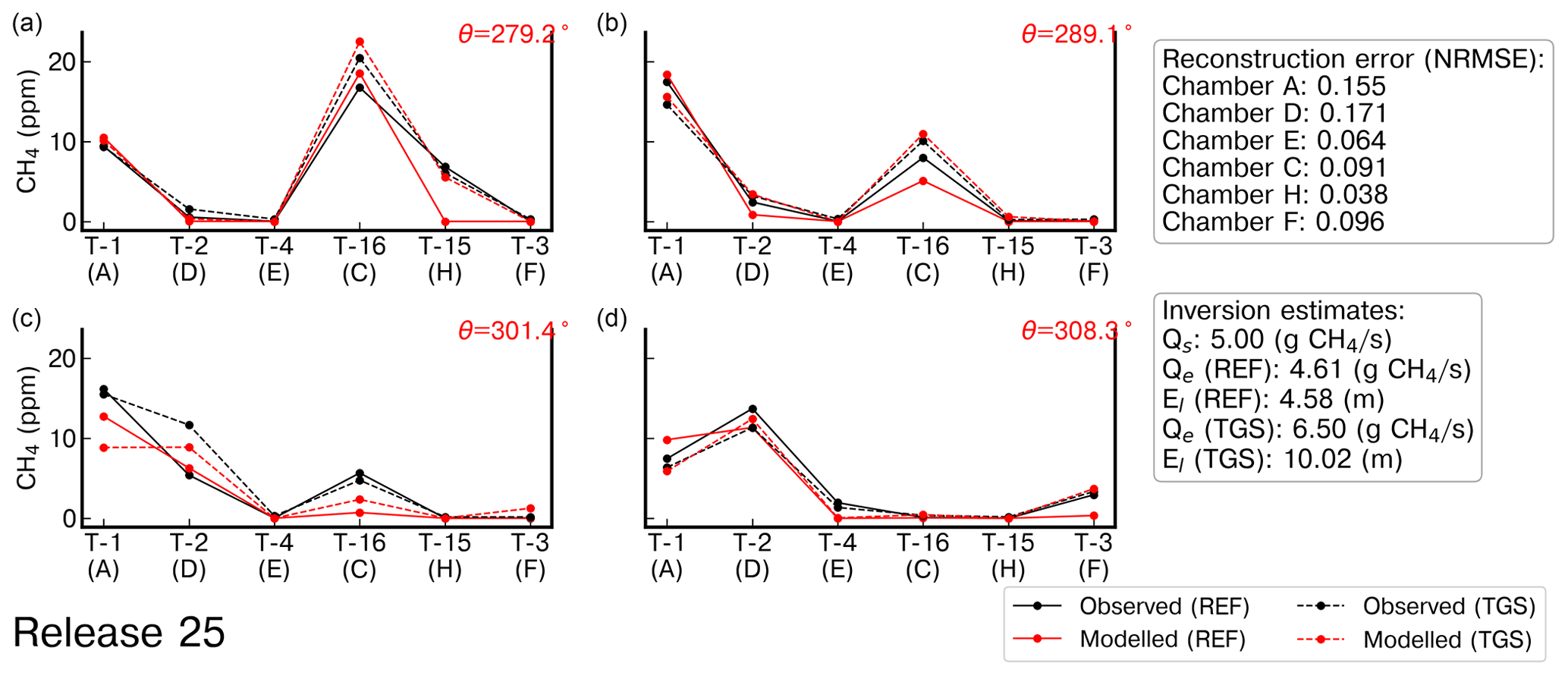
Figure A13Observed and modelled average CH4 mole fractions from the reference gas analyser, denoted as “REF”, and TGS 2611-C00 sensors, denoted as “TGS”, corresponding to release no. 25. Reconstructed CH4 measurements were computed using the second-degree polynomial model. The index of the air inlets is denoted as T-x, and the average wind direction (θ) for the binning of wind sectors is shown on the top right of each panel in red.
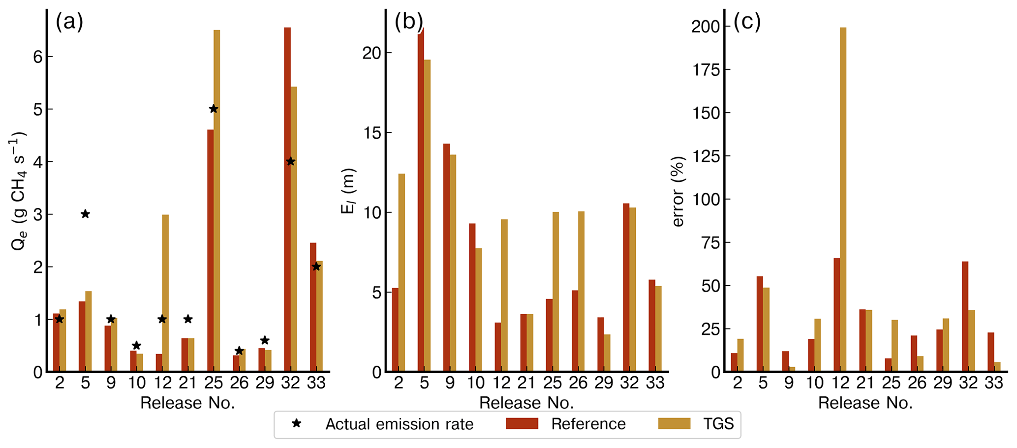
Figure A14Comparison of the emission rate estimates (Qe), location error (El), and relative error on the rate estimates for the inversions assimilating the reference data and the reconstruction of the CH4 from the TGS low-cost sensor based on the polynomial model of second degree.
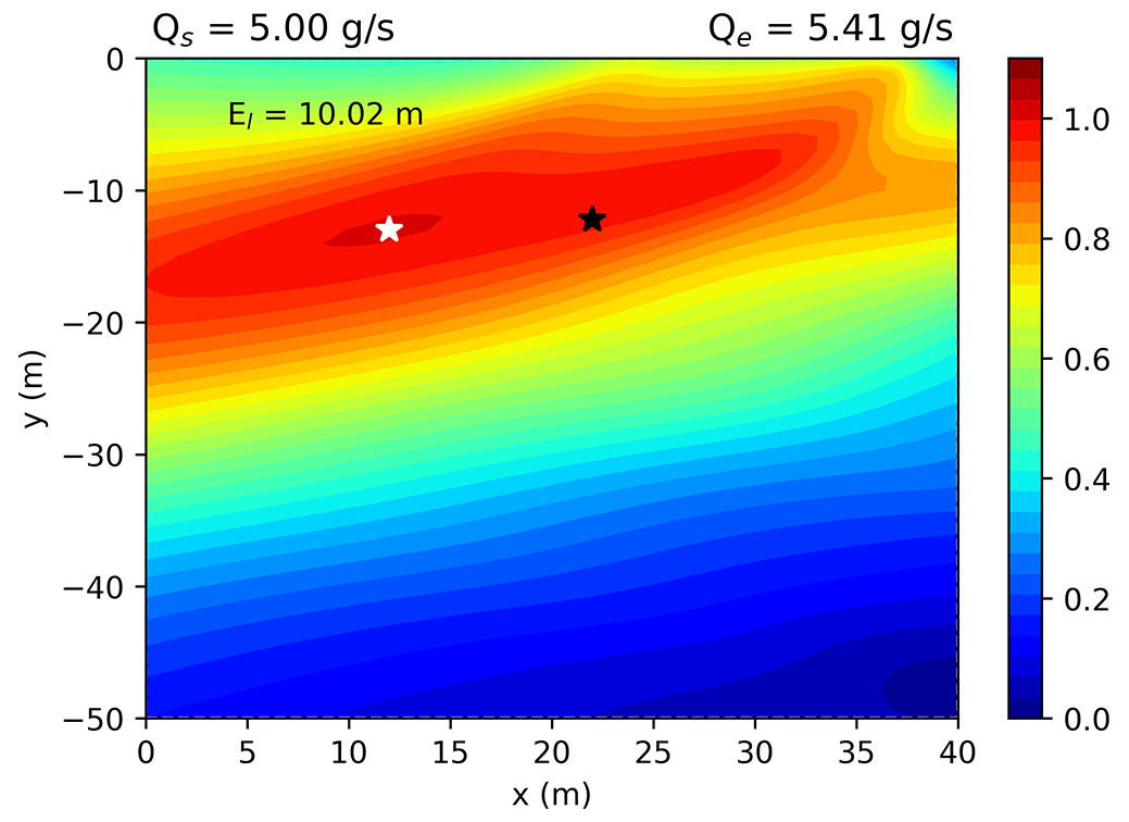
Figure A15Contour plot of the cost function for release no. 25 computed using assimilated gradients from TGS reconstructed data. The black and white stars shows the location of the actual and estimated location, respectively.
Table A1Distribution of the releases by chamber. For each chamber, the releases for which the TGS sensors produced valid measurements are denoted with “∘” and the invalid ones are denoted with “×”.
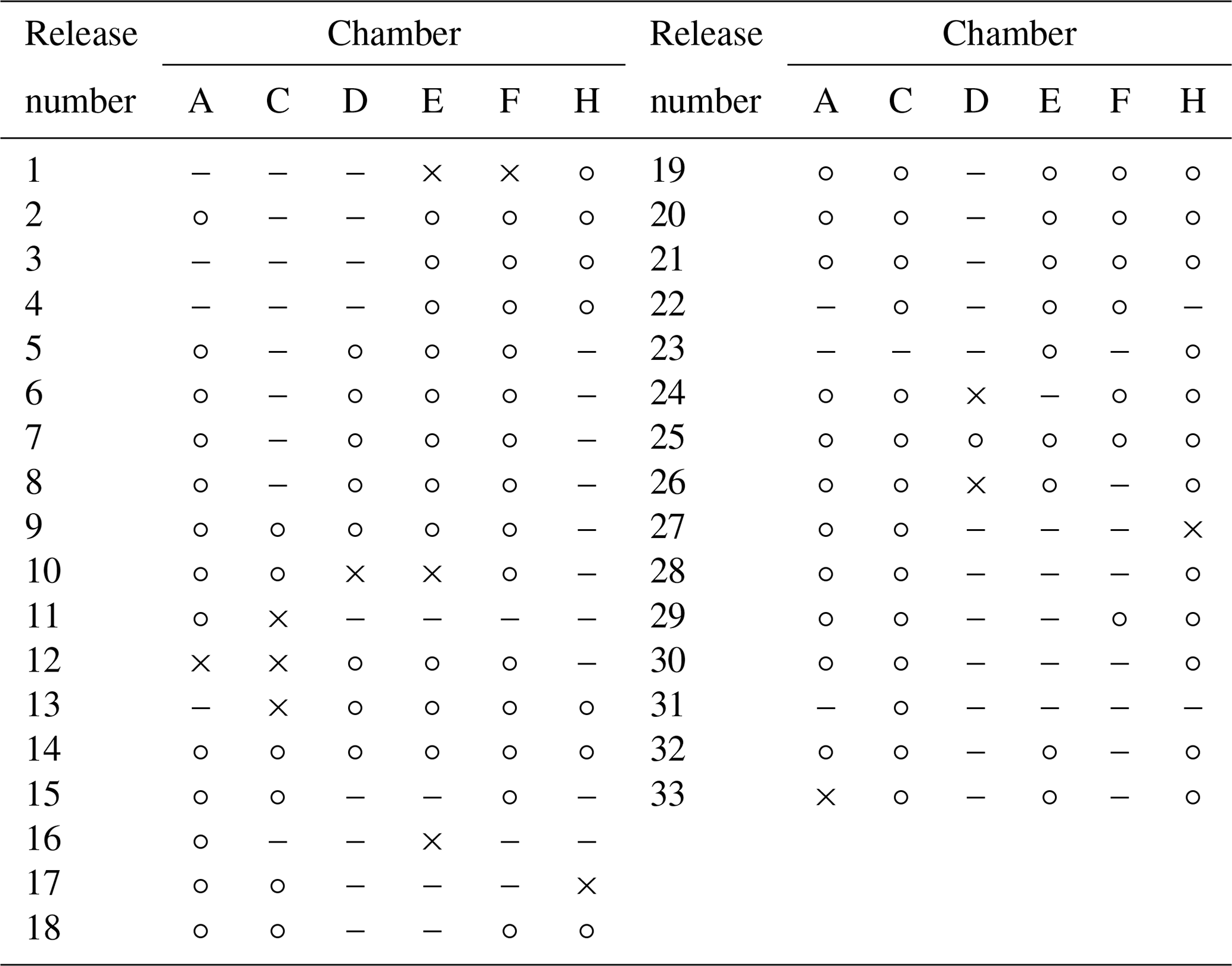
Table A2Comparison of the emission rate estimate (Qe), location error (El), and relative error of flux rate estimates for inversions assimilating reference gas analyser measurements and reconstructed TGS mole fractions using the second-degree polynomial model.
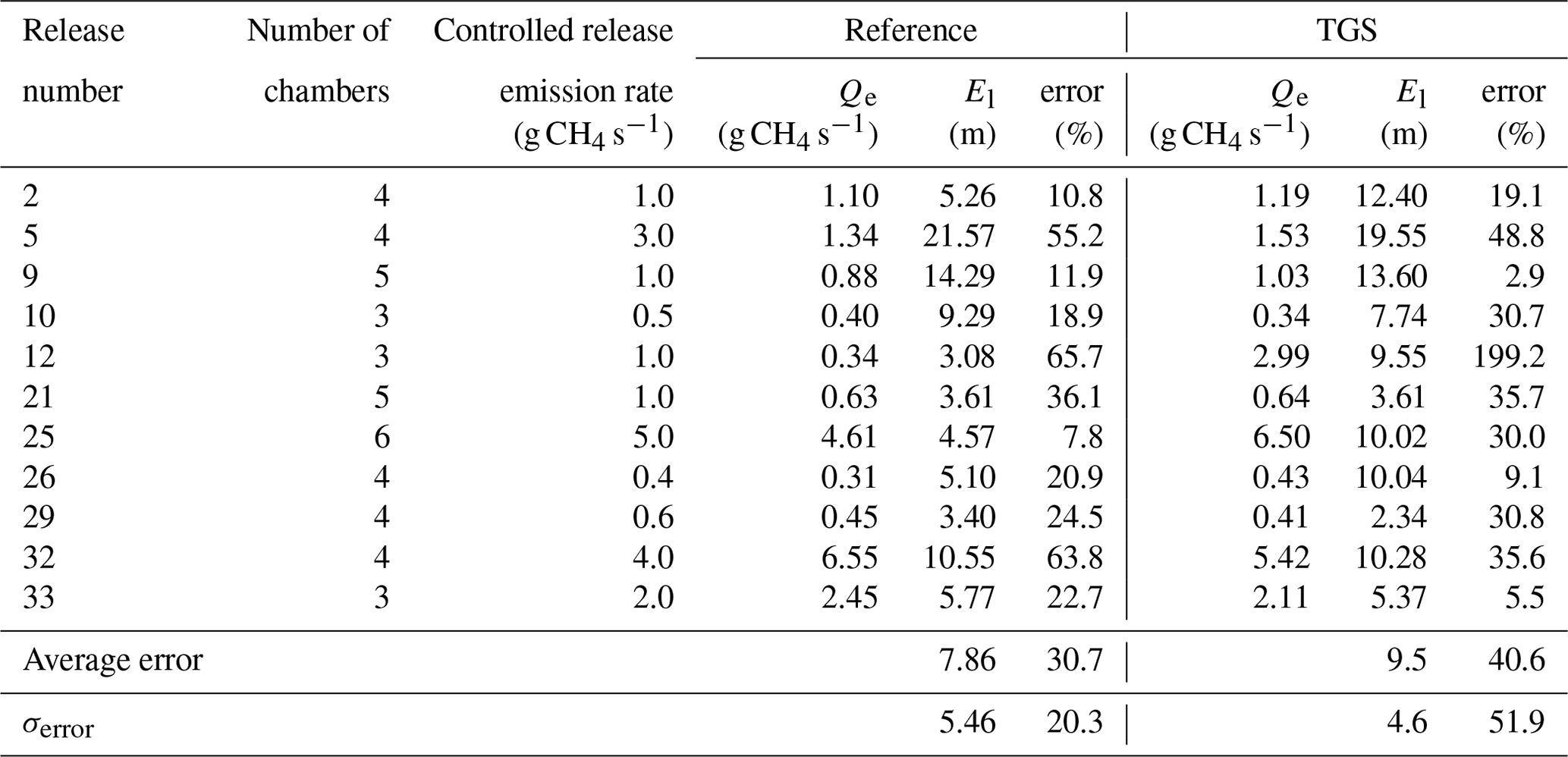
Table A3Summary of the tripods that were connected to each chamber.
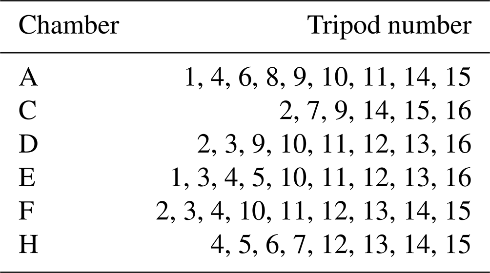
Table A4Comparison between TGS sensors included on the low-cost logging systems during the TADI 2019 campaign.
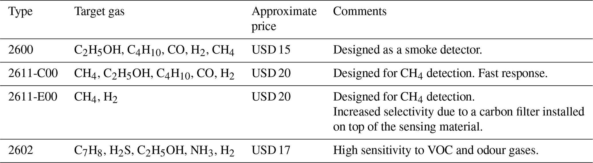
Table A5Summary of the species measured by each reference instrument.
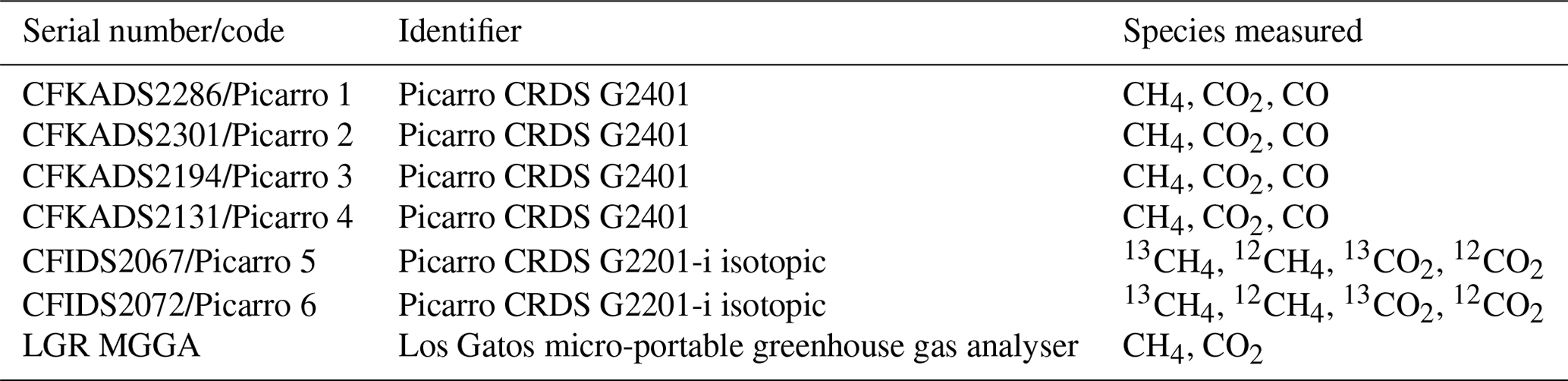
Table A6Summary of the specifications of the chambers, the tripods to which each chamber was connected, the captured releases, and the reference instrument collocated with each chamber.
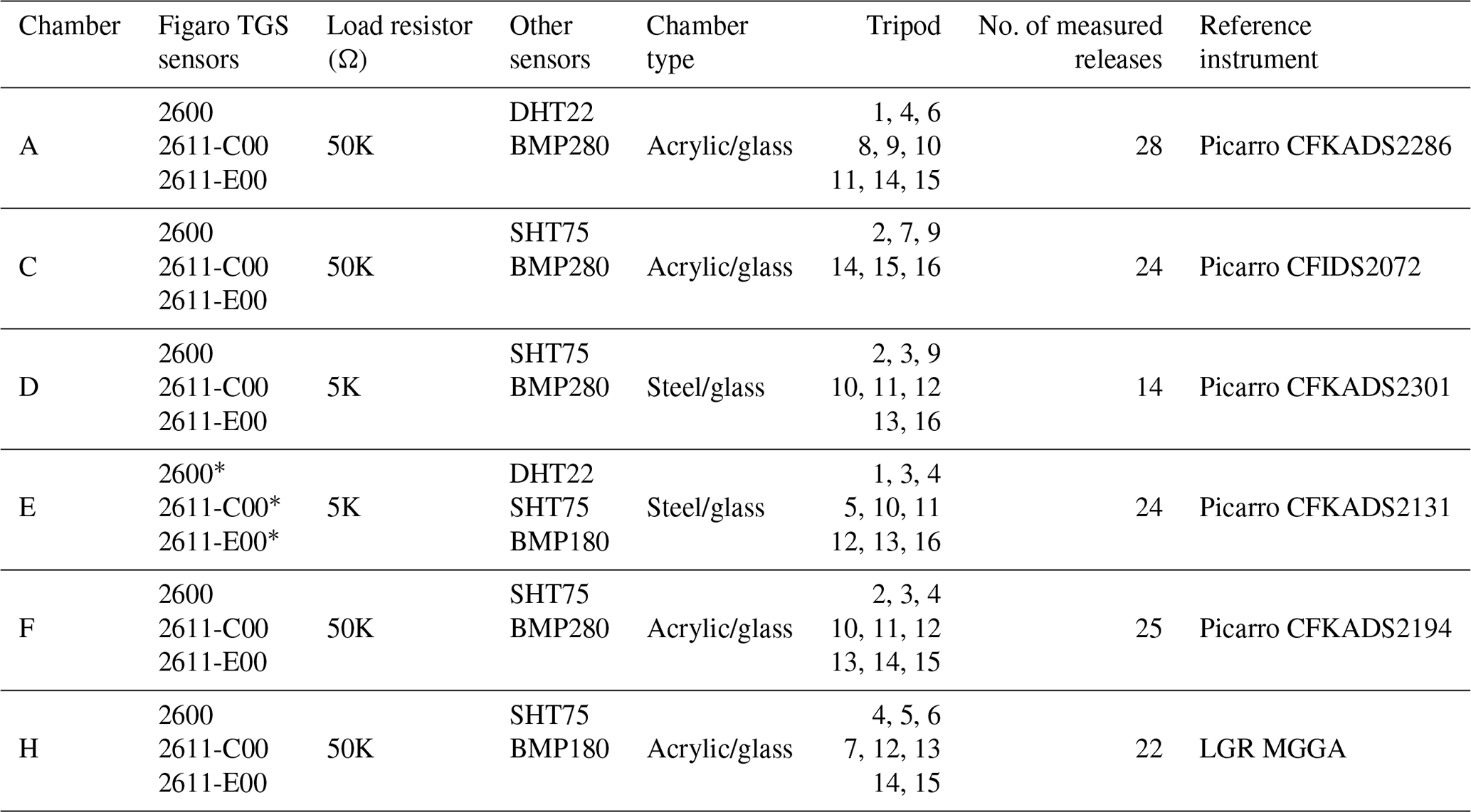
∗ Two versions of each type.
Table A7Computation time in seconds of the RSS matrix and the entire inversion including the preprocessing of the data for each release in the test set.
The codes were developed in the frame of the Chaire Industrielle TRACE ANR-17-CHIN-0004-01. They are accessible upon request to the corresponding author.
The data set was collected in the frame of the Chaire Industrielle TRACE ANR-17-CHIN-0004-01. It is publicly accessible at this link: https://doi.org/10.5281/zenodo.8399829 (Rivera Martinez et al., 2023b).
OL and FC designed the Figaro® logger system. OL, CC, and FC conducted the field measurement campaign. RRM and DS developed the CH4 reconstruction models. RRM, OL, and CM developed the baseline correction methodology of TGS sensors. PK and RRM developed the inversion framework to estimate the release locations and emission rates. RRM, GB, and PC prepared the manuscript with collaboration of the other co-authors.
The contact author has declared that none of the authors has any competing interests.
Publisher's note: Copernicus Publications remains neutral with regard to jurisdictional claims made in the text, published maps, institutional affiliations, or any other geographical representation in this paper. While Copernicus Publications makes every effort to include appropriate place names, the final responsibility lies with the authors.
This work was supported by the Chaire Industrielle Trace ANR-17-CHIN-0004-01 co-funded by the ANR French national research agency, TotalEnergies Raffinage Chimie, SUEZ – Smart & Environmental Solutions, and Thales Alenia Space.
This research has been supported by the Chaire Industrielle Trace, co-funded by the ANR, French national research agency, TotalEnergies Raffinage Chimie, SUEZ – Smart & Environmental Solutions, and Thales Alenia Space (grant no. ANR-17-CHIN-0004-01).
This paper was edited by Huilin Chen and reviewed by Pengfei Han and two anonymous referees.
Alvarez, R. A., Zavala-Araiza, D., Lyon, D. R., Allen, D. T., Barkley, Z. R., Brandt, A. R., Davis, K. J., Herndon, S. C., Jacob, D. J., Karion, A., Kort, E. A., Lamb, B. K., Lauvaux, T., Maasakkers, J. D., Marchese, A. J., Omara, M., Pacala, S. W., Peischl, J., Robinson, A. L., Shepson, P. B., Sweeney, C., Townsend-Small, A., Wofsy, S. C., and Hamburg, S. P.: Assessment of methane emissions from the U.S. oil and gas supply chain, Science, 361, eaar7204, https://doi.org/10.1126/science.aar7204, 2018. a, b
Bastviken, D., Nygren, J., Schenk, J., Parellada Massana, R., and Duc, N. T.: Technical note: Facilitating the use of low-cost methane (CH4) sensors in flux chambers – calibration, data processing, and an open-source make-it-yourself logger, Biogeosciences, 17, 3659–3667, https://doi.org/10.5194/bg-17-3659-2020, 2020. a, b
Bell, C., Ilonze, C., Duggan, A., and Zimmerle, D.: Performance of Continuous Emission Monitoring Solutions under a Single-Blind Controlled Testing Protocol, Environ. Sci. Technol., 57, 5794–5805, https://doi.org/10.1021/acs.est.2c09235, 2023. a, b
Bishop, C. M.: Neural Networks for Pattern Recognition, Oxford University Press, Inc., ISBN 0198538642, 1995. a
Casey, J. G., Collier-Oxandale, A., and Hannigan, M.: Performance of artificial neural networks and linear models to quantify 4 trace gas species in an oil and gas production region with low-cost sensors, Sensor. Actuat. B-Chem., 283, 504–514, https://doi.org/10.1016/j.snb.2018.12.049, 2019. a, b
Collier-Oxandale, A., Casey, J. G., Piedrahita, R., Ortega, J., Halliday, H., Johnston, J., and Hannigan, M. P.: Assessing a low-cost methane sensor quantification system for use in complex rural and urban environments, Atmos. Meas. Tech., 11, 3569–3594, https://doi.org/10.5194/amt-11-3569-2018, 2018. a, b
Collier-Oxandale, A. M., Thorson, J., Halliday, H., Milford, J., and Hannigan, M.: Understanding the ability of low-cost MOx sensors to quantify ambient VOCs, Atmos. Meas. Tech., 12, 1441–1460, https://doi.org/10.5194/amt-12-1441-2019, 2019. a
Eugster, W. and Kling, G. W.: Performance of a low-cost methane sensor for ambient concentration measurements in preliminary studies, Atmos. Meas. Tech., 5, 1925–1934, https://doi.org/10.5194/amt-5-1925-2012, 2012. a, b
Eugster, W., Laundre, J., Eugster, J., and Kling, G. W.: Long-term reliability of the Figaro TGS 2600 solid-state methane sensor under low-Arctic conditions at Toolik Lake, Alaska, Atmos. Meas. Tech., 13, 2681–2695, https://doi.org/10.5194/amt-13-2681-2020, 2020. a, b, c
Figaro®: TGS2600, Air Quality Sensor, Figaro (2005), https://www.figaro.co.jp/en/product/entry/tgs2600.html (last access: 10 February 2020), 2005. a
Figaro®: TGS2611-C00, Methane Sensor, Figaro (2013), https://www.figaro.co.jp/en/product/entry/tgs2611-c00.html (last access: 10 February 2020), 2013. a
Géron, A.: Hands-on machine learning with Scikit-Learn, Keras, and TensorFlow: Concepts, tools, and techniques to build intelligent systems, O'Reilly Media, ISBN 978-1-492-03264-9, 2019. a, b
Goodfellow, I., Bengio, Y., and Courville, A.: Deep Learning, MIT Press, http://www.deeplearningbook.org (last access: 30 March 2022), 2016. a
Haykin, S.: Neural Networks: A Comprehensive Foundation, Prentice Hall PTR, 2nd edn., ISBN 0132733501, 1998. a
Hornik, K., Stinchcombe, M., and White, H.: Multilayer feedforward networks are universal approximators, Neural Networks, 2, 359–366, https://doi.org/10.1016/0893-6080(89)90020-8, 1989. a
Kingma, D. P. and Ba, J.: Adam: A method for stochastic optimization, arXiv [preprint], https://doi.org/10.48550/arXiv.1412.6980, 22 December 2014. a
Kumar, P., Morawska, L., Martani, C., Biskos, G., Neophytou, M., Sabatino, S. D., Bell, M., Norford, L., and Britter, R.: The rise of low-cost sensing for managing air pollution in cities, Environ. Int., 75, 199–205, https://doi.org/10.1016/j.envint.2014.11.019, 2015. a
Kumar, P., Broquet, G., Yver-Kwok, C., Laurent, O., Gichuki, S., Caldow, C., Cropley, F., Lauvaux, T., Ramonet, M., Berthe, G., Martin, F., Duclaux, O., Juery, C., Bouchet, C., and Ciais, P.: Mobile atmospheric measurements and local-scale inverse estimation of the location and rates of brief CH4 and CO2 releases from point sources, Atmos. Meas. Tech., 14, 5987–6003, https://doi.org/10.5194/amt-14-5987-2021, 2021. a
Kumar, P., Broquet, G., Caldow, C., Laurent, O., Gichuki, S., Cropley, F., Yver‐Kwok, C., Fontanier, B., Lauvaux, T., Ramonet, M., Shah, A., Berthe, G., Martin, F., Duclaux, O., Juery, C., Bouchet, C., Pitt, J., and Ciais, P.: Near‐field atmospheric inversions for the localization and quantification of controlled methane releases using stationary and mobile measurements, Q. J. Roy. Meteor. Soc., 148, 1886–1912, https://doi.org/10.1002/qj.4283, 2022. a, b, c, d, e, f, g, h, i, j, k, l, m, n, o, p
Mead, M., Popoola, O., Stewart, G., Landshoff, P., Calleja, M., Hayes, M., Baldovi, J., McLeod, M., Hodgson, T., Dicks, J., Lewis, A., Cohen, J., Baron, R., Saffell, J., and Jones, R.: The use of electrochemical sensors for monitoring urban air quality in low-cost, high-density networks, Atmos. Environ., 70, 186–203, https://doi.org/10.1016/j.atmosenv.2012.11.060, 2013. a
Örnek, Ö. and Karlik, B.: An Overview of Metal Oxide Semiconducting Sensors in Electronic Nose Applications, IBU Repository, https://omeka.ibu.edu.ba/items/show/2364 (last access: 16 July 2024), 2012. a
Popoola, O. A., Carruthers, D., Lad, C., Bright, V. B., Mead, M. I., Stettler, M. E., Saffell, J. R., and Jones, R. L.: Use of networks of low cost air quality sensors to quantify air quality in urban settings, Atmos. Environ., 194, 58–70, https://doi.org/10.1016/j.atmosenv.2018.09.030, 2018. a
Riddick, S. N., Mauzerall, D. L., Celia, M., Allen, G., Pitt, J., Kang, M., and Riddick, J. C.: The calibration and deployment of a low-cost methane sensor, Atmos. Environ., 230, 117440, https://doi.org/10.1016/j.atmosenv.2020.117440, 2020. a, b, c, d
Riddick, S. N., Ancona, R., Cheptonui, F., Bell, C. S., Duggan, A., Bennett, K. E., and Zimmerle, D. J.: A cautionary report of calculating methane emissions using low-cost fence-line sensors, Elem. Sci. Anth., 10, 00021, https://doi.org/10.1525/elementa.2022.00021, 2022. a, b
Rivera Martinez, R., Santaren, D., Laurent, O., Cropley, F., Mallet, C., Ramonet, M., Caldow, C., Rivier, L., Broquet, G., Bouchet, C., Juery, C., and Ciais, P.: The Potential of Low-Cost Tin-Oxide Sensors Combined with Machine Learning for Estimating Atmospheric CH4 Variations around Background Concentration, Atmosphere, 12, 107, https://doi.org/10.3390/atmos12010107, 2021. a, b, c, d, e
Rivera Martinez, R. A., Santaren, D., Laurent, O., Broquet, G., Cropley, F., Mallet, C., Ramonet, M., Shah, A., Rivier, L., Bouchet, C., Juery, C., Duclaux, O., and Ciais, P.: Reconstruction of high-frequency methane atmospheric concentration peaks from measurements using metal oxide low-cost sensors, Atmos. Meas. Tech., 16, 2209–2235, https://doi.org/10.5194/amt-16-2209-2023, 2023a. a, b, c, d, e, f, g, h, i, j, k, l
Rivera Martinez, R. A., Kumar, P., Laurent, O., Broquet, G., Caldow, C., Cropley, F., Santaren, D., Shah, A., Mallet, C., Ramonet, M., Rivier, L., Juery, C., Duclaux, O., Bouchet, C., Allegrini, E., Utard, H., and Ciais, P.: Dataset for “Using Metal Oxide Gas Sensors for the Estimate of Methane Controlled Releases: Reconstruction of the Methane Mole Fraction Time-Series and Quantification of the Release Rates and Locations” (1.0.0), Zenodo [data set], https://doi.org/10.5281/zenodo.8399829, 2023b. a
Saunois, M., Stavert, A. R., Poulter, B., Bousquet, P., Canadell, J. G., Jackson, R. B., Raymond, P. A., Dlugokencky, E. J., Houweling, S., Patra, P. K., Ciais, P., Arora, V. K., Bastviken, D., Bergamaschi, P., Blake, D. R., Brailsford, G., Bruhwiler, L., Carlson, K. M., Carrol, M., Castaldi, S., Chandra, N., Crevoisier, C., Crill, P. M., Covey, K., Curry, C. L., Etiope, G., Frankenberg, C., Gedney, N., Hegglin, M. I., Höglund-Isaksson, L., Hugelius, G., Ishizawa, M., Ito, A., Janssens-Maenhout, G., Jensen, K. M., Joos, F., Kleinen, T., Krummel, P. B., Langenfelds, R. L., Laruelle, G. G., Liu, L., Machida, T., Maksyutov, S., McDonald, K. C., McNorton, J., Miller, P. A., Melton, J. R., Morino, I., Müller, J., Murguia-Flores, F., Naik, V., Niwa, Y., Noce, S., O'Doherty, S., Parker, R. J., Peng, C., Peng, S., Peters, G. P., Prigent, C., Prinn, R., Ramonet, M., Regnier, P., Riley, W. J., Rosentreter, J. A., Segers, A., Simpson, I. J., Shi, H., Smith, S. J., Steele, L. P., Thornton, B. F., Tian, H., Tohjima, Y., Tubiello, F. N., Tsuruta, A., Viovy, N., Voulgarakis, A., Weber, T. S., van Weele, M., van der Werf, G. R., Weiss, R. F., Worthy, D., Wunch, D., Yin, Y., Yoshida, Y., Zhang, W., Zhang, Z., Zhao, Y., Zheng, B., Zhu, Q., Zhu, Q., and Zhuang, Q.: The Global Methane Budget 2000–2017, Earth Syst. Sci. Data, 12, 1561–1623, https://doi.org/10.5194/essd-12-1561-2020, 2020. a
Shah, A., Laurent, O., Lienhardt, L., Broquet, G., Rivera Martinez, R., Allegrini, E., and Ciais, P.: Characterising the methane gas and environmental response of the Figaro Taguchi Gas Sensor (TGS) 2611-E00, Atmos. Meas. Tech., 16, 3391–3419, https://doi.org/10.5194/amt-16-3391-2023, 2023. a, b, c
Shah, A., Laurent, O., Broquet, G., Philippon, C., Kumar, P., Allegrini, E., and Ciais, P.: Determining methane mole fraction at a landfill site using the figaro taguchi gas sensor 2611-C00 and wind direction measurements, Environmental Science: Atmospheres, 4, 362–386, https://doi.org/10.1039/D3EA00138E, 2024. a, b
Singh, S. K., Sharan, M., and Issartel, J.-P.: Inverse modelling for identification of multiple-point releases from atmospheric concentration measurements, Bound.-Lay. Meteorol., 146, 277–295, https://doi.org/10.1007/s10546-012-9765-y, 2013. a
Travis, B., Dubey, M., and Sauer, J.: Neural networks to locate and quantify fugitive natural gas leaks for a MIR detection system, Atmos. Environ. X, 8, 100092, https://doi.org/10.1016/j.aeaoa.2020.100092, 2020. a
van den Bossche, M., Rose, N. T., and De Wekker, S. F. J.: Potential of a low-cost gas sensor for atmospheric methane monitoring, Sensor. Actuat. B-Chem., 238, 501–509, https://doi.org/10.1016/j.snb.2016.07.092, 2017. a
Yver Kwok, C., Laurent, O., Guemri, A., Philippon, C., Wastine, B., Rella, C. W., Vuillemin, C., Truong, F., Delmotte, M., Kazan, V., Darding, M., Lebègue, B., Kaiser, C., Xueref-Rémy, I., and Ramonet, M.: Comprehensive laboratory and field testing of cavity ring-down spectroscopy analyzers measuring H2O, CO2, CH4 and CO, Atmos. Meas. Tech., 8, 3867–3892, https://doi.org/10.5194/amt-8-3867-2015, 2015. a
- Abstract
- Introduction
- Methods
- Results
- Discussion
- Conclusions
- Appendix A: Models employed in the reconstruction of CH4 concentrations from TGS voltage measurements
- Code availability
- Data availability
- Author contributions
- Competing interests
- Disclaimer
- Acknowledgements
- Financial support
- Review statement
- References