A new non-linearity correction method for the spectrum from the Geostationary Inferometric Infrared Sounder on board Fengyun-4 satellites and its preliminary assessments

Non-linearity (NL) correction is a critical procedure to guarantee that the calibration accuracy of a spaceborne sensor approaches a reasonable level (i.e., better than 0.5 K). Unfortunately, such an NL correction is still not used in spectrum calibration from the Geostationary Interferometric InfraRed Sounder (GIIRS) onboard the Fengyun-4A (FY-4A) satellite. Different from the classical NL correction method where the NL coefficient is estimated from out-band spectral artifacts in an empirical low-frequency region, originally with prelaunch results and updated under in-orbit conditions, a new NL correction method for a spaceborne Fourier transform spectrometer (including GIIRS) is proposed. In particular, the NL parameter μ, independent of different working conditions (namely the thermal fields from environmental components), can be determined from laboratory results before launch and directly utilized during in-orbit calibration. Moreover, to overcome the inaccurate linear coefficient from the two-point calibration that influences the NL correction, an iteration algorithm is established to make both the linear and the NL coefficients converge to their stable values, with relative errors less than 0.5 % and 1 %, respectively, which is universally suitable for NL correction of both infrared and microwave sensors. Using the onboard internal blackbody (BB), which is identical to the in-orbit calibration, the final calibration accuracy for all the detectors and all the channels with the proposed NL correction method is validated to be around 0.2–0.3 K at an ordinary reference temperature of 305 K. Significantly, the relative error in the classical method NL parameter immediately transmitting to that of the linear one in theory, which inevitably introduces some additional errors around 0.1–0.2 K for the interfering radiance no longer exists. Moreover, the adopted internal BB with higher emissivity produces better NL correction performance in practice. The proposed NL correction method is scheduled for GIIRS implementation on board the FY-4A satellite and its successor after modifying their possible spectral response function variations.

1 Introduction

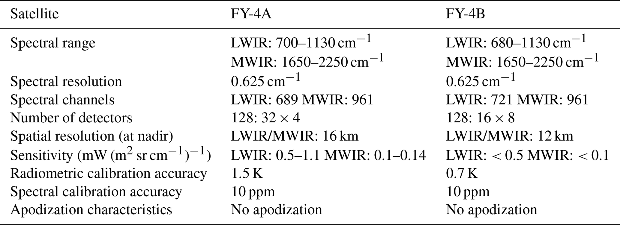
The Geostationary Interferometric Infrared Sounder (GIIRS), the first geostationary Fourier transform spectrometer (FTS), is on board the Fengyun-4A (FY-4A) satellite to provide high temporal resolution (on the order of 10¹–10² min) information on the atmospheric state for numerical weather prediction (NWP) and nowcasting, which is beneficial for monitoring and forecasting applications at regional scales (Guo et al., 2021b). Currently, there are two GIIRS-type sensors on board both FY-4A and Fengyun-4B (FY-4B), which were launched on 11 December 2016 and 3 June 2021, respectively. In general, the two sensors (namely FY-4A/GIIRS and FY-4B/GIIRS) are similar in their main spectral characteristics, i.e., the spectral resolution is 0.625 cm⁻¹, spectral calibration accuracy is 10 ppm, and spectral range and channels in the midwave infrared (MWIR) band are 1650–2250 cm⁻¹ and 961, respectively, except that the spectral range of longwave infrared (LWIR) of FY-4B/GIIRS was extended from the 700–1130 cm⁻¹ of FY-4A/GIIRS to 680–1130 cm⁻¹, and the corresponding spectral channels of FY-4B/GIIRS in the LWIR band have been increased by 32. Meanwhile, the total detector number of GIIRS for both the FY-4A and FY-4B satellites is the same – 128 – but it is the configurations of the detector arrays that differ from each other (i.e., 32×4 is for FY-4A/GIIRS and 16×8 for FY-4B/GIIRS). In particular, compared to FY-4A/GIIRS, both the radiometric and the geometrical characteristics (i.e., sensitivity, radiometric calibration accuracy, and spatial resolution) of FY-4B/GIIRS perform significantly better, as indicated in Table 1. Such improvements in FY-4B/GIIRS are expected to provide measurements from space with higher quality versus its predecessor. Domestic and international users have partially validated that the spectral and radiometric accuracies of the measured spectra from FY-4A/GIIRS V3 algorithm for L1 data show good performance for both the LWIR and MWIR bands (Guo et al., 2021b). However, the non-linearity (NL) correction has still not been implemented in the latest V3 algorithm. Therefore, in order to increase the radiometric accuracy further, a new NL correction method, which is aimed at carrying out the NL processing of GIIRS, is proposed in this article.

Table 1 Main specifications of LWIR and MWIR bands for GIIRS on board the FY-4A/B satellites.

The NL correction method ordinarily used for most FTSs is an approach first developed by the Space Science and Engineering Center at the University of Wisconsin–Madison (UW-SSEC; Han, 2018; Knuteson et al., 2004a; Qi et al., 2020). Measurements from an onboard FTS are affected by NL in different ways in different bands. In particular, for the LWIR and MWIR, the detectors have larger NL contributions to be corrected versus those of SWIR, which are negligibly small without correction (Qi et al., 2020; Zavyalov et al., 2011). Therefore, the NL correction for LWIR and MWIR bands of detectors is usually considered in most current research. In an FTS, the NL manifests itself as distortions of the resultant spectrum in the in-band spectral region. It also creates out-band spectral artifacts in the low-frequency region and at the harmonics of the in-band spectrum (Wu et al., 2020; Chase, 1984). Therefore, analysis of the spectral range between zero and the lowest-detectable wavenumber for the presence of spurious spectral response is an important diagnostic of the polynomial NL response in FTS measurements (Chase, 1984), although such a spurious spectral response does not have a strictly one-to-one correspondence with NL caused by the detector in theory. By looking for nonzero intensity in low-frequency regions where the detector response is known to be zero, the final NL coefficient can be obtained, i.e., for the Atmospheric Emitted Radiance Interferometer (AERI; Knuteson et al., 2004b). The approach has been applied to many interferometers, such as AERI (Knuteson et al., 2004a, b), the Cross-Track Infrared Sounder (CrIS; Han, 2018; Zavyalov et al., 2011; Taylor et al., 2009; Han et al., 2013), the High Spectral Infrared Atmospheric Sounder (HIRAS; Qi et al., 2020; Wu et al., 2020), the Thermal And Near infrared Sensor for carbon Observation Fourier-Transform Spectrometer (TANSO-FTS; Kuze et al., 2012), the Scanning High-rsolution Interferometer Sounder (S-HIS), and the National Airborne Sounder Testbed – Interferometer (NAST-I; Revercomb et al., 1998). In addition, there are also two other methods to determine the NL coefficient values, which have been applied to CrIS data. One of the methods uses the external blackbody (BB) calibration target (ECT) during prelaunch ground thermal vacuum tests, with the NL coefficient values determined from the spectra when the instrument views the ECT at a set of temperatures. The other one relies on a reference field of view (FOV) that has the lowest NL among the other FOVs and derives the NL coefficient values for the other FOVs relative to the reference FOV, which can be applied to both prelaunch and in-orbit calibrations (Han, 2018; Zavyalov et al., 2011; Tobin et al., 2013).

In fact, for a traditional broadband infrared sensor such as the Moderate Resolution Imaging Spectroradiometer (MODIS) the Geostationary Operational Environmental Satellite (GOES) imager, or the Visible Infrared Imaging Radiometer Suite (VIIRS; Datla et al., 2016; Oudrari et al., 2014; Xiong et al., 2003), the NL response must be determined and corrected during calibration, particularly the quadratic contribution of NL. Therefore, the quadratic NL coefficient for most infrared sensors is calculated in the laboratory calibration before launch and adopted directly for utilization under in-orbit conditions. Theoretically, however, both the linearity and the NL terms are affected by background radiation changes from the environmental components (Guo et al., 2021a) and the thermal fields that consist of different working conditions for a sensor (i.e., GIIRS), so the NL coefficient is not constant with respect to the linearity response. Meanwhile, to overcome the NL effects on the calibration accuracies of some microwave sensors, an optimized method is proposed where the receiver gain g and the system NL parameter μ are introduced in the calibration procedure. It implies that these calibration coefficients can be expressed well by g and μ, which have been widely used in most microwave sensors such as the Microwave Radiation Imager (MWRI), the Special Sensor Microwave Imager/Sounder (SSMIS), and the Special Sensor Microwave/Imager (SSM/I; Yang et al., 2011; Yan and Weng, 2008). Such an NL correction method for microwave sensors can provide a reference for infrared ones, although the linear coefficient calculated directly from measurements is inaccurate without the removal of the NL contribution.

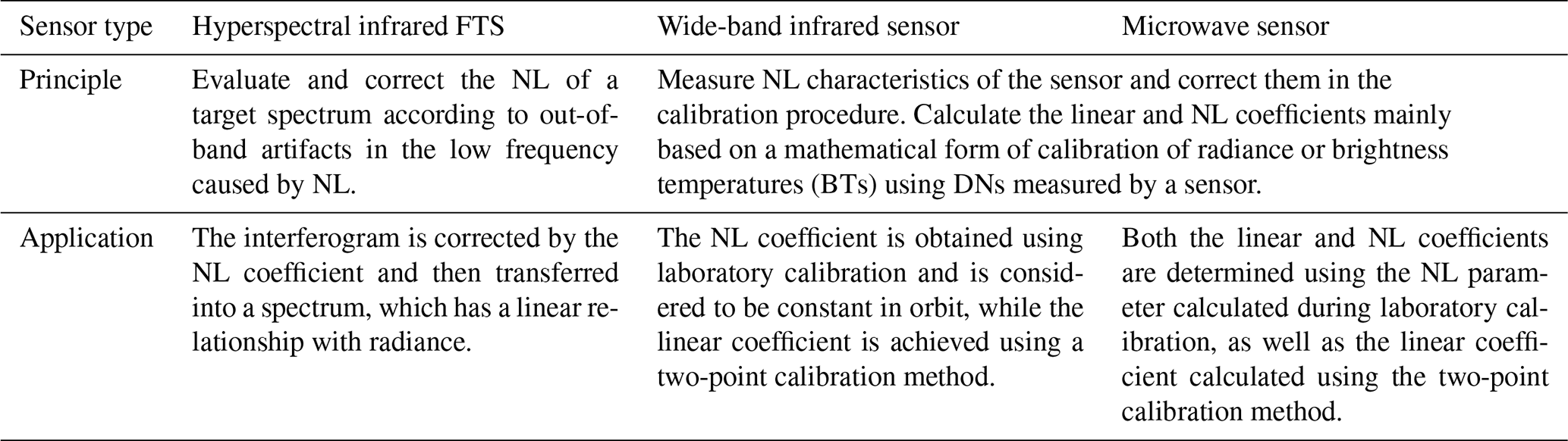
The NL principle of GIIRS is essentially the same as that of the traditional broadband sensors, except that the band (LWIR and MWIR) of GIIRS is much wider. Therefore, in this study, a new universal NL correction method is established for both FY-4A/GIIRS and FY-4B/GIIRS for most onboard infrared FTSs. There are two main steps in particular: firstly, based on the NL principle of infrared sensors (including GIIRS), the accurate linear and NL coefficients are calculated using laboratory results with an external high-accuracy BB after the spectral response function (SRF) of each GIIRS detector is estimated. Referring to the NL correction of microwave sensors, the NL parameter μ describing the relationship between the above linear and NL coefficients is subsequently determined. Secondly, an iterative algorithm is proposed to find the accurate NL coefficient, with both μ and the inaccurate linear one directly estimated using the two-point calibration method, which in theory provides a new and more accurate way for in-orbit NL correction for both infrared and microwave sensors. In Table 2, the main comparisons of NL correction methods for different types of sensors are provided in detail.

Table 2 Comparison of NL correction methods for different types of sensors.

2 Materials and methods

2.1 NL correction processing

As mentioned in Sect. 1, the NL correction of GIIRS is established by referring to the calibration method of the broadband infrared instruments, where the relationship between the output digital number (DN) and the received radiance (I) is usually expressed by the quadratic NL formula (Datla et al., 2016; Oudrari et al., 2014; Qi et al., 2012; Xiong et al., 2003), namely

$$\begin{array}{}\text{(1)}& I=a_{\mathrm{2}}\cdot {\mathrm{DN}}^{\mathrm{2}}+a_{\mathrm{1}}\cdot \mathrm{DN}+a_{\mathrm{0}},\end{array}$$

where a₀, a₁, and a₂ are the calibration coefficients. In general, coefficient a₀ for an ordinary measurement from a target (for example, the Earth's surface, a BB, or cold space) should be considered due to the influence of the actual dark current as well as the background radiance from the instrument itself. However, since the radiances of interest from the targets are their net ones, I in Eq. (1) is usually achieved by subtracting cold-space radiance from that of the target, which means that the alternating current (AC) component of target radiance is retained. Under this condition, it is acceptable that the a₀ coefficient in Eq. (1) is small enough to be negligible in this study.

Figure 1 Processing flow of the proposed NL correction.

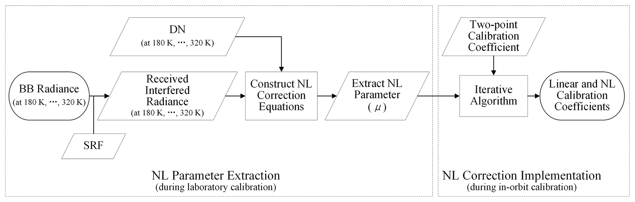
There are two steps of the proposed NL correction, i.e., NL parameter extraction (during laboratory calibration) and NL correction implementation (during in-orbit calibration), as shown in Fig. 1.

In the NL coefficient extraction step, after convolving BB radiance with the sensor's SRF, the theoretical interfering radiance (namely the interferogram) received by GIIRS can be obtained. Then, by aligning the subsample location, the measured interferogram will be converted into the optimized one with maximal DN, where its zero optical path difference (ZPD) misalignment can approach zero. Then, during laboratory calibration, NL coefficients (a₂) can be calculated by fitting the DN with the radiance at different temperatures (180, ..., 320 K) using the least-squares method. Finally, the NL parameter μ describing the relationship between the above linear and NL coefficients is determined for further in-orbit implementation.

In the second step, e.g., NL correction implementation during in-orbit calibration, firstly, the initial linear calibration coefficient is calculated using the two-point calibration method, the result of which is actually inaccurate without the removal of the NL contribution. Secondly, an iterative algorithm is adopted to generate the more-accurate linear and NL coefficients, with both the NL parameter μ and the initial two-point calibration result.

2.2 Principle and methods of NL correction for laboratory calibration

2.2.1 Observation principle of FTS

When implementing NL correction, firstly, we must determine the output DN with its corresponding received radiance using the sensor. As shown in Fig. 2, the typical Michelson interferometer system (i.e., GIIRS) includes a moving mirror, a stationary mirror, a beam splitter, a detector, and other elements, where the moving mirror and the stationary mirror are perpendicular to each other, and they are both at a 45° angle to the beam splitter. The incident radiance is divided into two parts using the beam splitter, with exactly the same vibration direction and frequency. One beam is incident on the stationary mirror and reflected, while the other beam is incident on the moving mirror and reflected. Then they pass through the beam splitter and reach the detector. The moving mirror moves back and forth linearly along the optical axis, which makes the optical path difference (OPD) of the two coherent beams change periodically. Finally, the detector receives an interferogram (known as interfering radiance) with continuous OPD over time. The DNs of the interferogram output from the detector are variable with different OPDs. In this study in particular, the resulting DN at the location of absolute ZPD is selected for calculation, where the radiation observed by the detector can be accurately calculated. Meanwhile, since the observation at absolute ZPD is usually unavailable due to some inevitable subsampling errors, the observed DN value at absolute ZPD can be adjusted from that at the location approaching ZPD.

Figure 2 A simple schematic diagram of the Michelson interferometer.

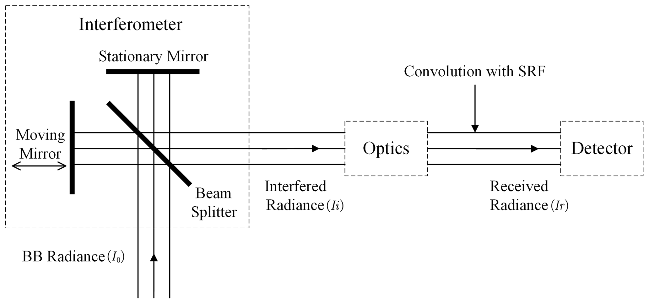
The radiance of the two interfering beams received by the detector is

$$\begin{array}{}\text{(2)}& \begin{array}{rl}{I}_i\left(T_n\right)=& I_{\mathrm{mov}}\left(T_n\right)+I_{\mathrm{sta}}\left(T_n\right)+\mathrm{2}\sqrt{I_{\mathrm{mov}}\left(T_n\right)\cdot I_{\mathrm{sta}}\left(T_n\right)}\\ & \cos \left(\mathrm{2}\mathit{\pi }\mathit{\upsilon }x\right),\end{array}\end{array}$$

where the υ is wavenumber, T_n is BB temperature, x is the OPD of the two beams, and I_mov and I_sta are the radiance of the two beams returned by the moving mirror and the stationary mirror passing through the beam splitter, which is the same and is half of the radiance (I₀) incident to the interferometer, that is $I_{\mathrm{mov}}=I_{\mathrm{sta}}=(\mathrm{1}/\mathrm{2})I_{\mathrm{0}}$. As at the ZPD location, the OPD x=0 and the radiance is maximal, which means

$$\begin{array}{}\text{(3)}& I_i\left(T_n\right)=I_{\mathrm{0}}\left(T_n\right)\left[\mathrm{1}+\cos \left(\mathrm{2}\mathit{\pi }\mathit{\upsilon }x\right)\right]=\mathrm{2}{I}_{\mathrm{0}}\left(T_n\right),\end{array}$$

where I₀ is the theoretical BB radiance from the laboratory calibration and according to the Planck's blackbody law,

$$\begin{array}{}\text{(4)}& I_{\mathrm{0}}\left(T_n,\mathit{\nu }\right)={\displaystyle \frac{c_{\mathrm{1}}{\mathit{\nu }}^{\mathrm{3}}}{{\mathrm{e}}^{c_{\mathrm{2}}\mathit{\nu }/T_n}-\mathrm{1}}}\cdot {\mathit{\epsilon }}_{\mathrm{b}}\left(\mathit{\nu }\right),\end{array}$$

where $c_{\mathrm{1}}=\mathrm{1.191}\times {\mathrm{10}}^{-\mathrm{5}}$ W cm², c₂=1.439 cm K, ε_b(ν) is the emissivity of the laboratory BB for different wavenumbers, and the units for I₀ are m W (m² sr cm⁻¹)⁻¹.

To calculate the radiance within the whole responsive band of the sensor, the theoretical BB radiance needs to have a convolution with SRF, i.e.,

$$\begin{array}{}\text{(5)}& I_{\mathrm{r}}\left(T_n\right)=\mathrm{2}\cdot {\displaystyle \frac{{\int }_{{\mathit{\nu }}_{\mathrm{1}}}^{{\mathit{\nu }}_{\mathrm{2}}}\mathrm{srf}\left(\mathit{\nu }\right)\cdot I_{\mathrm{0}}\left(T_n,\mathit{\nu }\right)\mathrm{d}\mathit{\nu }}{{\int }_{{\mathit{\nu }}_{\mathrm{1}}}^{{\mathit{\nu }}_{\mathrm{2}}}\mathrm{srf}\left(\mathit{\nu }\right)\mathrm{d}\mathit{\nu }}},\end{array}$$

where I_r is the received radiance, ν₁ and ν₂ are the beginning and ending wavenumber of the whole band, and srf(ν) is the SRF for each wavenumber, which will be given in Sect. 3.2.1. Furthermore, for the term I_r(T_n) in Eq. (5), which is the theoretical radiance observed by GIIRS at the absolute ZPD location, no correction in practice is required for the off-axis effect on this term.

2.2.2 Subsample location alignment

After the theoretical radiance received by the sensor is obtained, it is important to determine the theoretical ZPD location to find the maximal value of the interferogram with its phase misalignment approaching zero.

For the discretely sampled interferogram value (I(k)) with its ZPD at the k₀th sample location, the discrete integer (k₀) is highly likely to be misaligned versus its true ZPD value by a certain subsample-scale offset. In order to remove such a misalignment, I(k) can be first oversampled β times (i.e., β can be set to be 100 or more) into I_β(k). Then, when applying the same ZPD detection method to I_β(k) as used for I(k), the ZPD location of I_β(k), that is, k_β, can be easily determined. Hence, Δk₀ was given by Guo et al. (2021b) as

$$\begin{array}{}\text{(6)}& \mathrm{\Delta }{k}_{\mathrm{0}}=(k_{\mathrm{0}}\cdot \mathit{\beta }-k_{\mathit{\beta }})/\mathit{\beta }.\end{array}$$

Moreover, supposing that I(ξ) is the discrete Fourier transform (DFT) of I(k), it means

$$\begin{array}{}\text{(7)}& \left\{\begin{array}{l}I\left(\mathit{\xi }\right)=F\left[I\left(k\right)\right]={\sum }_{k=\mathrm{0}}^{N-\mathrm{1}}I\left(k\right)\cdot {\mathrm{e}}^{-j\cdot \left(\frac{\mathrm{2}\mathit{\pi }k}{N}\right)\cdot \mathit{\xi }},\\ \mathit{\xi }\in [\mathrm{0},N-\mathrm{1}]\\ I\left(k\right)=F^{-\mathrm{1}}\left[I\left(\mathit{\xi }\right)\right]=\frac{\mathrm{1}}{N}{\sum }_{\mathit{\xi }=\mathrm{0}}^{N-\mathrm{1}}I\left(\mathit{\xi }\right)\cdot e^{j\cdot \left(\frac{\mathrm{2}\mathit{\pi }\mathit{\xi }}{N}\right)\cdot k},\\ k\in [\mathrm{0},N-\mathrm{1}]\end{array}\right.,\end{array}$$

where F[⋅] and $F^{-\mathrm{1}}\left[\cdot \right]$ represent the DFT and inverse DFT (IDFT), respectively, and N is the sampling number. In particular, since the off-axis angle (θ) spans the vectors pointing from the location of a detector to the focal point of optics and the main optical axis, different ones will make effective optical path differences in detectors quite different from each other, even for the same interference pattern introduced by GIIRS. The off-axis effects ultimately result in the different spectral resolutions among individual detectors without corrections. Therefore, according to the principle of an FTS with double-side interferograms (i.e., GIIRS), for both a given cos(θ) related to an individual detector and a required spectral resolution of Δυ, the sampling number (N) is satisfied by

$$\begin{array}{}\text{(8)}& N=\mathrm{int}\left\{{\displaystyle \frac{\mathrm{10}\mathrm{000}}{\cos \left(\mathit{\theta }\right)\cdot \mathrm{\Delta }\mathit{\nu }\cdot {\mathit{\lambda }}_{\mathrm{laser}}}}+\mathrm{0.5}\right\},\end{array}$$

where θ is the off-axis angle, and cos(θ) values of each detector for both forward and backward travel of the moving mirror are accurately measured in prelaunch testing. The Δν=0.625 cm⁻¹ is the required spectral resolution and the λ_laser=0.85236 µm is the reference laser wavelength in microns.

According to the properties of DFT, Eq. (7) can also be written as

$$\begin{array}{}\text{(9)}& I(k_{\mathrm{0}}-\mathrm{\Delta }{k}_{\mathrm{0}})=F^{-\mathrm{1}}[\left(e^{-j\cdot \mathrm{\Delta }{k}_{\mathrm{0}}\cdot \frac{\mathrm{2}\mathit{\pi }\mathit{\xi }}{N}}\right)\cdot I\left(\mathit{\xi }\right)],\end{array}$$

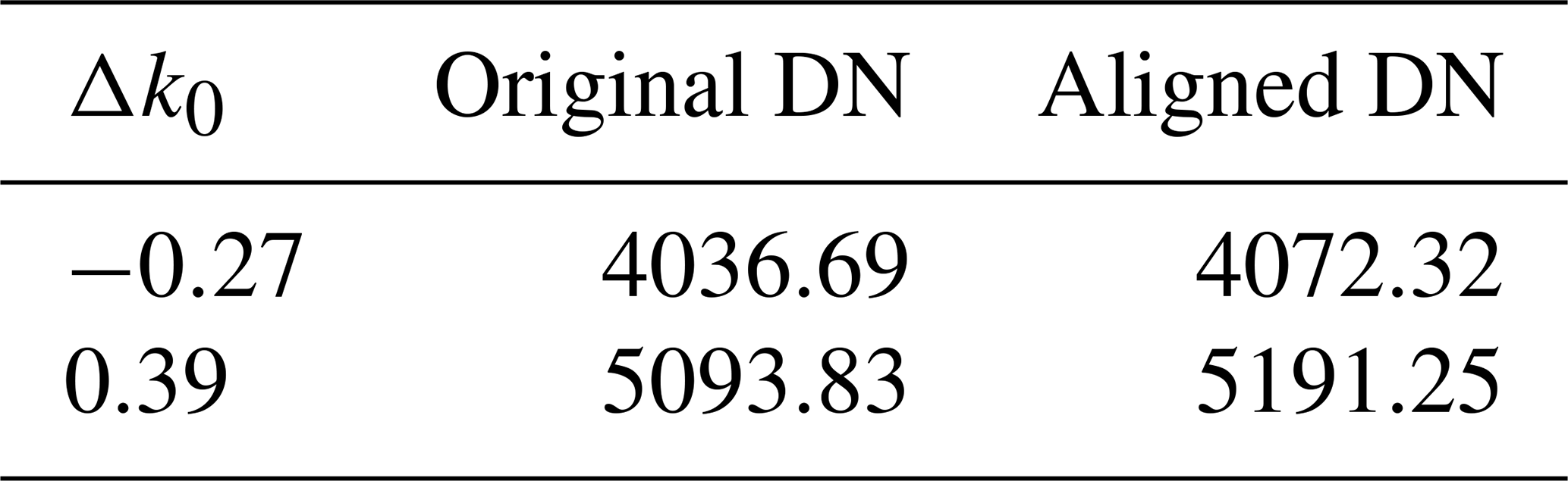
where I(ξ) is the DFT of I(k). Therefore, any measured interferogram (I(k)) can be converted in order to have a smaller ZPD misalignment, which is no more than 1/2β of the sample location in theory. The symmetry of the aligned interferogram will be significantly improved. Some examples of DNs before (original) and after (aligned) subsample location alignment are list in Table 3. Obviously, different misalignments will generate different aligned DNs compared to their original ones, where the relative errors are between approximately 1 % and 2 %, with misalignment of more than 0.4 samples.

Table 3 Examples of DNs before and after subsample location alignment.

2.2.3 Calculation method of NL coefficients

After the theoretical received radiance (I_r) and the maximal DN value (DN_m) at absolute ZPD are obtained, the NL coefficient is solved using measurements from several external BB sources with different temperatures, which means that

$$\begin{array}{}\text{(10)}& \left\{\begin{array}{l}{I}_{\mathrm{r}}\left(T_{\mathrm{1}}\right)=a_{\mathrm{2}}\cdot {\mathrm{DN}}_{\mathrm{m}}^{\mathrm{2}}\left(T_{\mathrm{1}}\right)+a_{\mathrm{1}}\cdot {\mathrm{DN}}_{\mathrm{m}}\left(T_{\mathrm{1}}\right)\\ \mathrm{\dots }\\ I_{\mathrm{r}}\left(T_n\right)=a_{\mathrm{2}}\cdot {\mathrm{DN}}_{\mathrm{m}}^{\mathrm{2}}\left(T_n\right)+a_{\mathrm{1}}\cdot {\mathrm{DN}}_{\mathrm{m}}\left(T_n\right)\end{array}\right.,\end{array}$$

where T₁, ..., T_n are different BB temperatures from 180 to 320 K. To remove the influence of the background on hot BB measurements(with temperatures higher than 180 K), I_r and DN_m are subtracted from a cold BB observation with a temperature around 80 K, resulting in both the net radiation and the DN with respect to the hot temperatures, where the radiation from the cold BB itself is negligible compared to the background of the sensor.

It should be emphasized that cos(θ) values for the two sweep directions (forward or reverse) differ from each other even for the same detector, which means that off-axis correction for different directions should be performed with the corresponding cos(θ) in order to standardize the spectral scales for different detectors and different directions. Theoretically, off-axis correction aims to determine how many samples of an interferogram should be applied for such a DFT procedure to obtain the uniform spectral scales of spectra from targets with different detectors as well as different sweep directions. Actually, the a₂ and a₁ coefficients in Eq. (10) are utilized to describe the radiometric response characteristics of an individual detector, which are independent of Michelson interferometric optics. After implementing the subsample location alignment for both forward and reverse sweeps as indicated in Sect. 2.2.2, all interferograms from the same detector in both directions are used to achieve the summed ones with lower noise levels. Therefore, in Eq. (10), considering that I_r(T_n) is the inferred radiance at the absolute ZPD location, it should not be corrected for the off-axis effect.

After the laboratory calibration coefficients a₁ and a₂ are obtained, the NL correction methods for microwave instruments are referenced, where the relationship between the linear and the NL coefficients are selected to generate an NL parameter (μ) describing the NL characteristic of the sensor. In particular, for a microwave instrument, there is a calibration gain g calculated by the two-point calibration method (Yan and Weng, 2008; Yang et al., 2011), which is equal to the linear coefficient a₁ in mathematics, i.e.,

$$\begin{array}{}\text{(11)}& a_{\mathrm{1}}=g={\displaystyle \frac{I_{\mathrm{h}}-I_{\mathrm{c}}}{{\mathrm{DN}}_{\mathrm{h}}-{\mathrm{DN}}_{\mathrm{c}}}},\end{array}$$

where I_h and I_c are the radiances of hot and cold BBs and DN_h and DN_c are the corresponding DNs.

Here, the NL calibration coefficient (a₂) can be expressed by the gain and the NL parameter (μ) for a microwave sensor, namely

$$\begin{array}{}\text{(12)}& a_{\mathrm{2}}=\mathit{\mu }\cdot g^{\mathrm{2}},\end{array}$$

where the NL parameter (μ) describes the NL characteristic of a sensor itself. It denotes the relationship between the linear and NL coefficients obtained from the contribution of the linear and NL parts to the whole radiometric response of a sensor, representing the shape feature of the NL curve unrelated to radiance from targets, which is in theory ordinarily independent of the different working conditions of a sensor.

In fact, the basic mathematic expression of NL characteristics of a microwave sensor is fully identical to that of an infrared one (i.e., GIIRS), where calculations of both the linear and the NL coefficients are mainly based on the mathematical form of radiometric calibrations of radiance or brightness temperature (BT), with DNs measured by a sensor. Thus, the μ-parameter method adopted for a microwave sensor can be referenced for application to an infrared one. Moreover, the NL coefficients in infrared sensors are actually inconstant, while the NL parameter μ representing the relationship between the linear (a₁) and NL (a₂) coefficients is generally more stable (the comparison results are shown in Table 4 in Sect. 3.2.2.), which is more suitable for description of the NL characteristics of an infrared sensor.

Therefore, the NL parameter (μ) introduced in this method can be defined as

$$\begin{array}{}\text{(13)}& \mathit{\mu }=a_{\mathrm{2}}/g^{\mathrm{2}}=a_{\mathrm{2}}/a_{\mathrm{1}}^{\mathrm{2}}.\end{array}$$

By calculating the mean value of the laboratory calibration coefficients, the final NL parameter μ can be obtained.

2.3 A new iterative algorithm for in-orbit NL correction

In general, the NL coefficients of most broadband infrared sensors from laboratory calibration before launch are directly applied in orbit. However, it is inaccurate to use the laboratory coefficients directly.

Figure 3 The iterative algorithm flow of in-orbit NL correction.

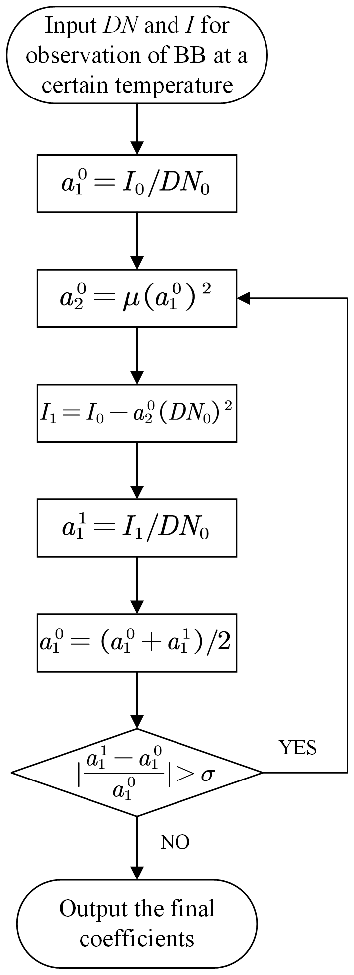
In fact, although the NL parameter μ is introduced to generate the variable NL coefficient a₂ together with the linear one from Eq. (13), the coefficient of a₁ is usually achieved by means of the two-point calibration method, where the NL influence cannot be removed completely. Therefore, an iterative algorithm is proposed in this study: by dynamically modifying the quadratic NL term (a₂), the linear coefficient is calculated continuously in order to approach a stable one, and final, accurate linear and NL coefficients can be obtained. The detailed diagram is shown in Fig. 3.

The initial linear calibration coefficient $a_{\mathrm{1}}^{\mathrm{0}}$ at a certain temperature is obtained.

Using $a_{\mathrm{1}}^{\mathrm{0}}$ and the NL parameter μ from laboratory results, the initial NL coefficient $a_{\mathrm{2}}^{\mathrm{0}}$ can be generated.

Subtracting the calculated NL contribution from the original radiance I₀, the corrected radiance I₁ can be obtained.

The corrected linear coefficient $a_{\mathrm{1}}^{\mathrm{1}}$ can be calculated using I₁ and the initial DN₀.

The mean value between $a_{\mathrm{1}}^{\mathrm{0}}$ and $a_{\mathrm{1}}^{\mathrm{1}}$ is used as an updated $a_{\mathrm{1}}^{\mathrm{0}}$.

If the relative deviation of the two linear coefficients ($a_{\mathrm{1}}^{\mathrm{0}}$ and $a_{\mathrm{1}}^{\mathrm{1}}$) is greater than the threshold σ (σ is dependent on the required accuracy; i.e., σ can be set as 0.001), a new or updated a₂ can be obtained using the updated $a_{\mathrm{1}}^{\mathrm{0}}$.

Otherwise, when the deviation is less than the threshold σ, the current linear coefficient a₁ is acceptable, while the target NL coefficient a₂ can be also calculated correspondingly.

2.4 NL coefficient extraction using the classical method

For the classical method of NL correction, the anomalous spectra affected by the NL response of an FTS (i.e., GIIRS) in the low-frequency part is used to correct the quadratic NL, similar to methods in the relevant literature (Han, 2018; Han et al., 2013; Knuteson et al., 2004a; Tobin et al., 2013). In particular, the out-of-band low-frequency spectrum of 50–450 cm⁻¹ is empirically selected for calculation.

An interferogram from a detector with certain NL characteristics may be related to the ideal interferogram DN_ia from a linear detector using the following model (Han, 2018) as

$$\begin{array}{}\text{(14)}& {\mathrm{DN}}_{\mathrm{ia}}+{\mathrm{DN}}_{\mathrm{id}}=\left({\mathrm{DN}}_{\mathrm{ma}}+{\mathrm{DN}}_{\mathrm{md}}\right)+b_{\mathrm{2}}{\left({\mathrm{DN}}_{\mathrm{ma}}+{\mathrm{DN}}_{\mathrm{md}}\right)}^{\mathrm{2}},\end{array}$$

where DN_ia and DN_ma are defined as the ideal and measured output AC voltage in volts, DN_id and DN_md are the direct current (DC) voltage, and b₂ is the NL coefficient from the classical method. Since the DC term has no contribution to the spectrum of interest, Eq. (14) can be rewritten as

$$\begin{array}{}\text{(15)}& {\mathrm{DN}}_{\mathrm{ia}}=\left(\mathrm{1}+\mathrm{2}{b}_{\mathrm{2}}{\mathrm{DN}}_{\mathrm{md}}\right){\mathrm{DN}}_{\mathrm{ma}}+b_{\mathrm{2}}{\mathrm{DN}}_{\mathrm{ma}}^{\mathrm{2}}.\end{array}$$

Implementing DFT on both sides of Eq. (15), the corresponding spectra can be obtained,

$$\begin{array}{}\text{(16)}& S_{\mathrm{ia}}=\left(\mathrm{1}+\mathrm{2}{b}_{\mathrm{2}}{\mathrm{DN}}_{\mathrm{md}}\right)S_{\mathrm{ma}}+b_{\mathrm{2}}{S}_{\mathrm{ma}}\otimes S_{\mathrm{ma}},\end{array}$$

where S_ia is the ideal spectrum, S_ma is the measured spectrum, and S_ma⊗S_ma is the self-convolution of S_ma. Assuming that the ideal spectrum of the out-of-band spectrum is 0, Eq. (16) can be rewritten as

$$\begin{array}{}\text{(17)}& \mathrm{0}=\left(\mathrm{1}+\mathrm{2}{b}_{\mathrm{2}}{\mathrm{DN}}_{\mathrm{md}}\right)S_{\mathrm{ma}}+b_{\mathrm{2}}{S}_{\mathrm{ma}}\otimes S_{\mathrm{ma}}.\end{array}$$

Therefore, the NL coefficient b₂ can be given as

$$\begin{array}{}\text{(18)}& b_{\mathrm{2}}={\displaystyle \frac{b_{\mathrm{2}}^{{}^{\prime }}}{\mathrm{1}-\mathrm{2}{b}_{\mathrm{2}}^{{}^{\prime }}{\mathrm{DN}}_{\mathrm{md}}}},\end{array}$$

where $b_{\mathrm{2}}^{{}^{\prime }}=-S_{\mathrm{ma}}/S_{\mathrm{ma}}\otimes S_{\mathrm{ma}}$.

3 Results

3.1 Introduction to experimental data and instruments

In order to evaluate the proposed NL correction method more accurately, the experimental data of FY-4B/GIIRS between 13 January and 11 February 2020 (namely the laboratory test/calibration results in a vacuum chamber before launch) were obtained to calculate the NL parameter μ for different detectors, which have been utilized to implement the radiometric calibration together with the corresponding measurements from the internal hot BB target in both in-orbit and in-lab conditions. It should be mentioned, as shown in Fig. 4, that measurements from both the external and the internal BB targets were switched with each other when the scanning mirror was rotated by 90 degrees under certain stable GIIRS situations.

Figure 4 Sketch of the GIIRS laboratory test in a vacuum chamber.

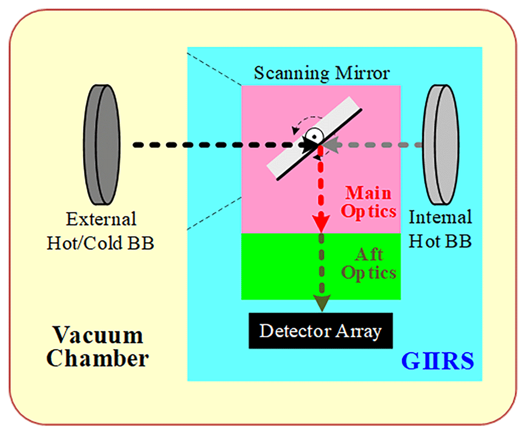
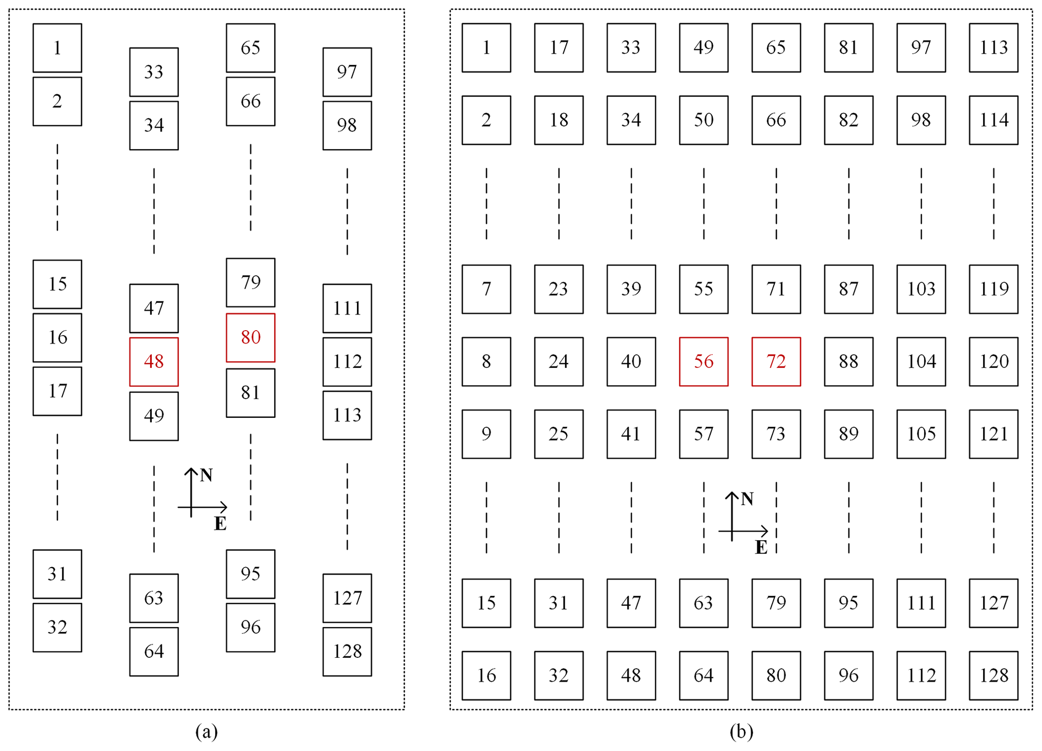
Figure 5 Layouts of the detector arrays for GIIRS on board different satellites: (a) FY-4A and (b) FY-4B.

Meanwhile, as listed in Table 1, although the total detector numbers of the LWIR or the MWIR bands of both FY-4A/GIIRS and FY-4B/GIIRS are the same (i.e., 128), the layouts of the detector arrays for the two sensors are quite different, as shown in Fig. 5. The main difference is that the detector number for one column in the north–south direction has been decreased from 32 for FY-4A to 16 for FY-4B, while the column number in the east–west direction has been increased correspondingly, from 4 for FY-4A to 8 for FY-4B. Such a change in theory reduces the spectral inconsistencies among different detectors due to the different off-axis angles caused by the detector array itself. In particular, the detectors (48 and 80, marked in red) near the central FOV in FY-4A are also transformed into others (56 and 72, marked in red) in FY-4B.

During the in-lab test, the calibration procedures for FY-4B/GIIRS were scheduled to be done under three scenarios for the main optics (including the scanning and the different reflective mirrors), namely normal, cold and hot conditions, to assess the possible variations in the radiometric response of GIIRS under different conditions. However, for each condition, the aft optics (including the interferometer) were maintained at optimal temperature conditions (i.e., around 200 K for the interferometer and 65–75 K for the optical assemblies related to detectors). In particular, the approximate temperature ranges of −15 to −10, 0 to 5, and 10 to 15 °C correspond to the cold, normal, and hot conditions, respectively.

3.2 NL coefficient and parameter extraction using the proposed method

3.2.1 Calculation of SRF

The SRF of a sensor (i.e., GIIRS) generally refers to the ratio of the received radiation relative to the incident radiation at each wavenumber. In this study, the SRF of the broad band of GIIRS can be obtained using laboratory calibration data. The SRF of each wavenumber can be given by

$$\begin{array}{}\text{(19)}& \mathrm{srf}\left(\mathit{\nu }\right)=S\left(\mathit{\nu }\right)/I_{\mathrm{0}}\left(\mathit{\nu }\right),\end{array}$$

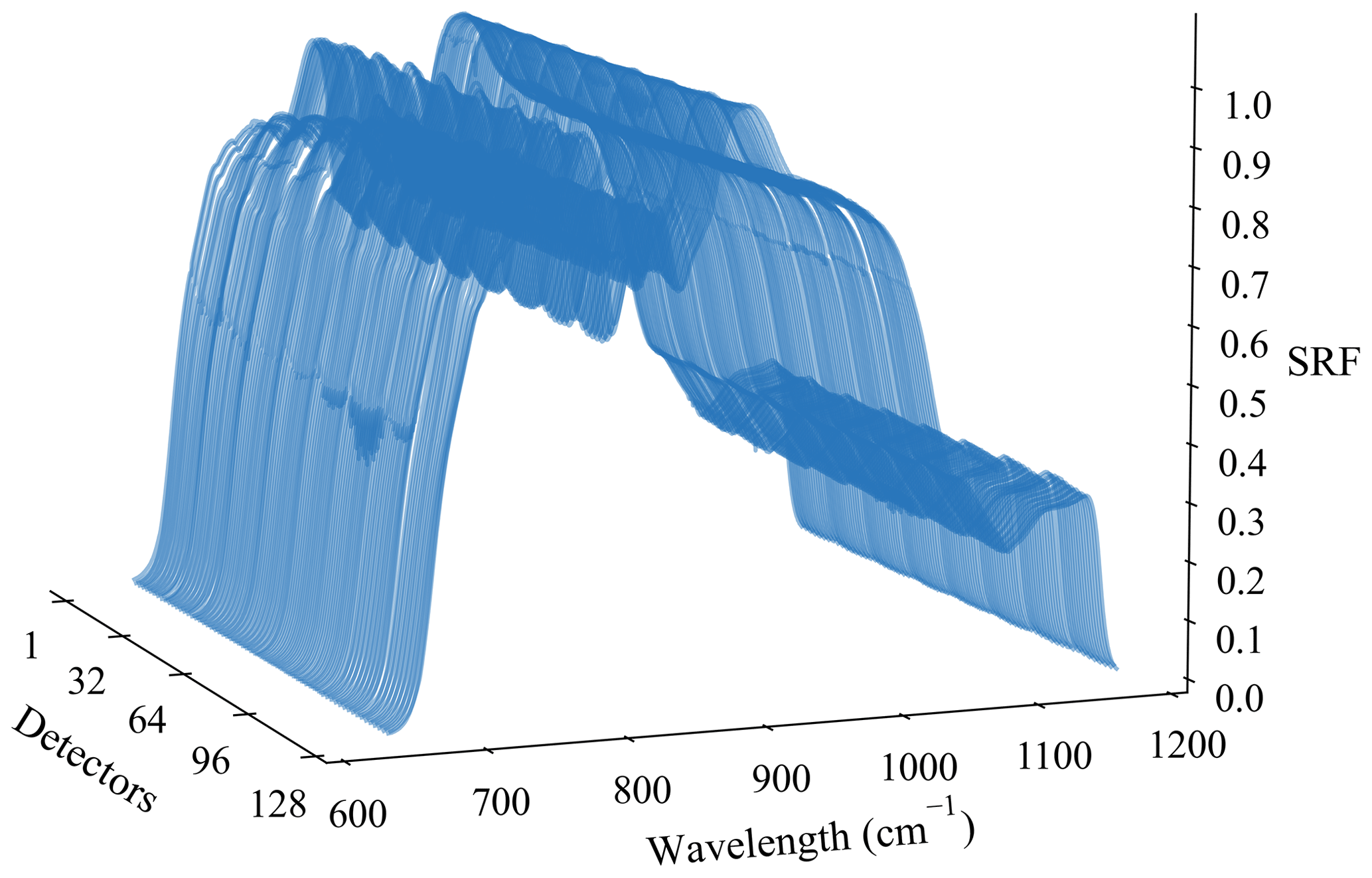
where S(ν) is the DN of the whole-band spectrum received by the detector, which is calculated from the DFT of the interferogram, and I₀(ν) is the theoretical BB radiance incident to the interferometer (GIIRS). Theoretically, the SRF of a certain sensor is an invariable function without any external influencing factors (i.e., irradiation from space), which is independent of the external BB source, with different temperatures for measurement. However, during the real calculations, the SRF derived from measurements of BB at lower temperatures is inaccurate due to the relatively lower signal-to-noise ratio. Therefore, in practice, instead of calculating the SRF for all measurements of external blackbodies with different temperatures from the laboratory calibration, only the mean value of those from the high-temperature (i.e., higher than 290 K) ones is selected to estimate different SRFs of the individual detectors of GIIRS, the final results of which are normalized, as shown in Fig. 6.

In general, the spectral dependencies of emissivity of both the external and the internal BB targets are almost identical to each other. For the LWIR band (680–1130 cm⁻¹) in particular, the emissivity for an individual channel increases gradually from 0.980 to 0.990, with its wavenumber increasing from 680 to 964 cm⁻¹, and then remains slightly variable around 0.990 for the remaining channels, with the larger wavenumbers in the LWIR band. However, for the MWIR band (1650–2250 cm⁻¹), the emissivities of all channels behave poorly, varying between 0.955 and 0.970, most (1716–2250 cm⁻¹) of which are even worse in the range between 0.955 and 0.960.

Figure 6 SRFs for all FY-4B/GIIRS detectors for the LWIR band.

Despite the fact that the nominal band of FY-4B/GIIRS for observation is between 700 and 1130 cm⁻¹, it can be seen from Fig. 6 that the practical band in which the radiation from targets can be viewed by GIIRS is wider than the nominal one. In order to calculate the radiance more accurate in this study, a wavenumber range of 640–1170 cm⁻¹ is chosen as the practical one, while the relative SRF of wavenumbers either less than 640 cm⁻¹ or greater than 1170 cm⁻¹ is approximately or even less than 0.01, which is small enough to be ignored. Meanwhile, in general, the SRFs of individual detectors of FY-4B/GIIRS approach each other, which implies that the spectral responsive characteristics for all the detectors are almost the same, at least within such a wide band as above.

3.2.2 NL coefficients and parameters from laboratory results

All three environmental tests (i.e., cold, normal, and hot) have been adopted to implement the complete calibration procedures before launch. The data selected are the laboratory BB-view measurements with temperatures between 180 and 320 K for all the detectors of FY-4B/GIIRS. When using a total of 21 groups of observations with different temperatures within the above range for the external BB for calculation of individual detectors, we found a large error in measurements when BB temperature is around 250 K, the exact reason for which is still unknown, and these values have been removed when the final fitting curve of a quadratic function is obtained. Meanwhile, the external BB views at seven different BB temperatures (270–310 K) were utilized to assess the calibration accuracy of the proposed NL correction method.

Since the external BB views at around 250 K are invalid, 20 different temperature measurements from the external BB were used in practice. Here, at least three external BB views at different temperatures are required to carry out one calculation of the linear and NL coefficients (i.e., a₁ and a₂). Therefore, the total possible number of temperature combinations for these calculations is $\sum _{x=\mathrm{3}}^{\mathrm{20}}{C}_{\mathrm{20}}^x=\mathrm{1}\mathrm{048}\mathrm{544}$ (note: $C_{\mathrm{20}}^x$ represents the combination of x out of 20), the huge size of which guarantees the reliability and stability of the statistical results of both the a₁ and a₂ coefficients. To illustrate the different distributions of both a₁ and a₂ for different detectors, particularly for those located in different positions in GIIRS's FOV, two typical detectors, labeled 56 and 96, which are located near the central and marginal positions, respectively, are selected (Fig. 5b). The distributions of two parameters (a₁ and a₂) with different measurements under normal temperature conditions are provided in Fig. 7.

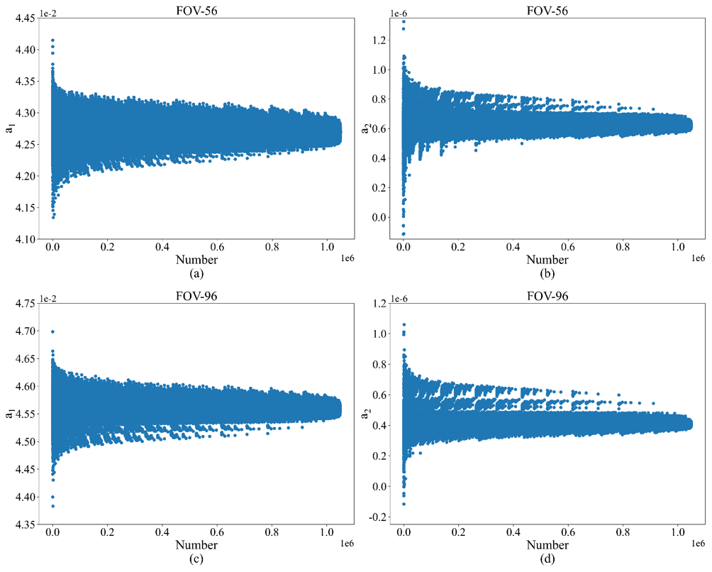
Figure 7 Typical distribution diagrams of calibration coefficients for two detectors under the normal temperature conditions: (a) the linear coefficient (a₁) of detector 56, (b) the NL coefficient (a₂) of detector 56, (c) the linear coefficient (a₁) of detector 96, and (d) the NL coefficient (a₂) of detector 96.

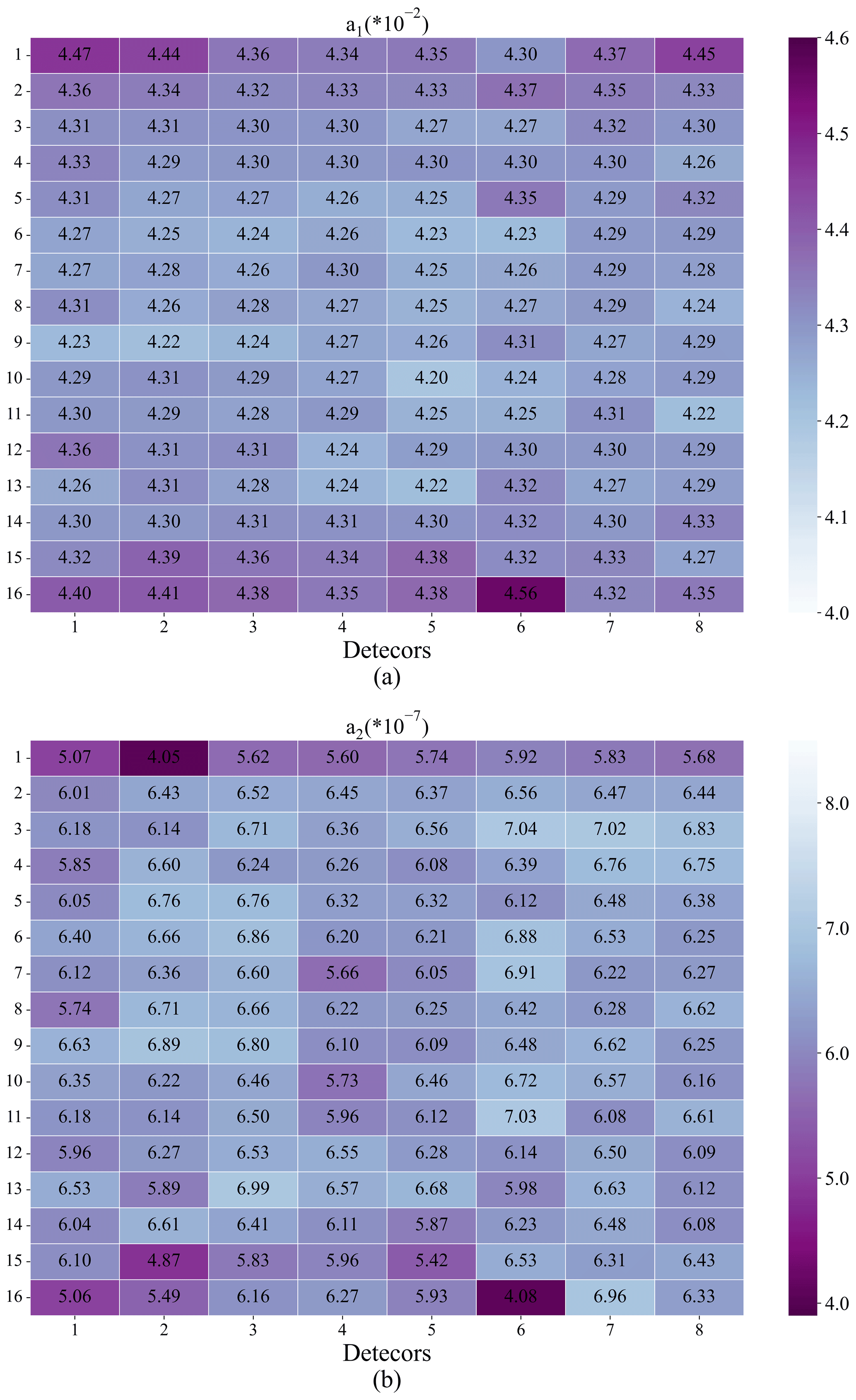
Figure 8 Mean values of the linear and the NL coefficients for all FY-4B/GIIRS detectors under the normal situation: (a) the linear coefficient (a₁) and (b) the NL coefficient (a₂).

As indicated in Fig. 7, both the linear and the NL coefficients for the two typical detectors nearly conform to a normal distribution, and their averaged linear coefficients (a₁) are $\mathrm{4.27}\times {\mathrm{10}}^{-\mathrm{2}}$ (detector 56) and $\mathrm{4.56}\times {\mathrm{10}}^{-\mathrm{2}}$ (detector 96), respectively, while those of the quadratic NL coefficients (a₂) are $\mathrm{6.22}\times {\mathrm{10}}^{-\mathrm{7}}$ (56) and $\mathrm{4.08}\times {\mathrm{10}}^{-\mathrm{7}}$ (96), respectively. Moreover, the mean values of the two coefficients (a₁ and a₂) for all the FY-4B/GIIRS detectors are also provided and shown in different colors in Fig. 8. In general, the values of the linear coefficient (a₁) for the central detectors are smaller than those for the marginal ones, the maximal relative differences of which are slightly less than 10 %. However, in Fig. 8b, the values of the NL coefficient (a₂) for marginal detectors are generally smaller (by about 50 %) than those near the center of the FOV, the main reason for which is possibly caused by the overestimated linear coefficients of the marginal ones due to the smaller amount of incident radiation, making the estimated value of the linear part too large and further leading to the calculated NL part being much smaller than the actual one (namely, the significantly smaller NL coefficients).

Table 4 Radiometric responsive characteristics of three FY-4B/GIIRS detectors located at two typical positions under different working conditions.

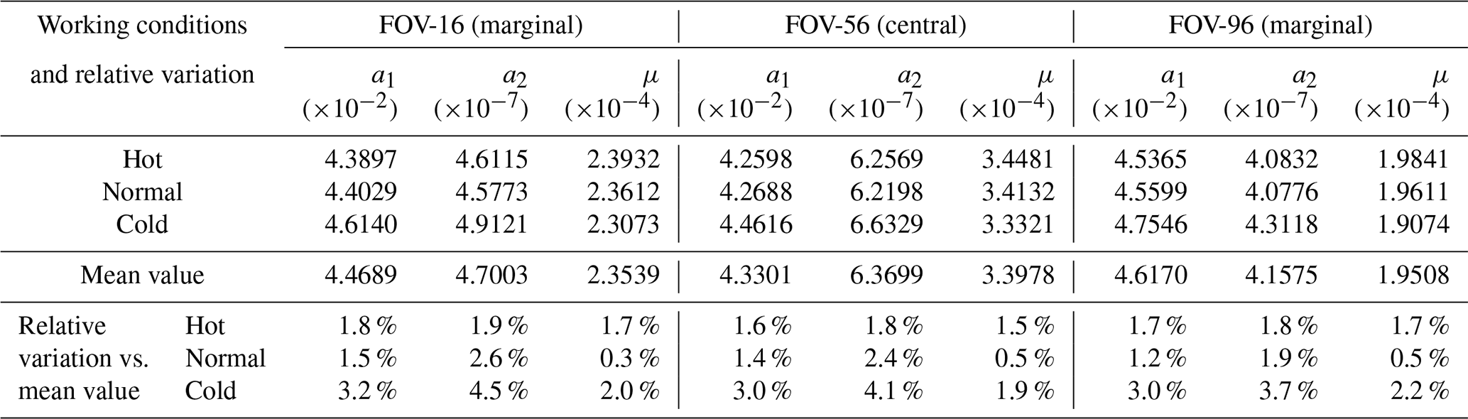
The main radiometric responsive characteristics (i.e., a₁, a₂, and μ) of FY-4B/GIIRS under three working conditions are listed in Table 4 for detectors located at two typical positions (namely, marginal and central). In general, for FY-4B/GIIRS, its linear (a₁) and NL (a₂) coefficients indeed vary significantly under different working conditions, although temperatures for both detector operation and aft optics remain stable, while the relative variations in a₂ are always larger than those in a₁ particularly for cold conditions. Moreover, the μ parameter established in the proposed NL correction method appears more stable than both a₁ and a₂, especially under normal and cold conditions. This is the main technical reason why the μ parameter is introduced in our method with an iterative algorithm: to achieve an NL coefficient (a₂) with higher accuracy.

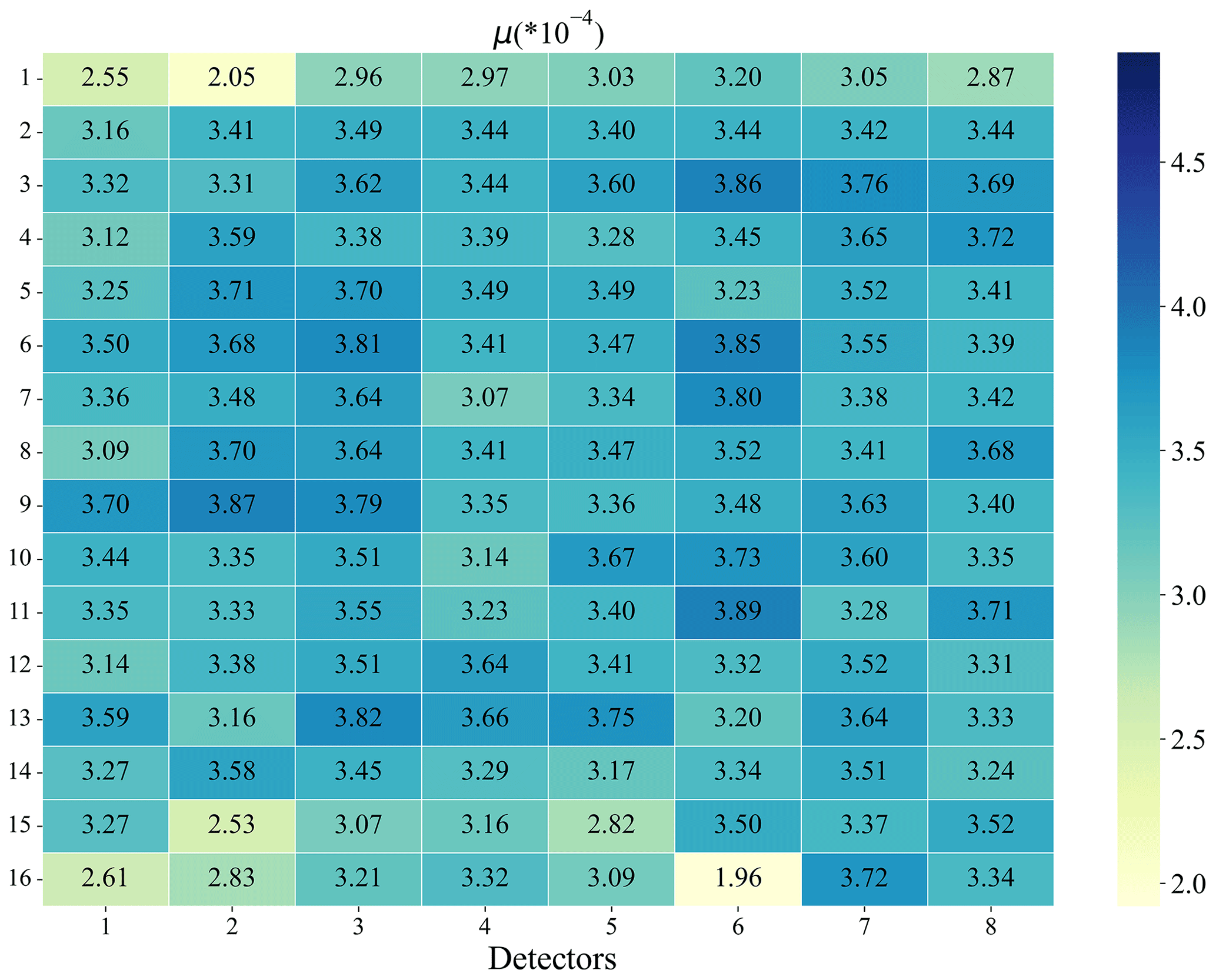
Such results indicate that μ can be regarded as a parameter that can characterize the NL response characteristics of GIIRS, which is generally invariable in different situations, particularly for different temperature configurations of the main optics. In this sense, the NL parameter (μ) of each GIIRS detector, as shown in Fig. 9, can represent the mean values for different situations. Similarly, compared to detectors near the central FOV positions, the NL parameters (μ) of the marginal ones are apparently underestimated by around 50 % versus the central ones, which is also mainly caused by their bigger linear coefficients. In fact, due to the relatively lower optical efficiency at the locations near the marginal FOV areas, the linear coefficients are usually the inverse of responsive, so the linear coefficients of the marginal ones are larger than those of the central ones. It implies that the radiometric responsiveness of the marginal detectors is generally lower, which can further lead to the smaller NL parameters (μ) even for the same detectors.

Figure 9 NL parameter (μ) for all the FY-4B/GIIRS detectors.

3.3 Preliminary assessments of different NL correction implementations with laboratory results

3.3.1 Performance comparison among three different NL correction methods

To evaluate the real performance of three different NL correction methods (i.e., the proposed one with iteration, the proposed one without iteration, and the classical NL one) during the laboratory calibration procedure, the ordinary two-point calibration mode (i.e., the hot point for the external hot BB target and the cold point for the deep space one) is adopted where the external hot BB with temperatures of 270, 280, 290, 295, 300, 305, and 310 K and the external cold BB with a temperature of 80 K (note: this is regarded as the deep space target in the infrared band) are selected to achieve two goals: one is to calculate the NL parameters (μ) with the proposed method described in Sect. 2.2 for all the GIIRS detectors, which are adopted together with measurements of the internal hot BB target to carry out a practical calibration procedure with the new developed iterative algorithm. The other goal is to provide a reference (i.e., the net radiance from the external hot BB target by subtracting the cold BB observation from the hot external BB one) to assess the calibration performance, which should be of the highest accuracy for evaluation. It should be mentioned that such a practical calibration as above, using the internal hot BB target with the derived NL parameters, is fully identical to that under in-orbit conditions. In particular, in this laboratory test of FY-4B/GIIRS, the temperature of the internal hot BB target can be set to 300, 305, 310, 315, and 320 K as required. Therefore, for the proposed NL correction method, the related calibration coefficients and iteration information are also provided in Table 5.

For the classical method, after the NL coefficient (b₂) is obtained, the interferogram (namely, output DNs from GIIRS when observing interfering radiance) can be NL corrected, and the spectrum after DFT can be further linearly calibrated with the internal hot BB target channel by channel. However, the NL coefficients of the classical method (b₂ for the interferogram and linear coefficient for each channel) are different from those of the proposed one and cannot be compared to each other directly. Therefore, some additional derivations are included as shown in Eq. (20), the results of which can help to compare the calibration coefficients between the classical and the proposed ones. Since the ideal DN (DN_ia) given by Eq. (15) has a linear relationship with incident radiance, the calibration equation between incident radiance and the output DN is satisfied by

$$\begin{array}{}\text{(20)}& \begin{array}{rl}{I}_{\mathrm{r}}& =c_{\mathrm{1}}\cdot {\mathrm{DN}}_{\mathrm{ia}}=\left[c_{\mathrm{1}}\left(\mathrm{1}+\mathrm{2}{b}_{\mathrm{2}}{\mathrm{DN}}_{\mathrm{md}}\right)\right]\cdot {\mathrm{DN}}_{\mathrm{ma}}+\left(c_{\mathrm{1}}{b}_{\mathrm{2}}\right)\\ & \cdot {\mathrm{DN}}_{\mathrm{ma}}^{\mathrm{2}}\triangleq a_{\mathrm{1}}^{{}^{\prime }}\cdot {\mathrm{DN}}_{\mathrm{ma}}+a_{\mathrm{2}}^{{}^{\prime }}\cdot {\mathrm{DN}}_{\mathrm{ma}}^{\mathrm{2}},\end{array}\end{array}$$

where I_r is the theoretical value of interfered net radiance for the internal hot BB target at different temperatures, c₁ is the linear coefficient calculated by the two-point (BB and cold space) calibration method, and b₂ is considered a constant (Han, 2018). The resulting linear and NL calibration coefficients are listed in Table 5, with respect to the internal hot BB target at different temperatures between 300 and 320 K in 5 K intervals.

Moreover, the difference between the actual BT and the calibrated one from both the classical and the proposed methods is used to represent the calibration accuracy for the interfering radiance within a wide band (i.e., 640–1170 cm⁻¹). Here, the averaged absolute difference in BT at a reference temperature (note – 305 K is usual) is

$$\begin{array}{}\text{(21)}& \mathrm{\Delta }\mathrm{BT}\left(T_{\mathrm{i}}\right)=\mathrm{|}{\mathrm{BT}}_{\mathrm{cal}}\left(T_{\mathrm{i}},T_{\mathrm{r}}\right)-{\mathrm{BT}}_{\mathrm{a}}\left(T_{\mathrm{i}},T_{\mathrm{r}}\right)\mathrm{|},\end{array}$$

where T_i is the temperature of the internal hot BB for calibration and BT_cal(T_i,T_r) is the calculated BT of the referenced external hot BB target at different temperatures (T_r) for calibration, while BT_a(T_i,T_r) is the actual BT with respect to the referenced one during laboratory calibration. Thus, the calibration results, including the linear and the NL coefficients; the calibrated BT difference (ΔBT) at the reference temperature, 305 K (i.e., T_r=305 K); and the NL parameter μ for the classical method with the internal hot BB at different temperatures, which is utilized to implement a practical in-orbit calibration, are listed in Table 5. In particular, according to Eqs. (1), (13) and (20), the deduced NL parameter (μ) with an internal hot BB target of different temperatures for the classical method is estimated for comparison.

Table 5 Comparison of the main results among three different NL correction methods.

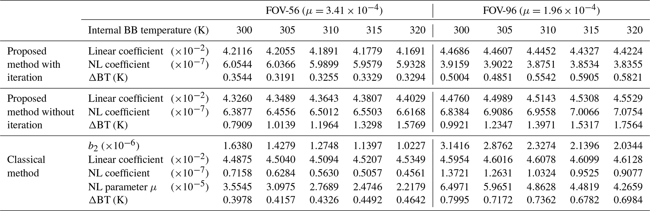
For the normal situation of FY-4B/GIIRS in the laboratory calibration using measurements of the internal hot BB target with different temperatures (i.e., 300, 305, 310, 315, and 300 K), the accurate calibration results (including linear and NL coefficients, the NL parameter, and ΔBT) of two typical detectors (i.e., detector 56 for the central one and 96 for the marginal one) are quantitatively analyzed using three different NL correction methods. Therefore, based on Table 5, several preliminary conclusions can be drawn. Firstly, for the proposed method with iteration, the linear coefficients (a₁, the most important contributor to calibration accuracy; the mean values for detectors 56 and 96 are 4.1906 and 4.4459) with the internal hot BB target at different temperatures from 300 to 320 K vibrate slightly around their mean values, the maximal relative error in which is less than 0.5 %. At the same time, the derived NL coefficients (a₂, the mean values for detectors 56 and 96 are 5.9943 and 3.8764) also perform well, with the maximal relative error around 1 %. Thereafter, the corresponding BT differences (ΔBT) are generally 0.3–0.4 K for detector 56 and 0.5–0.6 K for 96. Secondly, for the proposed method without iteration, however, the linear coefficients become bigger and bigger with increasing internal BB temperature for calibration for both detectors (56 and 96), the main reason for which is the greater NL influence on a₁ from the higher-temperature BB for calibration that makes the NL coefficients (a₂) enlarged further with a constant μ parameter. Without iteration, the final ΔBT values of this method become too big (around 1.6–1.8 for 320 K BB) to be acceptable. Thirdly, for the classical method, the situations are relatively complex. In particular, since b₂ is the NL coefficient used to describe the NL relationship between the measured DN and the ideal one, it should, at least in theory, remain nearly unchanged with respect to the internal BB target for calibration at different temperatures. However, as shown in Table 5, b₂ values are significantly dependent on BB temperature for calibration, namely, bigger b₂ is related to lower temperatures of the internal BB. Such results imply that the derived b₂ values from the classical method are inaccurate. According to Eq. (20), when the two-point method is adopted to calibrate the interfering radiance or interferogram, the gradual increase in linear coefficients (a₁^′) and decrease in NL coefficients (a₂^′) are inevitable, as seen in Table 5. Furthermore, the corresponding ΔBTs of the classical method are a bit larger than those of the proposed one with iteration (by 0.1–0.2 K). From the perspective of NL correction, the NL characteristics of GIIRS are underestimated by the classical method, the averaged $\stackrel{\mathrm{‾}}{\mathit{\mu }}$ values (i.e., $\mathrm{2.82}\times {\mathrm{10}}^{-\mathrm{5}}$ for detector 56 and $\mathrm{5.21}\times {\mathrm{10}}^{-\mathrm{5}}$ for 96) of which are 1 or 0.5 orders of magnitude smaller than their true ones (i.e., $\mathrm{3.41}\times {\mathrm{10}}^{-\mathrm{4}}$ for detector 56 and $\mathrm{1.96}\times {\mathrm{10}}^{-\mathrm{4}}$ for 96).

3.3.2 Preliminary assessments of the proposed NL correction method

Based on Sect. 3.3.1, since the ordinary temperature of the internal hot BB target is set to 305 K, more assessments of the proposed NL correction method with this internal BB for all the FY-4B/GIIRS detectors are provided in detail, particularly ΔBT values of both the interfering radiance within a wide band (640–1170 cm⁻¹) and the spectral radiance at each channel, with a resolution of 0.625 cm⁻¹ at different reference temperatures (i.e., 270, 280, 290, 295, 300, 305, and 310 K).

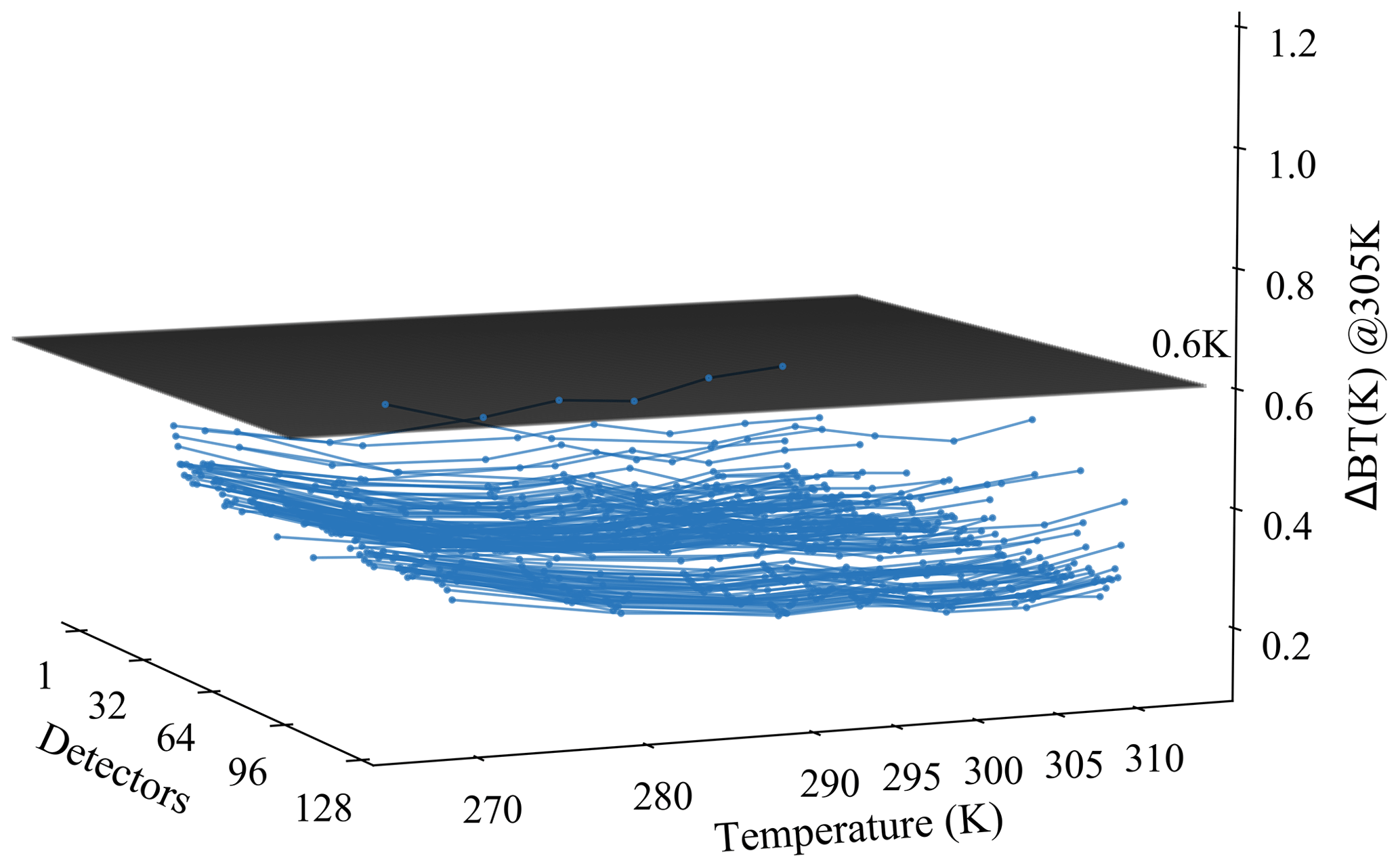
Using the proposed NL correction method, ΔBT values of the interfering radiance for all the FY-4B/GIIRS detectors are provided in Fig. 10, which are almost all less than 0.6 K at different reference temperatures between 270 and 310 K. In general, the mean ΔBT values at the reference temperatures above are around 0.3 K, except for at the relatively lower temperature of 270 K with its mean ΔBT of about 0.4 K. In particular, for some detectors located near the marginal FOV areas (i.e., the 1st, 16th, 96th, 113th, and 128th, as shown in Fig. 5), parts of their ΔBT values are even larger than 0.5 K.

Figure 10 ΔBT of interfering radiance for all the FY-4B/GIIRS detectors.

In addition, to assess the proposed NL correction method for the hyperspectral measurements from FY-4B/GIIRS in a way that is identical to that of in-orbit radiometric calibration using the onboard internal BB target, more analyzed ΔBT values under different conditions are plotted in Fig. 11. As expected, the ΔBT values without the NL correction are larger than 0.7 K for all the detectors and all the channels, as shown in Fig. 11a, which fully indicates the importance of NL correction for a GIIRS-like sensor with high accuracy requirements (i.e., usually better than 0.5 K) for observations. Correspondingly, the ΔBT values with the proposed NL correction for each detector and each channel are provided in Fig. 11b–d at different reference temperatures (305, 270, and 310 K), respectively. In particular, there are two thresholds represented by two translucent black planes for the three panels above, where the smaller ones (i.e., 0.4 K for Fig. 11b and d and 0.5 K for Fig. 11c) refer to the maximal ΔBT for the valid spectral range of 680–1130 cm⁻¹, while the larger ones (i.e., 0.7 K for Fig. 11b and d and 0.8 K for Fig. 11c) refer to the real spectral range of 640–1170 cm⁻¹. Obviously, for some marginal areas (for example less than 680 cm⁻¹ and more than 1130 cm⁻¹) of the observable spectrum, the ΔBT values behave as though they were significantly larger due to the relatively lower optical efficiency of GIIRS. On the other hand, for the lower reference temperature (i.e., 270 K compared to 305 and 310 K), the ΔBT values are a bit larger, the main reason for which is the typical NL relationship of measurement described in different radiometric units (namely, between radiance and BT) within the infrared band. Nevertheless, at the ordinary reference temperature of 305 K, the mean ΔBT values for most detectors for all the valid channels within the valid spectral range of 680–1130 cm⁻¹ are usually around 0.2–0.3 K, which is suitable for most common applications.

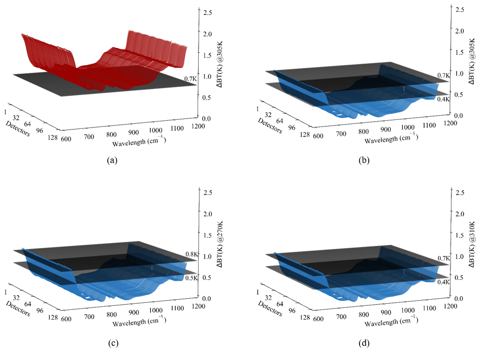
Figure 11 ΔBT of spectral radiance within each channel (with a spectral resolution of 0.625 cm⁻¹) for all FY-4B/GIIRS detectors before or after NL correction: (a) before NL correction at 305 K, (b) after NL correction at 305 K, (c) after NL correction at 270 K, and (d) after NL correction at 310 K.

4 Discussion

4.1 SRF variation under in-orbit conditions

In the proposed method, the basic roadmap of NL correction for an FTS (i.e., GIIRS) is clearly established, where the broadband interfering radiance (interferogram) with respect to the external BB at different temperatures is selected to construct an overdetermined set of equations to calculate the linear and NL coefficients, and the NL parameter μ, independent of different working conditions (i.e., different temperatures for optical and mechanical components of the sensor), is further derived to implement the NL correction during a practical in-orbit calibration using the two-point method. In particular, the NL parameter μ is regarded as a constant that is determined before launch and applied after launch. However, due to some possible causes (i.e., ice contamination) that are not totally understood (Guo and Feng, 2017), the SRF of GIIRS may have been affected to a certain extent since it was launched. Apparently, one cannot assume that the NL parameter μ of GIIRS is currently identical to that before launch. Therefore, some additional processing (i.e., in-orbit SRF modification) is needed before such a proposed method can be practical for implementation.

4.2 The non-ideal onboard BB source

An internal BB target with a temperature of 305 K is adopted to implement the two-point calibration, which is identical to that under in-orbit conditions, and the same temperature (305 K) is also selected for reference to assess the NL correction performance. The theoretical value of ΔBT should be approaching zero, and in practice ΔBT should be satisfied with 0.2–0.3 K, but the maximum value here is less than 0.4 K, as shown in Fig. 11b. The main possible reasons come from the non-ideal characteristics of the adopted internal BB target with emissivity much less than 1 (i.e., 0.97–0.99 within the spectral range of 640–1170 cm⁻¹). In fact, under such a situation, the observed radiance from such an internal BB target by the detector is not merely from the BB itself; some reflected radiation from the environmental components nearby must be considered using a certain compensation algorithm (Guo et al., 2021b). However, the estimated radiometric contribution will inevitably introduce additional uncertainty of around 0.1–0.2 K (Guo et al., 2021b), which finally causes the observable radiance from such an internal BB target to be inaccurate. To validate such a conclusion, measurements from the external BB target with a temperature of 305 K are chosen for calibration where no additional radiation is required, thanks to the low-temperature environment (i.e., generally less than 110 K) in a vacuum chamber. As indicated in Fig. 12, the distribution of ΔBT values under such conditions is almost less than 0.1 K, even for the real spectral range of 640–1170 cm⁻¹. It implies that the practical performance of the proposed NL correction method is partially dependent on the adopted internal BB target for calibration, which means that higher emissivity will produce the better NL correction.

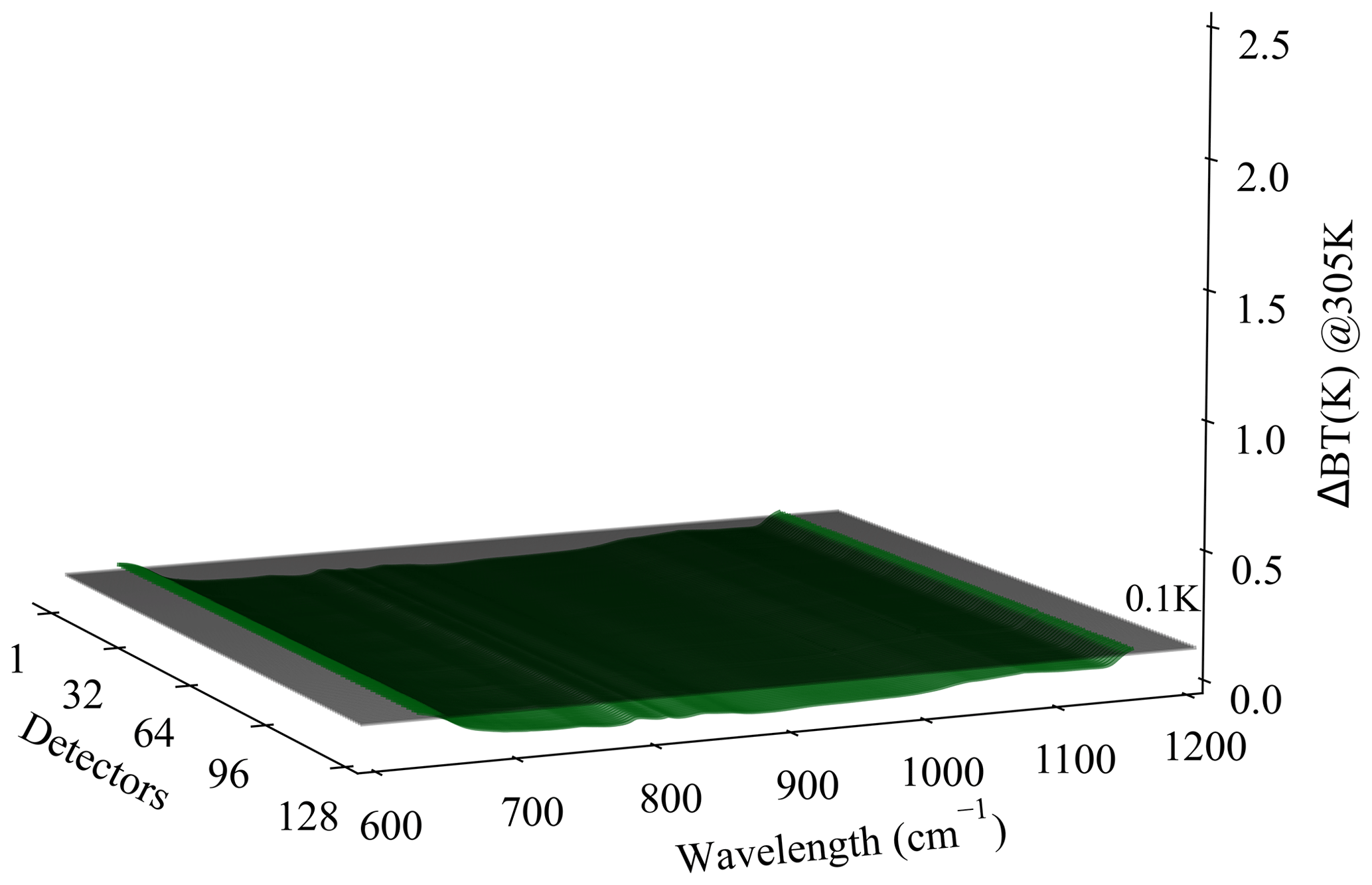
Figure 12 ΔBT of spectral radiance for all the FY-4B/GIIRS detectors and all the channels after NL correction using the external BB target.

4.3 Amplification effect of the NL coefficient on the linear one

Although the classical method of NL correction for an onboard FTS is widely applied to most similar sensors, the determined parameter b₂ cannot be absolutely accurate, a fact that depends at least on the determination of an out-of-band spectrum, which is assumed to be zero in practice. Therefore, the relationship between the linear coefficient (c₁) and the parameter b₂ can be drawn from Eq. (20) as follows,

$$\begin{array}{}\text{(22)}& \begin{array}{rl}{c}_{\mathrm{1}}& ={\displaystyle \frac{I_{\mathrm{r}}}{\left(\mathrm{2}{\mathrm{DN}}_{\mathrm{md}}{\mathrm{DN}}_{\mathrm{ma}}+{\mathrm{DN}}_{\mathrm{ma}}^{\mathrm{2}}\right)b_{\mathrm{2}}+{\mathrm{DN}}_{\mathrm{ma}}}}\\ & \approx {\displaystyle \frac{I_{\mathrm{r}}/\left(\mathrm{2}{\mathrm{DN}}_{\mathrm{md}}{\mathrm{DN}}_{\mathrm{ma}}+{\mathrm{DN}}_{\mathrm{ma}}^{\mathrm{2}}\right)}{b_{\mathrm{2}}}}.\end{array}\end{array}$$

In Eq. (22), the product of c₁ and b₂ approaches a constant, which means that the relative errors for both c₁ and b₂ are comparable. For example, a 1 % relative error in b₂ will cause around a 1 % relative error in c₁, the latter of which will introduce a bigger calibration error than the former does. Such a conclusion can be partially validated by the results listed in Table 5. Possibly, this conclusion is the main deficiency of the classical NL correction method for an FTS.

5 Conclusions

NL correction is a critical procedure to guarantee that the calibration accuracy of a spaceborne sensor approaches a reasonable level. In this study, a new NL correction method for an onboard FTS is proposed. The NL correction is directly applied to the interfered broadband radiance observed by a spaceborne FTS (i.e., GIIRS). During prelaunch laboratory calibration, NL coefficients can be calculated by fitting the theoretical received radiance and the maximal DN at absolute ZPD to different temperatures using the least-squares method. Finally, the NL parameter μ describing the relationship between the linear and NL coefficients above is determined, which is utilized to implement NL correction of an FTS (i.e., GIIRS) together with the inaccurate linear coefficient from the two-point calibration method. In addition, the NL parameter μ is almost independent of different working conditions and can be applied directly while in orbit. Moreover, to overcome the inaccurate linear coefficient, which is inevitably affected by the NL response of the sensor and has an impact on the NL correction, an iteration algorithm is established to make the linear and the NL coefficients converge to their stable values, with relative errors of less than 0.5 % and 1 %, respectively, which is universally suitable for NL correction of both infrared and microwave sensors.

Using an onboard internal BB that is identical to the in-orbit calibration, the final calibration accuracy for all the detectors and all the channels using the proposed NL correction method is validated as around 0.2–0.3 K at an ordinary reference temperature of 305 K. Significantly, the relative error in the classical method in the NL parameter that immediately transmits to the linear one and in theory inevitably introduces some additional errors around 0.1–0.2 K (for the interfering radiance) no longer exists. Moreover, the adopted internal BB with the higher emissivity will produce the better NL correction performance in practice.

In the future work, the adopted internal BB with higher emissivity will produce the better NL correction performance in practice. The proposed NL correction method is scheduled for implementation on GIIRS on board the FY-4A satellite and on board its successor, after modifying the possible SRF variations. Moreover, the real measurements from GIIRS after NL correction can be inter-calibrated with those of a reference sensor, i.e., the Infrared Atmospheric Sounding Interferometer (IASI) or CrIS, to validate its calibration accuracy after NL correction.