The Far-INfrarEd Spectrometer for Surface Emissivity (FINESSE) – Part 1: Instrument description and level 1 radiances

The Far-INfrarEd Spectrometer for Surface Emissivity (FINESSE) instrument combines a commercial Bruker EM27 spectrometer with a front-end viewing and calibration rig developed at Imperial College London. FINESSE is specifically designed to enable accurate measurements of surface emissivity, covering the range 400–1600 cm⁻¹, and, as part of this remit, can obtain views over the full 360° angular range.

In this part, Part 1, we describe the system configuration, outlining the instrument spectral characteristics, our data acquisition methodology, and the calibration strategy. As part of the process, we evaluate the stability of the system, including the impact of knowledge of blackbody (BB) target emissivity and temperature. We also establish a numerical description of the instrument line shape (ILS), which shows strong frequency-dependent asymmetry. We demonstrate why it is important to account for these effects by assessing their impact on the overall uncertainty budget on the level 1 radiance products from FINESSE. Initial comparisons of observed spectra with simulations show encouraging performance given the uncertainty budget.

1 Introduction

The infrared spectral emissivity of the Earth's various surface types plays a fundamental role in determining their radiative emission, influencing the surface energy budget and the efficiency with which the Earth cools to space. Knowledge of infrared surface emissivity, including any angular dependence, is also a prerequisite for satellite instruments exploiting these wavelengths to retrieve surface and lower tropospheric temperatures and/or profile concentrations of certain atmospheric constituents.

Recent modelling work has also indicated that surface emissivity in the far-infrared (wavelengths longer than 15 µm) may play a more important role than previously thought in influencing, in particular, high-latitude surface temperature and its evolution (Feldman et al., 2014; Huang et al., 2018). Typically, surface emission at these wavelengths is attenuated by strong water vapour absorption. However, under clear skies at low water vapour concentrations absorption, micro-windows within the far-infrared can open, allowing the surface emission to propagate further through the atmosphere and, under certain conditions, escape to space.

To date, very few retrievals of far-infrared emissivity exist. Those that do tend to have been obtained over a limited area or for a limited time (e.g. Bellisario et al., 2017; Palchetti et al., 2021; Borbas et al., 2021). This will change with the launch of two new satellite missions, the Polar Radiant Energy in the Far-Infrared Experiment (PREFIRE) (L'Ecuyer et al., 2021) and the Far-Infrared Outgoing Radiation Understanding and Monitoring (FORUM) missions (Palchetti et al., 2020). Looking further ahead, there are also plans to fly a far-infrared instrument as part of NASA's Atmosphere Observing System mission (Blanchet et al., 2011; Libois et al., 2016).

Theoretical studies suggest that both PREFIRE and FORUM will be capable of retrieving surface emissivity across both mid- and far-infrared under certain conditions (Ben-Yami et al., 2022; Xie et al., 2022). These findings reinforce results obtained from high-altitude aircraft flights over the Greenland plateau (Murray et al., 2020) and, combined with the proliferation of far-infrared-focused missions, imply a need for the development of ground-truthing capability to verify retrievals made across the infrared.

This need has motivated the development of the Far-INfrarEd Spectrometer for Surface Emissivity (FINESSE). Combining a commercial Bruker EM27 spectrometer with a custom-built front-end pointing and calibration system, the instrument is portable and can be deployed to different locations as required. Its particular innovation is the ability to point through a full 360° range, negating the need to tilt the instrument to avoid its own footprint and allowing the angular dependence of emissivity to be easily assessed.

In the sections that follow, we describe the various components of FINESSE and discuss how it has been characterized. Particular attention is paid to the calibration procedure and assessment of the instrument line shape (ILS), and we show how knowledge of these parameters flows through to the ultimate uncertainty budget associated with the level 1 radiance products. Characterization of this uncertainty budget is particularly important when using the FINESSE measurements to infer surface emissivity, a process which we describe in full in the accompanying part, Part 2 (Warwick et al., 2024).

2 System description

2.1 EM27 spectrometer

The EM27 is a relatively inexpensive ruggedized spectrometer using a RockSolid™ pendulum interferometer, with low sensitivity to mechanical shocks and vibrations, which has been hardened for operation in temperatures as low as 253 K. EM27 spectrometers are primarily designed for real-time remote monitoring of atmospheric chemical concentrations but have also been used to undertake surface emissivity measurements in the mid-infrared from 700–2200 cm⁻¹ (e.g. Langsdale et al., 2020).

The EM27 series is configurable, with the choice of beam splitter and detector determining the spectral range that can be covered. It can be used in either active mode, utilizing a background source, or passive mode, observing ambient atmospheric or target radiance. To extend measurements into the far-infrared, FINESSE uses a combination of a potassium bromide (KBr) beam splitter, an extended mercury cadmium telluride (MCT) detector cooled to 77 K using liquid nitrogen, and a diamond input window for the interferometer housing. Combined, these components give spectral coverage from 400–1600 cm⁻¹. As KBr is hygroscopic, the interferometer housing is hermetically isolated from ambient conditions by the diamond input window and kept dry using a desiccant, with typical enclosure humidity kept below 3 %. The use of an extended MCT detector gives greater sensitivity than uncooled deuterated L-alanine doped triglycene sulfate (DLaTGS) detectors at wavenumbers greater than 450 cm⁻¹ and facilitates a more rapid measurement cycle. This latter advantage is important if ambient conditions are fluctuating rapidly with time. The disadvantage is the need to source and perform repeated fills of liquid N₂ during extended operations. The resolution of the instrument can be set using the control software supplied with the EM27 at values between 0.5 and 4 cm⁻¹.

As built, the EM27 has a single variable-temperature blackbody (BB) calibration target, which is internal to the interferometer enclosure. During typical operation, this blackbody is used on a periodic basis, approximately every 2 h, to provide a nominal radiance calibration for the observations. When in calibration mode, an internal mirror is rotated into the beam path, bringing the blackbody into the instrument field of view. During the internal calibration, the blackbody is first cooled, and a user-selectable number of scans are acquired, after which the blackbody is heated and a similar number of scans are acquired. These two sets of observations can then be applied to external observations to yield radiance estimates. For our scientific goals, we desire a verifiable accuracy assessment so we use purpose-built external blackbody targets (Sect. 2.2) to provide calibration for FINESSE. However, we find it helpful to initiate an internal calibration at the start of the day: this sets the internal calibration target at 343 K, providing a thermal heat source for the system in cold environments. Additionally, as described in Sect. 3.5, a comparison of the spectral response functions derived from the external and internal calibration targets is used to derive the frequency-dependent instrument line shape.

2.2 FINESSE front-end scene selection and calibration system

As described above, the standard calibration process of the EM27 does not fully account for the mirror reflectivity and the transmission of any window to the exterior. To account for this and allow more versatility in scene selection, we employ a purpose-built external targeting system, with a scene-selectable view mirror and external blackbody sources.

Figure 1 shows the EM27 and external calibration system during assembly. The steerable mirror at the front of the EM27 input aperture can be rotated through 360°. This allows us to steer the EM27 view towards the hot or ambient-temperature blackbody for calibration purposes or towards a target scene at any given angle from zenith through to nadir.

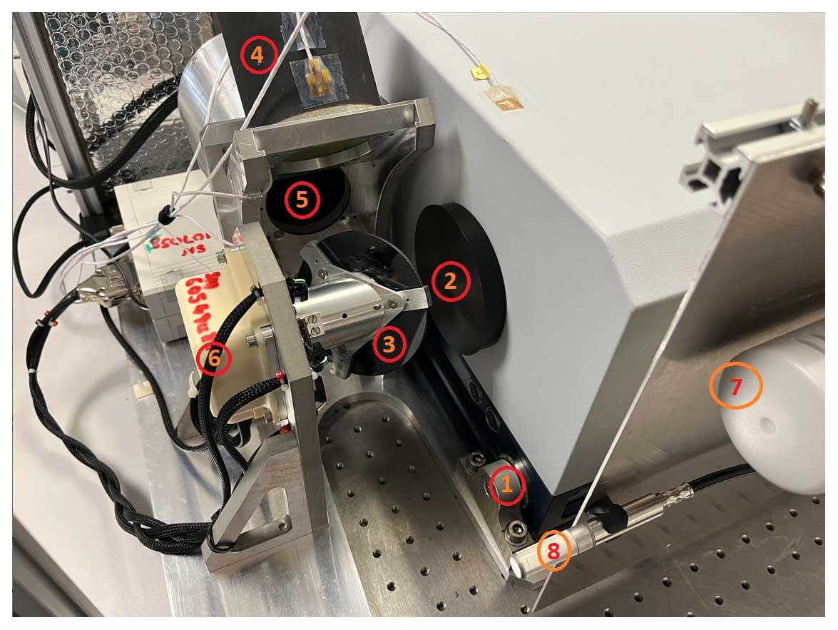
Figure 1 Close-up of the front-end pointing and calibration systems attached to the EM27. 1: dowel locator and receptacle. 2: EM27 input window. 3: steering mirror. 4: ambient temperature blackbody. 5: hot blackbody. 6: stepper motor. 7: Vaisala CO₂ monitor and 8: Vaisala pressure/humidity and temperature sensor.

The blackbody cavities are fabricated using an 80 mm outer diameter copper rod (Fig. 2a). The cavities themselves are 80 mm in depth, with high-emissivity target backplates. The inner cavity is machined to form a cone tapering towards the input aperture so that the wall thickness is 7 mm at the back of the cavity to 9 mm at the front. This design is based on heritage from the Tropospheric Airborne Fourier Transform Spectrometer, which was developed in-house at Imperial College (Canas et al., 1997).

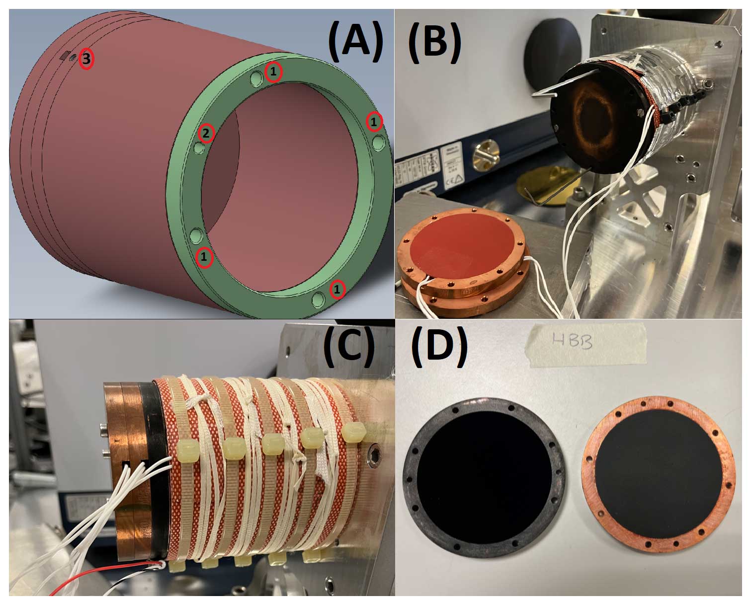
Figure 2 (a) Schematic layout of the hot blackbody. The cavity and backplates are machined from a solid copper rod that is 80 mm in diameter. The copper cavity is thermally isolated from the mounting frame using a Tufnol isolating ring (green). Holes marked with 1 indicate the locations of fixing bolts, and through hole 2; a PRT100 temperature sensor can be inserted into the front of the copper cavity, while an additional PRT100 is inserted into the backplate via hole 3 and sits central to the backplate disc 1.5 mm from the disc surface. (b) Cavity fixed to the mounting frame. To the lower-left are two additional plates which are seen bolted to the target plate in panel (c). Each plate includes a 5 W rubber heater pad whose diameter matches the diameter of the inner target plate emission surface. A 25 W heater is wrapped around the circumference of the cavity wall. Panel (d) shows target backplates; to the left is a plate coated in Vantablack and to the right a plate coated in Aeroglaze Z306.

To obtain a high effective emissivity, the cavity emission surfaces are coated in Aeroglaze Z306 paint (Adibekyan et al., 2017). The backplates sealing the blackbodies are copper discs of 7 mm in thickness: in initial testing and for the measurements of de-ionized water described in Part 2 (Warwick et al., 2024), these were also coated in Z306. For the purposes of establishing their performance and also for future use, we acquired a second set of backplates coated in Vantablack S-IR (Adams et al., 2019). To monitor the blackbody temperature and obtain information regarding any temperature gradient, we use class-A PRT100 sensors that are 25 mm × 2.8 mm in diameter: one is embedded centrally within the backplate disc 1.5 mm from the emission surface, and a second is embedded at the front end of the cavity wall (Fig. 2a). The hot blackbody cavity has an external heater pad mounted around the circumference, while the backplates use two compressible circular rubber heater pads, matching the inner-surface diameter. These pads are mounted on the far side of the disc and are each gently compressed between successive copper discs to give good thermal contact (Fig. 2c). The hot blackbody and heaters are insulated and housed in an aluminium case, isolating them from ambient conditions. Power to the heater pads is controlled using a TE Technology TC-48-20 controller with thermistor feedback, providing a nominal set point for the hot blackbody temperature of about 343 K. As is demonstrated in Sect. 3.2, shortly after the set point temperature is reached, the stability of this hot blackbody is better than 0.1 K over periods of hours.

The ambient temperature blackbody is not temperature-stabilized and is left exposed to the ambient atmospheric conditions. PRT100 sensors are embedded within the backplate and front of the cavity wall to monitor the emission and cavity wall temperatures. When using FINESSE, we have measurement periods that typically last a few hours. Once the system has stabilized after initial power up, we find that there is a warming trend in the ambient blackbody temperature due to its position relative to the hot blackbody. The magnitude of this trend is dependent on ambient conditions. In the laboratory, it is on the order of 0.03 K min⁻¹, increasing to the order of 0.1 K min⁻¹ in some deployment environments. These drifts can be accurately accounted for by extrapolation between calibration measurements as needed. Overall, the high thermal mass of the copper body helps to temporally smooth the effects of fluctuations in external conditions.

We typically operate FINESSE at a spectral resolution of 0.5 cm⁻¹, which translates to a scan time of about 1.5 s to acquire a single interferogram. To achieve an adequate signal-to-noise ratio while ensuring low impact on the calibration response from changing ambient atmospheric conditions, we set the Bruker OPUS instrument control software to acquire 40 individual interferograms for a given target view. The control of all data acquisition, target views, and system logging is performed via a custom-built FINESSE graphical user interface (GUI). This GUI connects to the EM27 through the EM27 internal PC web interface and is used to issue start/stop scan commands. To automate data acquisition, we have created script files, which are loaded into the GUI interface and define an observation sequence which is run repetitively for a given number of cycles. Typically, a calibration–observation cycle consists of three target views: a hot blackbody view, an ambient blackbody view, and a scene measurement, taking a little over 3 min to complete before the cycle is repeated.

2.3 Ancillary atmospheric measurements

In order to retrieve emissivity, the influence of the atmospheric path between the detector and the surface needs to be accounted for. To help to constrain conditions along the path ancillary measurements of atmospheric temperature, pressure and relative humidity are provided by a Vaisala PTU300 transmitter (Fig. 1). These can also be used to provide context when characterizing the instrument spectral response and assessing its stability. Quoted calibration uncertainties are within 0.05 hPa, 1 %, and 0.1 K over the ambient ranges typically observed during these observations. A separate Vaisala GMP343 probe is used to monitor CO₂ concentrations (Fig. 1). The uncertainty associated with this CO₂ sensor is quoted as 3 ppmv + 1 % of the reading at 25 °C.

3 FINESSE instrument characteristics and performance

To optimize the retrieval of emissivity from the FINESSE radiance measurements, we require either the instrument spectral response to be stable or that any drift in response be slow and measurable over the period of the radiance measurements. We also require knowledge of the FINESSE instrument line shape so that this can be accounted for in the forward modelling of the observed radiances.

The sections that follow outline our data processing strategy. These steps include the application of spectral-phase corrections required to remove instrument self-emission terms that might compromise the radiance calibration. The stability of the spectral response function is evaluated, including the impact of assumptions concerning the calibration blackbody emissivity and temperature. We also look closely at the instrument spectral line shape of the Bruker EM27 which appears to have significant frequency-dependent line broadening and line asymmetry.

3.1 Phase correction

A thorough explanation of Fourier transform spectrometry can be found in many textbooks (e.g. Griffiths and De Hasseth, 2007). In this paper, we limit details of the application of the Fourier transform to a simple formulation of the phase function and phase correction of the complex spectra in order to highlight a phase anomaly that impacts the spectra observed by the EM27.

After acquisition of the interferogram, the following complex Fourier transform (Eq. 1) is used:

$$\begin{array}{}\text{(1)}& B\left(\mathit{\sigma }\right)={\int }_{-\mathrm{\infty }}^{+\mathrm{\infty }}I\left(x\right)e^{-\mathrm{2}\mathit{\pi }i\mathit{\sigma }x}\mathrm{d}x\end{array}$$

to yield the complex spectrum (Eq. 2)

$$\begin{array}{}\text{(2)}& B\left(\mathit{\sigma }\right)=\mathit{Re}\left(\mathit{\sigma }\right)\cos \left({\mathit{\theta }}_{\mathit{\sigma }}\right)+\mathit{Im}\left(\mathit{\sigma }\right)\sin \left({\mathit{\theta }}_{\mathit{\sigma }}\right).\end{array}$$

Here, σ is the wavenumber in inverse centimetres, x is the optical path difference in centimetres, Re and Im denote the real and imaginary spectral components, and θ_σ is the wavenumber-dependent phase function.

The phase function is retrieved from a low-resolution 2.5 cm⁻¹ complex spectra; thus,

$$\begin{array}{}\text{(3)}& {\mathit{\theta }}_{\mathit{\sigma }}=\text{arctan}{\displaystyle \frac{\mathit{Im}\left(\mathit{\sigma }\right)}{\mathit{Re}\left(\mathit{\sigma }\right)}}.\end{array}$$

This phase function is applied to the full-resolution complex spectra using the method described by Mertz (1965).

In routine operations of the EM27, the OPUS control software acquires and stores, amongst additional housekeeping information, individual raw interferograms for each 1.5 s scan from which the complex spectra are obtained. When deriving the phase functions for individual spectra, we found that these phase functions exhibited features consistent with significant self-emission from the EM27. To address this, we follow an approach which properly corrects for an anomalous phase associated with instrument self-emission. To remove the influence of this anomalous phase on the phase function for individual spectra, Revercomb et al. (1988) take the difference between two complex spectra – for example, the complex spectra associated with the hot and ambient targets before the phase function is derived and applied. The same authors note that if the instrument interferogram acquisition system is stable between different scene views, differencing the interferograms before applying the phase correction will also correct for the anomalous phase. For the EM27, we find the reproducibility of the sampled interferograms between calibration cycles to be very stable and hence choose to difference the interferograms, thus removing the self-emission term, before transforming and phase-correcting.

3.2 FINESSE spectral response and spectral response stability

The instrument spectral response converts raw spectral signals to radiance and, for FINESSE, is derived from measurements of the external calibration targets; thus the following applies:

$$\begin{array}{}\text{(4)}& \begin{array}{rl}& R(\mathit{\sigma }{)}_{\mathrm{FIN}}\\ & ={\displaystyle \frac{\text{FFT}\left\{I(x{)}_{\mathrm{hot}}-I(x{)}_{\mathrm{amb}}\right\}}{\begin{array}{l}\left[{\mathit{\epsilon }}_{\mathrm{eff}}\left(\mathit{\sigma }\right)B{\left(\mathit{\sigma },T\right)}_{\mathrm{hot}}+\left(\mathrm{1}-{\mathit{\epsilon }}_{\mathrm{eff}}\left(\mathit{\sigma }\right)\right)L(\mathit{\sigma }{)}_{\mathrm{hot}}^{\mathrm{ext}}\right]-\\ \left[{\mathit{\epsilon }}_{\mathrm{eff}}\left(\mathit{\sigma }\right)B{\left(\mathit{\sigma },T\right)}_{\mathrm{amb}}+\left(\mathrm{1}-{\mathit{\epsilon }}_{\mathrm{eff}}\left(\mathit{\sigma }\right)\right)L(\mathit{\sigma }{)}_{\mathrm{amb}}^{\mathrm{ext}}\right]\end{array}}}.\end{array}\end{array}$$

The numerator is the phase-corrected complex spectrum derived from the difference in sequentially measured interferograms for the hot and ambient blackbodies. The denominator is the difference in the radiance signal from the two blackbodies, which comprises their Planckian emission, B(σ,T), modulated by the cavity effective emissivity, ε_eff, and the reflected external radiance incident on each cavity, L(σ)^ext. If the effective emissivity of the blackbody cavities is assumed to be unity, then the reflected terms disappear, and the denominator relaxes to the difference between two Planck functions.

We initially make this simplifying assumption in order to investigate the stability of the FINESSE response function under laboratory conditions. The system was configured to run a series of alternating views between the hot and ambient temperature calibration targets with a 96 s integration time for each target. After powering up, the system was given 60 min to stabilize before measurements were initiated and left to run for about 6.5 h.

Figure 3a shows the 119 spectral response functions acquired during this period as a function of wavenumber. To provide greater detail, Fig. 3b shows the spectral response in four wavenumber channels, expressed as the percentage difference relative to the channel average spectral response over the entire period. During the first 30 min, we see that the system is still stabilizing, slowly dropping to a stable behaviour from about 2 % above the average. After this initial 30 min, the stability at 500, 900, and 1200 cm⁻¹ is within 0.2 % of the mean response after stabilization. It is even possible to see when the detector dewar, housing the liquid nitrogen coolant, was topped up at 15:30 UTC. Given its proximity to the detector band edge, the 410 cm⁻¹ channel is noisier, as expected. This channel also has a discernible trend after the initial stabilization period, with a decrease in spectral response from 1 % above the mean to 1 % below. This may reflect changing atmospheric conditions (Fig. 3c) to which the 410 cm⁻¹ channel will be more susceptible. However, away from the detector band edges, the stability of the FINESSE system spectral response appears excellent.

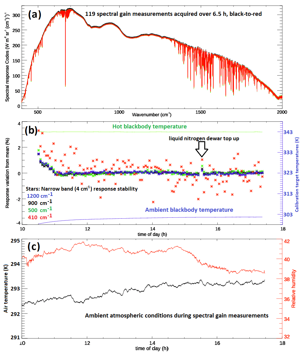
Figure 3 (a) FINESSE spectral gain function, 119 measurements, from black to red over 6.5 h; the y axis “codes” refer to the detector signal response to incident radiance. (b) Gain variance with time for four spectral channels. These channels have a width 4 cm⁻¹ and are centred on 1200, 900, 500, and 410 cm⁻¹. The solid green and purple lines show the hot and ambient blackbody temperatures. Panel (c) shows the ambient atmospheric conditions in the laboratory during the extended measurement period.

3.3 Blackbody emissivity estimates

The FINESSE blackbodies use a simple cavity geometry with a relatively low aperture-to-length aspect ratio to isolate the target backplate emission in the field of view of the instrument from the external radiance field beyond the blackbody aperture. Typically, cavities are held at the same temperature as the backplate and are designed such that rays entering the cavity undergo multiple internal reflections before being reflected into the field-of-view of the spectrometer. These multiple reflections compensate for coatings with relatively low emissivity and enhance the effective emissivity of the BB target.

As noted earlier, in our first iteration of blackbody design, both the cavity walls and the backplates of the FINESSE blackbodies are coated in Aeroglaze Z306, which has a measured emissivity of between 0.9 and 0.97, depending on wavenumber and temperature. The emissivity temperature dependence shown in previously published data suggests an increase in emissivity of about 5 % between 298 and 423 K for a surface coated in Z306 (Adibekyan et al., 2017). Linearly interpolating these published emissivity curves for Z306 with the temperature to the FINESSE blackbody temperatures of 300 and 343 K gives an anticipated difference in spectral emissivity between the blackbodies of less than 2 % (Fig. 4e).

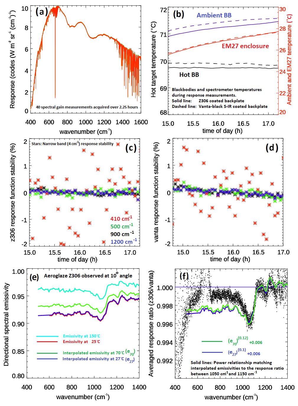
Figure 4 (a) Forty spectral response functions obtained using the full Z306 blackbodies (Z306 case). (b) Temperatures of the blackbodies and EM27 enclosure during the response function measurements: solid lines correspond to Z306 case and dashed lines to the Vanta case. (c) Response function as a function of time in four selected wavenumber channels for the Z306 case. (d) As panel (c) but for the Vanta case. (e) Emissivity measurements at a 10° view angle for Z306 for surface temperatures of 298 and 423 K (Adibekyan et al., 2017) and interpolated emissivities for temperatures associated with the FINESSE blackbodies. (f) Ratio of Z306 to Vanta spectral response. Fitted lines show the power relationships required to best match the interpolated emissivities shown in panel (e) to the step in the ratio between 1050 and 1150 cm⁻¹.

Vantablack S-IR coatings have measured emissivities in excess of 0.997 at wavenumbers greater than 700 cm⁻¹ (Adams et al., 2019), with no known emissivity temperature dependence. The choice of a Vantablack-coated blackbody is therefore theoretically preferable over one coated in Z306 and so, in a second iteration of the blackbodies, we coated both backplates with Vantablack S-IR. However, due to the fragility of Vantablack and the difficulty in coating the inner surface of the cavity, it was decided to retain the Z306 cavity coating. We make the assumption that the high emissivity of the Vantablack-coated backplate within the cavity housing will provide an effective emissivity not measurably discernible from unity for the FINESSE setup.

The measurements described in Part 2 (Warwick et al., 2024) use the fully Z306-coated blackbodies. To derive an upper limit for the effective emissivity of the blackbodies coated wholly in Z306, we compare the spectral response of the two blackbody configurations. Specifically, we measure the instrument spectral response over 2 h periods for each backplate type and undertake a comparison through the ratio of these responses, as shown in Eq. (5). We note that as the geometries of the hot and ambient blackbodies are the same, the reflected components, included in Eq. (4), will effectively cancel each other out. For the full-Z306 case, this assumes that the temperature-induced emissivity difference of 2 % will be adequately mitigated by the cavity effect.

$$\begin{array}{}\text{(5)}& \begin{array}{rl}& {\displaystyle \frac{R(\mathit{\sigma }{)}_{\mathrm{FIN}}^{\mathrm{Z}\mathrm{306}}}{R(\mathit{\sigma }{)}_{\mathrm{FIN}}^{\mathrm{Vanta}}}}=\\ & {\displaystyle \frac{\text{FFT}\left\{I(x{)}_{\mathrm{hot}}^{\mathrm{Z}\mathrm{306}}-I(x{)}_{\mathrm{amb}}^{\mathrm{Z}\mathrm{306}}\right\}{\mathit{\epsilon }}_{\mathrm{eff}}^{\mathrm{Vanta}}\left(\mathit{\sigma }\right)\left(B(\mathit{\sigma },T{)}_{\mathrm{hot}}^{\mathrm{Vanta}}-B(\mathit{\sigma },T{)}_{\mathrm{amb}}^{\mathrm{Vanta}}\right)}{\text{FFT}\left\{I(x{)}_{\mathrm{hot}}^{\mathrm{Vanta}}-I(x{)}_{\mathrm{amb}}^{\mathrm{Vanta}}\right\}{\mathit{\epsilon }}_{\mathrm{eff}}^{\mathrm{Z}\mathrm{306}}\left(\mathit{\sigma }\right)\left(B(\mathit{\sigma },T{)}_{\mathrm{hot}}^{\mathrm{Z}\mathrm{306}}-B(\mathit{\sigma },T{)}_{\mathrm{amb}}^{\mathrm{Z}\mathrm{306}}\right)}}\end{array}\end{array}$$

For both sets of observations, FINESSE was allowed to stabilize for the same amount of time, and the measurements were started with both hot and ambient blackbodies at similar temperatures (Fig. 4b). In both cases, FINESSE was configured to run a series of alternating views of 96 s in duration between the hot and ambient-temperature calibration targets. Figure 4a displays the 40 spectral responses using the wholly Z306 setup acquired over this time. Panels (c) and (d) show the stability of the spectral response function in four selected narrow band channels of 4 cm⁻¹ in width centred on 410, 500, 900, and 1200 cm⁻¹. The stability of the response function during the Z306 backplate measurements is compatible with that shown in Fig. 3, within 0.2 % of the mean for the 500, 900, and 1200 cm⁻¹ channels, with a small negative trend over the measurement period of about 0.1 % (Fig. 4c). Similarly to Fig. 3b, the 410 cm⁻¹ band shows a much higher scatter associated with higher noise at the edges of the detector response, accompanied by a slight increase over the 2 h period. For the Vanta backplate case, similar behaviour is seen in the 500, 900, and 1200 cm⁻¹ channels, with all of them showing a small negative drift in the response function of about 0.4 % over the 2 h period. There is significantly less scatter in the 410 cm⁻¹ channel for the Vanta case than is seen for the Z306 measurement, but there is a decrease in the relative response with time. Overall, the stability of the system is demonstrably excellent across much of the FINESSE spectral range, allowing us to estimate the effectiveness of the cavity using the known spectral structure of Z306.

Our comparison of the Z306 and Vanta spectral response functions is shown in Fig. 4f. The spectral behaviour outside of regions of strong atmospheric absorption from water vapour and CO₂ shows a clear signature related to the spectral emissivity of Z306. To highlight this, we have applied a power relationship and offset to the interpolated Z306 emissivities shown in Fig. 4e to match the step seen between 1050 and 1150 cm⁻¹ in the spectral response ratio. The step in our interpolated emissivity is 0.04 at 300 K and 0.03 at 343 K, while the equivalent step in the FINESSE spectral response ratio is 0.004 (Fig. 4f), which is a significant improvement suggesting a cavity enhancement on the order of 8.

The direct comparison of the ratio between the Z306 and Vantablack cases shown in Fig. 4f would suggest an effective emissivity for the cavities with Z306-coated backplates of better than 0.998 across the majority of the FINESSE spectral range, excluding the band between 1050 and 1150 cm⁻¹, where the values drop to a minimum of 0.996. Between 400 and 500 cm⁻¹, we see a large divergence in the response function ratio. This is most likely due to the proximity of these wavelengths to the detector band edge combined with the effect of drifts in the ambient atmospheric state. For our analysis and calibration purposes, we use the inferred emissivity of 0.998 at 500 cm⁻¹ at lower wavenumbers.

We expect that the 0.4 % drift we see in spectral response for the Vanta case (Fig. 4d) coupled with our assumption that, for the Z306 case, the reflected radiance signals from the ambient and hot blackbodies cancel each other out, will introduce some uncertainty in our effective emissivity estimate. By treating the 0.4 % drift as an uncertainty and adding, in quadrature, a 0.25 % uncertainty to account for the 2 % emissivity offset for the Z306 targets at 300 and 343 K, we estimate an overall uncertainty in the effective emissivity of 0.005.

3.4 Knowledge of BB emission temperature

There are three sources of temperature uncertainty associated with the knowledge of the backplate surface emission temperature. These are the absolute uncertainty in the PRT100 sensors embedded in the backplate and cavity wall, the temperature gradient between the PRT100 backplate sensor and the surface emission temperature, and the spatial uniformity of temperature across the emission surface.

3.4.1 PRT100 sensor uncertainty

The PRT100 sensors used to monitor the blackbody temperatures, as shown in Fig. 2, are four-wire Din Class A PRT100 sensors from Omega, with tolerances of ±0.15 °C $+\mathrm{0.002}\left|T\right|$, where T is the temperature of the body (in °C) being measured. For ambient and hot blackbody temperatures of 300 and 343 K, these tolerances are equal to ±0.20 and ±0.29 K, respectively.

3.4.2 Blackbody temperature uniformity across the aperture plane

To evaluate the uniformity of the hot blackbody temperature in the field of view of FINESSE, we used a FLIR E8-XT thermal imaging camera. These cameras employ a 320 × 240 vanadium oxide microbolometer sensor array covering a field of view of 45° × 34°, with a sensitivity of 0.05 K over the thermal range from 253 to 823 K and a quoted absolute uncertainty of ±0.7 K. The camera band pass covers the spectral range from 7.5 to 13 µm, minimizing the impact on the measured temperature of the intervening atmosphere between sensor and source. Although the camera temperature uncertainty is relatively poor, its sensitivity allows us to obtain measurements of the temperature spatial uniformity across the FINESSE blackbody aperture.

We note that the E8-XT sensor is uncooled and that variations in sensor temperature will impact the pixel sensitivity, so we undertake all uniformity measurements within a short period of time, with the camera temperature stable to within 0.1 K. After start-up, the camera takes some time to stabilize and while doing so performs automated non-uniform corrections (NUCs) (Wan et al., 2021) at irregular intervals, placing a shutter in the field of view and applying individual pixel corrections to the image, assuming the shutter thermal signal is uniform. The frequency of the NUCs decreases with time, so we allowed a minimum of 60 min stabilization after powering up the camera before taking measurements to minimize their impact.

To allow for residual non-uniformity in the camera response and/or non-uniformity introduced by the internal shutter itself, we took measurements of the blackbodies with the camera initially in an inverted and then an upright orientation (Fig. 5a and b). For each orientation, the centre of the image array was aligned to be normal to and centred on the blackbody aperture. After the initial stabilization period, 100 consecutive images of the FINESSE hot blackbody were taken, with roughly 4 s between images. The camera records Radiometric Joint Photographic Experts Group (RJPEG) files that contain the measured thermogram proportional to the detected radiance signal, visible image data, and associated metadata. We extracted the thermogram as an array of pixel values, accessing the metadata to convert these to an array of temperature values. The thermogram-to-temperature conversion routine allows for in-camera correction factors associated with the ambient atmospheric conditions and target emissivity. As the camera was placed within 150 mm of the cavity aperture, atmospheric corrections were switched off and the target emissivity was set to 1.

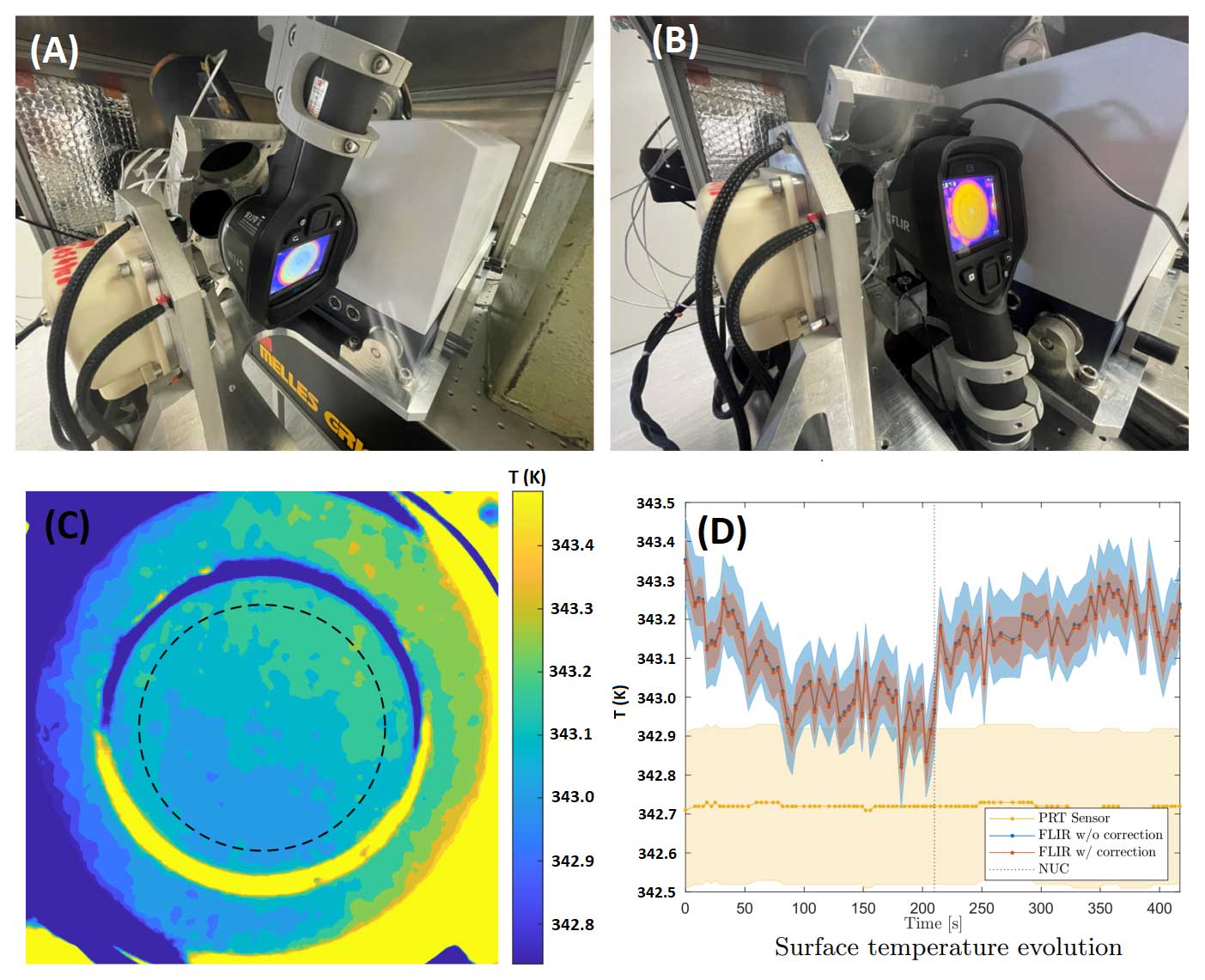
Figure 5 Inverted (a) and upright (b) orientation for the FLIR E8 XT camera measurements used to estimate the spatial uniformity of the hot blackbody. Panel (c) shows the temperature spatial uniformity measured from camera orientation (b) after correction for camera non-uniformity derived from measurements using camera orientation (a). The circle indicated by the dashed line represents the spatial extent of the FINESSE field of view in the plane of the blackbody backplate. (d) Camera mean temperature and root mean square spread for the 100 thermograms obtained over a period of 420 s. PRT values are from the sensor embedded within the hot blackbody backplate 1.5 mm from the emission surface.

Temperature observations for each individual pixel were averaged over the 100 thermograms taken in the inverted orientation when viewing the hot blackbody at 343 K. The average of all pixels within the field of view of FINESSE, defined by the dashed circle in Fig. 5c, was then calculated to obtain a reference “field-of-view-integrated” or “camera mean” temperature. This reference temperature was subtracted from the temporally averaged temperature array to derive a pixel-dependent correction offset. The offset was then applied to the temperature measurements of the blackbody with the camera in the upright orientation. Figure 5c shows a temperature-corrected thermal image of the hot blackbody, with the camera in the upright position. The maximum temperature range within the FINESSE field of view is about 0.3 K. We assess the effectiveness of the correction factor by plotting the camera mean temperature and associated root mean square for each temperature array, with and without correction. These values are plotted in Fig. 5d. The camera mean temperature shows no significant change, but the root mean square has reduced from about 0.1 to 0.05 K.

3.4.3 Blackbody surface emission temperature

Uncertainty in the knowledge of the blackbody surface emission temperature makes the largest contribution to the radiance uncertainty in our calibration. Both the hot and ambient blackbody emission temperatures are derived using the temperature measurement of the PRT100 sensors embedded within the backplate 1.5 mm from the emission surface. In the case of the ambient blackbody, which has no associated heating, the PRT sensor measurement is used as our surface emission temperature, with an uncertainty as defined by the tolerance described in Sect. 3.4.1. For reference, with the hot blackbody at an ambient room temperature of 305.4 K, we see an offset between the mean E8-XT camera temperature and backplate PRT100 temperature measurement of about −0.2 K, the PRT sensor indicating a higher temperature. Figure 5d indicates a +0.5 K offset for the blackbody at 343 K, with the E8-XT camera now indicating a higher temperature. Using similar observations between known blackbody temperatures against an E8-XT camera (Wan et al., 2021), these report E8-XT offsets of +1 and +2 K for target temperatures of 308 and 328 K, respectively, suggesting a rate of change in temperature offset of 0.05 K K⁻¹ over this range. This temperature-dependent offset is also likely to be camera-dependent and means we cannot use the E8-XT camera to directly evaluate the emission temperature of our hot blackbody.

We note that, given the position of the backplate PRT100 between the heaters and emission surface, we expect the PRT100 temperature reading to be higher than the surface emission temperature. Typically, we observe temperature gradients of between +1.2 and +1.6 K between the PRT100s embedded in the front cavity wall and the backplate. The latter always has a higher temperature, and this temperature difference is dependent on the ambient atmospheric conditions. We currently use the mean temperature between the front and rear PRT100 readings for our surface emission temperature. This approach to establishing the surface emission temperature will be further refined in the future: our PRT measurements imply that the current methodology introduces an additional uncertainty of 0.3 K in emission temperature, giving an overall uncertainty of 0.43 K.

3.5 Instrument line shape

The instrument line shape (ILS) is an important parameter required for the simulation, analysis, and interpretation of atmospheric radiative measurements. Previous efforts to determine the ILS of instruments in the EM27 family have indicated that the line shape can be broadened due to self-apodization and can also have notable asymmetry (e.g. Frey et al., 2015; Alberti et al., 2022). Initial inspection of the radiance spectra also suggests that this is the case for FINESSE, so we use the approaches described by Bianchini et al. (2019) and Genest and Tremblay (1999) to model the self-apodization and asymmetric components, respectively.

To assess self-apodization, we concentrate on the impact of the finite solid angle of the radiation propagating through the interferometer broadening the ILS. As described by Bianchini et al. (2019), the impact of the finite solid angle is to broaden and shift spectral lines by convolving the ideal ILS, given by sinc(2πσz_max), by a wavenumber-dependent box function extending from 0 to σ₀Ω/2π in the wavenumber domain. Here, z_max is the maximum optical path, σ₀ is the spectral line centre, and Ω is the finite solid angle.

In the spatial domain, this equates to an additional apodization function which multiplies the boxcar apodization imposed by the finite scan length of ±z_max. What confounds the application of this additional apodization over an extended spectrum is its frequency dependence. This makes deciding on the exact treatment problematic. Bianchini et al. (2019) indicate that if the solid angle contribution to the ILS is small (π/σ₀Ω≫z_max), the apodization can be treated as a linear combination of a boxcar and a triangle function with coefficients α and (1−α), respectively, where α=sinc(z_maxσ₀Ω/2). Using this approach, the self-apodization ILS, ILS(σ)_sa, applied to FINESSE is then determined by the following equation:

$$\begin{array}{}\text{(6)}& \mathrm{\text{ILS}}(\mathit{\sigma }{)}_{\mathrm{sa}}=\mathit{\alpha }\text{sinc}\left(\mathrm{2}\mathit{\pi }\left(\mathrm{\Delta }\mathit{\sigma }\right)\mathit{\sigma }\right)+\left(\mathrm{1}-\mathit{\alpha }\right){\text{sinc}}^{\mathrm{2}}\left(\mathit{\pi }\left(\mathrm{\Delta }\mathit{\sigma }\right)\mathit{\sigma }\right),\end{array}$$

where Δσ is the instrument resolution, which we set to 0.5 cm⁻¹.

To simulate the wavenumber-dependent asymmetric line shape observed in the FINESSE spectra (ILS_asy(σ)), we make use of the geometric description of line asymmetry by Genest and Tremblay (1999) for an off-axis circular detector:

$$\begin{array}{}\text{(7)}& {\text{ILS}}_{\mathrm{asy}}\left(\mathit{\sigma }\right)={\displaystyle \frac{\mathrm{1}}{\mathit{\pi }}}\text{arccos}\left({\displaystyle \frac{r_c^{\mathrm{2}}+f^{\mathrm{2}}\left[{\left(\frac{{\mathit{\sigma }}_{\mathrm{0}}}{\mathit{\sigma }}\right)}^{\mathrm{2}}-\mathrm{1}\right]-R^{\mathrm{2}}}{\mathrm{2}{r}_{c}f{\left[{\left(\frac{{\mathit{\sigma }}_{\mathrm{0}}}{\mathit{\sigma }}\right)}^{\mathrm{2}}-\mathrm{1}\right]}^{\frac{\mathrm{1}}{\mathrm{2}}}}}\right).\end{array}$$

Here, R is the detector element radius, f the detector optical focal length (3.3 cm)m and r_c the detector spatial offset from the optical axis. We define the ILS using a normalized wavenumber scale from 0 to 100 cm⁻¹ on a sampling grid of 0.001 cm⁻¹ and centred on a nominal frequency, σ₀, of 50 cm⁻¹. Although this is not a true representation of the EM27 optical system, which employs a square detector, it does allow us to simulate the observed frequency-dependent asymmetry using Eq. (7) by increasing r_c, the optical axis-to-detector element offset. We reference all dimensions relative to f. With R set to 0.005f, which suggests the source is underfilling the detector, we find that varying r_c between 0.005f and 0.012f over the spectral range from 400 to 1600 cm⁻¹ gives a reasonable fit to the observed asymmetry. This manifests in the spectra as a slight shift in the line centre towards lower wavenumbers and a low wavenumber foot evident at the base of the line, as one might expect from the asymmetry components shown in Fig. 9a. The wavenumber-dependent shift in r_c indicates that there may be some optical induced dispersion of the beam, possibly in the beam splitter or the window of the detector housing.

We determine the ILS for FINESSE using water-vapour absorption lines in the regions of 400–500 and 1300–1600 cm⁻¹. Specifically, we compare the measured to simulated transmittance of the air path between the FINESSE diamond window and blackbodies. Measured transmittances are derived from the set of external calibration measurements described earlier and shown in Fig. 3, which are compared to equivalent measurements of the internal calibration target, obtained under similar instrument environmental conditions. The average instrument spectral responses for both of these sets of measurements are shown in Fig. 6a. The spectral response derived from the internal target is considerably higher than that derived from the external targets due to reflection and transmission losses of the diamond window. We ratio the two responses, allowing for these losses, to obtain an “apparent” transmission spectrum for the path between the diamond window and external blackbodies (Fig. 6b). The relative humidity within the spectrometer was approximately 2 % for both sets of measurements, and the associated absorption is assumed to be cancelled out in the ratio.

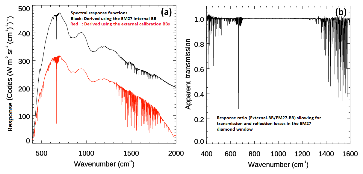
Figure 6 (a) The instrument spectral responses derived using the internal blackbody (black) and external FINESSE calibration targets (red). (b) “Apparent” external air path transmission between the FINESSE calibration targets and EM27 input window derived by taking the ratio of the spectral response curves, allowing for the transmission losses in the diamond window transmission (0.675) and an estimate of absorption due to the diamond phonon absorption (Bennett et al., 2014) towards 1600 cm⁻¹.

Simulated transmittances are obtained from radiative transfer modelling using the average humidity, temperature, and pressure observed over the measurement period (Fig. 3c and d) as input to LBLRTM V12.13 (Clough et al., 2005). These “ideal” values then need to be modified by the FINESSE ILS: this modification is performed iteratively for different values of ILS_sa and ILS_asy, with the optimal ILS chosen to be that which minimizes the residual between the measured and simulated transmittances in the vicinity of spectral absorption features.

To deduce the optimal ILS, we consider 13 frequency bins of varying widths, starting from 400 cm⁻¹ and extending to 1600 cm⁻¹. For increasing wavenumber (increasing bin number), a series of asymmetric ILS components are calculated using Eq. (7) by increasing the initial r_c offset chosen for the 400 cm⁻¹ bin in equal steps up to the 1600 cm⁻¹ bin. This is equivalent to a frequency-dependent misalignment between the detector and optical axis, which, if it is the cause of the asymmetry, suggests an optical component is causing dispersion. This results in an asymmetry which increases with the increase in wavenumber. A set of asymmetry arrays, consisting of an asymmetric component, can then be calculated for each wavenumber bin by modifying the initial r_c offset and rate of change in r_c.

Separately to this, we generate an equivalent set of arrays which consist of the self-apodization ILS components for each wavenumber bin. Each array is obtained by fixing the solid angle, calculating the equivalent alpha terms, and generating ILS(s)_sa according to Eq. (6). A set of these self-broadened ILS arrays is generated by adjusting the solid angle between arrays.

The asymmetric and self-apodized ILS arrays are then convolved for each wavenumber bin and applied to the simulated transmission. When optimizing the ILS convolved simulation with the observations, we also need to adjust the observations for slight optical alignment offsets between the metrology sampling laser and the mid-infrared optical axis. An optical misalignment results in a scaling of the sampling interval, which, to first order, is constant in dσ/σ, where dσ is the wavenumber offset at a given wavenumber. We find that a frequency scaling of 1.00016 adequately corrects the FINESSE observations. The entire ILS determination process is summarized in Fig. 7.

Figure 7 Flowchart showing the retrieval method for the FINESSE ILS.

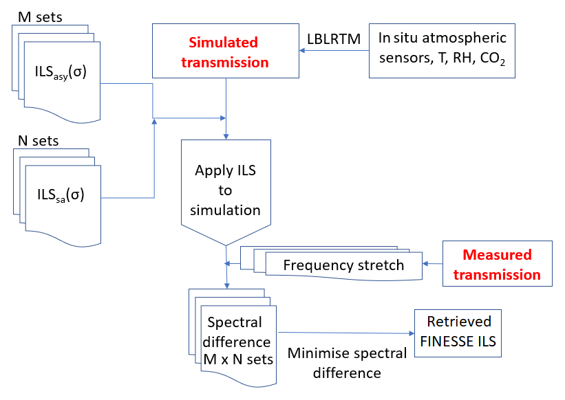
Figure 8a shows the apparent transmission plotted over by the simulated transmission after the optimal ILS has been applied. Differences, in blue, are less than 1 % below 500 cm⁻¹ and on the order of 2 % towards 1600 cm⁻¹. Panels (b) and (c) highlight regions of strong water-vapour absorption where the largest residuals are seen. Figure 9a and b show the ILS_asy (Eq. 7) and alpha values (Eq. 6) that lead to the optimal ILS. This optimal ILS (Fig. 9c) clearly has a strong frequency-dependent asymmetry and a self-apodization component, which also depends on the wavenumber.

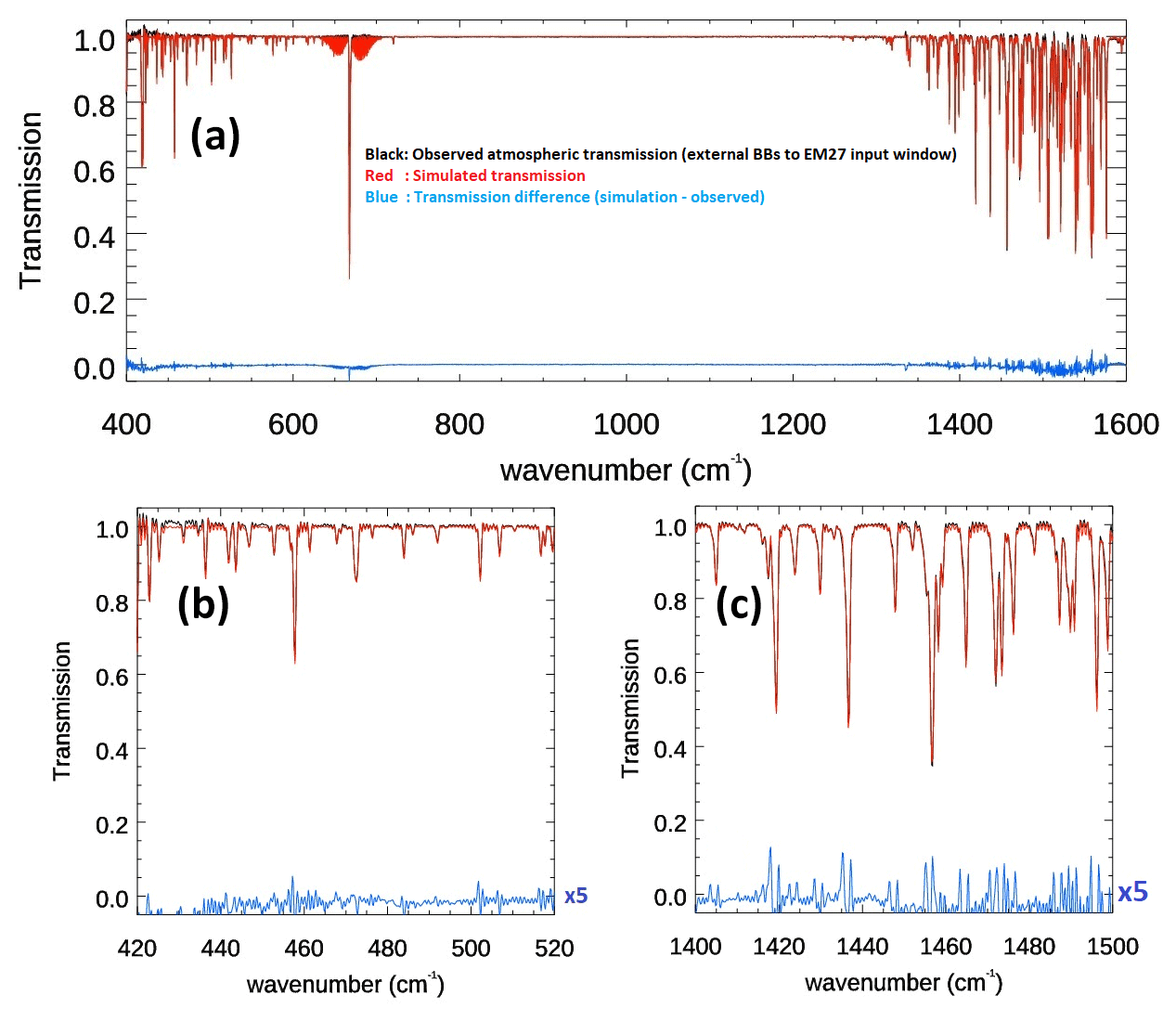
Figure 8 (a) Observed atmospheric transmission (black), simulated transmission (red), and residual between the two (blue) for the optimal FINESSE ILS. Panels (b) and (c) highlight the two water-vapour absorption regions used to minimize the residuals. The residuals have been scaled by a factor of 5 to allow for them to be distinguished.

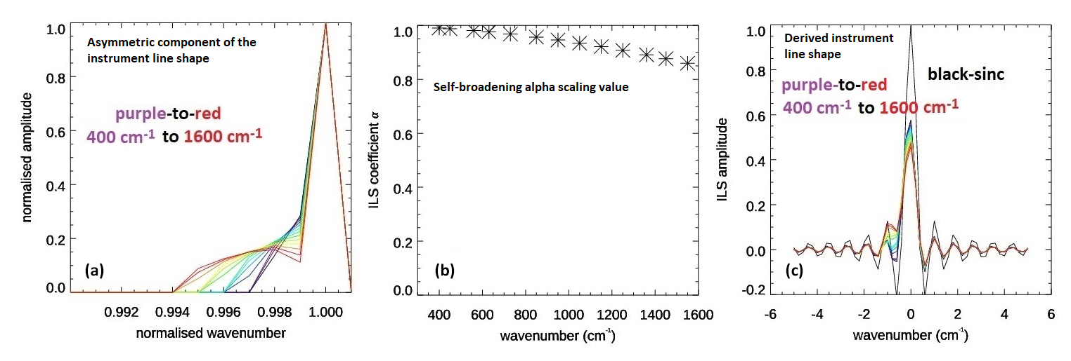
Figure 9 (a) The asymmetric component of the ILS defined by Eq. (7), plotted as an ILS for increasing frequency. (b) The FINESSE alpha scaling value used in Eq. (6) that best represents the observed ILS self-apodization and is equivalent to a solid angle of 0.001 sr. (c) The best-fit ILS, derived from a combination of asymmetry and self-broadening terms.

4 Calibration and radiance uncertainties: application to clear-sky observations

To illustrate FINESSE performance, we highlight zenith-view observations made from Imperial College London on 23 March 2022 from 09:00–13:00 UTC. Examples of calibrated radiances, L(σ)_scene, are shown in Fig. 10. These radiances are derived using Eq. (8), where the variables are as defined in Eq. (4) and I(x)_scene is the acquired interferogram for the given scene.

$$\begin{array}{}\text{(8)}& \begin{array}{rl}& L(\mathit{\sigma }{)}_{\mathrm{scene}}\\ & =\left[{\mathit{\epsilon }}_{\mathrm{eff}}\left(\mathit{\sigma }\right)B{\left(\mathit{\sigma },T\right)}_{\mathrm{hot}}+\left(\mathrm{1}-{\mathit{\epsilon }}_{\mathrm{eff}}\left(\mathit{\sigma }\right)\right)L(\mathit{\sigma }{)}_{\mathrm{hot}}^{\mathrm{ext}}\right]\\ & -{\displaystyle \frac{\text{FFT}\left\{I(x{)}_{\mathrm{hot}}-I(x{)}_{\mathrm{scene}}\right\}}{R(\mathit{\sigma }{)}_{\mathrm{FIN}}}}\end{array}\end{array}$$

R(σ)_FIN is derived from calibration observations taken before and after the scene views and $L(\mathit{\sigma }{)}_{\mathrm{hot}}^{\mathrm{ext}}$ is given by the Planck function using the temperature from a surface mounted PRT100 sensor on the EM27 enclosure. Typically, we set the observation cycle to undertake 1 min of measurements of the hot BB followed by 1 min of ambient blackbody views. Dependent on the instrument stability and requirements for the experiment, we can vary the scene-view measurement period from 1 to 4 min. During this scene-view period, we may repeat a given view angle or vary the view angle to undertake surface and sky-view measurements; regardless, these data are acquired in sets of 1 min periods.

When deriving the uncertainties in the FINESSE-calibrated radiances, we differentiate between spectrally correlated and uncorrelated components. This is important as spectrally uncorrelated detector noise, which we refer to as noise-equivalent spectral radiance (NESR), can be reduced through spectral or temporal averaging, whereas, for instance, the uncertainty in the calibrated radiances, due to knowledge of the absolute temperature of the PRT100 sensors, is fixed for a given observational setup and will yield a spectrally correlated shift in the calibrated radiance, which cannot be reduced through averaging.

It should be noted that if the temperature of the hot calibration target, T_hot, which appears in the first term on the right-hand side of Eq. (8), is greater than the “true” emission temperature, ΔT_hot > 0, then this term will introduce a positive radiance offset. However, the response function, R(σ)_FIN, also uses T_hot and decreases for ΔT_hot > 0 (Eq. 4). The last term in Eq. (8) will therefore also increase with increasing ΔT_hot and acts to help compensate for the first term. Similarly, any offset in the effective emissivity relative to the “true” emissivity will see some compensation between the first and third terms of Eq. (8). Uncertainty in the ambient blackbody temperature, T_amb, only impacts the spectral response function, so, for this variable, there are no compensating terms. However, as this ambient blackbody has high thermal mass and no heating sources, we expect no significant thermal gradients between the PRT100 and emission surface. We therefore combine the uncertainty associated with the PRT100 itself with knowledge of the small thermal drift observed during the calibration scans to estimate the uncertainty in T_amb.

Any observed external radiance seen in the reflection from the hot blackbody, which is included as the second term on the right-hand side of Eq. (8), can be mitigated for by increasing the effective emissivity of the calibration target as discussed in Sect. 3.3.

4.1 Evaluating radiance uncertainties

4.1.1 Detector noise (NESR)

The calibrated radiances shown in Fig. 10a are for a set of 80 sequential scans. The raw spectra were calibrated using the mean spectral response function of the calibration scans before and after the zenith view. The hot blackbody observations used in Eq. (8) were also an average of the hot blackbody measurements from before and after these zenith-view measurements. Assuming negligible change between successive scans, we estimate the NESR for a single scan from the set of 79 differences between the 80 successive calibrated scans; these differences are shown in Fig. 10b.

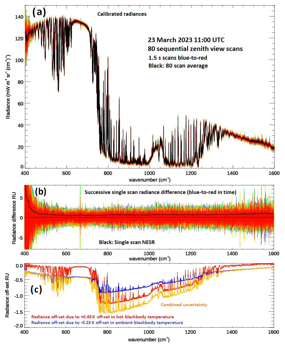
Figure 10 (a) Individual calibrated radiances obtained over a 2 min view period colour-coded from blue to red in time. Plotted over in black is the average of these scans. (b) Radiance differences between successive scans with NESR for a single scan plotted over in black. (c) Calibrated radiance offset introduced when applying a +0.43 K offset to the hot blackbody temperature (red) or a −0.23 K offset to the ambient blackbody temperature relative to their estimated emission temperatures (1 RU = 1 mW m⁻² sr⁻¹ (cm⁻¹)⁻¹).

For each of these 79 difference spectra shown in Fig. 10b, blue to red, we calculate the spectrally resolved NESR from the root mean square value derived from a rolling bin that is 5 cm⁻¹ in width centred on sequential wavenumbers covering the full spectral range. To improve the overall assessment of these NESR estimates, we take the average of the 79 NESR estimates. As the calibration scans are averages of 80 hot and ambient target measurements, the dominant noise on the calibrated radiance difference will be a combination of the two successive zenith measurements. Assuming the detector noise is incoherent, we divide the spectrally resolved NESR described above by the square root of 2 to give the resultant single-scan NESR, this is shown in Fig. 10b as the overlying black line.

4.1.2 Correlated uncertainty

We have discussed the impact of offsets between the estimated emission temperature and the true surface emission temperature. Along with the PRT100 accuracy of 0.2 and 0.29 K for the ambient and hot targets (Sect. 3.4.1), there is a temperature drift over the 1 min observation period for each target view seen in both our laboratory and outdoor measurements. For the ambient target, we observe an upwards drift of about 0.1 K min⁻¹ indoors, while the hot target temperature is controlled to within 0.1 K over the same period, as shown in Fig. 4b. Outdoors, the drift in the ambient blackbody temperature generally follows the ambient air temperature but we have seen variations associated with changes in wind direction or gustiness. For the outdoor measurements shown here, the ambient blackbody temperature variation was similar to the 0.1 K min⁻¹ seen in the laboratory. Our measurements in Sect. 3.4.2 indicate a spatial variation of 0.05 K across the blackbody target apertures. In addition, for the hot blackbody, following the discussion in Sect. 3.4.3, we factor in an additional 0.3 K uncertainty due to along-axis thermal gradients. Combining all of these uncertainties results in final uncertainties of 0.23 and 0.43 K for the ambient and hot blackbody emission temperature, respectively.

Figure 10c shows the impact on the calibrated radiance if a recalibration is performed using blackbody emission temperature offsets of +0.43 K for the hot and −0.23 K for the ambient blackbodies. Over wavenumber ranges sampling warmer atmospheric levels (400 < s < 700 cm⁻¹ and 1250 < s < 1600 cm⁻¹), the calibrated radiance is more sensitive to offsets in the ambient blackbody temperature than to offsets in the hot blackbody temperature. This lower sensitivity to offsets in the hot target is due to the self-compensation effects discussed earlier in Sect. 4. At wavenumbers sounding a colder scene temperature (700 < s < 1250 cm⁻¹), the effectiveness of this compensation reduces and the calibrated radiance becomes more sensitive to offsets in the hot blackbody than those associated with the ambient blackbody.

4.2 Observation–simulation comparison

We have not yet had the opportunity to undertake a full radiative closure study using FINESSE and co-located atmospheric soundings, so, for the purpose of demonstrating performance, we undertake a comparison of the observed zenith-view spectra against a simulation from LBLRTM using profiles taken from ERA5 37-level 0.25° × 0.25° gridded array (Hersbach et al., 2020). Figure 11 shows the temperature and humidity profile from 11:00 UTC on 23 March 2022 as recorded by ERA5 at the grid point that is nearest to the observations. The balcony from which the observations were made is at an altitude of 30 m above sea level. The ambient pressure, temperature, humidity, and CO₂ concentrations obtained from the Vaisala sensors described in Sect. 2.3 were used to set conditions at the surface, with the ERA5 pressure, temperature, humidity and ozone values superposed above. Above the surface, CO₂ concentrations were set at 420 ppmv.

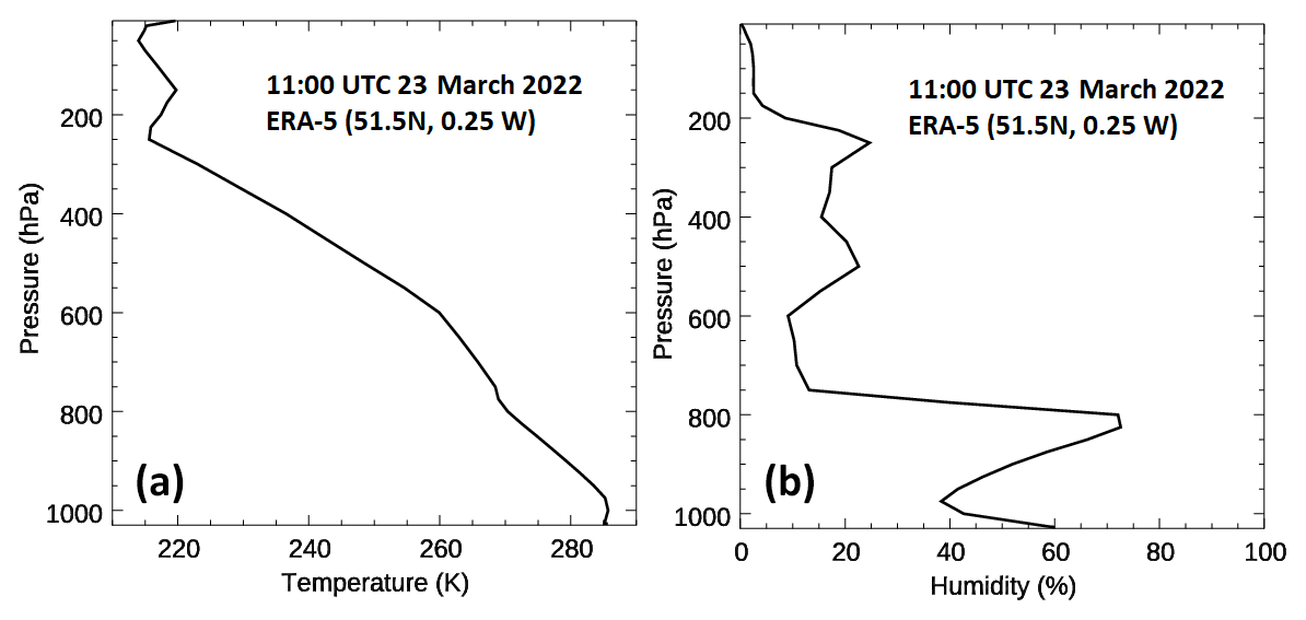
Figure 11 ERA5 profiles of (a) temperature and (b) relative humidity from 11:00 UTC on 23 March 2022 for the grid box that is closest to the FINESSE measurements.

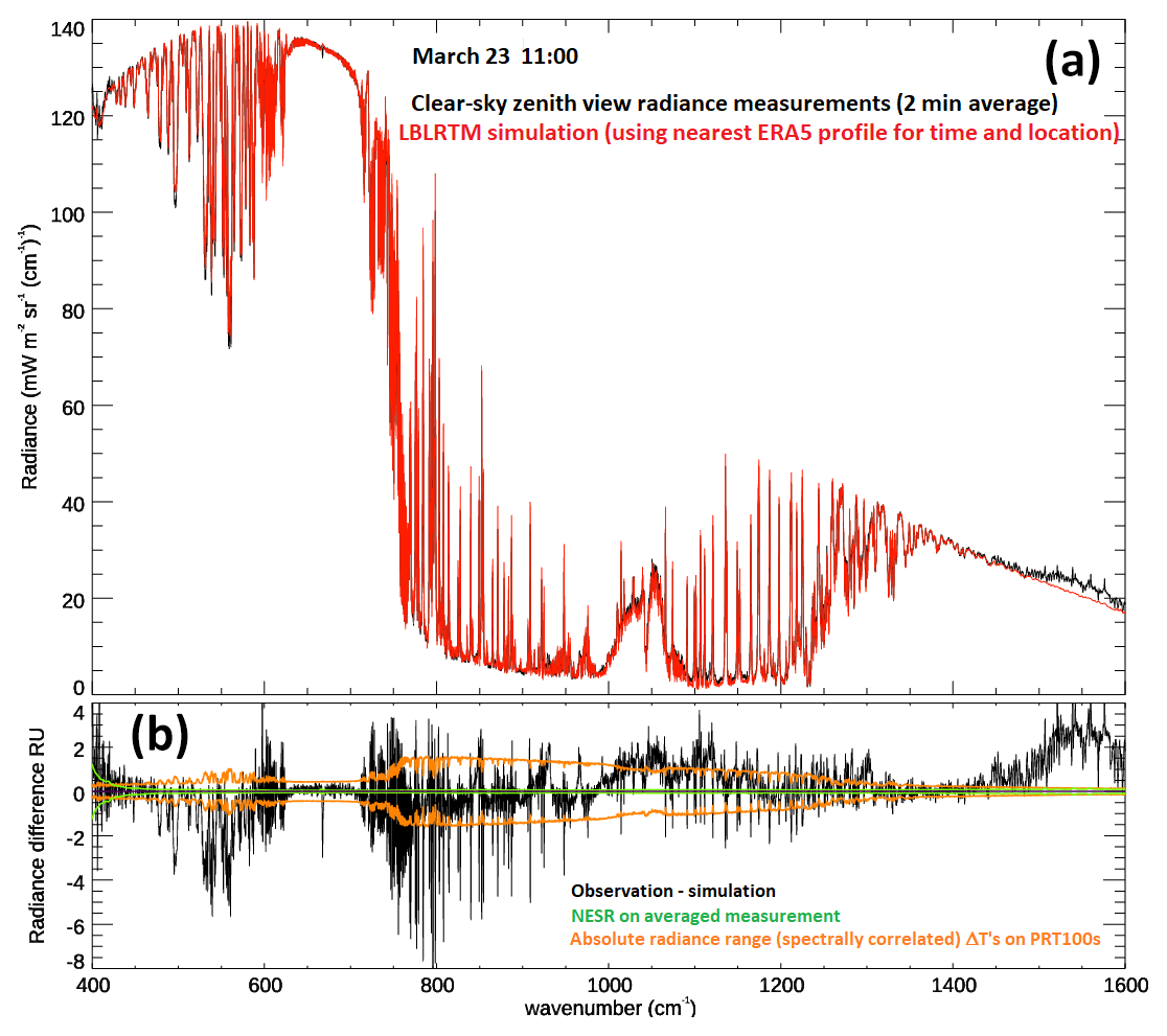
Figure 12 (a) Calibrated radiance spectrum, derived from 2 min of observations, for the zenith scan cycle around 11:00 UTC, with corresponding LBLRTM simulation. (b) Radiance difference between measurement and simulation. The radiance offsets associated with the uncertainty in blackbody surface emission temperature and the NESR for the 2 min average spectrum are also shown.

Figure 12a shows the 2 min averaged observed spectrum closest to 11:00 UTC, with the corresponding apodized LBLRTM simulation plotted over. Figure 12b shows the difference between observation and simulation with the NESR and calibration radiance offset envelope associated with uncertainty in the blackbody surface emission temperature plotted over for comparison. We expect strongly absorbing spectral regions to give good agreement with the simulation as the near-surface temperature, humidity, CO₂, and pressure is strongly influenced by the Vaisala measurements and, indeed, we see good agreement between the simulations and observations within the centre of the 15 µm CO₂ band (620–710 cm⁻¹) and within the band wings of the 6.3 µm water-vapour vibration–rotation band (1350–1450 cm⁻¹). Agreement is also very good within the atmospheric window (800–1250 cm⁻¹) outside of the 9.6 µm ozone band and isolated line features. This general agreement is very encouraging given the fact that the ERA5 profile is representative of a much larger spatial scale than the narrow vertical profile from FINESSE, with radiance differences generally falling within the range of the measured radiance uncertainty. The obvious exception occurs at wavenumbers above 1450 cm⁻¹, where we see an increase in observed radiance. We believe that this is likely due to uncorrected emission/absorption from the diamond phonon band occurring within the EM27 entrance window.

To probe the comparison in more detail, Fig. 13 shows the simulation and observation across expanded frequency ranges along with the radiance differences. Panels (a) and (c) suggest that the ERA5 profile is too wet, with simulated radiances in far-infrared micro-windows appearing to be slightly too opaque relative to the measurements. Over these wavenumbers, we see no significant evidence of line-wing-dependent residuals, implying that the estimated FINESSE ILS is a good fit. For the spectral range of 900–1000 cm⁻¹ (panels b and d), we see some evidence at 910 cm⁻¹ (and 920 and 948 cm⁻¹) of an asymmetric difference around zero that is likely due to the veracity of our estimate of the ILS. Interestingly, the broader spectroscopic features at 930 and 965 cm⁻¹ look real and are likely due to NH₃, whose absorption was not included in the LBLRTM simulation. From 1200 to 1250 cm⁻¹ (panels e and g), we do see residuals around zero that suggest the retrieved ILS may not be sufficiently modelling the true line profile; this is in keeping with the residuals seen in Fig. 8b and c. Over the range of 1280 to 1320 cm⁻¹ and outside of CH₄ absorption centred at around 1300 cm⁻¹, which is not included in our simulation, panels (f) and (h) show that the differences fall within the uncertainties.

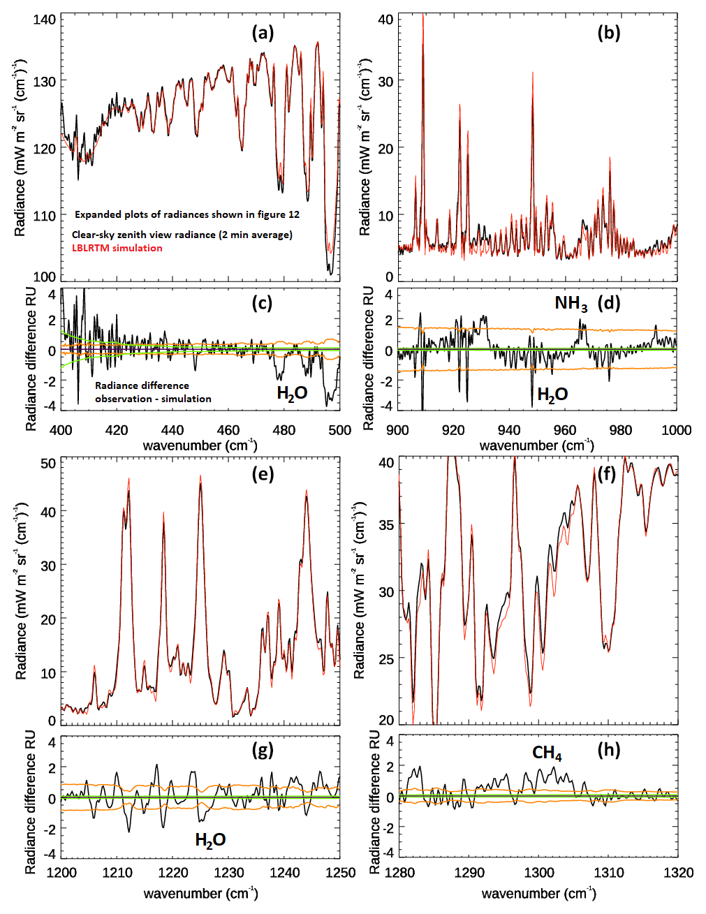
Figure 13 Expanded views of the radiance observation and simulation (a, c, e, g) and associated differences (b, d, f, h) shown in Fig. 12 for selected wavenumber ranges with identical colour-coding.

5 Discussion and conclusions

This paper has provided an outline of the Far-INfrarEd Spectrometer for Surface Emissivity (FINESSE), which combines a commercial Bruker EM27 spectrometer with a front-end calibration and scene-selection rig designed at Imperial College London in order to facilitate emissivity retrievals extending into the far-infrared. We have discussed the two-point calibration procedure and shown that the instrument spectral response is stable to within ±0.2 % over several hours over the majority of its spectral range (400–1600 cm⁻¹).

An important aspect of any new instrumental development is the characterization of uncertainty. We have taken great care to provide realistic assessments of the contribution of different error sources, particularly focusing on our knowledge of the blackbody targets effective emissivity and emission temperature. Using these estimates, we have established an initial overall budget for the blackbody emission uncertainty, providing a baseline for FINESSE's calibration uncertainties. Additionally, we have used laboratory measurements to establish an initial estimate of the spectrally varying ILS, which is a requirement for future emissivity and atmospheric profile retrieval efforts. Together with previous work which investigated non-ideal instrument line shapes within their EM27/SUN spectrometers (Frey et al., 2015, 2019), our estimate shows that the FINESSE ILS is highly asymmetric and that this asymmetry is frequency-dependent.

Clear-sky zenith measurements from FINESSE have been used to derive the radiance sensitivity in the form of a single-scan NESR. Comparison to radiative transfer simulations driven by temporally and spatially coincident ERA5 profiles shows encouraging agreement given the limitations of the ERA5 spatial scale relative to the much narrower spatial view of FINESSE. By removing specific gaseous species, the simulations also hint at the sensitivity that the instrument will have to specific absorbers such as NH₃ and CH₄.

One feature that does need further investigation is the anomalous emission between 1450 and 1600 cm⁻¹, which we attribute to unaccounted for emission from the instrument diamond window (Shi et al., 2021). Although this currently precludes the use of the FINESSE observations in this part of the spectrum, it is not an issue for emissivity retrievals, which primarily use measurements from the main atmospheric window and the so-called dirty window in the far-infrared. Part 2 (Warwick et al., 2024) of this paper validates the operational capability of FINESSE by undertaking emissivity retrievals of de-ionized water in the spectral range 400–1400 cm⁻¹. The emissivity of de-ionized water has been well studied in the mid-infrared and offers the opportunity for cross-comparison/validation of the FINESSE-retrieved emissivities with literature values as well as extending emissivity measurements into the far-infrared.

Finally, we note that, despite its name, FINESSE is not limited to emissivity retrievals. Recently, the instrument was deployed to Andøya, Norway, to undertake measurements in support of the FORUM mission. The observations obtained during the campaign encompass both clear-sky and cloudy-sky zenith radiances as well as down-looking views of snow and ice. These radiances have been calibrated using the approach outlined in this paper and are currently being evaluated both at Imperial, ESA, and by colleagues at CNR Italy. We anticipate that these collaborative studies will help refine our knowledge of the uncertainty budget and ILS estimates described here, enhancing the utility of FINESSE for future deployments.