the Creative Commons Attribution 4.0 License.
the Creative Commons Attribution 4.0 License.
 | 27 Aug 2024
High-resolution wind speed measurements with quadcopter uncrewed aerial systems: calibration and verification in a wind tunnel with an active grid
Johannes Kistner
Lars Neuhaus
Norman Wildmann
As a contribution to closing observational gaps in the atmospheric boundary layer (ABL), the Simultaneous Wind measurement with Uncrewed Flight Systems in 3D (SWUF-3D) fleet of uncrewed aerial systems (UASs) is utilized for in situ measurements of turbulence. To date, the coefficients for the transformation terms used in our algorithm for deriving wind speeds from avionic data have only been determined via calibration flights in the free field. Therefore, we present in this work calibration and verification under laboratory conditions. The UAS measurements are performed in a wind tunnel equipped with an active grid and constant temperature anemometers (CTAs) as a reference. Calibration is performed in x- and y-coordinate directions of the UAS body frame at wind speeds of 2 … 18 m s−1. For systematic verification of the measurement capabilities and identification of limitations, different measurement scenarios like gusts, velocity steps, and turbulence are generated with the active grid. Furthermore, the measurement accuracy under different angles of sideslip (AoSs) and wind speeds is investigated, and we examined whether the calibration coefficients can be ported to other UASs in the fleet. Our analyses show that the uncertainty in measuring the wind speed depends on the wind speed magnitude and increases with extreme velocity changes and with higher wind speeds, resulting in a root-mean-square error (RMSE) of less than 0.2 m s−1 for steady wind speeds. Applying the calibration coefficients from one UAS to others within the fleet results in comparable accuracies. Flights in gusts of different strengths yield an RMSE of up to 0.6 m s−1. The maximal RMSE occurs in the most extreme velocity steps (i.e., a lower speed of 5 m s−1 and an amplitude of 10 m s−1) and exceeds 1.3 m s−1. For variances below approx. 0.5 and 0.3 m2 s−2, the maximal resolvable frequencies of the turbulence are about 2 and 1 Hz, respectively. The results indicate successful calibration but with susceptibility to high AoSs in high wind speeds, no necessity for wind tunnel calibration for individual UASs, and the need for further research regarding turbulence analysis.
- Article
(3215 KB) - Full-text XML
- BibTeX
- EndNote


Uncrewed aerial systems (UASs) are steadily gaining popularity for measuring the wind in the atmospheric boundary layer (ABL). There are several approaches to measuring the wind vector (i.e., wind speed and direction), which can be grouped into two main categories: first, direct wind measurement, in which a UAS used as a sensor platform carries an anemometer (e.g., ultrasonic anemometer, multi-hole probe, lidar, or hot-wire anemometer) as a payload. Here, the UAS can be a fixed-wing aircraft (Wildmann et al., 2015; Platis et al., 2018; Rautenberg et al., 2019; zum Berge et al., 2021) or a multicopter (Palomaki et al., 2017; Shimura et al., 2018; Nolan et al., 2018; Molter and Cheng, 2020). The second approach is indirect wind measurement, in which the avionic data of a UAS (e.g., Euler angles, accelerations, and motor thrust) are used to derive the wind that a multicopter UAS is exposed to while hovering (Palomaki et al., 2017; Simma et al., 2020; Shelekhov et al., 2022) or while in steady directional flight (Brosy et al., 2017; Segales et al., 2020; Hattenberger et al., 2022; González-Rocha et al., 2023). For this measurement method, knowledge of particular aerodynamic or flight dynamic characteristics of the respective UAS is necessary, which is usually not given a priori. This is why calibration of the wind measurement with the respective UAS model becomes necessary.
The wind estimation with the SWUF-3D (Simultaneous Wind measurement with Uncrewed Flight Systems in 3D) fleet (Wetz et al., 2021; Wildmann and Wetz, 2022) for determination of turbulence in the ABL (Wetz and Wildmann, 2023; Wetz et al., 2023) is also based on the latter technique. Using this method, turbulence with length scales from 5 m can be resolved. The previously used calibration coefficients of the fleet and their validations have been performed in open-field measurements up to this point (Wetz and Wildmann, 2022), which always have inherent uncertainties. This motivates the first part of this work: the calibration of the coefficients of the extended Rayleigh drag equations of the wind measurement algorithm from Wetz and Wildmann (2022) under controlled laboratory conditions. The calibration is carried out for mean wind speeds along the main axes (x and y direction) of the fixed-body coordinate system of a single UAS.
Calibration for the fleet based on only one UAS comes from the idea that by porting the determined calibration coefficients to other UASs of the same type but with potential production variations (e.g., autopilot orientation), those other UASs are also capable of accurately measuring the wind. Furthermore, this approach is subject to the hypothesis that calibration along the longitudinal and lateral axes of the UAS will allow reliable wind measurement at angles of sideslip (AoSs) off those axes, i.e., applicability in the case of divergent inflow conditions. More generally, the overall approach is based on the hypothesis that it is possible to reliably measure highly dynamic flows with the UAS via calibration in averaged wind speeds. For this purpose, we perform verification in reproducible flow scenarios designed to cover real-world applications, along with a systematic determination of the limitations of the turbulence measurement.
Wind tunnel measurements for comparable purposes have already been carried out before by a series of different studies: Hattenberger et al. (2022) performed their measurements not in a wind tunnel but indoors with a wind generator. Wang et al. (2018) also verified their wind measurement in an indoor experiment but at very low, constant velocities (< 2 m s−1). Thielicke et al. (2021) performed wind tunnel calibration and testing of their system as well, which, however, features an ultrasonic anemometer attached to a multicopter and thus counts as a direct wind measurement technique. González-Rocha et al. (2019) conducted wind tunnel tests as part of their review of various indirect measurement techniques but only for the rotor and not the entire UAS. Marino et al. (2015) carried out wind tunnel calibrations for their measurement method using the power consumption of the rotors, but they conclude its practicality to be limited. The most closely related work to our study is the research of Neumann and Bartholmai (2015). They determined the drag coefficient of their UAS in the wind tunnel at sideslip angles of 0, 45, and 90° to the main wind direction with wind speeds up to 8 m s−1 in order to enable determination of the wind speed via the Rayleigh drag equations and the system described by Neumann et al. (2012).
Going beyond that, the work presented in this paper aims to determine the additional calibration coefficients of the extended Rayleigh drag equation of the wind measurement algorithm from Wetz and Wildmann (2022) for a significantly extended velocity envelope. Other aims of this work are the systematic investigation in the wind tunnel of the coefficients' applicability in more complex flow conditions, applicability in the case of several divergent inflow conditions off the main axes, and applicability to the entire fleet. These analyses distinguish our work from the state of research. We highlight that this is the first time that wind measurements have been performed with a multicopter UAS in the reproducible turbulent flow fields of a wind tunnel with an active grid. The underlying hypotheses mentioned above lead to the following research questions.
-
What are the wind measurement accuracies at different angles of sideslip?
-
What are the measurement accuracies for different UASs using the same calibration coefficients?
-
What are the accuracies in more complex flow conditions in terms of wind speed, response time behavior, and resolution?
Thus, this study aims to gain enhanced data for calibration along with the systematic detection of measurement limitations or potential situations in which the wind measurement method is subject to higher uncertainties. It is not intended to replace validation in the open field or to give conclusions about measurement capabilities when measuring with the entire fleet. In the next section, a description of our UAS and the wind measurement system, as well as the wind tunnel including the reference sensors, are given. In Sect. 3, the procedures for calibration and verification are explained. The results are presented in Sect. 4 and discussed in Sects. 5 and 6.
Our experimental setup consists of a UAS, which we measure against reference sensors in a wind tunnel with an active grid. These systems are described in more detail below. The full setup used is shown in Fig. 1.
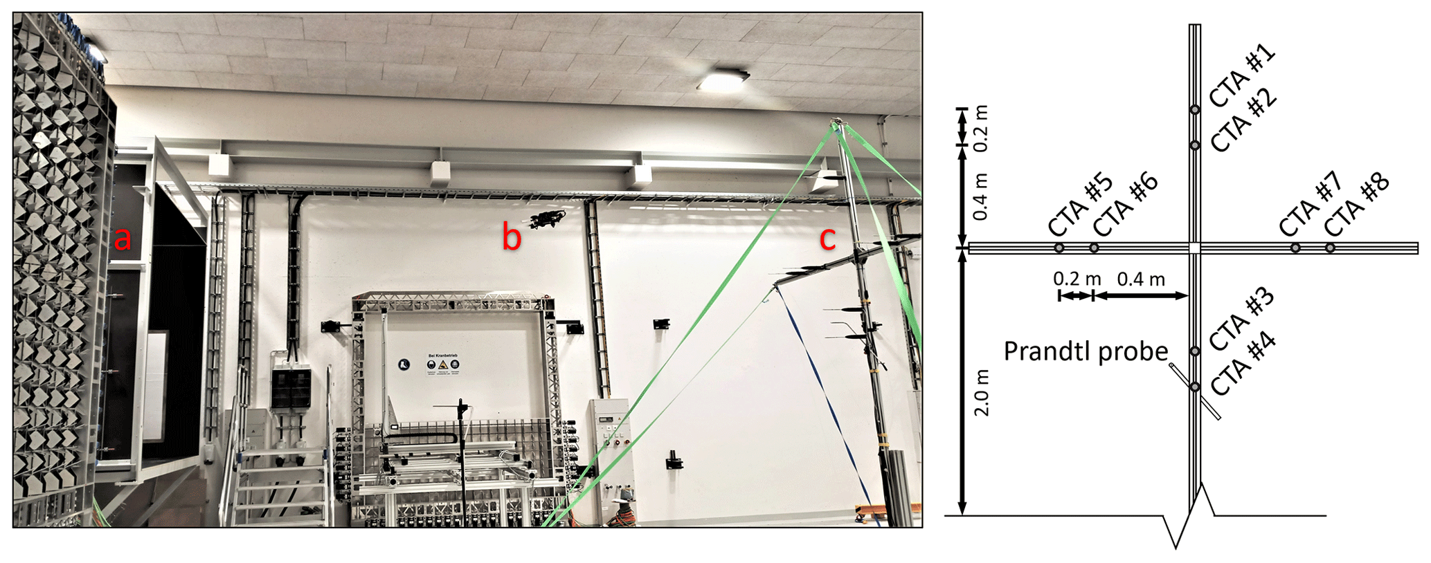
Figure 1Left: measurement setup in the wind tunnel with (a) an active grid at the outlet, (b) a UAS at approx. 2.5 m downstream, and (c) the reference sensor cross at 5 m downstream. Right: schematic front view of the reference sensor cross with positions of the CTAs and Prandtl probe.
2.1 UAS and wind measurement
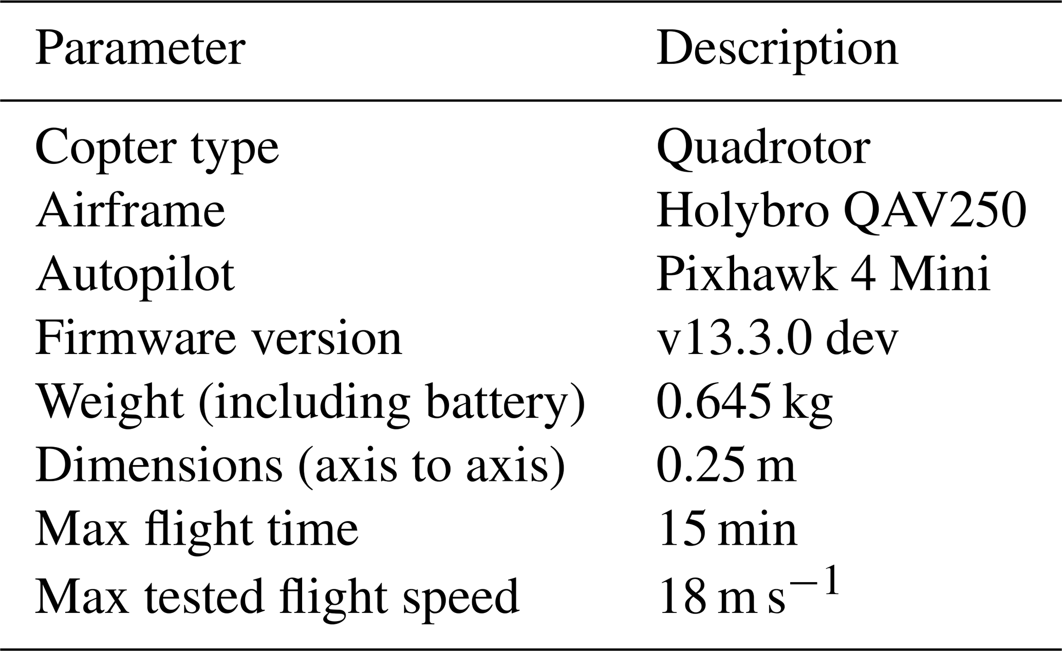
The type of UAS used in this work is a quadcopter. It is based on the Holybro QAV250 airframe and the Pixhawk autopilot, running a custom version of the PX4 firmware (Table 1). The copter measures 0.25 m in the diagonal from rotor to rotor and weighs 0.645 kg, including battery. A flight duration of up to 15 min can be achieved, depending on wind conditions. For a more detailed description of the hardware, refer to Wetz et al. (2021) and Wetz and Wildmann (2022).
Wind measurements are taken by hovering the UAS in one place and always turning its nose automatically into the wind by applying PX4's weather vane mode. During this operation, the attitude of the UAS is tracked by measuring and logging the avionic data with a temporal resolution of 1 to 250 Hz, depending on the particular sensor. The wind acting on the UAS during hover can be determined by applying the wind algorithm using the modified Rayleigh drag equation in Eq. (1) (see Wetz et al., 2021; Wetz and Wildmann, 2022 for a more detailed description) to the measured attitude and its first and second derivatives. More precisely, the wind vector,
consisting of the longitudinal wind speed component u and the lateral component v in the geodetic coordinate system, is calculated from the wind forces Fw,i determined from the avionic sensors and the calibration coefficients ci and bi. Since the forces and coefficients are given in the body-fixed coordinate system, they have to be converted into the geodetic coordinate system using the rotation matrix R based on the Euler angles pitch θ, roll ϕ, and yaw ψ (Eq. 2). Motions of the UAS that deviate from a stationary hover are detected by the GNSS (, ) and corrected in the calculation, using GNSS data fused with other sensor information given by the autopilot. This means that wind speed and wind direction can be measured without an additional wind sensor.
The sensors used include accelerometers, gyroscopes, magnetometers, barometers, and GNSS receivers in the free field. Since sufficient GNSS signal reception is not available in the wind tunnel, an optical positioning system is used there instead. This consists of the Hex HereFlow optical flow sensor for holding the position in longitudinal and lateral earth coordinate directions and the Benewake TF-Mini rangefinder for holding the altitude over the ground. These sensors are very small and lightweight, so their effects on drag and weight are negligible. The rangefinder performs sufficiently well. However, the optical flow sensor type used has an inherent imprecision, which causes the UAS to drift away while hovering. In calm air, the positional drift is about 1 m min−1. As wind speeds increase, the intensity and direction of the drift change without an identifiable pattern, which required constant adjustment to counteract the drift during the test flights. These adjustments were executed by the remote pilot through manual trim. Dedicated flight tests have shown the comparability of the wind measurement using the positioning via optical flow and trim versus the positioning via GNSS.
2.2 Wind tunnel
The measurements are performed in the turbulent wind tunnel in Oldenburg (Kröger et al., 2018). The wind tunnel has a test section that measures 3 × 3 m2 with a length of 30 m. In the open configuration, wind speeds up to 32 m s−1 can be achieved by 4 fans of 110 kW each. The centerpiece of the turbulent wind tunnel is the active grid, which is attached to the nozzle. The active grid covers the entire area of 3 × 3 m2 and consists of 80 individual controlled shafts with a mesh width of 0.143 m. The active grid allows one to change its blockage dynamically and locally from 21 % to 92 %. To tailor turbulent flows and generate specific flow structures, the blockage-induced flow design approach is used (Neuhaus et al., 2021). Based on a transfer function between shaft angle and wind speed, specific shaft angle time series can be determined for individual shaft motion groups. In this way, the approach allows for very strong velocity variations on short timescales over a large cross-sectional region. The shaft motion groups chosen in this work produce approximately homogeneous flow characteristics over an area of 2 × 2 m2. Within this area and the main measurement zone of the UAS, with the active grid completely open and inoperative, we determined a standard deviation of 0.06 and 0.14 m s−1 for 1 min averages of wind speeds at 5 and 10 m s−1, respectively, whereby the deviation in the lateral direction is higher towards the grid. To excite the largest scales, an additional dynamic excitation is done using the wind tunnel fans (Neuhaus et al., 2020).
2.3 Reference sensors
Constant-temperature anemometers (CTAs) and a Prandtl probe are used as reference sensors. With these reference sensors, we measure the flow simultaneously with the UAS measurements. The CTA setup consists of 1D hot-wire sensors on multichannel CTAs by Dantec Dynamics mounted on a cross of system profiles (Fig. 1), which is located at a distance of 5 m from the outlet of the wind tunnel and centered in the flow cross section. The crossbeam is at the flight level of the UAS, which is why CTAs no. 5, 6, 7, and 8 may experience temporal interference from the wake of the UAS. Furthermore, CTAs no. 3 and 4 may experience perturbations due to the downwash of the UAS. Test runs with no UAS show that all CTAs measure the equivalent wind speeds with sufficient accuracy (Figs. B1 and B2): the standard deviation of the measured wind speed of the individual CTAs is less than 0.05 m s−1 in the calibrations and 0.16 m s−1 when turbulence is actively excited by the active grid. Therefore, it is acceptable to use one of the undisturbed CTAs as a reference, although they do not measure at the same height in the flow as the UAS does. The sensor selected as a reference is CTA no. 2. The CTAs measure wind speed at frequencies from 100 Hz to 6 kHz in the experiments presented in this work. For a better comparison, the measurement data in all measurements except those dedicated to the analysis of turbulence are sampled down to the frequency that the measurement data of the UASs are filtered down to, i.e., 10 Hz.
Each morning and evening, the CTAs are calibrated in the flow against the Prandtl probe, which is also mounted on the cross at the height between CTAs no. 3 and 4. For the calibration of the CTAs, 16 steps of logarithmically increasing wind speeds between 2 and 20 m s−1 are set for 30 s each. Based on the measured ambient conditions, the wind speeds at these steps are determined using the Prandtl probe. The simultaneously measured voltages of the CTAs are then translated into velocities.
For improved calibration of the wind measurement algorithm, flights are performed with the UAS in the wind tunnel, and based on the measured data, the calibration according to Wetz and Wildmann (2022) is carried out. In order to determine the accuracy of the wind measurement, verification flights are performed with the UAS in different flow scenarios.
During the measurement flights, the UAS hovers at all times at an altitude of 3 m (i.e., the vertical center of the flow) and at half the distance in the longitudinal direction between the outlet of the wind tunnel and the CTAs (i.e., 2.5 m), centered in the lateral direction of the main flow.
3.1 Calibration
The procedure for calibrating the wind measurement algorithm to find the calibration coefficients cx, cy, bx, and by for Eq. (1) involves a stepwise linear increase in wind speed of 2 m s−1, starting at 2 m s−1 and increasing to the maximum speed Vmax. Each step is held for a time Ts (see Table A1), and the active grid is kept completely open in order to achieve a flow as laminar as possible. For each interval, we take the average of the wind speed measured by the CTA and the accelerations of the UAS measured by the autopilot's avionics. To compute the transfer function between the respective acceleration and wind speed averages, the Trust Region Reflective algorithm of the SciPy 1.11.4 (The SciPy community, 2023) Python library is used to find the calibration coefficients in the modified Rayleigh drag equation (Eq. 1) that best fit the accelerations to the reference wind speeds. This principle is comparable to the procedure from the ISO standard 17713-1 (ISO 2007, 2007) and Wetz and Wildmann (2022), in which a transfer function is set up between the averaged values of a reference sensor system and the anemometer to be calibrated.
It is of fundamental importance to calibrate using the accelerations in the longitudinal direction of flight due to the weather vane mode. In order to compensate for minor errors between the heading of the UAS and the wind direction, calibration is also performed in positive and negative lateral directions of the UAS. For this purpose, the UAS is calibrated with +90 and −90° yaw angle to the flow direction, while the weather vane mode remains deactivated. The calibration is performed on the measurement data of six flights with the UAS heading parallel and four flights orthogonal to the main flow direction.
3.2 Verification
The calibration is carried out on an individual UAS from the fleet, i.e., UAS no. 6. We verify in this study whether this calibration can be ported to other UASs in the fleet without significant loss of accuracy. Furthermore, the calibration is performed in stationary wind speeds with the wind direction following the main axes of the UAS body frame. For verification of the applicability of the calibration outside the calibrated range, measurements with different AoSs and in more dynamic flow (i.e., gusts, velocity steps, and turbulence) are performed. The results are analyzed with respect to the error in the wind measurement compared to the reference, the response time behavior, and the achieved temporal resolution.
3.2.1 Portability
The SWUF-3D fleet currently consists of 35 UASs with identical design. This suggests that each UAS in the fleet should show the same flight physics and behavior. In this case, the calibration coefficients of one UAS are portable to the rest of the fleet, without the necessity of individually calibrating each UAS. For verification of this portability, we apply the wind measurement algorithm using the calibration coefficients of UAS no. 6 (cf. Sect. 3.1) to the measurement data of other UASs in the fleet and determine the accuracy of their wind measurement using the root-mean-square error (RMSE) ϵ,
We perform individual measurements for UASs no. 31, 33, 34, and 35 with the calibration pattern and compare their respective measurement accuracies with that of UAS no. 6. If the portability of the coefficients is given, only the individual accelerometer offset for each UAS has to be determined, which is due to minor installation-related differences in the autopilot's orientation within the UAS. For this purpose, no wind tunnel is required (cf. Wetz and Wildmann, 2022).
3.2.2 Angles of sideslip
The weather vane mode adjusts the yaw angle of the UAS to the mean wind direction. Rapid changes due to small-scale turbulence are not accounted for. It is thus important to investigate the impact of AoS (a detailed list of AoS settings and the number of runs r can be found in Table A1) on the horizontal wind measurement. In this context, smaller angles and errors in the lower wind speeds are of particular relevance. To maintain the AoS throughout the test, we disable the weather vane mode. For wind measurements at various AoSs, we use the wind tunnel program of the calibration flights.
3.2.3 Gusts
Calibration is carried out with steps of constant wind speed over an averaging period of 30 or 60 s (see Sect. 3.1). In order to verify the measurement behavior in more dynamic and more realistic flow conditions, measurements are carried out in gusts (Fig. 2). The definition of the gusts is based on IEC standard 61400-1 (IEC 2019, 2019) using the gust profile,
where V0 is the initial wind speed, Vg is the gust speed, and Tpeak is the gust duration.
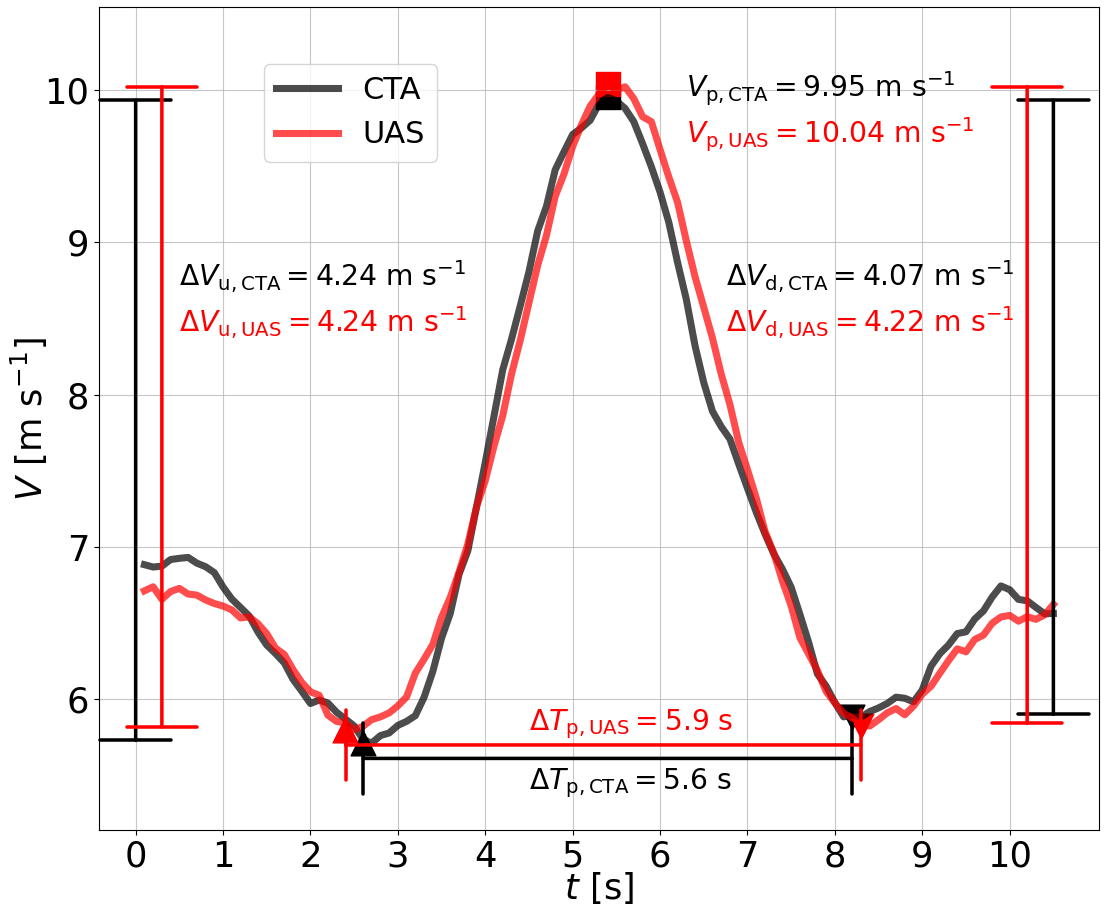
Figure 2Exemplary wind speed time series comparison of a gust measured by the UAS and the CTA. The black line represents the time series measured with the CTA; the red line represents the time series measured with the UAS. The maximum speed differences in the gust ΔVu and ΔVd are shown for the increasing and decreasing speed in the gust passage. Vp denotes the maximum wind speed of the gust and ΔTp the time difference between the downward peaks of the gust.
From the set of resulting gust profiles, the most and least pronounced gusts are selected for the different wind speed ranges. This yields the gusts listed in Table A2, from which 10 repetitions were measured in each flight.
The duration of a single gust is 10.5 s. We analyze the wind measurement for the initial and maximum wind speeds, V0 and Vp = V0+Vg, via Eq. (3) and the time response by comparing the time delta ΔT between the downward peaks registered by the UAS and the CTA,
3.2.4 Velocity steps
Similar to the analysis of the measurement in gusts, tests are performed in velocity steps (Fig. 3) to verify the response time behavior and the accuracy of the wind measurement in abrupt changes in the flow condition. For this study the flow generation configurations from Neuhaus et al. (2021) are used. Therefore, the following setups for the initial velocity V0 and the step velocity Vdu, which lie within the flight envelope of the UAS, are used (Table A3). For the step amplitudes 7 and 10 m s−1, 10 repetitions were performed, and for the step amplitude of 5 m s−1, a total of 20 repetitions were performed. Each repetition, as shown in Fig. 3, lasts 40 s. They consist of one upward and one downward velocity step with equal duration of the intervals of constant velocity between the steps. In order to measure the time response, the start time of the step and the final time when the target wind speed is reached need to be detected from the time series. The starting points Tu,0 and Td,0 of the upward and downward steps are defined from the most extreme gradients in the time series:
The final points in time of the steps Tu,1 and Td,1 are defined when 90 % of the delta between the measured higher and lower stationary velocities Vh and Vl are reached:
The measured upward and downward velocity steps ΔVu and ΔVd, as well as the step times ΔTu and ΔTd, are defined through the following points in the time series:
We analyze the timing accuracy by comparing these time deltas using Eq. (5). The accuracy of measurements by the UAS and the CTA of Vl and Vh are analyzed via Eq. (3), and the accuracy of the upward and downward velocity steps ΔVu and ΔVd are analyzed using Eq. (14),
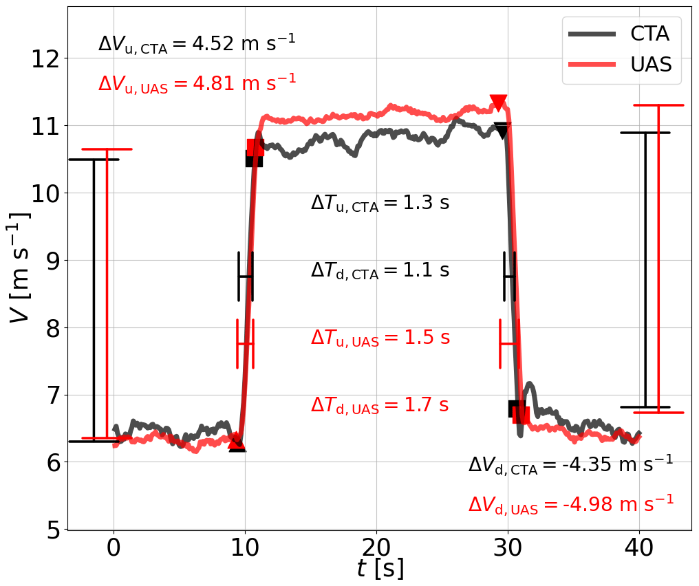
Figure 3Exemplary wind speed time series comparison of velocity steps measured by the UAS and CTA. The black line represents the time series measured with the CTA; the red line represents the time series measured with the UAS. The maximum speed differences in the velocity step passage ΔVu and ΔVd are shown for the upward and downward velocity steps, respectively. The time differences ΔTu and ΔTd denote the respective durations for these steps calculated according to Eqs. (6)–(13).
3.2.5 Turbulence
To verify the ability of the UAS measurement to resolve turbulence, we perform experiments with different turbulence intensities and mean wind speeds. For this, we use two programs for the active grid's flap motion control, one for generating higher turbulence intensity and one for lower turbulence intensity. We run constant wind speed in the wind tunnel and execute the programs. In addition, the wind tunnel controller can use the speed of the wind tunnel's fans. This enables us to achieve higher length scales and intensities of turbulence. The setups of preset wind speed V0 and turbulence intensity I are listed in Table A4. The setting V(t) means that no constant background wind speed was set, but the wind tunnel fans were included in the turbulence generation. This turbulence generated with the active grid is reproducible from a statistical point of view and is therefore referred to as statistical turbulence.
Each measurement run for statistical turbulence has a duration of 600 s. By examining the power spectral density (PSD) of the turbulence, we investigate the maximum resolvable frequency f, as well as the determination of the turbulence intensity I (Eq. 16) with the standard deviation σ (Eq. 15) of all values Vi of the wind speed time series. The RMSE in the determination of the turbulence intensity ϵI is calculated and analyzed with a dependence on the variance σ2 (Eq. 17).
4.1 Calibration
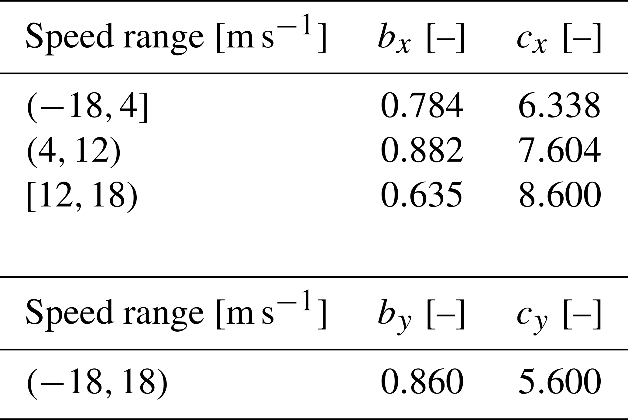
We have found that higher accuracy can be attained, particularly at high and low speeds, if we use dedicated calibration coefficients for different speed ranges in the longitudinal direction, as listed in Table 2.
Table 2Calibration coefficients bi and ci as used in Eq. (1) for different speed ranges.
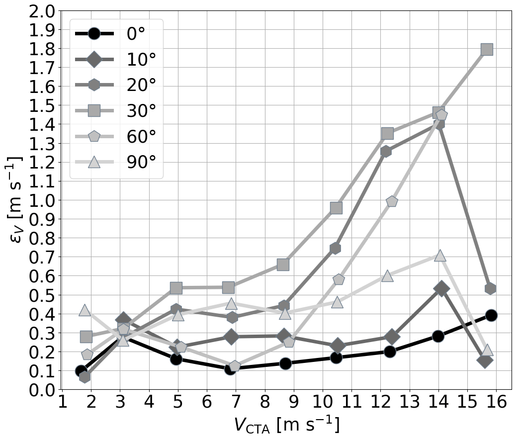
4.2 Angles of sideslip
By applying these coefficients, we obtain the RMSE for the wind speed measurement ϵV for each speed step and each AoS (see Fig. 4). At 0° AoS, ϵV is below 0.4 m s−1 and below 0.2 m s−1 in the wind speed range 5 … 12 m s−1. For all measured wind speeds, the overall ϵV yields 0.19 m s−1. At an AoS of 90° and wind speeds up to 11 m s−1, ϵV is below 0.5 m s−1 and reaches a maximum of about 0.7 m s−1 at a wind speed of 14 m s−1. For the other angles, especially 20, 30, and 60°, the error is significantly higher, particularly above wind speeds of 9 m s−1.
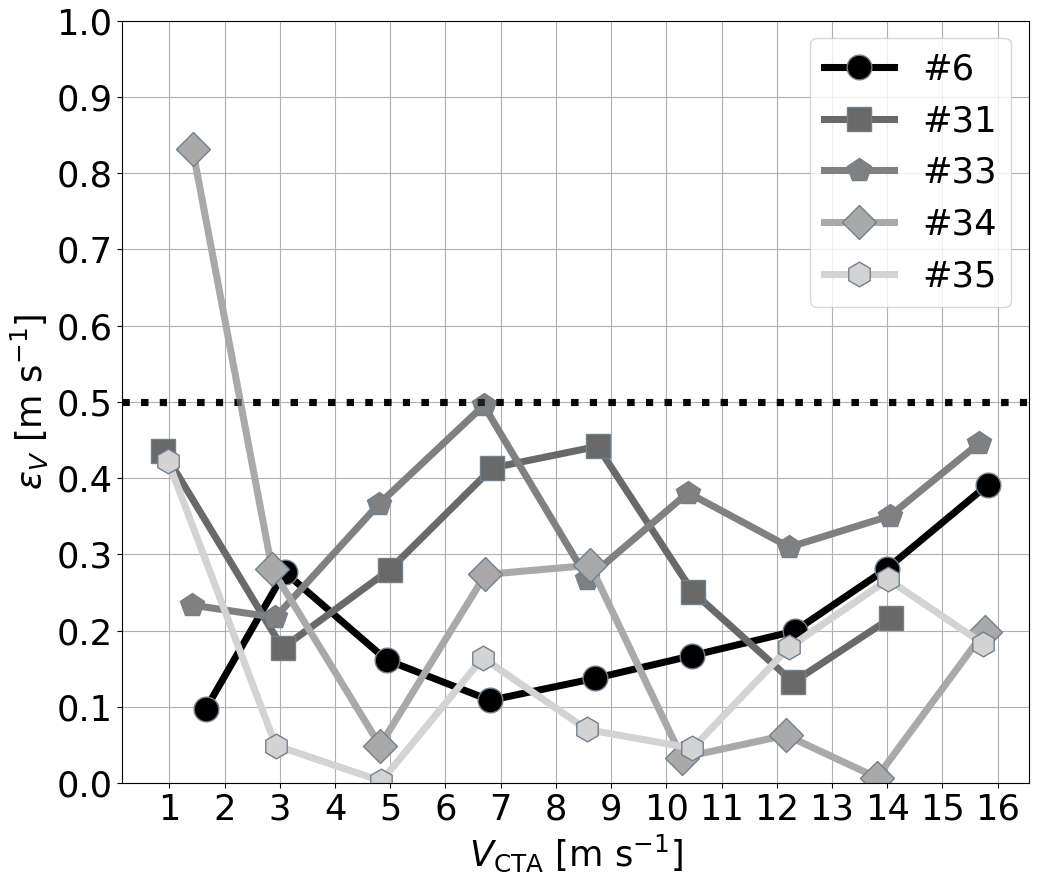
4.3 Portability
Applying the calibration coefficients to other UASs in the fleet, we again determine ϵV for each wind speed step (see Fig. 5). Throughout the fleet, ϵV is below 0.5 m s−1 for all velocity ranges, except for one data point: at a wind speed of 1.4 m s−1, UAS no. 34 shows an error of over 0.8 m s−1 compared to the CTA. Why UAS no. 34 experienced this acceleration despite the low wind speed was likely due to a random error in the experimental setup and cannot be reproduced at this point.
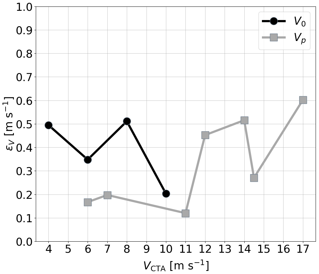
4.4 Gusts
For the gust measurements, we analyze both the accuracy of wind speed measurement and the response time behavior. The RMSE for the response time behavior ϵΔT is 4.5 × 10⁻¹ s with a reference sensor standard deviation of 3.6 × 10⁻¹ s. The RMSE of the wind speed measurement over the different speed ranges is shown in Fig. 6. For all V0 and for Vp up to 13.5 m s−1, ϵV is ≤ 0.5 m s−1.
4.5 Velocity steps
For the velocity steps, just like for the gusts, we investigate the accuracy of wind speed measurement and response time. Here ϵΔT for ΔTu and ΔTd is 7.1 × 10⁻¹ s with a reference sensor standard deviation of 6.5 × 10⁻¹ s. The RMSEs of the wind speed measurements are shown in Fig. 7. The ϵV for Vl is about 0.8 m s−1 and for Vh it is ≤ 0.3 m s−1. A significant increase in the error can be observed for ΔVu and ΔVd with ϵΔV of almost 1.0 m s−1 and over 1.3 m s−1, respectively.
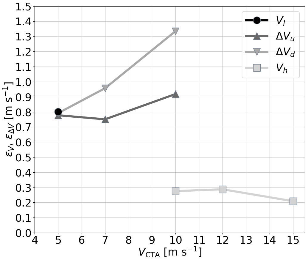
Figure 7RMSEs of UAS-based speed measurements ϵV and ϵΔV in velocity steps over preset wind speed VCTA. The RMSEs are calculated according to Eqs. (3) and (14), respectively. The different lines represent different speed sections of the time series, i.e., the measured higher stationary wind speed Vh, the lower stationary wind speed Vl, the upward velocity step ΔVu, and the downward velocity step ΔVd.
4.6 Turbulence
For the measurements with statistical turbulence, we investigate the variance, the turbulence intensity, and the resolvable scales. From the PSD it can be observed that neither the spectra measured by the CTA nor those measured by the UAS follow the Kolmogorov model over the entire frequency range (Fig. 8). Only in the high-frequency range from 101 Hz and also in the low-frequency range for the V(t) setup do the spectra follow the Kolmogorov model. The transition range deviates in all measurements. This is not of any further concern within this study, since the consistency of the UAS with the CTA and not with the model is investigated. In general, the spectra of the UAS and CTA measurements agree well; the R2 value of 0.886 at a p value of 2 × 10⁻¹⁰ shows a very strong correlation between the variances and . However, if the variance of the turbulence is below approx. 0.5 m2 s−2, the spectra diverge at about 2 Hz. For 0.3 m2 s−2 and below, there is a divergence at about 1 Hz.
This result can also be identified in Fig. 9: the correlation between CTA and UAS measurements changes below 0.5 m2 s−2 and differs strongly below 0.3 m2 s−2 compared to the higher variance ranges. Furthermore, a bias in the form of a systematic underestimation of the UAS values can be observed. This occurs when the variance of the reference measurement is determined over all frequencies up to the maximum frequency fm,CTA that can be resolved by the CTA. However, if the variance of the CTA is only calculated up to the maximum frequency fm,UAS measured by the UAS, this bias does not occur.
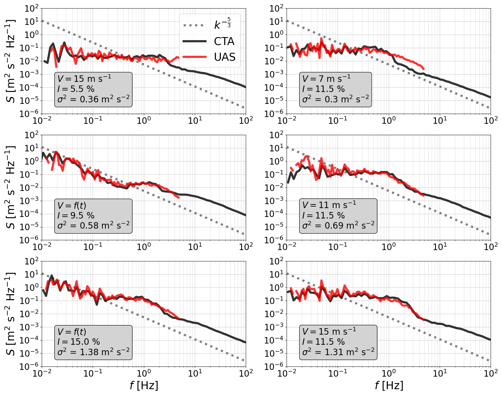
Figure 8Comparison of exemplary PSD of the wind speed S determined via UAS and CTA measurements at different preset wind speeds V and turbulence intensities I, with the respective variance σ2 indicated. The dotted grey line represents the spectrum following the Kolmogorov power law, the black line represents the PSD derived from CTA measurements, and the red line represents the PSD derived from UAS measurements. The variance is calculated according to Eq. (15), and the turbulence intensity is defined according to Eq. (16). The spectra are processed with bin averages in the frequency space to decrease the noise.
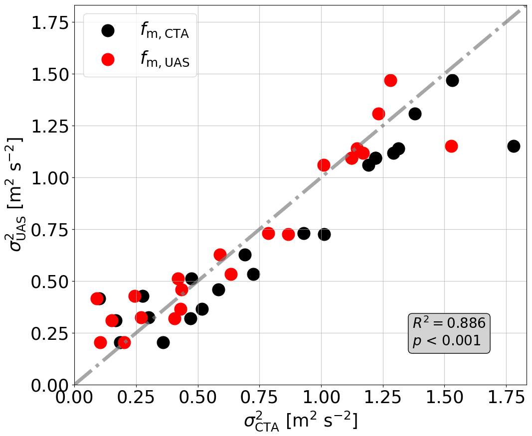
Figure 9Comparison of the variances σ2 obtained via the measurements of UAS and CTA, with determined according to Eq. (15) with the measurement frequency of the CTA fm, CTA (black dots) and with the measurement frequency of the UAS fm, UAS (red dots) as the maximum frequencies.
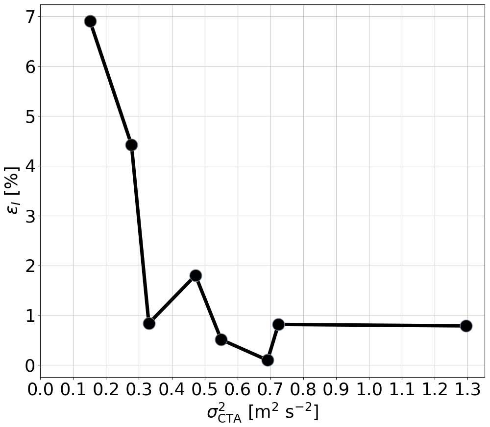
This fact is also reflected in the RMSE for measurement of the turbulence intensity (see Fig. 10): ϵI increases significantly at a variance of less than 0.3 m2 s−2. This effect is due to the signal-to-noise ratio of the accelerometer measurements and self-induced vibrations by the UAS, which are stronger than the atmospheric flow signal below certain energy levels.
Our experiments show that for measurements carried out using UASs from the SWUF-3D fleet, the RMSE of wind speed along the wind direction exceeds 0.5 m s−1 only in ranges that are close to the extrema of accelerations and wind speeds. Generally, the determined accuracy of the UAS measurements has to be assessed considering the uncertainty in wind speeds in the wind tunnel test section as described in Sect. 2.2 and the uncertainties in the CTAs mentioned in Sect. 2.3.
For the wind measurements, we observe accuracy that is comparable to the results in other studies: González-Rocha et al. (2023) obtain an RMSE of 0.6 m s−1 for time averages of about 2 min intervals in hover flight and an RMSE of 2.5 m s−1 in ascending vertical flight. In their comparisons for the rigid-body method, González-Rocha et al. (2019) find an RMSE of 0.4 to 0.7 m s−1. When time averaged over 20 s, in the measurements of Neumann and Bartholmai (2015) the RMSE for the wind speeds in an outdoor flight are 0.6 m s−1 for hover and 0.36 m s−1 for motion flight; in the wind tunnel experiments of Neumann et al. (2012) the RMSE is 0.6 m s−1. It should be emphasized that Neumann and Bartholmai (2015) measured at AoSs of 0, 45, and 90° to the main flow direction and up to 8 m s−1 wind speed and found that there were no significant differences in the wind measurement due to the heading of their system. In contrast to this, in our investigations within this speed range, the accuracy at different AoSs is sufficiently low but differs significantly for various yaw angles. Brosy et al. (2017) obtained an RMSE of 0.3 m s−1 in free-field calibration of their system up to about 6 m s−1 wind speed and an RMSE of 0.7 m s−1 in time series smoothed with a 10 s moving average in flight tests. Also using 10 s periods, the RMSE for the measurements by Palomaki et al. (2017) is 0.32 ± 0.17 m s−1. Simma et al. (2020) achieve an RMSE between 0.26 and 0.29 m s−1 for horizontal wind estimates. The RMSE in the measurements of Segales et al. (2020) is 0.77 m s−1. Of particular interest is that Wetz and Wildmann (2023) report an RMSE of 0.25 m s−1 for the mean wind speed with the calibration coefficients from Wetz et al. (2021) since here measurements are performed with the same setup as in our investigations but with the coefficients from calibration in the free field. However, when applied to the validation data from the wind tunnel, these calibration values have a significantly higher error than the calibration coefficients determined in the wind tunnel. Also, the measurements in Wetz and Wildmann (2023) are performed in mean wind speeds of 6 … 12.5 m s−1. Both in the former and in the new calibration, the measurement uncertainties are lowest in this speed range. The measurements in the wind tunnel, in contrast, have been carried out at significantly lower and higher wind speeds, which contribute to the overall increased RMSE. Nevertheless, there is agreement in the turbulence measurement: Wetz and Wildmann (2022) also find variances of 0.3 m2 s−2 and 2 Hz as the lower limits of resolvable turbulence and temporal resolution. Deviations from the reference in the turbulence measurement at the higher frequencies are also found by Shelekhov et al. (2022) but are not as pronounced as in the cases presented here.
In general, our measurement setup exhibits some deficiencies: the optical flow sensor that was used does not maintain the position without error but causes a slight movement in the horizontal plane. This leads to uncertainties, as the movement affects the wind measurements and cannot be compensated for due to the unavailability of GNSS. Since the sensor itself could be pinpointed as the source of this error, the use of a different optical flow system can potentially eliminate this inaccuracy. Some of the measurements carried out could not be used for the analyses in this paper as errors in the CTA data occurred.
We found throughout the process of calibration that different calibration coefficients for different velocity ranges in the longitudinal direction achieved higher accuracy for the wind speed measurements. This, in addition to applying coefficients from the lateral calibration, leads to good results at different AoSs. The accuracy at 0° AoS is best and similarly good at 10°, while measurement errors at AoSs of 20 … 60° are higher than desired, especially at high wind speeds. This shows that it is appropriate and essential to operate in weather vane mode. Analyses of deviations between UAS headings and measured wind direction from actual field measurements as presented in Wetz and Wildmann (2023) show that the directional error is always below 30° for velocities starting at 2 m s−1, is typically below 20° for wind speeds above 4 m s−1, and generally decreases with higher wind speeds (see Fig. B3). This means that AoSs occurring at different wind speeds and inaccuracies in the wind speed measurement as a result of the AoS counteract each other. The calibration coefficients obtained are portable to other UASs in the fleet without a significant loss in accuracy. The aforementioned single outlier in the calibration of UAS no. 34 is not caused by putative limitations of the portability of coefficients but by a random experimental error during that flight.
When measuring gusts, the RMSE of the stationary speeds is slightly above the RMSE of calibration flights. During these flight phases, the position corrections were carried out, and their impact on the wind measurement cannot be corrected completely. Also, the RMSE for very high velocities at the peak of the gust profile is slightly above that of calibration flights. The RMSE for the time response of 4.5 × 10⁻¹ s is satisfactory in this regard, especially with respect to the standard deviation of the CTA of 3.6 × 10⁻¹ s, the inhomogeneity in the wind field, and the distortions of the experienced gust duration at the UAS due to its motion. However, due to the positional drift, these results should be taken with some caution, as the position of the UAS with respect to the CTA may have changed within the time frame considered, which may also distort the timescale in which gust characteristics reach the UAS.
In the same manner as for the gusts, the RMSE of the stationary speeds is found to be higher for the velocity steps than for calibration flights, which is also due to position corrections during these phases. The error in the upward and downward velocity steps is high but also within the limits when this is related to the flow condition: at a velocity drop of 10 m s−1 within approx. 1.5 s, the RMSE of approx. 1.3 m s−1 is still acceptable for our applications.
For the turbulence measurement, the RMSE for the wind speed is slightly higher than for the calibration flights due to the positional drift. As mentioned above, the turbulence spectra measured by CTA and UAS both deviate from the Kolmogorov power law and exhibit a characteristic hump at approximately 1 Hz. This is of minor importance for the analyses of this work; the agreement of the spectra and the accuracy in measuring turbulence intensity are the important points of relevance. This is found to be satisfactory for variances higher than 0.5 m2 s−2 and for frequencies up to 2 Hz at variances above 0.3 m2 s−2. A systematic bias between variances obtained via UAS and CTA occurs, which is caused by the different frequency resolutions and the missing energy of the small scales that cannot be measured by the UAS. Nevertheless, the very strong correlation between the measured variances of UAS and CTA indicate a consistent measurement quality across a major range of variances. However, the goal is still to resolve smaller-scale turbulence, which probably requires a smaller airframe and smaller propellers for the UAS, which is in turn associated with lower maximum takeoff weight and thus smaller batteries, reducing the maximum flight time.
Nonetheless, due to the dataset and the properties of the turbulent flow measured in this work, additional turbulence measurements are necessary in the future to enable a more detailed quantification of the turbulence estimation capabilities of the SWUF-3D fleet. This requires the generation of statistical turbulence with PSDs not exhibiting the aforementioned hump but with closer agreement to the slope or at least some distinctly characteristic slope that is clearly discernible from white noise. This is essential in order to also verify a potentially more general measurable minimum at those frequency ranges. This cannot be definitively deduced from the data available so far.
In this work, we successfully performed advanced calibration of our wind measurement using UASs under laboratory conditions in a wind tunnel. Using the active grid of the wind tunnel, we were able to verify the accuracy of the wind measurement using the newly obtained calibration coefficients in a broad variety of flow conditions.
By means of the measurement accuracies at different AoSs in steady wind speeds, we have demonstrated the necessity of the weather vane mode for our system and showed that measurements are reliable even in case of delayed response or errors in the yaw control. Without any angle of sideslip, the uncertainty remains below 0.4 m s−1, but as soon as the AoS increases above 20°, a significant increase in uncertainty is observed. Errors of more than 0.7 m s−1 are found, especially above wind speeds of 9 m s−1.
By determining the measurement accuracy using the identical calibration coefficients on other UASs in the fleet, we were able to demonstrate the portability of these coefficients to equivalent systems. For the measurements of all evaluated UASs, the RMSE is below 0.5 m s−1. This allows for further upscaling of the fleet without the need to perform individual wind tunnel calibrations on new UASs of this type.
Based on the different measurement scenarios using the active grid, we were able to verify the measurement accuracy in more complex and dynamic flow conditions. For measurements in gusts, the maximum RMSE of about 0.6 m s−1 was obtained at 17 m s−1 wind speed. Furthermore, steady winds were also measured directly after abrupt velocity steps with an acceptable error (the respective lower velocities with an error of 0.8 m s−1 and the upper ones with less than 0.3 m s−1). For the measurements of extreme wind speed changes, we observed a significant increase in the RMSE for the speed measurement. Here, the RMSE for the response time is 7.1 × 10⁻¹ s, and for the gust time measurement it is 4.5 × 10⁻¹ s. On the basis of measurements in flows with statistical turbulence, we were able to detect limits for the resolution of turbulent winds. Generally, we achieve a high level of agreement in the measurement of turbulence parameters between UASs and the reference CTA, but we observed a significant increase in the measurement errors for absolute variances below 0.3 m2 s−2. In this variance range, the PSD of the UAS and CTA diverge at frequencies above approx. 1 Hz. Between 0.3 and 0.5 m2 s−2, this maximum frequency for accurate turbulence measurement is about 2 Hz, and no systematic divergence has been found at higher variances. However, due to the properties of the turbulence spectra of generated flows by the active grid, the need to investigate further limits of turbulence resolution in terms of variance and frequency and their interactions remains, both within and beyond the value ranges considered in this work.
To summarize, calibration along the main axes of the UAS is not fully sufficient in all inflow directions without the weather vane mode. Based on the validation with other UASs in the fleet, the hypothesis of portability was confirmed. The validation in gusts, velocity steps, and statistical turbulence showed that with the calibration method in stationary wind speeds it is possible to reliably measure highly dynamic flows with the UAS. Further studies with more extensive and detailed turbulence analysis in the wind tunnel will also include other airframes with different rotor sizes. In addition, there is a need to integrate the vertical wind component (Wildmann and Wetz, 2022) into the type of analysis presented in this paper, ideally along with calibration under similar laboratory conditions. Since the work presented here is part of the SWUF-3D fleet research, it is important to integrate the established accuracy into the analysis of uncertainties in spatially distributed fleet measurements, which needs to be validated via measurements in field experiments.
Table A1Measurement presets with various absolute angles of sideslip , maximum tested wind speeds Vmax, the averaging period Ts for the wind speeds, and the number of measurements r carried out with the respective preset.
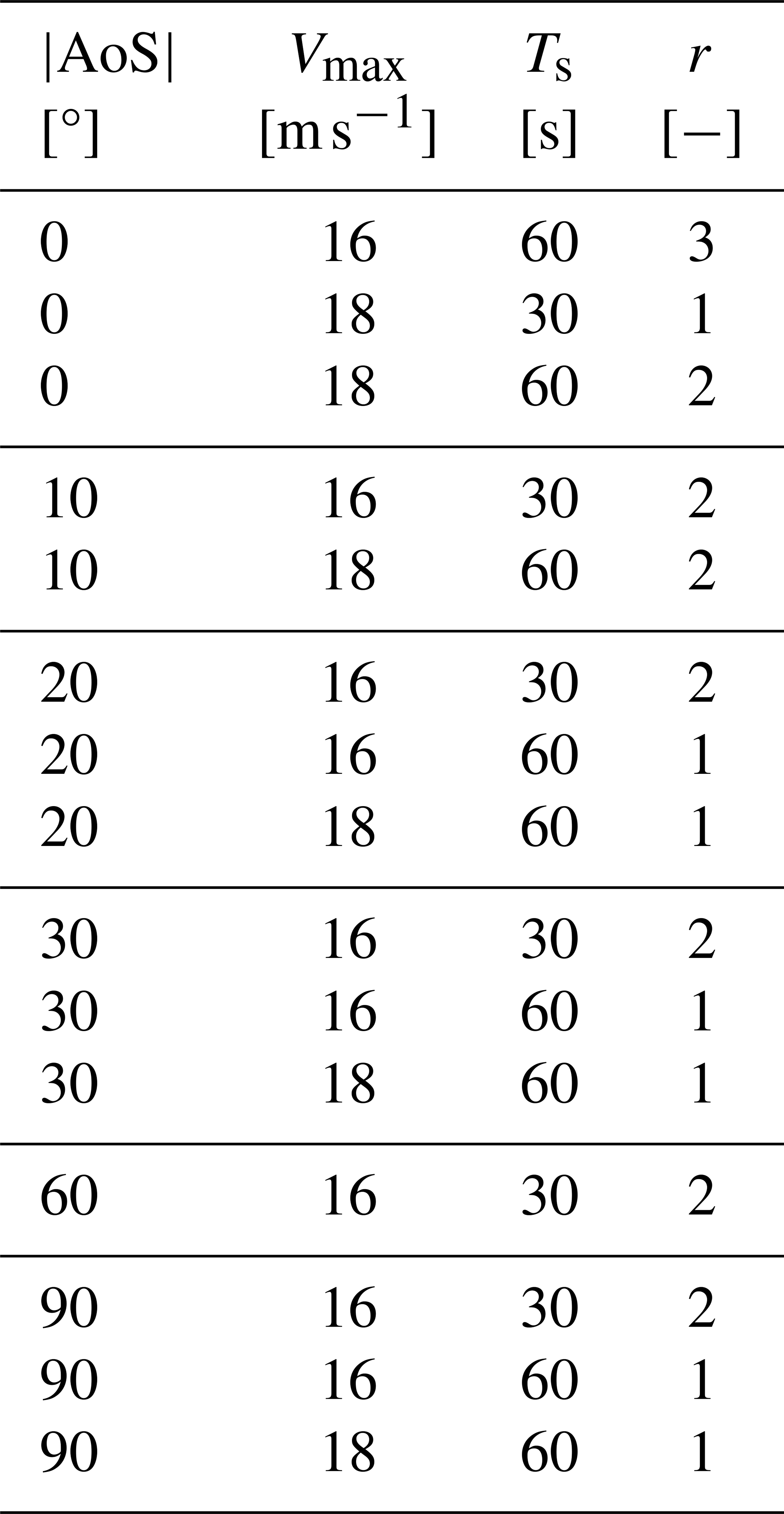
Table A2Measurement presets for gusts with the initial wind speed V0 and the wind speed amplitude Vg.
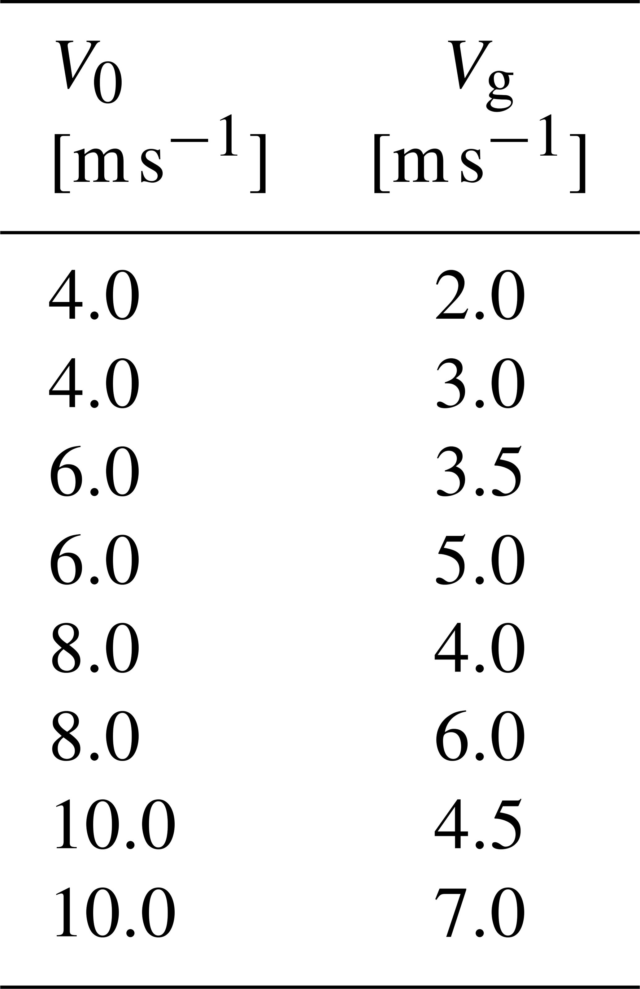
Table A3Measurement presets for velocity steps with the lower wind speed V0 and the upward and downward step velocity Vdu.
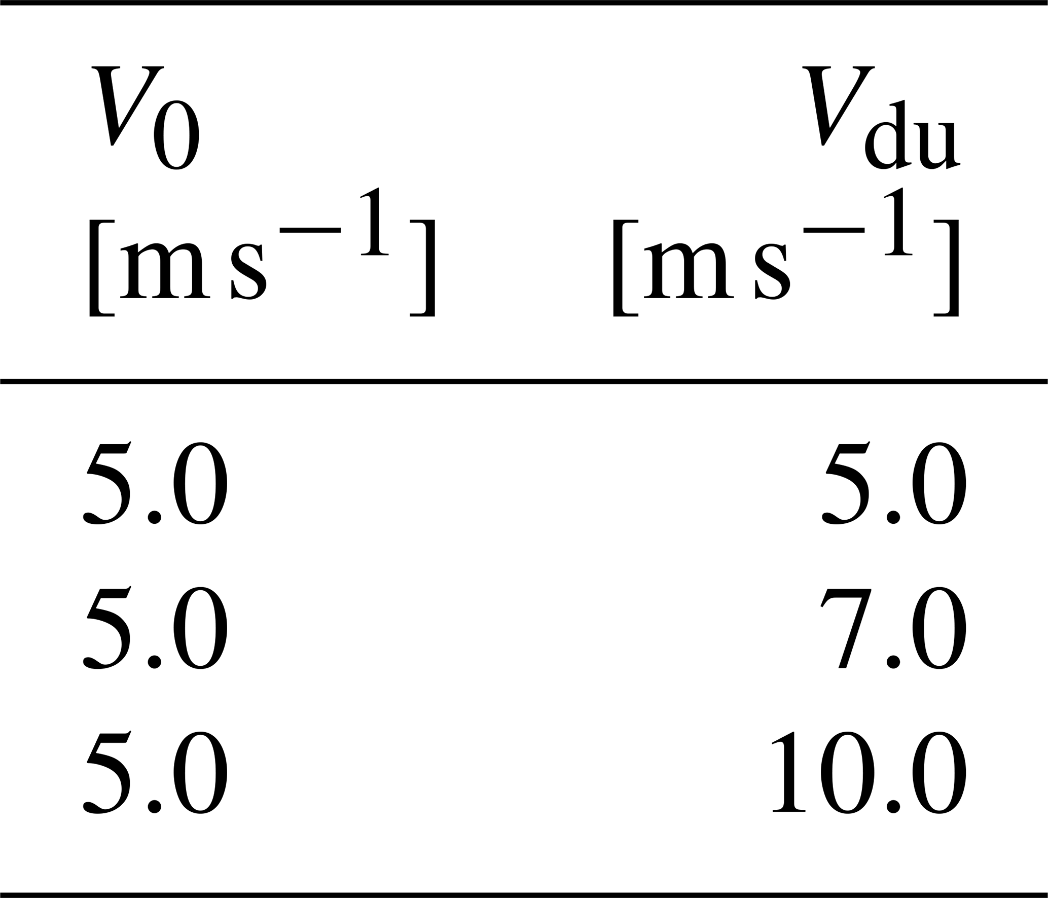
Table A4Measurement presets for statistical turbulence with the fan wind speed V0, the turbulence intensity I according to Eq. (16), and the number of measurements r carried out with the respective preset.
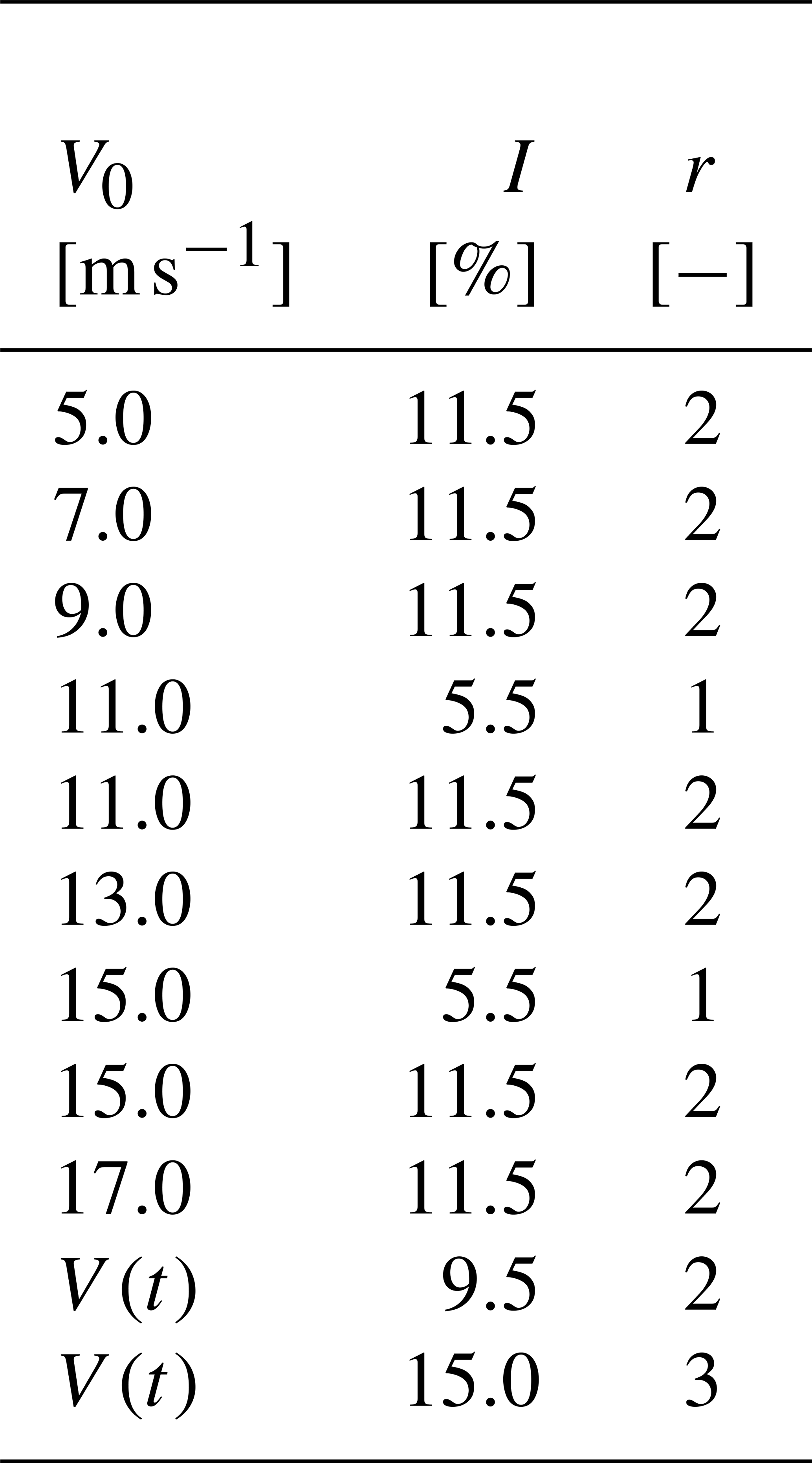
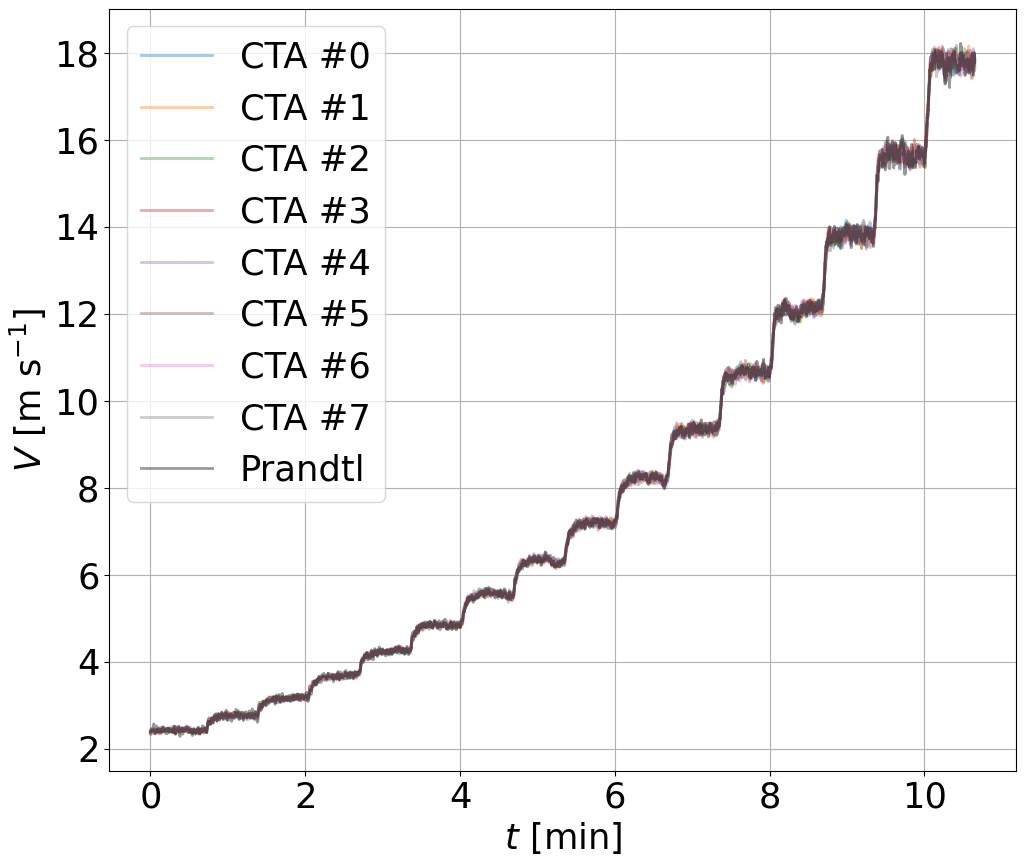
Figure B1Comparison of the time series of the logarithmically increasing wind speeds V measured with the individual CTAs and the Prandtl probe without a UAS flying during the measurement. The different lines represent different sensors.
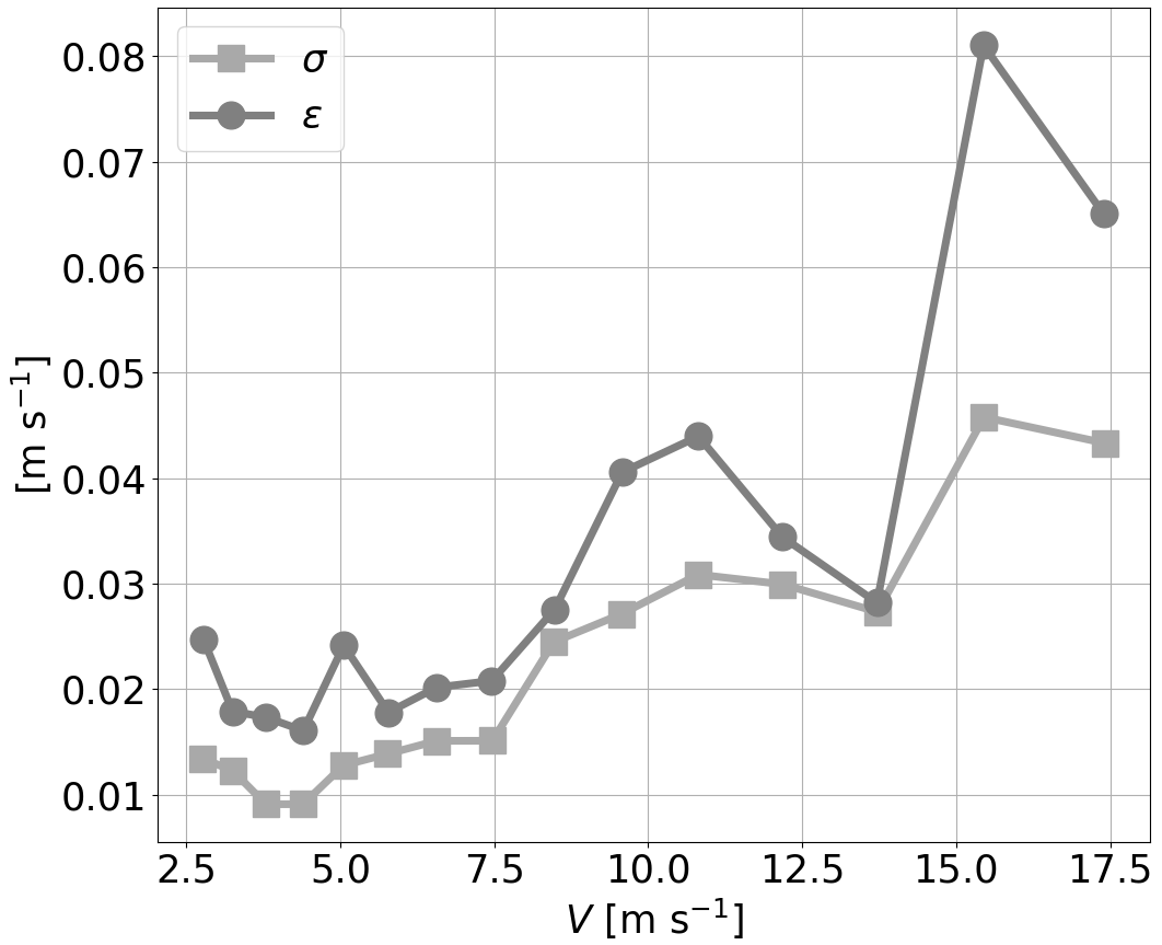
Figure B2Standard deviation of the CTAs σ and the RMSE of the CTAs to the Prandtl probe ϵ for the wind speed measurements without a UAS flying during the measurements, which were performed twice each day. The standard deviation is calculated according to Eq. (15), and the RMSE is derived according to Eq. (3).
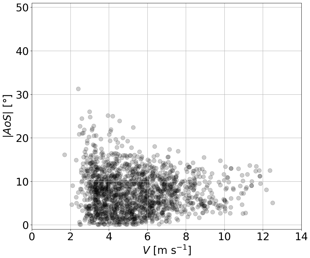
Figure B3Absolute mean angle of sideslip over mean measured wind speed V for 60 s segments of 209 UAS measurement flights in the open field with an average flight duration of over 8 min each.
| ABL | Atmospheric boundary layer |
| AoS | Angle of sideslip |
| bx, by | Exponential calibration coefficients |
| cx, cy | Linear calibration coefficients |
| CTA | Constant temperature anemometer |
| f | Frequency |
| Fw | Wind force |
| GNSS | Global navigation satellite system |
| I | Turbulence intensity |
| PSD | Power spectral density |
| r | Number of runs |
| R | Rotation matrix |
| RMSE | Root-mean-square error |
| S | PSD |
| t | Time |
| Ts | Time for which wind speeds are kept constant for calibration |
| u | Longitudinal wind speed component |
| UAS | Uncrewed aerial system |
| v | Lateral wind speed component |
| V | Wind speed vector |
| V0 | Inertial wind speed of gust, lower wind speed of velocity step, and fan wind speed for statistical turbulence |
| Vdu | Wind speed aimed at the upward and downward velocity step |
| Vg | Targeted gust velocity amplitude |
| Vh | Higher wind speed between velocity steps |
| Vl | Lower wind speed between velocity steps |
| Vp | Maximum speed in gust passage |
| Velocity in the longitudinal direction of the geodetic coordinate system detected by the GNSS | |
| Velocity in the lateral direction of the geodetic coordinate system detected by the GNSS | |
| ΔTd | Duration of the downward velocity step |
| ΔTg | Duration of the gust between downward peaks |
| ΔTu | Duration of the upward velocity step |
| ΔVd | Wind speed of the downward velocity step and gust |
| ΔVu | Wind speed of the upward velocity step and gust |
| ϵI | RMSE of turbulence intensity |
| ϵV | RMSE of wind speed |
| ϵΔT | RMSE of time deltas |
| ϵΔV | RMSE of wind speed deltas |
| θ | Pitch angle |
| σ | Standard deviation |
| σ2 | Variance |
| ϕ | Roll angle |
| ψ | Yaw angle |
The data is available at https://doi.org/10.5281/zenodo.10047738 (Kistner et al., 2023).
JK wrote the main paper and performed the calibrations and data analysis. The experiment was conducted by JK. NW provided the algorithm to measure wind with the quadrotor, was involved in the experiment, and contributed to the writing of the paper. LN provided the wind tunnel setups and wrote the description of the wind tunnel.
The contact author has declared that none of the authors has any competing interests.
Publisher’s note: Copernicus Publications remains neutral with regard to jurisdictional claims made in the text, published maps, institutional affiliations, or any other geographical representation in this paper. While Copernicus Publications makes every effort to include appropriate place names, the final responsibility lies with the authors.
We thank Tamino Wetz and Michael Hölling for their assistance during the wind tunnel measurements. Andreas Marsing and Gerhard Kilroy reviewed the manuscript internally and we thank them for their valuable comments. We also thank the two anonymous reviewers for their helpful comments on an earlier version of this paper. Pixhawk is a trademark of Lorenz Meier.
This research is part of the project ESTABLIS-UAS and has been supported by the HORIZON EUROPE European Research Council (grant no. 101040823).
The article processing charges for this open-access publication were covered by the German Aerospace Center (DLR).
This paper was edited by Peter Alexander and reviewed by two anonymous referees.
Brosy, C., Krampf, K., Zeeman, M., Wolf, B., Junkermann, W., Schäfer, K., Emeis, S., and Kunstmann, H.: Simultaneous multicopter-based air sampling and sensing of meteorological variables, Atmos. Meas. Tech., 10, 2773–2784, https://doi.org/10.5194/amt-10-2773-2017, 2017. a, b
González-Rocha, J., Woolsey, C. A., Sultan, C., and Wekker, S. F. J. D.: Sensing Wind from Quadrotor Motion, J. Guid. Control Dynam., 42, 836–852, https://doi.org/10.2514/1.g003542, 2019. a, b
González-Rocha, J., Bilyeu, L., Ross, S. D., Foroutan, H., Jacquemin, S. J., Ault, A. P., and Schmale, D. G.: Sensing atmospheric flows in aquatic environments using a multirotor small uncrewed aircraft system (sUAS), Environmental Science: Atmospheres, 3, 305–315, https://doi.org/10.1039/d2ea00042c, 2023. a, b
Hattenberger, G., Bronz, M., and Condomines, J.-P.: Estimating wind using a quadrotor, Int. J. Micro Air Veh., 14, 175682932110708, https://doi.org/10.1177/17568293211070824, 2022. a, b
IEC 2019: Wind energy generation systems - Part 1: Design requirements, Standard IEC61400-1:2019, International Electrotechnical Commission, Geneva, Switzerland, ISBN 978-2-8322-7972-4, 2019. a
ISO 2007: Meteorology - Wind measurements - Part 1: Wind tunnel test methods for rotating anemometer performance, Standard ISO17713-1:2007, Beuth Verlag, Berlin, Germany, https://doi.org/10.31030/9866977, 2007. a
Kistner, J., Wildmann, N., and Neuhaus, L.: High resolution wind speed measurements with multicopters of the SWUF-3D UAS fleet - calibration and verification in a wind tunnel with active grid, Zenodo [data set], https://doi.org/10.5281/zenodo.10047738, 2023. a
Kröger, L., Frederik, J., van Wingerden, J.-W., Peinke, J., and Hölling, M.: Generation of user defined turbulent inflow conditions by an active grid for validation experiments, J. Phys. Conf. Ser., 1037, 052002, https://doi.org/10.1088/1742-6596/1037/5/052002, 2018. a
Marino, M., Fisher, A., Clothier, R., Watkins, S., Prudden, S., and Leung, C. S.: An Evaluation of Multi-Rotor Unmanned Aircraft as Flying Wind Sensors, Int. J. Micro Air Veh., 7, 285–299, https://doi.org/10.1260/1756-8293.7.3.285, 2015. a
Molter, C. and Cheng, P. W.: ANDroMeDA - A Novel Flying Wind Measurement System, J. Phys. Conf. Ser., 1618, 032049, https://doi.org/10.1088/1742-6596/1618/3/032049, 2020. a
Neuhaus, L., Hölling, M., Bos, W. J., and Peinke, J.: Generation of Atmospheric Turbulence with Unprecedentedly Large Reynolds Number in a Wind Tunnel, Phys. Rev. Lett., 125, 154503, https://doi.org/10.1103/physrevlett.125.154503, 2020. a
Neuhaus, L., Berger, F., Peinke, J., and Hölling, M.: Exploring the capabilities of active grids, Exp. Fluids, 62, 130, https://doi.org/10.1007/s00348-021-03224-5, 2021. a, b
Neumann, P., Asadi, S., Lilienthal, A., Bartholmai, M., and Schiller, J.: Autonomous Gas-Sensitive Microdrone: Wind Vector Estimation and Gas Distribution Mapping, IEEE Robot. Autom. Mag., 19, 50–61, https://doi.org/10.1109/mra.2012.2184671, 2012. a, b
Neumann, P. P. and Bartholmai, M.: Real-time wind estimation on a micro unmanned aerial vehicle using its inertial measurement unit, Sensor. Actuator. A-Phys., 235, 300–310, https://doi.org/10.1016/j.sna.2015.09.036, 2015. a, b, c
Nolan, P., Pinto, J., González-Rocha, J., Jensen, A., Vezzi, C., Bailey, S., de Boer, G., Diehl, C., Laurence, R., Powers, C., Foroutan, H., Ross, S., and Schmale, D.: Coordinated Unmanned Aircraft System (UAS) and Ground-Based Weather Measurements to Predict Lagrangian Coherent Structures (LCSs), Sensors, 18, 4448, https://doi.org/10.3390/s18124448, 2018. a
Palomaki, R. T., Rose, N. T., van den Bossche, M., Sherman, T. J., and Wekker, S. F. J. D.: Wind Estimation in the Lower Atmosphere Using Multirotor Aircraft, J. Atmos. Ocean. Tech., 34, 1183–1191, https://doi.org/10.1175/jtech-d-16-0177.1, 2017. a, b, c
Platis, A., Siedersleben, S. K., Bange, J., Lampert, A., Bärfuss, K., Hankers, R., Cañadillas, B., Foreman, R., Schulz-Stellenfleth, J., Djath, B., Neumann, T., and Emeis, S.: First in situ evidence of wakes in the far field behind offshore wind farms, Scientific Reports, 8, 2163, https://doi.org/10.1038/s41598-018-20389-y, 2018. a
Rautenberg, A., Allgeier, J., Jung, S., and Bange, J.: Calibration Procedure and Accuracy of Wind and Turbulence Measurements with Five-Hole Probes on Fixed-Wing Unmanned Aircraft in the Atmospheric Boundary Layer and Wind Turbine Wakes, Atmosphere, 10, 124, https://doi.org/10.3390/atmos10030124, 2019. a
The SciPy community: scipy optimize curve fit: https://scipy.github.io/devdocs/reference/generated/scipy.optimize.curve_fit.html (last access: 27 May 2024), 2023. a
Segales, A. R., Greene, B. R., Bell, T. M., Doyle, W., Martin, J. J., Pillar-Little, E. A., and Chilson, P. B.: The CopterSonde: an insight into the development of a smart unmanned aircraft system for atmospheric boundary layer research, Atmos. Meas. Tech., 13, 2833–2848, https://doi.org/10.5194/amt-13-2833-2020, 2020. a, b
Shelekhov, A., Afanasiev, A., Shelekhova, E., Kobzev, A., Tel'minov, A., Molchunov, A., and Poplevina, O.: Low-Altitude Sensing of Urban Atmospheric Turbulence with UAV, Drones, 6, 61, https://doi.org/10.3390/drones6030061, 2022. a, b
Shimura, T., Inoue, M., Tsujimoto, H., Sasaki, K., and Iguchi, M.: Estimation of Wind Vector Profile Using a Hexarotor Unmanned Aerial Vehicle and Its Application to Meteorological Observation up to 1000 m above Surface, J. Atmos. Ocean. Tech., 35, 1621–1631, https://doi.org/10.1175/jtech-d-17-0186.1, 2018. a
Simma, M., Mjøen, H., and Boström, T.: Measuring Wind Speed Using the Internal Stabilization System of a Quadrotor Drone, Drones, 4, 23, https://doi.org/10.3390/drones4020023, 2020. a, b
Thielicke, W., Hübert, W., Müller, U., Eggert, M., and Wilhelm, P.: Towards accurate and practical drone-based wind measurements with an ultrasonic anemometer, Atmos. Meas. Tech., 14, 1303–1318, https://doi.org/10.5194/amt-14-1303-2021, 2021. a
Wang, J.-Y., Luo, B., Zeng, M., and Meng, Q.-H.: A Wind Estimation Method with an Unmanned Rotorcraft for Environmental Monitoring Tasks, Sensors, 18, 4504, https://doi.org/10.3390/s18124504, 2018. a
Wetz, T. and Wildmann, N.: Spatially distributed and simultaneous wind measurements with a fleet of small quadrotor UAS, J. Phys. Conf. Ser., 2265, 022086, https://doi.org/10.1088/1742-6596/2265/2/022086, 2022. a, b, c, d, e, f, g, h, i
Wetz, T. and Wildmann, N.: Multi-point in situ measurements of turbulent flow in a wind turbine wake and inflow with a fleet of uncrewed aerial systems, Wind Energ. Sci., 8, 515–534, https://doi.org/10.5194/wes-8-515-2023, 2023. a, b, c, d
Wetz, T., Wildmann, N., and Beyrich, F.: Distributed wind measurements with multiple quadrotor unmanned aerial vehicles in the atmospheric boundary layer, Atmos. Meas. Tech., 14, 3795–3814, https://doi.org/10.5194/amt-14-3795-2021, 2021. a, b, c, d
Wetz, T., Zink, J., Bange, J., and Wildmann, N.: Analyses of Spatial Correlation and Coherence in ABL Flow with a Fleet of UAS, Bound.-Lay. Meteorol., 187, 673–701, https://doi.org/10.1007/s10546-023-00791-4, 2023. a
Wildmann, N. and Wetz, T.: Towards vertical wind and turbulent flux estimation with multicopter uncrewed aircraft systems, Atmos. Meas. Tech., 15, 5465–5477, https://doi.org/10.5194/amt-15-5465-2022, 2022. a, b
Wildmann, N., Rau, G. A., and Bange, J.: Observations of the Early Morning Boundary-Layer Transition with Small Remotely-Piloted Aircraft, Bound.-Lay. Meteorol., 157, 345–373, https://doi.org/10.1007/s10546-015-0059-z, 2015. a
zum Berge, K., Schoen, M., Mauz, M., Platis, A., van Kesteren, B., Leukauf, D., Bahlouli, A. E., Letzgus, P., Knaus, H., and Bange, J.: A Two-Day Case Study: Comparison of Turbulence Data from an Unmanned Aircraft System with a Model Chain for Complex Terrain, Bound.-Lay. Meteorol., 180, 53–78, https://doi.org/10.1007/s10546-021-00608-2, 2021. a
- Abstract
- Introduction
- System description
- Methods
- Results
- Discussion
- Conclusions
- Appendix A: Verification measurement presets
- Appendix B: Supplementary measurement results
- Appendix C: Nomenclature
- Data availability
- Author contributions
- Competing interests
- Disclaimer
- Acknowledgements
- Financial support
- Review statement
- References