the Creative Commons Attribution 4.0 License.
the Creative Commons Attribution 4.0 License.
 | 30 Aug 2024
Closing the gap in the tropics: the added value of radio-occultation data for wind field monitoring across the Equator
Magdalena Pieler
Gottfried Kirchengast
Globally available and highly vertically resolved wind fields are crucial for the analysis of atmospheric dynamics for the benefit of climate studies. Most observation techniques have problems to fulfill these requirements. Especially in the tropics and in the Southern Hemisphere more wind data are required. In this study, we investigate the potential of radio-occultation (RO) data for climate-oriented wind field monitoring in the tropics, with a specific focus on the equatorial band within ± 5° latitude. In this region, the geostrophic balance breaks down, due to the Coriolis force term approaching zero, and the equatorial-balance equation becomes relevant. One aim is to understand how the individual wind components of the geostrophic-balance and equatorial-balance approximations bridge across the Equator and where each component breaks down. Our central aim focuses on the equatorial-balance approximation, testing its quality by comparison with ERA5 reanalysis data. The analysis of the zonal and meridional wind components showed that while the zonal wind was well reconstructed, it was difficult to estimate the meridional wind from the approximation. However, we still found a somewhat better agreement from including both components in the zonal-mean total wind speed in the troposphere. In the stratosphere, the meridional wind component is close to zero for physical reasons and has no relevant impact on the total wind speed. In general, the equatorial-balance approximation works best in the stratosphere. As a second aim, we investigated the systematic data bias between using the RO and ERA5 data and find it smaller than the bias resulting from the approximations. We also inspected the monthly-mean RO wind data over the full example year of 2009. The bias in the core region of highest quality of RO data, which is the upper troposphere and lower stratosphere, was generally smaller than ± 2 m s−1. This is in line with the wind field requirements of the World Meteorological Organization. Overall, the study encourages the use of RO wind fields for regional-scale climate monitoring over the entire globe, including the equatorial region, and also showed a small improvement in the troposphere when including the meridional wind component in the zonal-mean total wind speed.
- Article
(5320 KB) - Full-text XML
- BibTeX
- EndNote


Globally available upper-air wind profiling information is crucial for the analysis of atmospheric dynamics for the benefit of climate studies, as well as climate models and numerical weather prediction. To determine a wind flow in its full state, wind-sensitive measurements need to ensure a high three-dimensional resolution, global coverage, and frequent observations from the troposphere to the stratosphere (English et al., 2013; Baker et al., 2014; Eyre et al., 2020). However, wind measurements in the free atmosphere, depending on the observing system, lack very often one or more of these requirements.
Stoffelen et al. (2005, 2020) emphasize the need for horizontal resolutions smaller than 10 to 500 km, to follow an atmospheric process in detail from initial small-scale amplitudes to evolving dynamical mesoscale structures. The World Meteorological Organization (WMO) and the Observing Systems Capability Analysis and Review tool (OSCAR) require a vertical resolution of wind information of about 1 km in the troposphere and 2 km in the stratosphere for weather and climate applications, with a wind accuracy of ± 2 m s−1 (see WMO-OSCAR, 2023, https://space.oscar.wmo.int/variables/view/wind_horizontal, last access: 19 August 2024).
Furthermore, well-resolved wind data need to be available over the oceans, tropics, and Southern Hemisphere, where often a measurement gap is present. For example, land surface stations, ships, buoys, and wind scatterometers from satellites provide valuable surface data but lack vertical profiling information. Aircraft and atmospheric motion vectors (AMVs) from geostationary or polar satellites provide a high temporal and horizontal sampling at several heights, but they have distinct limits in accurate vertical geolocation and resolution as well as global representation. Wind profilers, radiosondes, and pilot balloons have a high vertical sampling but provide information primarily at single locations over continents and the Northern Hemisphere. On the other hand, the Atmospheric Dynamics Mission (ADM-Aeolus, operating from August 2018 to July 2023) provided 3D wind profiling with a frequent and high-resolution coverage, filling measurement gaps over the oceans, poles, tropics, and the Southern Hemisphere, up to an altitude of about 20 km. However, it depended on clear-air molecular scattering (no measurements within clouds) and on hydrometeor Mie scattering, which can be particularly tricky at tropical latitudes, due to the high-altitude cloud systems (see also Stoffelen et al., 2005, 2020; Kanitz et al., 2019). Finally, wind information is nowadays also obtained implicitly as part of variational data assimilation (4D-Var) in numerical weather prediction analyses that initialize the forecasts, such as through the geostrophic adjustment and directly through the background error covariances (especially where the geostrophic balance applies) as well as through 4D-Var of humidity and/or ozone-tracing data (Geer et al., 2018; Zaplotnik et al., 2023).
In this respect, a valuable complementary data source comes from exploiting a different satellite-based observation technique, the Global Navigation Satellite System (GNSS) radio-occultation (RO) method. RO provides vertical profiles of geophysical variables such as refractivity, density, pressure, and temperature. A basic introduction to the RO method can be found in Kursinski et al. (1997) and Hajj et al. (2002). The applications range across climate monitoring and climate analysis, numerical weather prediction, and space weather applications (e.g., Healy, 2007; Cucurull, 2010; Foelsche et al., 2009; Anthes, 2011; Steiner et al., 2011).
There are several key advantages of RO data, which could make them a beneficial observation-based data set for (indirect) wind field monitoring. First of all, it provides a multi-satellite, long-term stable, global data set record, with no need for inter-calibration between the missions (Wickert et al., 2001; Anthes et al., 2008; Foelsche et al., 2011a; Angerer et al., 2017; Steiner et al., 2020). In addition, RO provides an all-weather capability, which is a specific advantage in the tropics with large high-altitude cloud systems that can limit other observation systems, such as optical sounders. Furthermore, RO data are a high vertical resolution data set, with resolutions of about 100 m to 200 m in the troposphere, to about 500 m in the lower stratosphere at low-to-middle altitudes, and near 1.5 km from the middle stratosphere towards high altitudes (Schwarz et al., 2017, 2018; Zeng et al., 2019). RO data cover well the (free) troposphere and the stratosphere, with a core region of high quality in the upper troposphere and lower stratosphere (e.g., Zeng et al., 2019; Steiner et al., 2020), having a horizontal resolution of about 200 to 300 km (e.g., Kursinski et al., 1997; Foelsche et al., 2011b). Hence, RO can give additional wind profiling information at higher altitude regions, where other observation-based data sets might only cover the troposphere and lower stratosphere (e.g., radiosondes; Ladstädter et al., 2015; Bodeker et al., 2016).
Traditionally, most RO climate studies concentrate on using the high-quality vertical temperature information (e.g., Li et al., 2023; Ladstädter et al., 2023). With respect to numerical weather prediction, the RO bending angle or refractivity profiles are assimilated in forecasting and reanalysis systems (e.g., Kuo et al., 2000; Cardinali and Healy, 2014; Hersbach et al., 2020). It is important to note in this respect, emphasized in Scherllin-Pirscher et al. (2017), that RO data have the power of vertical geolocation, meaning they provide accurate information on the absolute altitude of a measured air parcel. Hence, RO provides virtually independent information on altitude and pressure fields, also enabling scientists to study an accurate representation of the mass-field-driven wind field circulation. So far, only a few studies have analyzed the option of calculating wind fields from RO geopotential fields on isobaric levels. Scherllin-Pirscher et al. (2014) and Verkhoglyadova et al. (2014) have tested the geostrophic wind approximation, excluding the tropics completely between ± 15° latitude. Healy et al. (2020), on the other hand, tested the zonal equatorial-balance equation around the Equator, studying the utility of RO data in a 5° zonal band in the stratosphere.
In a previous study, Nimac et al. (2023) analyzed the geostrophic approximation on a monthly 2.5° × 2.5° latitude × longitude grid for the ERA5 reanalysis and RO data. It was possible to reproduce the original ERA5 winds fairly well and within the target accuracy of ± 2 m s−1. However, in the region of the jet stream, the difference between the two data sets exceeded this target. Furthermore, over large mountain areas (e.g., Himalayan or Andes region) larger deviations were found, since the ageostrophic contribution grows in importance in such regions with the massive influence of topography. Our study furthermore showed that within the 2007 to 2020 evaluation period the difference between RO and ERA5 became noticeably smaller from 2016 onward, coinciding with an ERA5 observing systems change including, as of 2016, additional information from various sources such as land stations, ships, and buoys. This emphasized the temporal stability of RO data and also points to the high quality of RO data (Steiner et al., 2020). In general, the wind speed estimates performed well towards the tropics up to even ± 5° around the equatorial band. Within the equatorial band, the Coriolis force approaches zero and the singularity starts to dominate. For this physical reason, it is not possible to use the geostrophic approximation to retrieve wind fields over a narrow band around the Equator, leaving a gap in RO wind field computation.
In this study, we aim to close this gap by deriving RO winds across the Equator. While in the important pre-work of Healy et al. (2020) a stratospheric zonal-mean zonal wind field was derived in a 10° equatorial band, we aim to compute latitudinally and longitudinally resolved wind fields with RO data. For this purpose, we investigate the zonal (u) and meridional (v) wind components, as well as total wind speed (V), based on the equatorial-balance equation (Chandra et al., 1990; Scaife et al., 2000; Holton, 2004). The method and the data sets used are introduced in Sects. 2 and 3. In a first step, we assess the quality of the approximation, using monthly ERA5 reanalysis data (Hersbach et al., 2020) on a 2.5° × 2.5° grid as a reference. Here, we compare the original ERA5 wind components and wind speeds to the ones computed from the equatorial-balance approximation (Sect. 4.1). In a second step, we derive the zonal and meridional wind components, as well as total wind speed, for monthly RO climatologies, analyzing the quality and added value of RO wind field products over the equatorial band (Sect. 4.2). Finally, in Sect. 4.3, we test how the equatorial-balanced wind speeds bridge the geostrophic wind speeds across the Equator, closing the gap in the tropics with RO wind data. The summary and conclusions are then given in Sect. 5.
The overarching goal is to collect knowledge from the prior study (Nimac et al., 2023) and this current study to produce a long-term stable global climate RO wind field record, covering the upper troposphere up to the middle stratosphere, at monthly and mesoscale resolutions. In this respect, the added value of RO data can play out, i.e., its unique combination of high vertical resolution, accuracy, and long-term stability (meaning multi-year to multi-decadal stability). The possible applications are numerous: from global climate wind field monitoring to studies of changes in climate-related wind field dynamics.
In general, a wind flow in the free atmosphere can be approximated by geostrophic balance, which equals an exact balance between Coriolis force and pressure gradient force. Friction can be ignored in the free atmosphere, while ageostrophic contributions become generally of higher relevance in the winter hemisphere and also above large mountain areas (e.g., Scaife et al., 2000; Nimac et al., 2023). The geostrophic balance breaks down in the tropics, due to the Coriolis force approaching zero, inducing a singularity in the geostrophic approximation. A solution for the wind equation in the tropics, assuming a steady friction-less flow, is the equatorial-balance equation. In this study, we calculate wind speeds using the geostrophic-balance and equatorial-balance approximations, with the main focus on the latter one. The derivation of RO wind fields, based on the geostrophic approximation, has already been thoroughly validated in a prior study (Nimac et al., 2023). In our analysis, we follow the accuracy requirements specified by the World Meteorological Organization (WMO); see WMO-OSCAR, 2023, https://space.oscar.wmo.int/variables/view/wind_horizontal (last access: 19 August 2024). The WMO provides detailed and differentiated requirements for different spatial and temporal resolutions as well as for different applications (e.g., applications in numerical weather prediction). Since our focus is monthly-averaged mesoscale winds relevant for the description of climate, we use an indicative threshold of wind speed biases smaller than ± 2 m s−1. We further note that the advantage of RO-based long-term wind records is their unique potential of being temporally stable, which is another WMO requirement of stability. Considering monthly-mean wind speeds with an accuracy within ± 2 m s−1, this is roughly consistent with a decadal stability of ± 0.5 , which is the associated WMO-based requirement that we use to evaluate long-term stability (see Nimac et al., 2023).
The equatorial-balance equation. To derive wind fields over the Equator, we follow the formulation of Chandra et al. (1990) and Scaife et al. (2000). The equatorial wind data are derived from geopotential (Φ), given on isobaric levels, resulting in the following formulation for the zonal and meridional wind components, ueb and veb, respectively, over the Equator:
where β equals , with Ω being the Earth's angular rotation rate (7.2921 × 10⁻⁵ rad s−1), and RE being the Earth's mean radius (6371 km). φ and λ are the latitude and longitude in degrees, respectively. In our analysis, the derivative has been implemented with the central finite-difference method. In first numerical evaluations, we tested different finite-differencing techniques (centered, forward, backward, and centralized with higher order). We found that while forward and backward differencing is not recommended, the central finite-difference method showed the smallest bias with respect to original wind, and it was, as a result, chosen for the analysis. For details, please see Appendix A, Fig. A1.
Table 1Definition of the equatorial-balance bias and systematic data bias, as well as our latitudinal and longitudinal range of focus in this specific study.
The geostrophic-balance equation. To derive wind fields outside the equatorial region, the geostrophic-balance equation is used (e.g., Scherllin-Pirscher et al., 2014). The wind components are derived from geopotential (Φ), given on isobaric levels, resulting in the following formulation of the geostrophic zonal and meridional wind components, ug and vg:
with f(φ)=2Ωsin φ being the Coriolis parameter, also implementing these derivatives with the central-difference method.
Wind speed. For both methods, we calculated the wind speed as , where the subscripts in our figures (Sects. 4 and 4.3) will indicate whether the wind speed was derived from the equatorial-balance (eb) or geostrophic (g) wind field approximation. Furthermore, the original wind speeds from the ERA5 reanalysis data have the subscript (o), indicating the original ERA5 wind data.
Validation. We derived the equatorial winds and the geostrophic winds for the complete globe. However, from our prior analysis, we know that between ± 5° latitude the geostrophic approximation breaks down, since it is not the correct physical approximation for the wind retrieval (Nimac et al., 2023). In this region, the equatorial-balance equation takes over. Hence, we indicate this latitudinal area in all our resulting figures with a light grey shaded area. Within this area, the validation of the equatorial-balance equation is conducted, aiming to bridge the equatorial gap when deriving RO wind fields. The bias directly obtained from the equatorial-balance equation is studied as the difference between ERA5 balanced (eb) and original (o) wind speeds, while the systematic difference is studied as the difference between RO and ERA5 balanced winds, as summarized in Table 1.
The biases are validated for zonal wind (u) and meridional wind (v), as well as wind speed (V). As introduced above, the target requirement for data quality in wind speed (and zonal wind component) is ± 2 m s−1, in line with WMO requirements: WMO-OSCAR, 2023, https://space.oscar.wmo.int/variables/view/wind_horizontal (last access: 19 August 2024). The threshold is marked with dashed lines in the resulting figures.
Monthly ERA5 reanalysis data (Hersbach et al., 2020) and monthly averaged RO OPSv5.6 data (Angerer et al., 2017; Steiner et al., 2020) from the year 2009 were used. This year was chosen for its high number of RO observations, representing a good approximation for later years, when the COSMIC-2 mission started (June 2019), which has an especially high number of observations in the tropics and the midlatitudes. January 2009 was chosen as a representative month in the “Results and discussion” section. All other months were analyzed as well and generally showed no major differences in behavior, which justifies the representative-month approach for most result discussions. As we also performed the analysis for the complete year 2009, for both ERA5 and RO data, we draw from these results to discuss aspects of seasonal and interhemispheric changes.
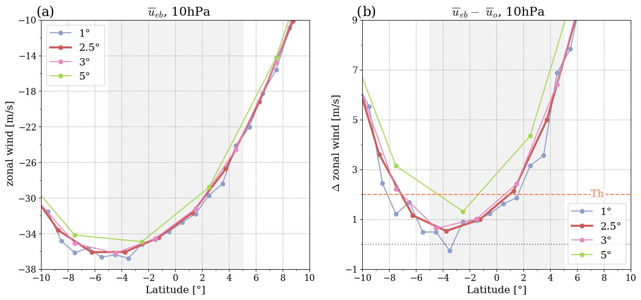
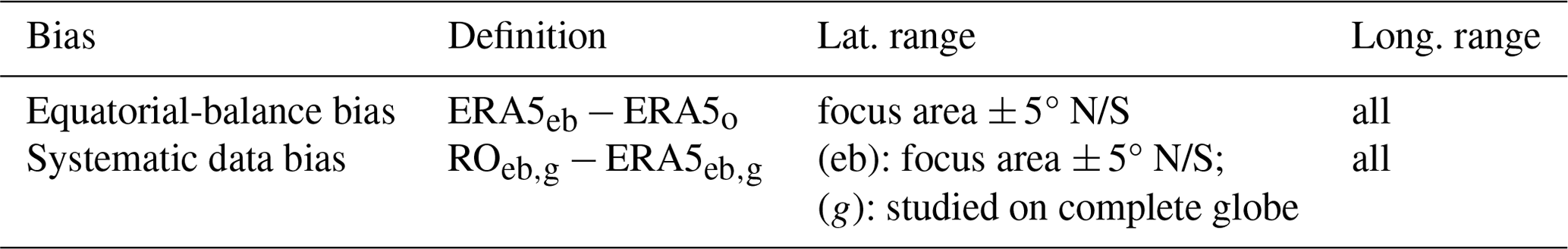
Figure 1Influence of different spatial resolutions on the zonal-mean wind component. Panel (a) shows the wind component, ueb; panel (b) the difference in the calculated wind to the ERA5 wind field zonal wind component, uo. The dashed orange line marks the 2 m s−1 threshold, and the results are shown for January 2009.
3.1 ERA5 reanalysis data
The ERA5 reanalysis data include global 3D wind information and geopotential height; it is therefore the ideal data set to test the validity of the equatorial-balance equation. It is available for a long time period and readily accessible via download from the Copernicus Climate Data Store (CCDS) (ECMWF-ERA5monthly, https://cds.climate.copernicus.eu/cdsapp#!/dataset/reanalysis-era5-pressure-levels-monthly-means?tab=overview, last access: 19 August 2024). The data are available on 37 levels from 1000 to 1 hPa, on a 0.25° × 0.25° grid. Different grid resolutions were investigated for wind derivation to find the sensible spatial grid for the equatorial-balance approximation. Figure 1 shows the result for the zonal equatorial-balanced wind, ueb, where Fig. 1a shows the result for the zonal wind component, tested for resolutions from 1 up to 5°, and Fig. 1b shows the difference to the original ERA5 zonal wind component, illustrated for January 2009.
The analysis in Fig. 1 illustrates that a grid spacing of 1° is counterproductive, as the u component shows large fluctuations. A grid of 2.5 or 3° results in similar values between derived and original wind fields. Furthermore, finer resolutions (temporal and spatial) increase the magnitude of the ageostrophic contributions, which are unbalanced (see Bonavita, 2023). On the other hand, for a 5° spacing, the loss in resolution is noticeable.
As a result, we chose a 2.5° × 2.5° climatology for all further ERA5 wind investigations. The data sets with lower resolutions were derived from the original 0.25° × 0.25° grid via cosine-weighted binning. The wind component data from the reanalysis is labeled uo, vo, and Vo, corresponding to the eastward, northward, and wind speed components. A line above the variable indicates a zonal average, e.g. . The wind components derived from the geopotential via the equatorial-balance equation are referred to as ueb, veb, and Veb or with a subscript g when we used the geostrophic approximation.
3.2 Radio-occultation data
In this study, we focus on the potential of RO data to derive monthly mesoscale (2.5° × 2.5°) wind products. A finer spatial resolution is, on the one hand, not recommended for RO data and this time period. This would require more dense global coverage with daily RO events, which is not available up to now (see also Angerer et al., 2017; Ladstädter et al., 2023). On the other hand, as a further physical reason, the geostrophic and equatorial balances will also not hold well at higher temporal or spatial resolutions, leading to larger ageostrophic contributions. We analyze the monthly RO climatology data from multi-satellite missions in the year 2009. The RO phase data were derived at UCAR/CDAAC (University Corporation for Atmospheric Research/COSMIC Data Analysis and Archive Center), while the further processing to geopotential height, Z(p), calculated on isobaric surfaces, p, was performed using the Wegener Center for Climate and Global Change (WEGC) Occultation Processing System OPSv5.6 (Angerer et al., 2017; Steiner et al., 2020). The WEGC OPSv5.6 retrieval system processes the atmospheric parameters as a function of altitude or geopotential height, based on the refractivity equation, the equation of state, and the downward integration of the hydrostatic equation. The physical atmospheric parameters (e.g., physical pressure) are derived using a moist-air retrieval algorithm, which combines the individual profiles with background information by optimal estimation; see Li et al. (2019) for details. The conversion to geopotential, Φ(p), is defined as , where g0 = ± 9.80665 m s−2, being the global standard gravity at mean sea level. In the year 2009, data are available from the following missions: Satèlite de Aplicaciones Científicas (SAC-C) (e.g., Hajj et al., 2004), Gravity Recovery And Climate Experiment (GRACE-A) (e.g., Beyerle et al., 2005), Formosa Satellite Mission 3/Constellation Observing System for Meteorology, Ionosphere, and Climate (Formosat-3/COSMIC) (e.g., Anthes et al., 2008), and from the Meteorological Operational Satellite (MetOp-A) (e.g., Luntama et al., 2008). The year 2009 was chosen as a representative data set to analyze the wind dynamics within a full year, having at the same time the advantage of rather high occultation statistics, due to the fully available six-satellite constellation of the Formosat-3/COSMIC mission (Angerer et al., 2017).
The monthly climatologies were produced on a 2.5° × 2.5° grid, using a 600 km radius which corresponds to the distance from the grid point, defined as the center location of the area of influence, within which the profiles contribute to the grid point mean. In performing the averaging, the profiles are weighted according to their distance from this center location with a bivariate (latitude–longitude) Gaussian function which peaks at the center and features a standard deviation of 150 km along latitude and 300 km along longitude, respectively. Details are given in the presentation by Ladstädter (2022). The geopotential climatologies, Φ(p), are available from 1000 to 5 hPa, on 147 levels. The geopotential was further binned to a 5° × 5° grid, using a cosine-weighted binning. From these larger bins, the equatorial-balanced winds were calculated. Tests revealed that a Gaussian smoothing with a 5° longitudinal smoothing window improved the wind data estimation, and the systematic difference decreased. This smoothing was therefore applied to the equatorial-balance wind fields derived from RO data. The larger binning was performed to avoid small fluctuations in the wind data, which required larger climatologies. Regarding geostrophic winds, the 2.5° × 2.5° grid could be maintained. The most prominent difference in the computation between equatorial and geostrophic winds is that the former requires a double derivative, while the latter requires a single derivative. Hence, small fluctuations in the data are enhanced for the equatorial-balance equation, which makes the derivation of winds a bigger challenge. However, we emphasize at this point that due to the COSMIC-2 mission (start in June 2019), which provides a higher sampling in the tropics, the potential of finer resolutions is given (Schreiner et al., 2020; Ho et al., 2020).
For the comparison between calculated ERA5 and RO wind, an interpolated ERA5 reanalysis data set with 364 levels from 1000 to 10 hPa was used. Since RO data were binned to a 5° × 5° grid (see Sect. 3.2 to have a sufficient number of observations per grid cell), the ERA5 data set was also transferred to a 5° × 5° grid, using cosine-weighted binning. For this specific data set, the prefix ERA is used.
To validate the equatorial-balance equation, the zonal and meridional wind components and wind speed were calculated according to the equations introduced in Eq. (2). We analyze the bias from the equatorial-balance equation in Sect. 4.1. The systematic bias between the observation-based RO data set and the reanalysis data set is investigated in Sect. 4.2. Hereby, the potential of RO wind products over the equatorial region is tested. The results on closing the gap across the Equator are discussed in Sect. 4.3. Furthermore, all vertically resolved plots are shown down to 800 hPa, since our focus is the free atmosphere, excluding the atmospheric boundary layer and hence frictional force.
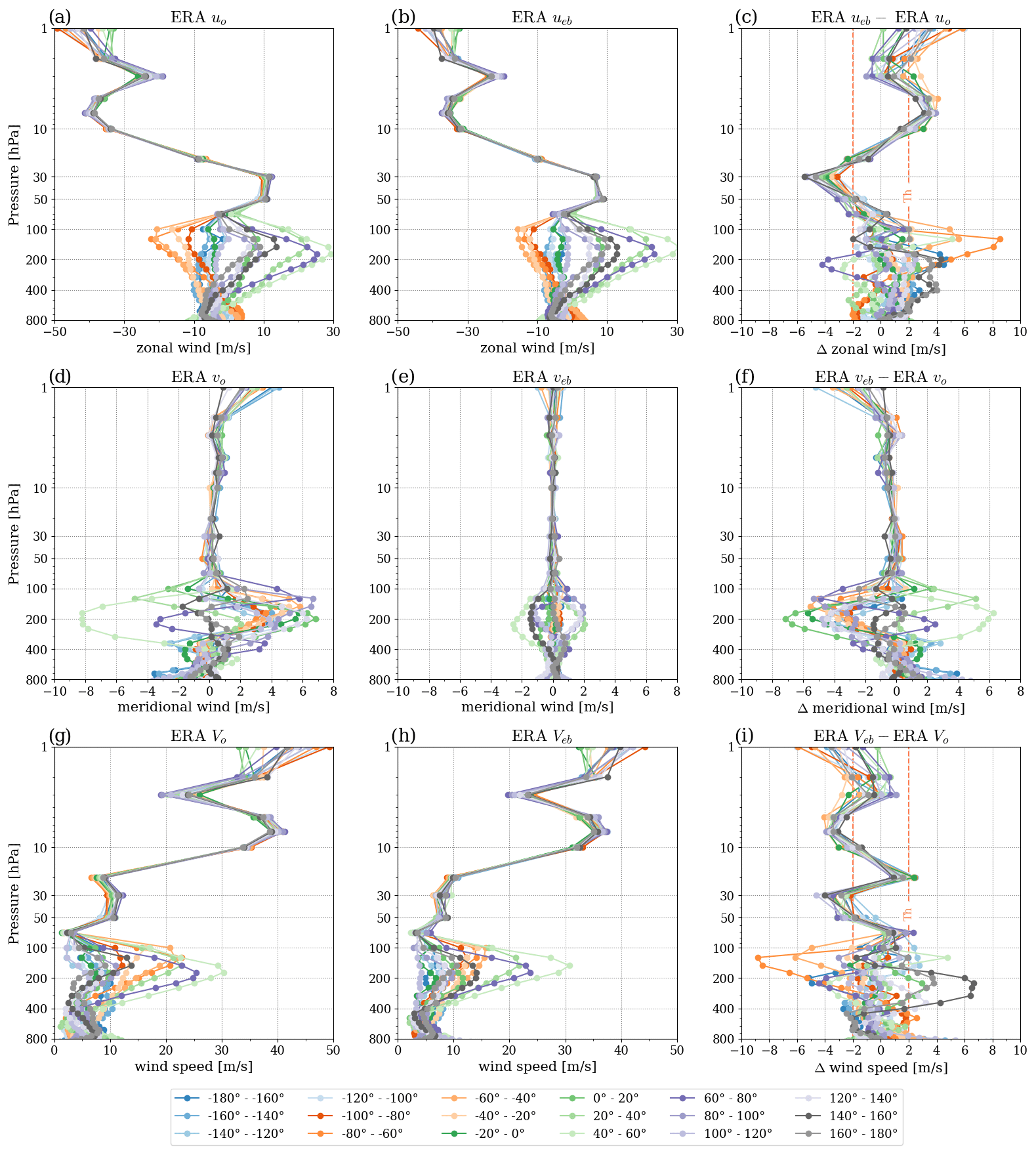
Figure 2Panels (a), (d), and (g) show the u, v, and V components of the original ERA5 data (a, d, and g). Panels (b), (e), and (h) show the wind components calculated with the equatorial-balance approximation. The last column (c, f, and i) illustrates the difference between the derived and original wind data from ERA5. The wind components and wind speed are studied for 20° meridional bands and a ± 5° latitudinal averaging. The data are from January 2009.
4.1 ERA5 wind validation
To test the quality of the equatorial-balance equation, both wind components individually and the total wind speed are compared to the original wind field in ERA5. Figure 2 shows the original wind with the wind component and wind speed calculated with the equatorial-balance equation, as well as the respective differences for January 2009. The analysis was performed in 20° meridional bands. We find that the zonal wind component shows maximum magnitudes larger than −30 m s−1 around 8 hPa and up to 10 m s−1 between 50 to 30 hPa for both original and derived zonal winds (Fig. 2a and b).
The analysis of the difference between computed and original ERA5 fields generally illustrates a good agreement within ± 2 m s−1 in the stratosphere, reaching ± 5 m s−1 when the absolute magnitudes reach maximum values, i.e., around 8 hPa and between 50 to 30 hPa, respectively. Furthermore, the analysis shows that the different longitude bands coincide in the stratosphere. Also, in the middle to upper troposphere, the difference between the derived winds and the original winds is predominantly within the threshold; however, the individual longitude bands do not coincide anymore (pressures higher than the 100 hPa level).
In Fig. 2d–f, we show the meridional wind component, where the magnitudes of the wind speed are much smaller. We show here the results of the meridional wind component for all longitude bands. In further analysis, we will only present results based on one exemplary longitude band around the prime (Greenwich) meridian (−10 to 10° longitude), keeping notice that we had studied the other sectors as well, which qualitatively showed similar behavior. First of all, the meridional wind is very small in the tropical stratosphere (see Fig. 2d and e). Second, the meridional wind is much smaller than the zonal wind (close to zero compared to the zonal wind). Third, even the bias in the zonal component is larger than the meridional component itself, and finally, since the meridional wind is very small, it cannot be well represented by the equatorial-balance equation. In the troposphere, the meridional wind speed increases to values around ± 4 m s−1. Analyzing the equatorial-balance bias shows that the difference fluctuates with amplitudes of about ± 2 to 4 m s−1 in the tropical troposphere (Fig. 2f).
Finally, we study the total wind speed (Veb, Fig. 2g–i). To this end, the question is if the meridional wind component has an added value for the total wind speed (), since its magnitude is close to zero in the stratosphere. In this first analysis, we included the meridional wind component in the computation of wind speed, finding that it was possible to derive the wind fields close to the original wind speed (Fig. 2g and h), and within our defined threshold (Fig. 2h), from the middle troposphere up to the stratosphere.
Figure 3Absolute (a, b) and relative difference (c, d) between derived and original ERA5 zonal-mean total wind speed, shown as vertical–latitudinal cross sections. The first column (a, c) uses only the zonal-mean component as an approximation for wind speed, while the second column (b, d) includes the zonal and meridional component to estimate the total wind speed. The data are from January 2009.
To better understand the potential added value of the meridional wind component in total wind speed, we study in Fig. 3 the impact of the v component on the final product in more detail. We show a vertical–latitudinal cross section and approximate the zonal-mean wind speed by only using the zonal wind component (Fig. 3a and b), compared to including both components for the zonal-mean wind speed estimate (Fig. 3b and d). We study the absolute (Fig. 3a and b) and relative (Fig. 3c and d) differences to the original ERA5 data. In the absolute difference, the two estimates of zonal-mean wind speed show very similar results in the stratosphere. This is because the meridional component is close to zero in magnitude, having only a negligible impact on the total wind speed.
The situation changes in the troposphere at pressures higher than the 100 hPa level. The zonal-mean wind speed clearly improves when including the meridional wind component for the estimate of wind speed (compare Fig. 3a and b). The differences between derived and calculated wind speed are mainly within the target threshold of ± 2 m s−1 when including the meridional wind. Also, the relative difference (Fig. 3c and d) illustrates this clear improvement in the zonal-mean wind speed data, when comparing Fig. 3c and d. This result indicates that while the meridional component itself is not well estimated, the calculation of the zonal-mean total wind speed shows a somewhat closer agreement from also including this small wind component in the troposphere. That is, the slight underestimation left by the zonal wind speed in the troposphere (see Fig. 3a and c) is mitigated by the inclusion of the meridional wind speed, which brings the approximated zonal-mean total wind speed closer to the original one (see Fig. 3b and d). The reason for this small co-benefit to the zonal-mean total wind speed is that the averaged meridional wind speed is estimated by the balance approximation at about the right (small) magnitude in the troposphere. However, in the stratosphere, the close-to-zero meridional wind brings in no further improvement. Nevertheless, we caution that, in addition to finding the meridional wind estimates not viable to benefit also longitude-resolved wind speeds, we also find them not viable to reconstruct wind direction (i.e., wind vectors on top of wind speed estimates). The reason is that the direction of the approximated meridional wind at individual grid points is nearly as often found opposite as it is found aligned with the original wind direction.
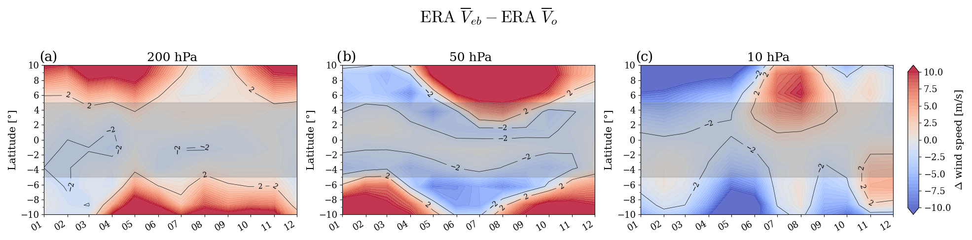
Figure 4Seasonal development of the zonal-mean total wind speed bias resulting from the equatorial-balance equation for the year 2009, studied for ERA5 data at three representative pressure levels.
Furthermore, we investigate the bias resulting from the equatorial-balance approximation for the complete year 2009 (Fig. 4). We show these results on the three representative levels (200, 50, and 10 hPa), representing the tropical upper troposphere, lower stratosphere, and middle stratosphere, respectively. Across all seasons, the equatorial-balance approximation shows best results in the absolute difference at lower altitudes. For the lower stratosphere, the region below the bias threshold shifts away from the Equator with the seasons, with an offset in the direction of the winter hemisphere. For 10 hPa, the middle stratosphere, the approximation is least accurate during Northern Hemisphere summer months.
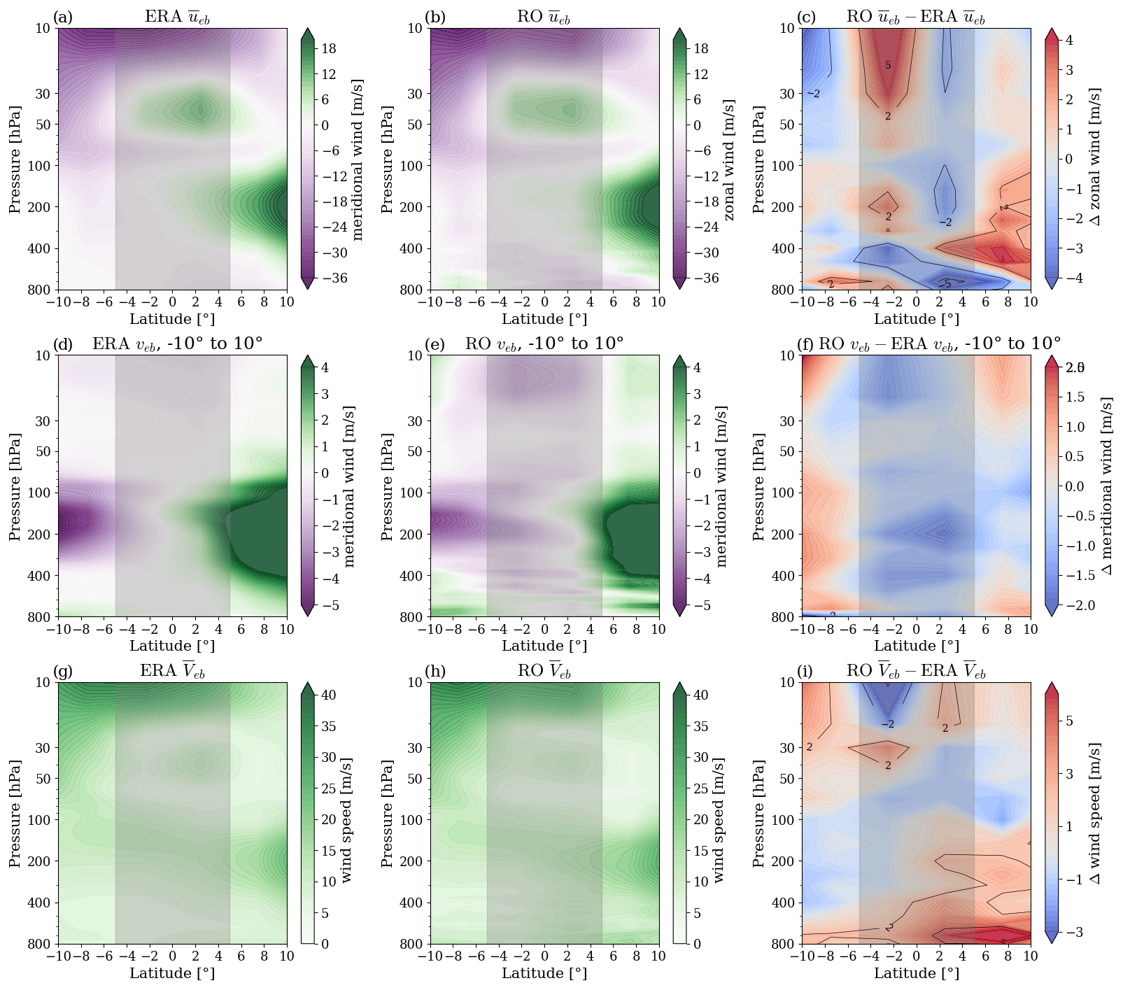
Figure 5Panels (a), (d), and (g) show the u, v, and V components calculated with the equatorial-balance approximation for ERA5 data, while panels (b), (e), and (h) show the same using RO data. The last column (c, f, and i) illustrates the difference between the values calculated between RO data and ERA5 data. Note that u and V are plotted as a zonal average, while the v component is shown as an example for the longitude sector of −10 to 10°. The data are from January 2009.
4.2 RO wind validation
In this section, we investigate the systematic data bias between RO and ERA5-derived wind fields. To remind the reader, we use a two-step approach to assess the potential of using the equatorial-balance equation for RO wind field derivation across the Equator (see also Table 1). In a first step, we decomposed the analysis into the bias originating from the approximation itself (first step, only ERA5, Sect. 4.1). In a second step, we then assess the systematic bias between the two data sets (ERA5 and RO) to understand where differences between them occur. First of all, we observe that for RO ueb, RO veb, and RO Veb the spatial patterns look very similar to the wind fields calculated with ERA5 data (see Fig. 5). Between 30 and 10 hPa, the bias between the two data sets and for the zonal wind (ueb, Fig. 5a–c) lies between ± 2 m s−1 and ± 5 m s−1, increasing towards higher altitudes (Fig. 5c). A possible reason could be that the impact of the residual ionospheric error, as well as measurement noise, increase towards higher altitudes for RO data (e.g., Danzer et al., 2013, 2018; Liu et al., 2020, 2024). With the exception of this region and the boundary layer, the target threshold of ± 2 m s−1 is rarely exceeded, and the wind speed differences are very small between the two data sets. When considering the differences between the two data sets for meridional wind and wind speed (Fig. 5f and i), it is seen that these also generally reside within ± 2 m s−1. Nevertheless, due to the already small absolute magnitudes of the meridional wind (Fig. 5d and e), it is also clear that this component itself is not well reproduced. However, the zonal-mean total wind speed (Fig. 5g–i) still shows an improvement in the troposphere from including both wind components (Fig. 5i), with the dominant contribution coming from the zonal component.
Nimac et al. (2023) found that the bias between RO Vg and ERA Vg decreased after 2016, when ERA5 undertook a major observing system change. It is reasonable to assume that a similar behavior could be observed for RO Veb and ERA Veb. As the number of RO satellite missions in operation changes, there are fluctuations in the number of available RO profiles to aggregate for a given time period. The years 2008 and 2009 show a high number of daily occultations (roughly 2500 to 3000 events). In the years 2011 and 2012, there is a significant drop in the daily available occultations (roughly 1500 events) (see Angerer et al., 2017). In those years, we have no further data from one of the six Formosat-3/COSMIC (F3C) satellites; also, the SAC-C mission ended. However, with the launch of the COSMIC-2 mission in 2019, which is specifically designed for a high coverage in the tropics up to the midlatitudes (Schreiner et al., 2020; Ho et al., 2020), the accuracy of RO data in the equatorial region will further increase. This possibly also allows researchers to use a 2.5° × 2.5° wind field grid in future studies.
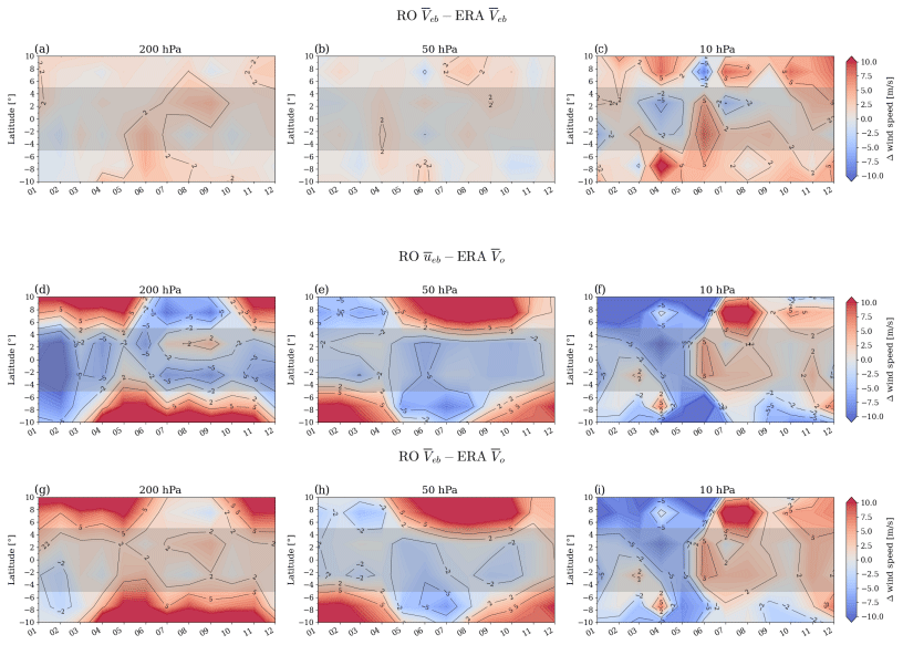
Figure 6Seasonal development of the systematic data bias (a–c) between RO and ERA5 data, studied for the year 2009 on three representative pressure levels. Second (d–f) and third (g–i) rows illustrate the seasonal development of the zonal-mean total wind speed bias, using for the former only the zonal component as an approximation for wind speed, while the latter includes the zonal and meridional components in the estimate.
In a final analysis, we investigated the seasonal development of the systematic (first row) and total wind speed bias (second and third rows) for the complete year 2009 (see Fig. 6). With respect to the systematic data bias (first row) between RO (RO Veb) and ERA5 (ERA Veb), there is little to no deviation from the upper troposphere (200 hPa) to the lower stratosphere (50 hPa) all year. Only at the 10 hPa level do we observe somewhat larger deviations, most notable in the Northern Hemisphere summer months. The numbers of RO profiles accumulated to generate the monthly RO data set dropped by around 33 % in June 2009 compared to other months in the same year. This possibly decreases the data quality; therefore, we observe an increase in the systematic data bias (e.g., Scherllin-Pirscher et al., 2011; Schwarz et al., 2017). The bias is within ± 2 and ± 5 m s−1, indicating that towards high altitudes the wind speed retrieval over the tropics becomes more challenging. We still see potential for improvements in the ongoing work by correcting residual biases of RO data in the upper stratosphere (Danzer et al., 2021; Liu et al., 2020).
The second and third rows of Fig. 6 examine the difference between RO-computed winds relative to the original ERA5 winds. The second row only uses the zonal wind component for the estimate of the zonal-mean total wind speed, while in the third row both the zonal and meridional components are included. When comparing the two rows, the results illustrate an improvement for zonal-mean wind speed when including the meridional wind (third row). The geographical band we are focusing on is between ± 5° latitude (light shaded grey area). Within this area, the bias clearly decreases between RO and ERA5 wind speed, at the 200 and 50 hPa levels. At the 10 hPa level, the pattern is similar between the second and third rows, illustrating the decreasing influence of the meridional wind component; see also the discussion in Sect. 4.1.
Summarizing the results of the current and previous section, the climate wind field derivation was possible across the Equator using RO data when focusing on its core vertical region of high quality and resolution. Furthermore, we found that although the meridional component itself is not well estimated it is the zonal-mean total wind speed in the troposphere that shows a closer agreement with the corresponding original wind speed when including both components, while in the stratosphere the meridional component's influence becomes negligible.
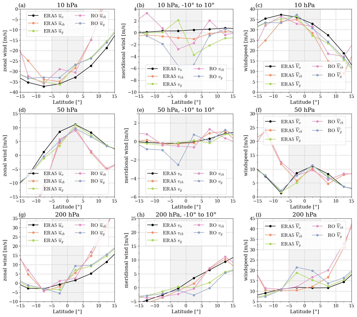
Figure 7Detailed analysis of zonal wind (u; a, d, and g), meridional wind (v; b, e, and h), and wind speed (V; c, f, and i), at the three pressure levels of 10, 50, and 200 hPa (first to third rows). Results are shown for the original (o), equatorial-balanced (eb), and geostrophic (g) ERA5 data and RO data (eb, g). u and V are plotted as the zonal mean, while the v component is calculated as a mean from the longitudinal sector −10 to 10°. The data are from January 2009.
4.3 Closing the equatorial gap
In this final results section, we aim to bridge the wind field gap over the Equator to end up with a wind field product over the complete globe. For this reason, we have once more taken a closer look at the zonal and meridional winds, as well as wind speed, at the three respective pressure levels of 10, 50, and 200 hPa (Fig. 7a–c and g–i). In Fig. 7, we compare the computed winds, i.e., equatorial-balance (eb) and geostrophic-balance (g) RO and ERA5 winds, to original (o) ERA5 winds (solid black line). We analyze how the equatorial-balance and geostrophic-balance approximations bridge over the Equator, thereby finding some interesting results. We observe that the zonal geostrophic wind () actually does not break down between ± 5°, neither for RO-computed nor ERA5-computed winds. The results for are actually closer to the original wind (black line, Fig. 7a, d, and g) than the computed zonal equatorial-balanced winds (ueb, RO and ERA5). The component primarily responsible for the increase in the geostrophic bias over the Equator is the meridional wind component (vg), showing the largest differences with respect to the original ERA5 meridional component (vo) at 10 hPa, decreasing towards 200 hPa (Fig. 7b, e, and h). Here, the equatorial-balance solution (veb, RO and ERA5) clearly better reproduces the ERA5 meridional winds, having the smallest bias at 200 hPa, with an increasing bias towards 10 hPa. Since the geostrophic meridional wind drives the equatorial breakdown (vg), as a result the geostrophic wind speed (Vg) also shows larger biases over the Equator, while the equatorial wind speed (Veb) is a better fit between ± 5° (Fig. 7c, f, and i).
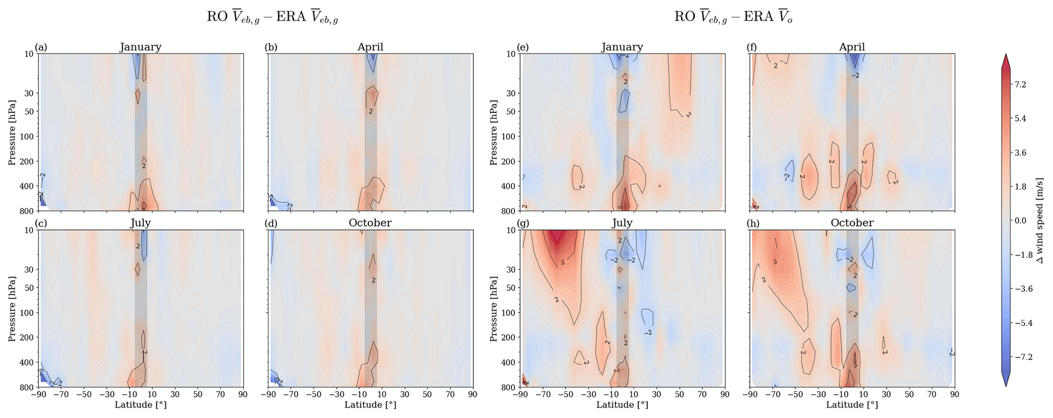
Figure 8Zonal-mean systematic data bias, panels (a) to (d), and zonal-mean wind speed bias, panels (e) to (h). To construct the RO and ERA wind fields, the equatorial-balance equation is used inside the equatorial band (|Lat.| < 5, while outside this region the geostrophic-balance approximation is used. The data are from January 2009.
Finally, we use our knowledge from the prior analysis to compute a complete global wind field data set, using RO data. In Fig. 8, we show the result based on the four seasonal representative months: January, April, July, and October. The wind fields are illustrated as a vertical cross section from 800 to 10 hPa, depending on latitude. The left-hand side of this plot (Fig. 8a–d) shows the bias between the computed RO wind fields relative to ERA5-computed wind fields. Between ± 5°, we use the equatorial-balance equation for the calculation of the wind speed (Veb), while outside this latitude band the geostrophic-balance approximation is applied (Vg). We find that the bias between the two data sets is very low, with differences dominantly less than ± 2 m s−1. In the equatorial latitude band, we find small exceedances in the lower troposphere, while the upper troposphere and lower stratosphere (UTLS) are very close to ERA5. This feature clearly relates to the core region of high-quality RO data, which is in the upper troposphere and lower stratosphere. With decreasing altitude and therefore increasing moisture content, the retrieval of atmospheric parameters relies increasingly on background information (e.g., Li et al., 2019). The RO information dominates between about 8 to 35 km in the tropics (e.g., Scherllin-Pirscher et al., 2011).
As a final comparison, we show on the right-hand side (Fig. 8e–h) the respective RO wind fields relative to the original ERA5 wind data. We can conclude that the quality of the wind fields is, especially above 500 hPa, very good and mostly within the target of ± 2 m s−1. Outside this latitude band, we apply the geostrophic approximation, and we also find a high wind speed quality. Exceptions are the stratospheric polar jet stream and the subtropical jet stream, where larger deviations are found. However, this was not part of this specific analysis. More information can be found in Nimac et al. (2023, 2024).
In this study, we investigated the potential of radio-occultation (RO) data for climate-oriented wind field monitoring in the tropics, with a specific focus on the equatorial band within ± 5° latitude. We analyzed the equatorial-balance equation within this band and computed RO wind fields at a 5° × 5° resolution. In a wider range over the tropics, we computed the RO wind fields, using the geostrophic approximation, on a higher-resolved 2.5° × 2.5° grid. We also calculated the winds using ERA5 data, applying the same physical equations and resolutions for the comparison analysis (basic ERA5 resolution 2.5° × 2.5°).
In a first step, we analyzed the bias solely resulting from the equatorial-balance approximation by studying the difference between computed winds from ERA5 geopotential and original ERA5 winds. In a second step, we compared the balance-derived approximate RO winds to the approximative ERA5 winds. This two-step approach allowed us to separately study the bias resulting from the approximation itself and the systematic bias between the two data sets. We also analyzed how the geostrophic and equatorial-balanced zonal winds, meridional winds, and wind speeds bridge across the Equator to understand which wind component drives the geostrophic breakdown over the Equator.
The results showed that we could successfully apply the equatorial-balance equation for the RO wind field computation across the Equator. For the u component this was already examined by Healy et al. (2020) in a zonal analysis. In our study, we were able to resolve the zonal wind by a 5° × 5°, latitude × longitude, grid. Furthermore, we included in this analysis the meridional wind component, as well as total wind speed, applying the same grid resolution. However, the meridional wind component was challenging, since its wind speed is in general an order of magnitude smaller than the zonal wind in the troposphere, while in the stratosphere its contribution is negligible. Hence, a wind flow with small magnitudes and changes in the direction of the flow (changing sign) is challenging to reproduce. We find, in this respect, that the equatorial-balance approximation is not suitable for the reconstruction of wind directions or longitude-resolved wind speeds in the troposphere.
Nevertheless, the analysis clearly showed that calculating both the zonal and meridional wind components resulted in a higher quality of the zonal-mean total wind speed in the troposphere. In the stratosphere, total wind speed is governed by the zonal component, and there is no added value furnished by the meridional component. In general, the equatorial-balance approximation works best in the stratosphere. The biases were mostly within the target requirement of ± 2 m s−1, decreasing a bit in quality upward towards the 10 hPa level. In this respect, we emphasize that the COSMIC-2 mission (Schreiner et al., 2020; Ho et al., 2020), with dense RO event coverage in the tropics, will substantially improve RO wind fields in this area. Furthermore, the potential exists in this case to refine to the desirable 2.5° × 2.5° resolution for the wind field data.
Another important result was found when analyzing the individual wind components (u and v) and total wind speed (V) for geostrophic (g), equatorial-balanced (eb), and original (o) winds, comparing RO and ERA5 data. We found that the dominant wind component, which drives the geostrophic breakdown, is the meridional wind, while the zonal geostrophic wind also works well across the Equator. The geostrophic zonal wind (ug) performed even a bit better in quality than the equatorial zonal wind (ueb). Nevertheless, the equatorial-balance approximation works as a robust solution of the wind equation just within the equatorial ± 5° band. Outside this band, it is no longer a valid approximation and hence breaks down. We also tested combinations of the total wind speed in this region, as a vector sum of zonal geostrophic wind and meridional equatorial wind in a specific altitude range. The results were quite satisfactory as well (not shown), but exploring in detail a most suitable combined wind field construction needs to be part of a future study.
To summarize, we found encouraging results in that we revealed that RO data do indeed have good potential for long-term wind field monitoring over the complete globe, including across the Equator. A regional-scale climate resolution (5° × 5°, latitude × longitude, grid) was possible to demonstrate for the RO data in this specific region for wind speed, with evidence for added value from their accuracy and high resolution, as well as their long-term stability.
We tested different finite-differencing techniques (centered, forward, backward, and centralized with higher-order). We found that while forward and backward differencing is not recommended (for truncation errors being of order 𝒪(h)), centralized and higher-order centralized methods show very similar results when using ERA5 data on a 2.5° × 2.5° grid.
The standard central (Eq. A1) and higher-order central (Eq. A2) finite difference methods for the second-derivative (curvature) operator , on a function f(x), with h being the step size of the numerical grid, were used in our study through the following conventional formulations:
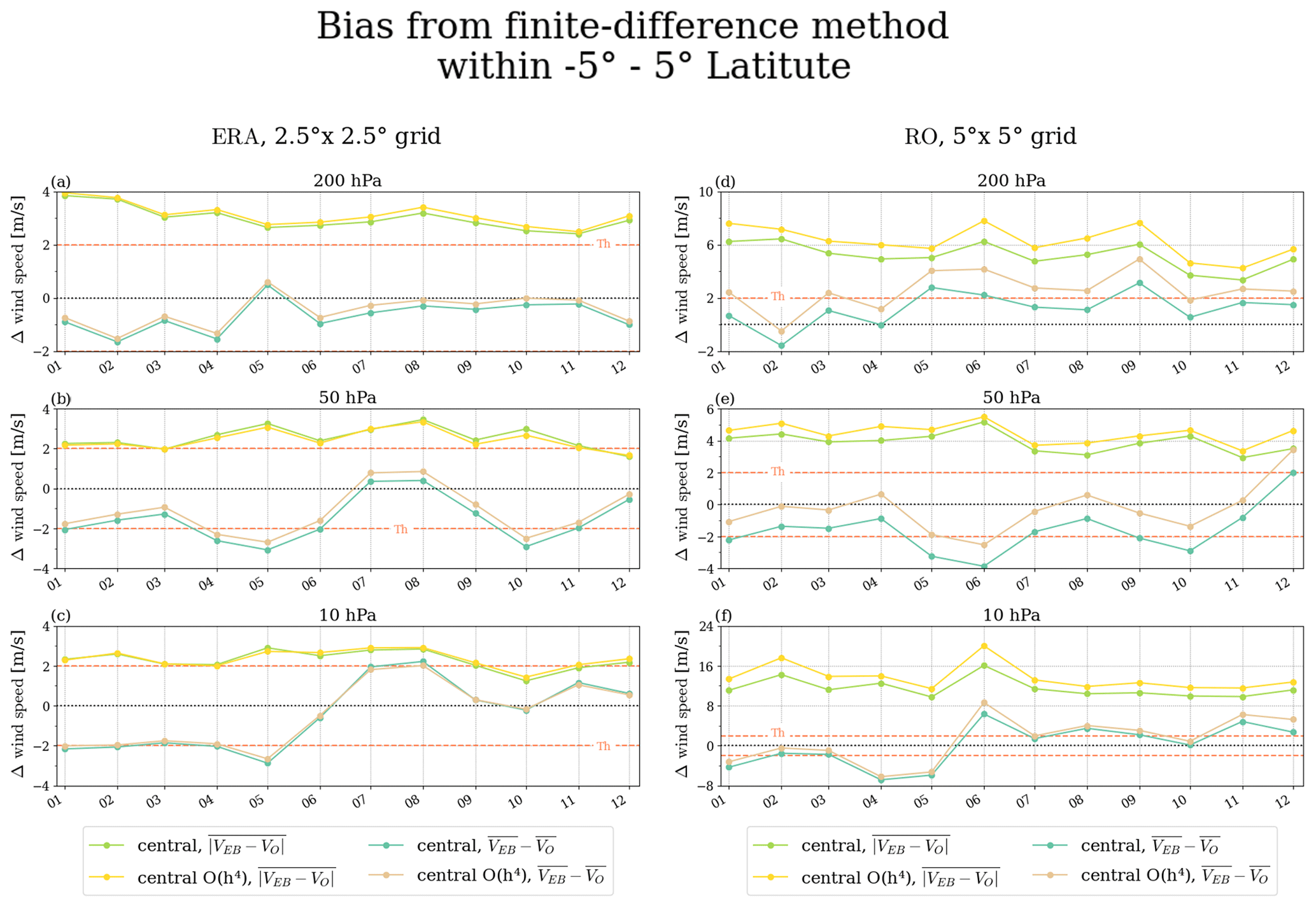
Figure A1Figure illustrating the bias resulting from using two different finite difference methods, i.e., comparing standard centralized and higher-order centralized differencing. To show different relevant aspects of averaging, the bias is computed as the zonal-mean bias between balance-derived RO or ERA5 wind field and original ERA5 wind field (), as well as the local bias within individual grid cells, taking afterwards the zonal mean (). Panels (a), (b), and (c) show the bias for ERA5 data, while panels (d), (e), and (f) show the bias for RO data.
Figure A1 illustrates the bias differences that result between these two finite-difference methods. The left column shows the bias based on ERA5 data (balance-derived versus original), while the right column shows the impact of the bias based on RO data (balance-derived versus original). We inspect the two relevant bias types: (i) a zonal mean () between derived wind field and original ERA5 wind and (ii) the local bias within single grid cells, taking the zonal mean afterwards ().
We find for the ERA5 data (left column), computed on a 2.5° × 2.5° grid, that the local approximation bias at individual grid points () is slightly smaller when using the standard central method, while the zonal-mean bias improves a bit with the higher-order method. These biases are amplified when using the RO data available on a 5° × 5° grid (right column). Here the difference in the local bias is found to be larger, with the standard central method outperforming the higher-order method. This larger local bias of the higher-order five-point method (Eq. A2) compared to the standard three-point method (Eq. A1) is likely caused by the fairly large latitudinal range of the former across the central grid point, spanning across four 5° steps.
For the zonal-mean bias, again the higher-order method performs somewhat better, with the quality depending on altitude level and month. Overall, since the equatorial-balance approximation is, strictly speaking, only fully valid at the Equator, the approximation error from including data points outside of the ± 5° Equator band is considered larger than the gain from applying the higher-order method. For this reason, the standard centered differencing method was finally chosen as the primary method for the respective data analyses in this study.
All computed wind field data for the year 2009 can be found under WEGC Cloud (last access: 19 August 2024). The folder contains the following three files: (i) the wind fields calculated from the WEGC Occultation Processing System OPSv5.6 RO data, (ii) the wind fields calculated from ERA5 reanalysis data and further interpolated at the WEGC, and (iii) the wind fields calculated from the download from the Copernicus Climate Data Store. The original RO OPSv5.6 data are available under https://doi.org/10.25364/WEGC/OPS5.6:2021.1 (WEGC, 2024).
Conceptualization: JD, GK; Data curation: MP; Formal analysis: MP, JD; Funding acquisition: JD; Methodology: JD, GK; Supervision: JD, GK; Validation and visualization: MP, JD, GK; Writing (original draft preparation): JD, MP; Writing (review and editing): JD, GK.
The contact author has declared that none of the authors has any competing interests.
Publisher's note: Copernicus Publications remains neutral with regard to jurisdictional claims made in the text, published maps, institutional affiliations, or any other geographical representation in this paper. While Copernicus Publications makes every effort to include appropriate place names, the final responsibility lies with the authors.
This article is part of the special issue “Observing atmosphere and climate with occultation techniques – results from the OPAC-IROWG 2022 workshop”. It is a result of the International Workshop on Occultations for Probing Atmosphere and Climate, Leibnitz, Austria, 8–14 September 2022.
We thank the UCAR/CDAAC RO team for providing RO excess phase and orbit data and the WEGC RO team for providing the OPSv5.6 retrieved profile data. We particularly thank Florian Ladstädter (WEGC) for providing the monthly gridded climatology data and Irena Nimac for supplying the initial scripts, from which the wind field derivations were further developed. Furthermore, we thank the ECMWF for providing access to the ERA5 reanalysis data. We are also grateful for fruitful discussions with Albert Osso (WEGC). Finally, we thank the Austrian Science Fund (FWF) for funding the work; the wind analysis is part of the FWF stand-alone project Strato-Clim (grant no. P-40182).
This research has been supported by the Austrian Science Fund (grant no. P-40182).
This paper was edited by Kent B. Lauritsen and reviewed by two anonymous referees.
Angerer, B., Ladstädter, F., Scherllin-Pirscher, B., Schwärz, M., Steiner, A. K., Foelsche, U., and Kirchengast, G.: Quality aspects of the Wegener Center multi-satellite GPS radio occultation record OPSv5.6, Atmos. Meas. Tech., 10, 4845–4863, https://doi.org/10.5194/amt-10-4845-2017, 2017. a, b, c, d, e, f
Anthes, R. A.: Exploring Earth's atmosphere with radio occultation: contributions to weather, climate and space weather, Atmos. Meas. Tech., 4, 1077–1103, https://doi.org/10.5194/amt-4-1077-2011, 2011. a
Anthes, R. A., Bernhardt, P. A., Chen, Y., Cucurull, L., Dymond, K. F., Ector, D., Healy, S. B., Ho, S.-P., Hunt, D. C., Kuo, Y.-H., Liu, H., Manning, K., McCormick, C., Meehan, T. K., Randel, W. J., Rocken, C., Schreiner, W. S., Sokolovskiy, S. V., Syndergaard, S., Thompson, D. C., Trenberth, K. E., Wee, T.-K., Yen, N. L., and Zeng, Z.: The COSMIC/FORMOSAT-3 mission: Early results, B. Am. Meteorol. Soc., 89, 313–333, https://doi.org/10.1175/BAMS-89-3-313, 2008. a, b
Baker, W. E., Atlas, R., Cardinali, C., Clement, A., Emmitt, G. D., 60 Gentry, B. M., Hardesty, R. M., Källén, E., Kavaya, M. J., Langland, R., Ma, Z., Masutani, M., McCarty, W., Pierce, R. B., Pu, Z., Riishojgaard, L. P., Ryan, J., Tucker, S., Weissmann, M., and Yoe, J. G.: Lidar-measured wind profiles, B. Am. Meteorol. Soc., 95, 543–564, https://doi.org/10.1175/BAMS-D-12-00164.1, 2014. a
Beyerle, G., Schmidt, T., Michalak, G., Heise, S., Wickert, J., and Reigber, C.: GPS radio occultation with GRACE: Atmospheric profiling utilizing the zero difference technique, Geophys. Res. Lett., 32, L13806, https://doi.org/10.1029/2005GL023109, 2005. a
Bodeker, G., Bojinski, S., Cimini, D., Dirksen, R., Haeffelin, M., Hannigan, J., Hurst, D., Leblanc, T., Madonna, F., Maturilli, M., A. C. Mikalsen, Philipona, R., Reale, T., Seidel, D. J., Tan, D. G. H., Thorne, P. W., Vömel, H., and Wang, J.: Reference upper-air observations for climate: From concept to reality, B. Am. Meteorol. Soc., 97, 123–135, 2016. a
Bonavita, M.: On the limitations of data-driven weather forecasting models, arXiv [preprint], arXiv:2309.08473, 2023. a
Cardinali, C. and Healy, S.: Impact of GPS radio occultation measurements in the ECMWF system using adjoint-based diagnostics, Q. J. Roy. Meteor. Soc., 140, 2315–2320, https://doi.org/10.1002/qj.2300, 2014. a
Chandra, S., Fleming, E. L., Schoeberl, M. R., and Barnett, J. J.: Monthly mean global climatology of temperature, wind, geopotential height and pressure for 0–120 km, Adv. Space Res., 10, 3–12, https://doi.org/10.1016/0273-1177(90)90230-W, 1990. a, b
Cucurull, L.: Improvement in the use of an operational constellation of GPS radio occultation receivers in weather forecasting, Weather Forecast., 25, 749–767, 2010. a
Danzer, J., Scherllin-Pirscher, B., and Foelsche, U.: Systematic residual ionospheric errors in radio occultation data and a potential way to minimize them, Atmos. Meas. Tech., 6, 2169–2179, https://doi.org/10.5194/amt-6-2169-2013, 2013. a
Danzer, J., Schwärz, M., Proschek, V., Foelsche, U., and Gleisner, H.: Comparison study of COSMIC RO dry-air climatologies based on average profile inversion, Atmos. Meas. Tech., 11, 4867–4882, https://doi.org/10.5194/amt-11-4867-2018, 2018. a
Danzer, J., Haas, S. J., Schwaerz, M., and Kirchengast, G.: Performance of the ionospheric Kappa correction of radio occultation profiles under diverse ionization and solar activity conditions, Earth Space Sci., 8, e2020EA001581, https://doi.org/10.1029/2020EA001581, 2021. a
English, S., McNally, T., Bormann, N., Salonen, K., Matricardi, M., Moranyi, A., Rennie, M., Janisková, M., Di Michele, S., Geer, A., Tomaso, E., Cardinali, C., de Rosnay, P., Sabater, J. M., Bonavita, M., Albergel, C., Engelen, R., and Thépaut, J.-N.: Impact of satellite data, ECMWF Technical Memoranda, October 2013, 2013. a
Eyre, J. R., English, S. J., and Forsythe, M.: Assimilation of satellite data in numerical weather prediction. Part I: The early years, Q. J. Roy. Meteor. Soc., 146, 49–68, 2020. a
Foelsche, U., Pirscher, B., Borsche, M., Kirchengast, G., and Wickert, J.: Assessing the climate monitoring utility of radio occultation data: From CHAMP to FORMOSAT-3/COSMIC, Terr. Atmos. Ocean. Sci., 20, 155–170, https://doi.org/10.3319/TAO.2008.01.14.01(F3C), 2009. a
Foelsche, U., Scherllin-Pirscher, B., Ladstädter, F., Steiner, A. K., and Kirchengast, G.: Refractivity and temperature climate records from multiple radio occultation satellites consistent within 0.05 %, Atmos. Meas. Tech., 4, 2007–2018, https://doi.org/10.5194/amt-4-2007-2011, 2011a. a
Foelsche, U., Syndergaard, S., Fritzer, J., and Kirchengast, G.: Errors in GNSS radio occultation data: relevance of the measurement geometry and obliquity of profiles, Atmos. Meas. Tech., 4, 189–199, https://doi.org/10.5194/amt-4-189-2011, 2011b. a
Geer, A. J., Lonitz, K., Weston, P., Kazumori, M., Okamoto, K., Zhu, Y., Liu, E. H., Collard, A., Bell, W., Migliorini, S., Chambon, P., Fourrié, N., Kim, M.-J., Köpken-Watts, C., and Schraff, C.: All-sky satellite data assimilation at operational weather forecasting centres, Q. J. Roy. Meteor. Soc., 144, 1191–1217, 2018. a
Hajj, G. A., Kursinski, E. R., Romans, L. J., Bertiger, W. I., and Leroy, S. S.: A technical description of atmospheric sounding by GPS occultation, J. Atmos. Sol.-Terr. Phy., 64, 451–469, https://doi.org/10.1016/S1364-6826(01)00114-6, 2002. a
Hajj, G. A., Ao, C., Iijima, B., Kuang, D., Kursinski, E., Mannucci, A., Meehan, T., Romans, L., de La Torre Juarez, M., and Yunck, T.: CHAMP and SAC-C atmospheric occultation results and intercomparisons, J. Geophys. Res.-Atmos., 109, D6, https://doi.org/10.1029/2003JD003909, 2004. a
Healy, S.: Operational assimilation of GPS radio occultation measurements at ECMWF, ECMWF Newsletter, 111, 6–11, 2007. a
Healy, S. B., Polichtchouk, I., and Horányi, A.: Monthly and zonally averaged zonal wind information in the equatorial stratosphere provided by GNSS radio occultation, Q. J. Roy. Meteor. Soc., 146, 3612–3621, https://doi.org/10.1002/qj.3870, 2020. a, b, c
Hersbach, H., Bell, B., Berrisford, P., Hirahara, S., Horányi, A., Muñoz-Sabater, J., Nicolas, J., Peubey, C., Radu, R., Schepers, D., Simmons, A., Soci, C., Abdalla, S., Abellan, X., Balsamo, G., Bechtold, Biavati, P., G., Bidlot, J., Bonavita, M., De Chiara, G., Dahlgren, P., Dee, D., Diamantakis, M., Dragani, R., Flemming, J., Forbes, R., Fuentes, M., Geer, A., Haimberger, L., Healy, S., Hogan, R. J., Hólm, E., Janisková, M., Keeley, S., Laloyaux, P., Lopez, P., Lupu, C., Radnoti, G., de Rosnay, P., Rozum, I., Vamborg, F., Villaume, S., and Thépaut, J.-N.: The ERA5 global reanalysis, Q. J. Roy. Meteor. Soc., 146, 1999–2049, 2020. a, b, c
Ho, S.-P., Zhou, X., Shao, X., Zhang, B., Adhikari, L., Kireev, S., He, Y., Yoe, J. G., Xia-Serafino, W., and Lynch, E.: Initial assessment of the COSMIC-2/FORMOSAT-7 neutral atmosphere data quality in NESDIS/STAR using in situ and satellite data, Remote Sens., 12, 4099, https://doi.org/10.3390/rs12244099, 2020. a, b, c
Holton, J. R.: An introduction to dynamic meteorology, in: International geophysics series, 4th ed edn., no. v. 88, Elsevier Academic Press, Burlington, MA, oCLC: 54400282, ISBN 0-12-354015-1, 2004. a
Kanitz, T., Lochard, J., Marshall, J., McGoldrick, P., Lecrenier, O., Bravetti, P., Reitebuch, O., Rennie, M., Wernham, D., and Elfving, A.: Aeolus first light: first glimpse, in: International Conference on Space Optics–ICSO 2018, 9–12 October 2018, SPIE, vol. 11180, 659–664 pp., 2019. a
Kuo, Y.-H., Sokolovskiy, S. V., Anthes, R. A., and Vandenberghe, F.: Assimilation of GPS radio occultation data for numerical weather prediction, Terr. Atmos. Ocean. Sci., 11, 157–186, 2000. a
Kursinski, E. R., Hajj, G. A., Schofield, J. T., Linfield, R. P., and Hardy, K. R.: Observing Earth's atmosphere with radio occultation measurements using the Global Positioning System, J. Geophys. Res., 102, D19, https://doi.org/10.1029/97JD01569, 1997. a, b
Ladstädter, F.: Talk on gridding strategies, in: OPAC-IROWG 2022 conference, Seggau, Austria, Seggau Castle, 8–14 September 2022, https://static.uni-graz.at/fileadmin/veranstaltungen/opacirowg2022/programme/08.9.22/AM/Session_1/OPAC-IROWG-2022_Ladstaedter.pdf (last access: 19 August 2024), 2022. a
Ladstädter, F., Steiner, A. K., Schwärz, M., and Kirchengast, G.: Climate intercomparison of GPS radio occultation, RS90/92 radiosondes and GRUAN from 2002 to 2013, Atmos. Meas. Tech., 8, 1819–1834, https://doi.org/10.5194/amt-8-1819-2015, 2015. a
Ladstädter, F., Steiner, A. K., and Gleisner, H.: Resolving the 21st century temperature trends of the upper troposphere–lower stratosphere with satellite observations, Sci. Rep.-UK, 13, 1306, 2023. a, b
Li, Y., Kirchengast, G., Scherllin-Pirscher, B., Schwaerz, M., Nielsen, J. K., Ho, S.-p., and Yuan, Y.-b.: A new algorithm for the retrieval of atmospheric profiles from GNSS radio occultation data in moist air and comparison to 1DVar retrievals, Remote Sens., 11, 2729, https://doi.org/10.1029/2003JD003909, 2019. a, b
Li, Y., Kirchengast, G., Schwaerz, M., and Yuan, Y.: Monitoring sudden stratospheric warmings under climate change since 1980 based on reanalysis data verified by radio occultation, Atmos. Chem. Phys., 23, 1259–1284, https://doi.org/10.5194/acp-23-1259-2023, 2023. a
Liu, C., Kirchengast, G., Syndergaard, S., Schwaerz, M., and Danzer, J.: New higher-order correction of GNSS RO bending angles accounting for ionospheric asymmetry: evaluation of performance and added value, Remote Sens., 12, 3637, https://doi.org/10.3390/rs12213637, 2020. a, b
Liu, C., Danzer, J., Kirchengast, G., Haas, S. J., Proschek, V., Schwaerz, M., Sun, Y., and Wang, X.: Understanding ionospheric and geomagnetic effects on residual biases in radio occultation data for stratospheric climate monitoring, J. Geophys. Res.-Space, 129, e2023JA032110, https://doi.org/10.1029/2023JA032110, 2024. a
Luntama, J.-P., Kirchengast, G., Borsche, M., Foelsche, U., Steiner, A., Healy, S., von Engeln, A., O'Clerigh, E., and Marquardt, C.: Prospects of the EPS GRAS mission for operational atmospheric applications, B. Am. Meteorol. Soc., 89, 1863–1876, 2008. a
Nimac, I., Danzer, J., and Kirchengast, G.: Validation of the geostrophic approximation using ERA5 and the potential of long-term radio occultation data for supporting wind field monitoring, Atmos. Meas. Tech. Discuss. [preprint], https://doi.org/10.5194/amt-2023-100, 2023. a, b, c, d, e, f, g, h
Nimac, I., Danzer, J., and Kirchengast, G.: The added value and potential of long-term radio occultation data for climatological wind field monitoring, Atmos. Meas. Tech. Discuss. [preprint], https://doi.org/10.5194/amt-2024-59, in review, 2024. a
Scaife, A. A., Austin, J., Butchart, N., Pawson, S., Keil, M., Nash, J., and James, I. N.: Seasonal and interannual variability of the stratosphere diagnosed from UKMO TOVS analyses, Q. J. Roy. Meteor. Soc., 126, 2585–2604, https://doi.org/10.1002/qj.49712656812, 2000. a, b, c
Scherllin-Pirscher, B., Kirchengast, G., Steiner, A. K., Kuo, Y.-H., and Foelsche, U.: Quantifying uncertainty in climatological fields from GPS radio occultation: an empirical-analytical error model, Atmos. Meas. Tech., 4, 2019–2034, https://doi.org/10.5194/amt-4-2019-2011, 2011. a, b
Scherllin-Pirscher, B., Steiner, A. K., and Kirchengast, G.: Deriving dynamics from GPS radio occultation: Three-dimensional wind fields for monitoring the climate, Geophys. Res. Lett., 41, 7367–7374, https://doi.org/10.1002/2014GL061524, 2014. a, b
Scherllin-Pirscher, B., Steiner, A. K., Kirchengast, G., Schwärz, M., and Leroy, S. S.: The power of vertical geolocation of atmospheric profiles from GNSS radio occultation, J. Geophy. Res.-Atmos., 122, 1595–1616, 2017. a
Schreiner, W. S., Weiss, J. P., Anthes, R. A., Braun, J., Chu, V., Fong, J., Hunt, D., Kuo, Y.-H., Meehan, T., Serafino, W., Sjoberg, J., Sokolovskiy, S., Talaat, E., Wee, T. K., and Zeng, Z.: COSMIC-2 radio occultation constellation: First results, Geophys. Res. Lett., 47, e2019GL086841, https://doi.org/10.1029/2019GL086841, 2020. a, b, c
Schwarz, J., Kirchengast, G., and Schwaerz, M.: Integrating uncertainty propagation in GNSS radio occultation retrieval: from bending angle to dry-air atmospheric profiles, Earth Space Sci., 4, 200–228, https://doi.org/10.1002/2016EA000234, 2017. a, b
Schwarz, J., Kirchengast, G., and Schwaerz, M.: Integrating uncertainty propagation in GNSS radio occultation retrieval: from excess phase to atmospheric bending angle profiles, Atmos. Meas. Tech., 11, 2601–2631, https://doi.org/10.5194/amt-11-2601-2018, 2018. a
Steiner, A., Lackner, B., Ladstädter, F., Scherllin-Pirscher, B., Foelsche, U., and Kirchengast, G.: GPS radio occultation for climate monitoring and change detection, Radio Sci., 46, 1–17, https://doi.org/10.1029/2010RS004614, 2011. a
Steiner, A. K., Ladstädter, F., Ao, C. O., Gleisner, H., Ho, S.-P., Hunt, D., Schmidt, T., Foelsche, U., Kirchengast, G., Kuo, Y.-H., Lauritsen, K. B., Mannucci, A. J., Nielsen, J. K., Schreiner, W., Schwärz, M., Sokolovskiy, S., Syndergaard, S., and Wickert, J.: Consistency and structural uncertainty of multi-mission GPS radio occultation records, Atmos. Meas. Tech., 13, 2547–2575, https://doi.org/10.5194/amt-13-2547-2020, 2020. a, b, c, d, e
Stoffelen, A., Pailleux, J., Källén, E., Vaughan, J. M., Isaksen, L., Flamant, P., Wergen, W., Andersson, E., Schyberg, H., Culoma, A., Meynart, R., Endemann, M., and Ingmann, P.: The atmospheric dynamics mission for global wind field measurement, B. Am. Meteorol. Soc., 86, 73–88, 2005. a, b
Stoffelen, A., Benedetti, A., Borde, R., Dabas, A., Flamant, P., Forsythe, M., Hardesty, M., Isaksen, L., Källén, E., Körnich, H., Lee, T., Reitebuch, O., Rennie, M., Riishøjgaard, L.-P., Schyberg, H., Straume, A. G., and Vaughan, M.: Wind profile satellite observation requirements and capabilities, B. Am. Meteorol. Soc., 101, E2005–E2021, 2020. a, b
Verkhoglyadova, O. P., Leroy, S. S., and Ao, C. O.: Estimation of winds from GPS radio occultations, J. Atmos. Ocean. Tech., 31, 2451–2461, 2014. a
WEGC Cloud: GNSS Radio Occultation Record OPS 5.6 2001–2020, Wegener Center Data Record, https://doi.org/10.25364/WEGC/OPS5.6:2021.1, 2024. a
Wickert, J., Reigber, C., Beyerle, G., König, R., Marquardt, C., Schmidt, T., Grunwaldt, L., Galas, R., Meehan, T. K., Melbourne, W. G., and Hocke, K.: Atmosphere sounding by GPS radio occultation: First results from CHAMP, Geophys. Res. Lett., 28, 3263–3266, 2001. a
Zaplotnik, Ž., Žagar, N., and Semane, N.: Flow-dependent wind extraction in strong-constraint 4D-Var, Q. J. Roy. Meteor. Soc., 149, 2107–2124, 2023. a
Zeng, Z., Sokolovskiy, S., Schreiner, W. S., and Hunt, D.: Representation of vertical atmospheric structures by radio occultation observations in the upper troposphere and lower stratosphere: Comparison to high resolution radiosonde profiles, J. Atmos. Ocean. Tech., 36, 655–670, https://doi.org/10.1175/JTECH-D-18-0105.1, 2019. a, b
We investigated the potential of radio occultation (RO) data for climate-oriented wind field monitoring, focusing on the equatorial band within ±5° latitude. In this region, the geostrophic balance breaks down, and the equatorial balance approximation takes over. The study encourages the use of RO wind fields for mesoscale climate monitoring for the equatorial region, showing a small improvement in the troposphere when including the meridional wind in the zonal-mean total wind speed.
We investigated the potential of radio occultation (RO) data for climate-oriented wind field...