Mispointing characterization and Doppler velocity correction for the conically scanning WIVERN Doppler radar

Global measurements of horizontal winds in cloud and precipitation systems represent a gap in the global observation system. The Wind Velocity Radar Nephoscope (WIVERN) mission, one of the two candidates to be the ESA's Earth Explorer 11 mission, aims at filling this gap based on a conically scanning W-band Doppler radar instrument. The determination of the antenna boresight mispointing angles and the impact of their uncertainty on the line of sight Doppler velocities is critical to achieve the mission requirements. While substantial industrial efforts are on their way to achieving accurate determination of the pointing, alternative (external) calibration approaches are currently under scrutiny. The correction of the line of sight Doppler velocity error introduced by the mispointing only needs knowledge of such mispointing angles and does not need the correction of the mispointing itself. Thus, this work discusses four methods applicable to the WIVERN radar that can be used at different timescales to characterize the antenna mispointing both in the azimuthal and in the elevation directions and to correct the error in the Doppler velocity induced by such mispointing.

Results show that elevation mispointing is well corrected at very short timescales by monitoring the range at which the surface peak occurs. Azimuthal mispointing is harder but can be tackled by using the expected profiles of the non-moving surface Doppler velocity. Biases in pointing at longer timescales can be monitored by using a well-established reference database (e.g. ECMWF reanalysis) or ad-hoc ground-based calibrators.

Although tailored to the WIVERN mission, the proposed methodologies can be extended to other Doppler concepts featuring conically scanning or slant viewing Doppler systems.

1 Introduction

Global observations of horizontal winds are of great scientific importance and have huge economic impact (Stoffelen et al., 2020). This has been widely demonstrated by the ESA Aeolus mission (Stoffelen et al., 2005), the first ever satellite mission to deliver profiles of earth's wind in the lowermost 30 km of the atmosphere on a global scale, via the measurement of the Doppler shifts in the Atmospheric Laser Doppler Instrument (ALADIN) ultraviolet lidar backscattered signals (ESA, 2008; Lux et al., 2021). Though Aelous contributes less than 1 % inputs in numerical weather prediction (NWP), it significantly improves short-range forecasts as confirmed by observations sensitive to temperature, wind and humidity (Rennie et al., 2021). Note that Aeolus only measures winds in clear sky (“Rayleigh winds”) and inside thin clouds (“Mie winds”). Scatterometer measurements can also provide complementary observations at the surface, with significant progress being recently achieved even in the presence of strong winds near heavy rain (Polverari et al., 2022). Similarly, winds at cloud top can be derived from successive satellite images of clouds and humidity, the so-called atmospheric motion vectors. However, apart from sporadic and sparse radio soundings and aircraft penetrations, no wind observations are currently available inside thick clouds and precipitation systems. Recent advances in data assimilation systems have demonstrated that the dynamical state of the atmosphere can be inferred not only from clear sky temperature and relative humidity observations but also from observations in presence of clouds and precipitation (Geer et al., 2017). With clouds covering roughly 30 % of the tropospheric volume, Doppler cloud radars have the potential to complement wind observations by Doppler lidar in clear-sky and thin cloud conditions. To fulfil this goal, Illingworth et al. (2018) proposed the Wind Velocity Radar Nephoscope (WIVERN; https://www.wivern.polito.it; last access: 5 June 2023) hinged upon a single instrument: a conically scanning W-band polarization diversity Doppler radar. The concept is currently undergoing phase 0 studies as part of the ESA Earth Explorer 11 selection programme.

Doppler radar measurements from low earth orbit satellites are challenging (Tanelli et al., 2002; Battaglia et al., 2020; Kollias et al., 2022). In fact, the large spacecraft velocity (typically, in low earth Orbit, it is of the order of 7.6 km s⁻¹) has a three repercussions:

1. In combination with a finite antenna beamwidth, it causes “satellite Doppler fading”, i.e. a broadening of the Doppler spectrum, which is a synonym for a decreased medium correlation time (Kobayashi et al., 2002). This generally increases the uncertainties in the Doppler estimates performed with radar pulse pair estimators (Doviak and Zrnić, 1993). In order to mitigate this issue, techniques based on polarization diversity (Battaglia et al., 2013; Wolde et al., 2019) and displaced phase centre antenna (Durden et al., 2007; Tanelli et al., 2016; Kollias et al., 2022) concepts have been proposed.

2. In the presence of inhomogeneity within the radar backscattering volume, it introduces non-uniform beam filling biases (Tanelli et al., 2002; Kollias et al., 2014; Sy et al., 2014).

3. It requires a very precise and accurate knowledge of the antenna pointing to enable the subtraction of the non-geophysical component of the satellite velocity along the line of sight (LOS) (Tanelli et al., 2004; Battaglia and Kollias, 2014).

The different sources of errors involved with a conically scanning Doppler radar with polarization diversity, as adopted for WIVERN, have been thoroughly discussed in Battaglia et al. (2018, 2022) and Rizik et al. (2023). End to end simulations suggest that the WIVERN mission requirements on horizontally projected line of sight winds, of a total random and systematic error lower than 3 and 0.5 m s⁻¹ respectively, at an integration distance of 20 km for reflectivities above −15 dBZ, are at reach. Such accuracy is expected to be sufficient to ensure significant impact in operational NWP.

In previous error budget studies, antenna mispointing errors have been considered negligible in the overall error budget (i.e. ⪅0.3 m s⁻¹ both for bias and random error; e.g. see Fig. 11 in Battaglia et al., 2022). Phase 0 industry studies suggest that the mispointing power spectral density (PSD) has indeed larger components than previously expected, particularly for very slow varying components. This is due to a predicted larger uncertainty on the knowledge of the antenna boresight alignment after the launch compared with pre-launch ground measurements. Therefore, the different error contributions have been classified and assigned to systematic errors or random errors according to the split frequency of $\mathrm{1.16}\times {\mathrm{10}}^{-\mathrm{5}}$ Hz (which corresponds to a 1 d period). In order to fulfil the mission requirements, when accounting for the other contributions (pulse pair estimator error, non-uniform beam filling and wind shear; see Tridon et al., 2023) the pointing contribution of the random line of sight Doppler velocity error budget must be of the order of 0.4–0.6 m s⁻¹, whereas the requirement for the systematic contribution has to be smaller than 0.3–0.6 m s⁻¹. At the moment, these latter figures are far from being achieved (of the order of 1.7 and 5.6 m s⁻¹ for the two industrial consortia; ESA, 2023).

For the purpose of the mission (i.e. measuring accurate Doppler velocities), it is not paramount to have an accurate and precise pointing, but it is essential to achieve pointing knowledge within tens of microradians. Thus, methodologies to quantify the antenna mispointing are highly desired in the context of the WIVERN mission and in general for scanning atmospheric Doppler radars.

In this paper, after introducing the geometry of observation and the impact of mispointing errors on LOS Doppler velocities (Sect. 2), different Doppler velocity correction methods are proposed and reviewed, discussing their potential for reducing the mispointing errors (Sect. 3). Conclusions and future work are outlined in Sect. 4. The methods described in the paper characterize the antenna mispointing angles and correct the error in the Doppler velocity induced by such mispointings. These methodologies do not correct the antenna pointing itself.

2 Mispointing errors

Figure 1 depicts the geometry of observation of the WIVERN radar, whose specifics are listed in Table 1. Mispointing in the knowledge of the antenna boresight produces errors in the estimates of the hydrometeor Doppler velocity, v_D, because the component of the spacecraft (SC) velocity, v_SC, along the antenna boresight needs to be subtracted from the measured Doppler velocity, v_mD: $v_{\mathrm{D}}=v_{\text{mD}}-v_{\text{SC}}\sin \left(\mathit{\theta }\right)\cos \left(\mathit{\varphi }\right)$, with the last term representing the projection of v_SC along the antenna boresight. If the actual pointing of the antenna has a mispointing of δθ in the elevation angle and of δϕ in the azimuthal, then the mispointing error in Doppler velocity δv_mis will be:

$$\begin{array}{ll}{\displaystyle }\mathit{\delta }{v}_{\text{mis}}=& {\displaystyle }[v_{\text{mD}}-v_{\text{SC}}\sin (\mathit{\theta }\left)\cos \right(\mathit{\varphi }\left)\right]\\ {\displaystyle }& {\displaystyle }-[v_{\text{mD}}-v_{\text{SC}}\sin (\mathit{\theta }+\mathit{\delta }\mathit{\theta }\left)\cos \right(\mathit{\varphi }+\mathit{\delta }\mathit{\varphi }\left)\right]\\ {\displaystyle \frac{\mathit{\delta }{v}_{\text{mis}}}{v_{\text{SC}}}}=& {\displaystyle }\left[\sin \right(\mathit{\theta }+\mathit{\delta }\mathit{\theta }\left)\cos \right(\mathit{\varphi }+\mathit{\delta }\mathit{\varphi })-\sin (\mathit{\theta }\left)\cos \right(\mathit{\varphi }\left)\right]\\ {\displaystyle }=& {\displaystyle }\left[\right(\sin \left(\mathit{\theta }\right)+\cos \left(\mathit{\theta }\right)\mathit{\delta }\mathit{\theta }\left)\right(\cos \left(\mathit{\varphi }\right)-\sin \left(\mathit{\varphi }\right)\mathit{\delta }\mathit{\varphi })\\ {\displaystyle }& {\displaystyle }-\sin \left(\mathit{\theta }\right)\cos \left(\mathit{\varphi }\right)]\\ \text{(1)}& {\displaystyle }\mathit{\delta }{v}_{\text{mis}}=& {\displaystyle }{v}_{\text{SC}}[-\sin (\mathit{\theta }\left)\sin \right(\mathit{\varphi })\mathit{\delta }\mathit{\varphi }+\cos (\mathit{\theta }\left)\cos \right(\mathit{\varphi }\left)\mathit{\delta }\mathit{\theta }\right],\end{array}$$

where the azimuthal scanning angle is assumed to be 0^∘ in the forward direction. Equation (1) implies that the error in the LOS velocity is modulated by the azimuthal scan frequency since $\mathit{\varphi }={\mathrm{\Omega }}_{\mathrm{a}}t+{\mathit{\varphi }}_{\mathrm{0}}$, where Ω_a=1.26 rad s⁻¹ is the antenna angular velocity. Note that a 100 µrad error in azimuth produces a maximum error of 0.5 m s⁻¹ when looking sideways. Instead, a 100 µrad error in elevation produces a maximum error of 0.57 m s⁻¹ when looking at the forward or backward direction. Note that the sideways directions correspond to $\mathit{\varphi }=\pm \mathit{\pi }/\mathrm{2}$, and the forward and backward directions to ϕ=0 and ϕ=π, respectively. Finally, it is important to highlight that in Eq. (1) and in the following discussion the antenna rotation axis is assumed to be vertical. (The impact of a scan axis mounting offset is discussed in Appendix A.)

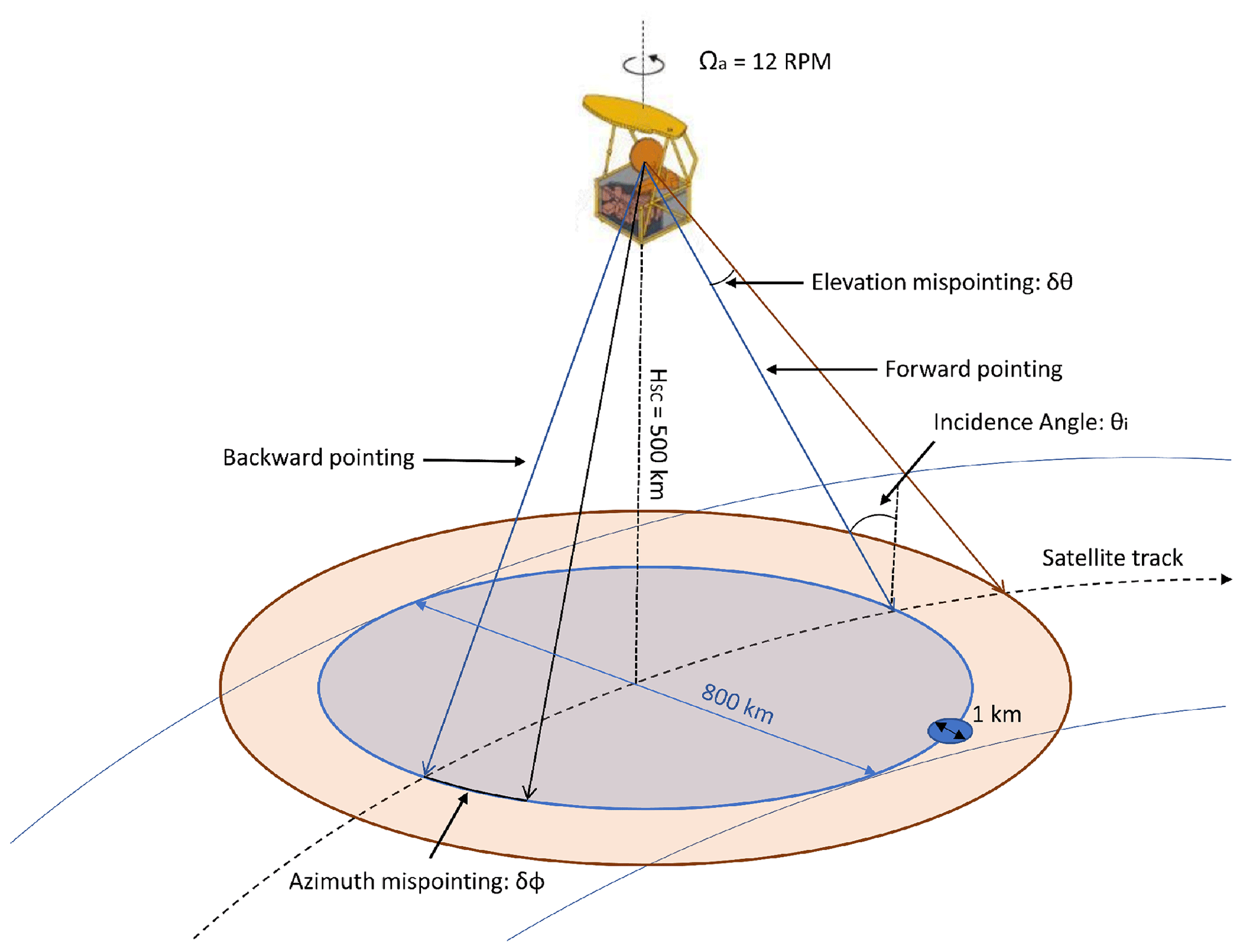
Figure 1 Geometry of observation of the WIVERN conically scanning radar: the antenna boresight, indicated by a thin blue line, is rotating at 12 rpm and pointing at a nominal incidence angle of about 42^∘. The orange arrow and the black arrow represent an elevation and an azimuthal mispointing in correspondence to the forward and backward pointing configuration, respectively.

Table 1 Specifics of the WIVERN radar. The configuration adopted herein is the one currently under phase-0 study for the ESA Earth Explorer 11 programme.

3 Doppler velocity correction methods

Four different methods have been identified that can be used to correct Doppler velocity errors. Methods II and III are applicable both to azimuth and elevation mispointing, method I is applicable only to elevation mispointing and method IV only to azimuthal mispointing; the first two (I and II) are effective on short timescales (of the order of a few milliseconds), the latter two (III and IV) on much longer timescales (weeks or months).

3.1 Correction method I: altimeter mode technique

Because of its peculiar illumination geometry, pulse shape and the receiver IF filter response (Meneghini and Kozu, 1990), the WIVERN radar will produce a very specific reflectivity shape for flat surfaces in the absence of low level clouds and/or precipitation, with a peak corresponding to the surface range along the boresight direction (Battaglia et al., 2017; Illingworth et al., 2020). Since the position of the spacecraft is extremely well known, any discrepancy, δz, between the range of the surface from the spacecraft computed along the (attitude and orbital control system (AOCS) – estimated) boresight direction and the measured range of the surface peak can be attributed to an elevation mispointing, δθ, from

$$\begin{array}{}\text{(2)}& \mathit{\delta }\mathit{\theta }={\displaystyle \frac{\mathit{\delta }z}{r_{\text{SC}}\sin {\mathit{\theta }}_i}}\approx {\displaystyle \frac{\mathit{\delta }z\cos {\mathit{\theta }}_i}{\sin {\mathit{\theta }}_i{H}_{\text{SC}}}},\end{array}$$

where r_SC is the distance between the surface and the spacecraft along the boresight and H_SC is the spacecraft altitude. With the WIVERN specifics (see Table 1), δz=10 m corresponds to about 22.5 µrad. Unfortunately, this method is not viable for tackling the azimuth mispointing but has the advantage that it depends only on the reflectivity profile, and thus it has the same sensitivity in each part of the scan.

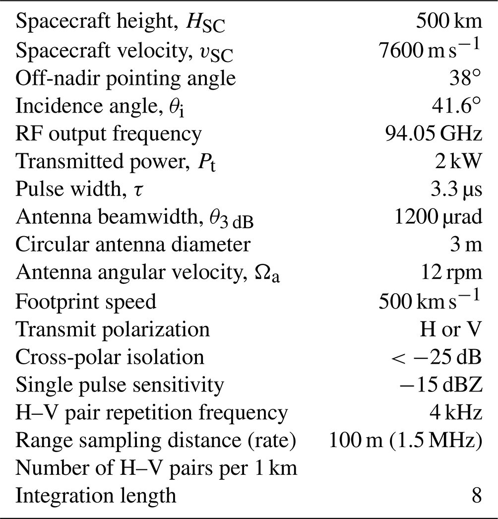
In order to understand the uncertainties associated with this method, realistic surface returns (an example of a surface return is shown as a black line in Fig. 2) as detected by WIVERN have been simulated starting from the expected flat surface return shape derived following Meneghini and Kozu (1990) (also see Fig. 5 in Illingworth et al., 2020). The profiles have been scaled in order to produce different peak to noise ratios (PNR), defined as the ratio between the peak reflectivity of the surface profile and the single pulse sensitivity or reflectivity equivalent noise level of the radar, assumed to be equal to −15 dBZ. For each PNR and each integration length (with eight independent pulses per kilometre), different stochastic realizations of the signal plus the noise are simulated following the technique proposed by Zrnic (1975). One of such possible realizations is shown as the dashed orange line in Fig. 2. Then the signal is noise subtracted (similarly to the method described in Kollias et al., 2023) and sampled at the WIVERN sampling rate (100 m along the range; see Table 1) with random range offsets in order to account for the variability of the digitization process along the orbit (red diamonds in Fig. 2). A surface detection criterion is introduced. For each profile, only points that are 3 dB above the detection level (red diamonds with black dots inside) are considered. If the profile contains at least 10 consecutive points above the detection threshold, it is then used for fitting the surface return shape with two free parameters: the peak height and the peak amplitude. The fit is performed via a least mean square procedure where each point is weighted by the expected error (error bars in Fig. 2) computed according to the signal to noise ratio (SNR; following Eq. 16 in Battaglia et al., 2022). The best fitting curve (blue line) differs from the actual profile for a shift in height, δz, and a shift in amplitude, δZ. The variability in δz can be statistically retrieved as a function of the PNR by generating a sufficient number of profile realizations with different random noise and different digitalizations of the signal. As expected, while the mean value of δz over different digitization and stochastic noise is practically close to 0 m for every PNR and for every integration length (not shown), its standard deviation, σ_δz, decreases when either the PNR and/or the integration length increase, as shown in Fig. 3. The shifts in elevation angle δθ corresponding to the shifting in altitude δz of the peak are reported on the y axis on the right side of Fig. 3. For instance, with a PNR of 10 dB, the surface position is expected to be determined with an error of about 32, 20, 13 and 9 m for integration lengths of 1, 2, 5 and 10 km, respectively. These values correspond to an uncertainty in elevation of 75, 47, 39 and 20 µrad. According to Eq. (1), the last three solutions guarantee that the velocity error induced by such mispointing will always remain below 0.3 m s⁻¹.

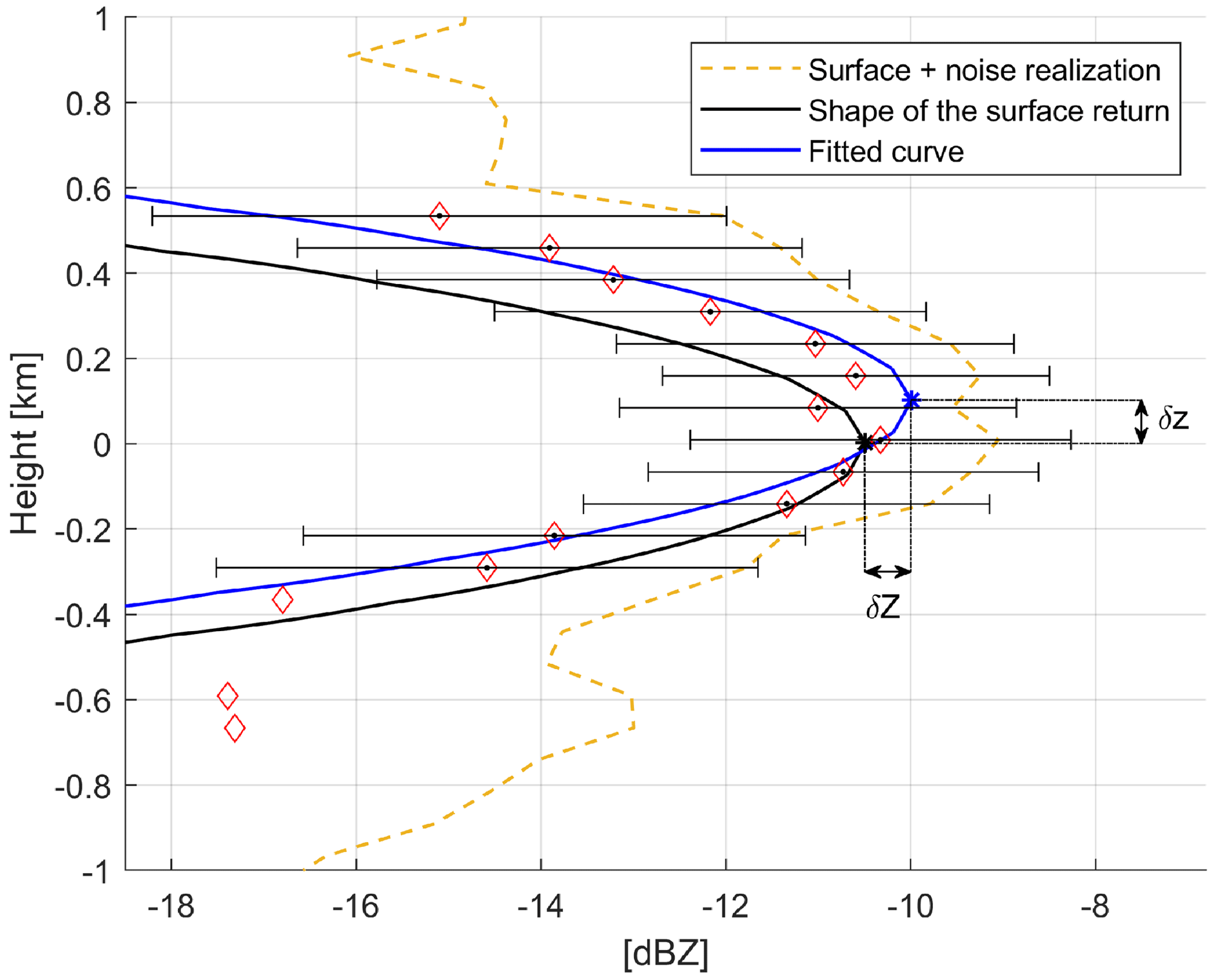
Figure 2 A reflectivity surface profile simulated as observed by the WIVERN radar with the procedure to determine the vertical displacement δz of the peak of the noisy sampled profile with respect to the actual surface peak. The black line represents the ideal shape of the surface return for a 7 dB PNR with its peak highlighted by a black asterisk. The dashed orange line represents a stochastic realization of the same surface return with a −15 dBZ random noise. The red diamonds represent the digitized signal after noise subtraction with the error bars indicating the expected errors in the reflectivity estimates. The black dots insides the red diamonds correspond to the points sampled by the radar that are used for fitting the surface profile. The blue line is the best fitting profile, with the peak highlighted by a blue asterisk. The displacements in height (δz) and in amplitude (δZ) between the black and blue asterisks are indicative of the uncertainties associated with the clutter characterization.

Figure 3 Uncertainty in the elevation mispointing determination by the altimeter mode technique: standard deviations of δz, σ_δz (left axis) and δθ (right axis) as a function of the PNR for different integration lengths, as indicated in the legend. The mean values of δz are negligible for all analysed PNR and integration lengths (not shown). The curves are drawn only for PNRs high enough that more than 80 % of the profiles satisfy the surface detection criteria (See the text for more details.)

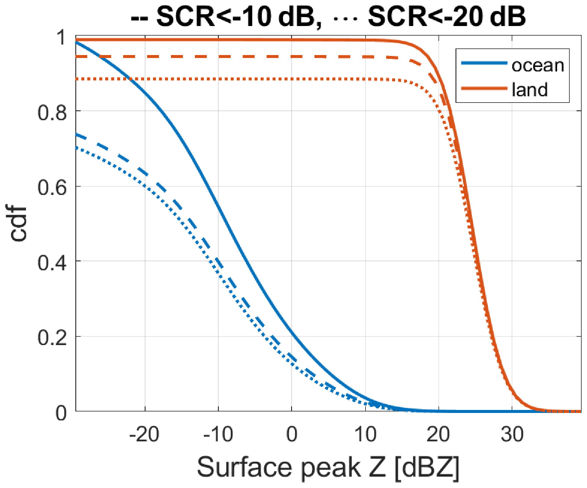
Figure 4 Cumulative distributions of surface reflectivity peaks as expected in WIVERN observations for land (red) and ocean (blue) surfaces. Dashed and dotted lines correspond to rays characterized by decreasing signal to clutter ratios. (See the text for more details.)

3.1.1 Statistics of useful surface return

Estimates of the frequency of surfaces exceeding threshold values of PNR have been obtained by exploiting the climatology gathered by the polar-orbiting nadir-pointing CloudSat W-band radar and simulating the WIVERN returns at slant incidence angle. The method, proposed by Battaglia et al. (2018) and refined in Tridon et al. (2023), accounts for the additional path integrated attenuation and the reduction in surface normalized backscattering cross sections (Battaglia et al., 2017) when considering the slanted viewing geometry of the WIVERN radar. Figure 4 shows the cumulative distribution functions (CDF) of the surface peaks (and equivalently of PNR) for land and ocean surfaces. Since ocean surfaces are far less bright than land surfaces at WIVERN incidence angles, a lower percentage of sea than land surface profiles exceeds any given threshold. For instance, more than 36 % and 99 % of the surface peaks exceed −5 dBZ (i.e. PNR=10 dB) for ocean and land surfaces, respectively. Two factors can actually decrease the number of surface returns effectively useful for the calibration:

1. the presence of low clouds and precipitation that could perturb the shape of the reflectivity and of the Doppler velocity profile (discussed later in Sect. 3.2);

2. for land surfaces, the failure of the flat surface assumption.

In order to assess the first issue, we have recomputed the CDF excluding rays where the hydrometeor signal to clutter ratio (SCR) is higher than −20 dB (dotted lines) and −10 dB (dashed lines) in the 750 m closest to the surface. These conditions ensure that the clutter signal is 100 and 10 times stronger, respectively, than any perturbing signal produced by the hydrometeors. The presence of low clouds will further reduce the number of useful rays for calibration, but such reduction is only of 10 % for SCRs lower than −10 dB and of 13 % for SCRs lower than −20 dB over ocean. Over land, the reduction is even smaller with 5 % and 10 % for SCRs lower than −10 and −20 dB, respectively. (For estimating the impact of the second issue, see the discussion in Sect. 3.2.1.)

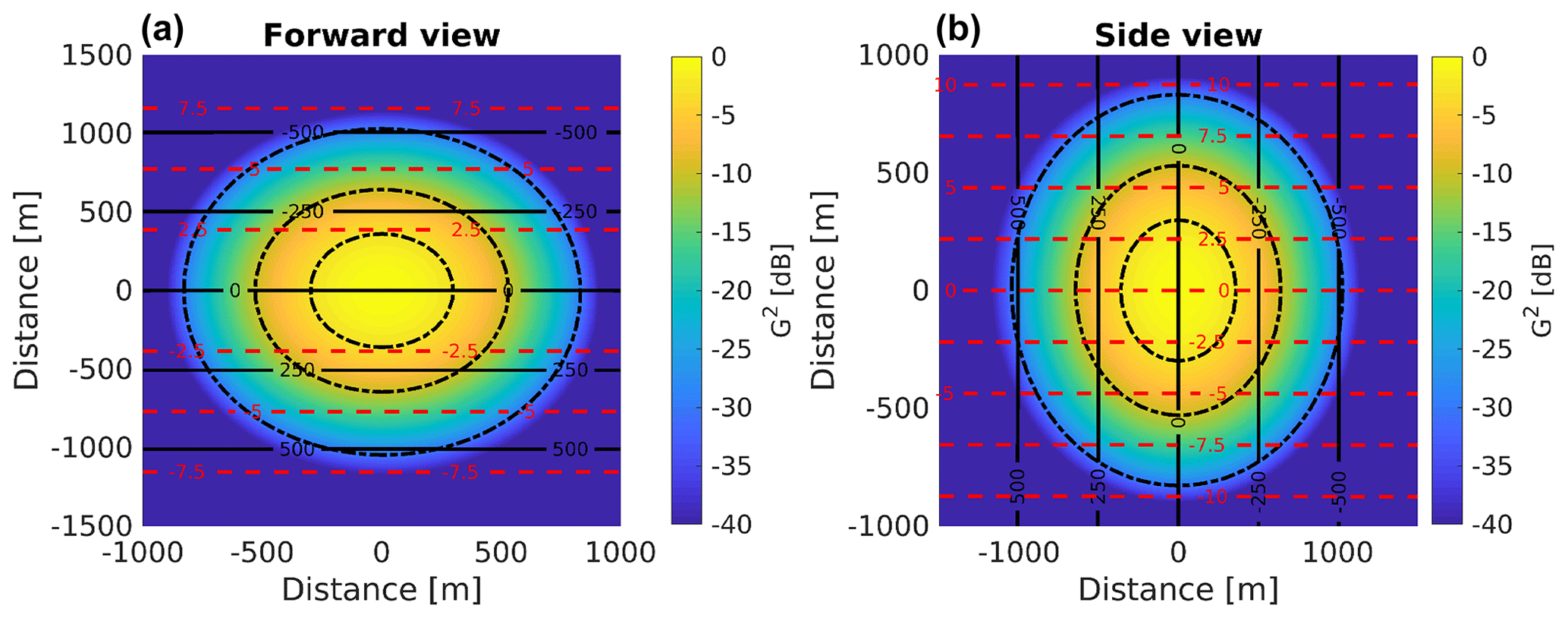
Figure 5 Square of the gain (normalized to 0 dB at boresight) for the WIVERN antenna pattern as derived from a previous study (Lori et al., 2017) for points within 1500 m from the ground projection of the boresight (used as the origin of the coordinate system). Results are reported in correspondence to the (a) forward (ϕ=0) and (b) side ($\mathit{\varphi }=\mathrm{90}{}^{\circ }$) views. In both cases the satellite is assumed to move along the y axis. Contour levels of the satellite velocity along the LOS are plotted as dashed red lines from −10 to 10 m s⁻¹ with 2.5 m s⁻¹ separation, and contour levels of height above the ground are plotted as black lines from −500 to 500 m with 250 m separation. The dotted black curves correspond to −3, −10 and −30 dB of the normalized square gain.

3.2 Correction method II: surface Doppler technique

Flat and still surfaces are characterized by a well-determined Doppler velocity profile. However, while the surface reflectivity profiles are independent of the azimuthal scanning angle, the Doppler velocity profiles are azimuthal dependent. Under the assumption of a homogeneous (i.e. backscattering cross section constant across the footprint) flat and still surface, at side view, the surface Doppler velocity is expected to have 0 m s⁻¹ at all height bins, whereas at other azimuthal angles, positive and negative Doppler velocities are expected above and below the surface with 0 m s⁻¹ only in correspondence to the surface height (black line in Fig. 6). This is the result of the different orientation of the lines of constant Doppler shift induced by v_SC (isodops) with respect to the lines with constant range. As demonstrated in Fig. 5, for the two extreme cases of forward (Fig. 5a) and side (Fig. 5b) views the isodops are parallel and perpendicular, respectively, to the lines of constant range from the radar.

As done in Sect. 3.1, the Doppler returns as measured by the WIVERN radar are simulated with the noisiness proper to the given PNR and the number of independent samples (diamonds in Fig. 6; according to Eq. 16 in Battaglia et al., 2022). Here, a perfect correlation between the V and the H pulse co-polar signals is assumed consistently with low surface LDR values (Wolde et al., 2019). The expected shape (black line) is then fitted through the data that have reflectivities exceeding an SNR of 0 dB via a mean least squares technique. The distance of the fitted profile (blue line) from the expected profile at zero height (δv_D) is indicative of the uncertainty in the Doppler velocity error estimation that can be achieved with this methodology.

Figure 7 shows the Doppler velocity uncertainties associated with this method. In this case, reduction of the error to values lower than 0.4 m s⁻¹ is impractical at short integration lengths (≤2 km) and requires a surface with PNR exceeding 10 and 15 dB for integration lengths of 5 and 10 km, respectively. When comparing the curves at different integration lengths, it can be noted that, approximately, the error drops with the square root of the integration length. Therefore, this technique seems very promising for correcting mispointing modulated on timescales longer than the antenna rotational period. Surface returns for full rotations in correspondence to clear sky and flat surfaces can be used to fit the mispointing error provided by the expression (1). Because of the numerous number of good calibration points (i.e. “flat” surfaces in clear sky with good PNR) expected to be available in different scans, this method will constrain mispointing errors down to less than 0.2 m s⁻¹ within few turns.

3.2.1 Flat surface approximation

The Advanced Spaceborne Thermal Emission and Reflection Radiometer (ASTER) global digital elevation model (DEM) (https://asterweb.jpl.nasa.gov/GDEM.asp; last access: 2 June 2023), with a resolution of ${\mathrm{1}}^{\prime \prime }\times {\mathrm{1}}^{\prime \prime }$ (i.e. 30.9 m×30.9 m at the Equator), has been used to examine the validity of the flat surface assumption by evaluating the variability of the elevation in areas comparable to that swept by the WIVERN radar footprint with different integration lengths. Boxes with latitudinal extent of 18^′′ and longitudinal extents of 18, 36, 72, 90 and 180^′′ were considered, which corresponds roughly to from no integration to 5 km integration length. The standard deviations of the elevation, σ_elev, within each box were then calculated for the entire global data set. Figure 8 shows the variation of the cumulative land fraction with σ_elev, for the five box sizes adopted. The respective values of σ_elev for increasing box size, given in the form (50th percentile, 70th percentile, 90th percentile), are (7.0 m, 12.0 m, 37.3 m), (8.0 m, 14.4 m, 47.1 m), (9.4 m, 17.9 m, 59.5 m), (10.0 m, 19.2 m, 63.5 m), and (12.0 m, 23.6 m, 74.9 m). It is clear that, for a given percentile, the value of σ_elev increases as the box size increases. These findings suggest that roughly half of the land surfaces have a variability in elevation less than 10 m within characteristic WIVERN averaging areas. Such surfaces will likely be useful for the calibration methods I–II (Sects. 3.1 and 3.2), but a dedicated study to properly assess the impact of surface elevation variability is needed.

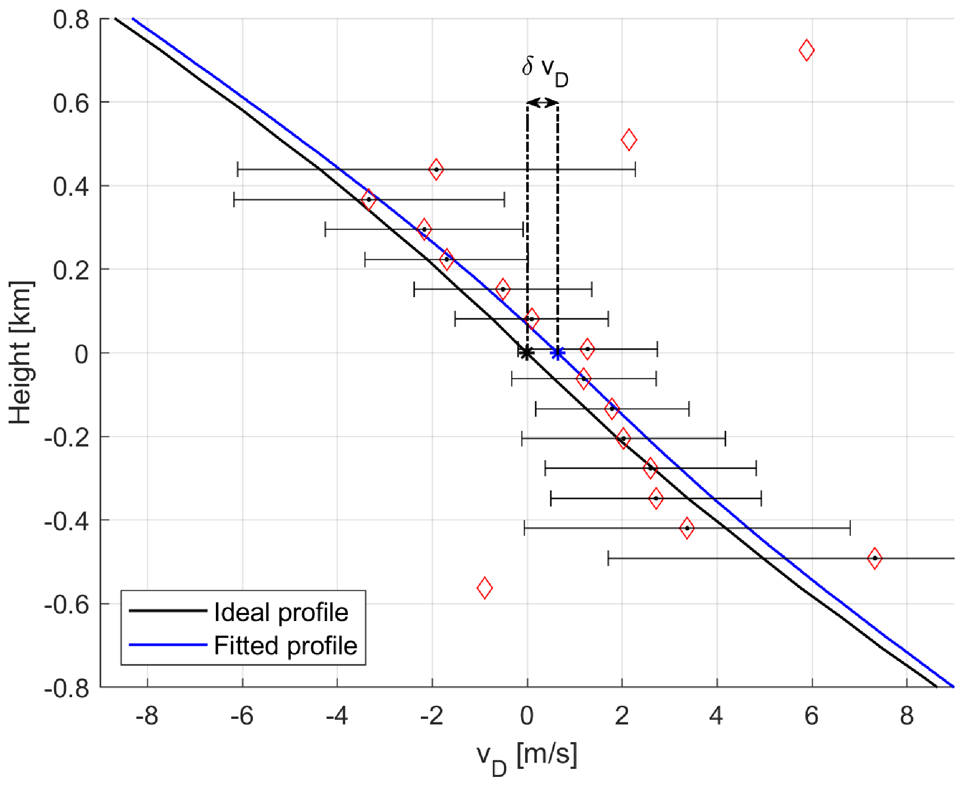
Figure 6 A Doppler velocity profile of the surface simulated for WIVERN observations in the forward direction. The black line represents the ideal Doppler velocity profile without the noise. The red diamonds are the points of the noisy Doppler velocity profile that are oversampled by the radar (one point every 100 m along the LOS). The black dots identify the points of the noisy profile with reflectivities above the detection level. Such points are fitted with the shape of the surface return in order to produce the blue line. The Doppler velocities represented by the blue line are the ones retrievable from the radar measurements and they differ from the ideal velocities due to the presence of the noise. δv_D is the velocity shift in correspondence to the surface induced by the noise in the retrieved profile.

A final consideration is that, generally, ocean surfaces will not appear to have zero Doppler velocities, but they will have biases of the order of less than 1 m s⁻¹. This is due to the interplay between waves and currents (Chapron et al., 2005; Ardhuin et al., 2019). Here it is assumed that corrections for such effects can be performed based on auxiliary information or that they will average out when considering views from different directions.

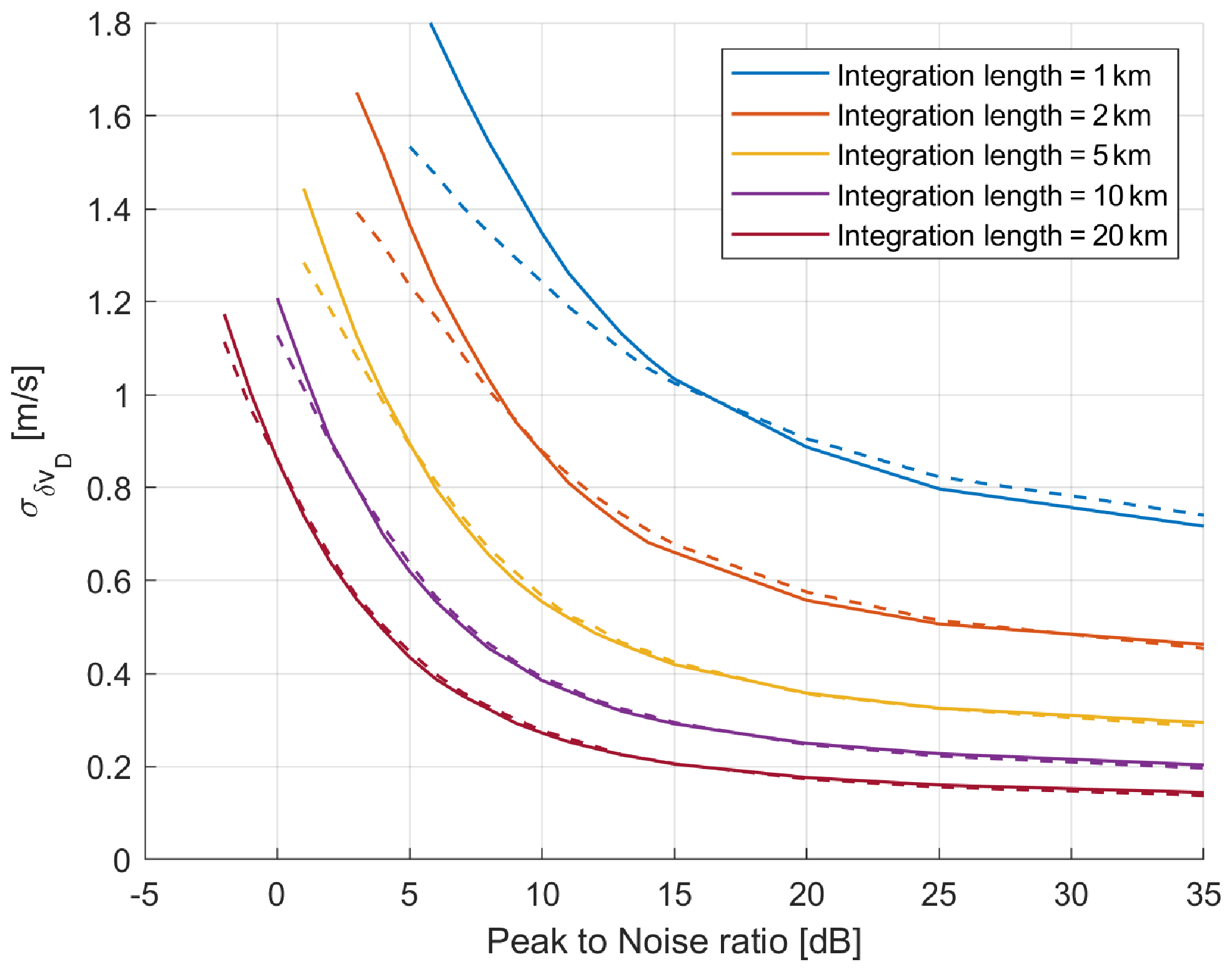
Figure 7 Doppler velocity uncertainty associated with the surface Doppler technique for forward pointing (i.e. azimuthal angle = 0^∘; solid lines) and side pointing (i.e. azimuthal angle = ±90^∘; dashed lines) (but similar results are found for any azimuthal angle). The standard deviations of δv_D are plotted as a function of the PNR for different integration lengths as indicated in the legend. The variability of δv_D decreases as the PNR and/or the integration length increase. The mean values of δv_D are negligible for every PNR and every integration length herein analysed (not shown). The curves are drawn only for PNRs high enough that more than 80 % of the profiles satisfy the surface detection criterion. (See the text for more details.)

3.3 Correction method III: active radar calibrator techniques

The use of active radar calibrators (ARC) is well established for external calibration of SAR instruments. It has been applied for calibrating the TRMM and GPM radars as well (Masaki et al., 2022).

Here we only consider the use of the ARC in receiver mode with extremely high sampling resolution (≤0.1 µs). Like in Masaki et al. (2022) we assume the ARC beamwidth to be of the order of 20^∘ and thus much larger than the WIVERN beamwidth. Then, in relation to an overpass, if the ARC is pointed toward the satellite, the power received by the ARC at the sampling time t_k, P_ARC(t_k), is effectively determined only by the WIVERN Tx antenna pattern. Typically, the signal at the ARC will be detectable for a few tenths of milliseconds (Fig. 9b). Since the velocity of the spacecraft is very low with respect to the scanning velocity of the radar, its effect on the relative motion of the ARC inside the antenna pattern is negligible. Thus, all the possible trajectories of the ARC inside the pattern always look like a slightly bent line extended along the azimuth distance (Fig. 9a).

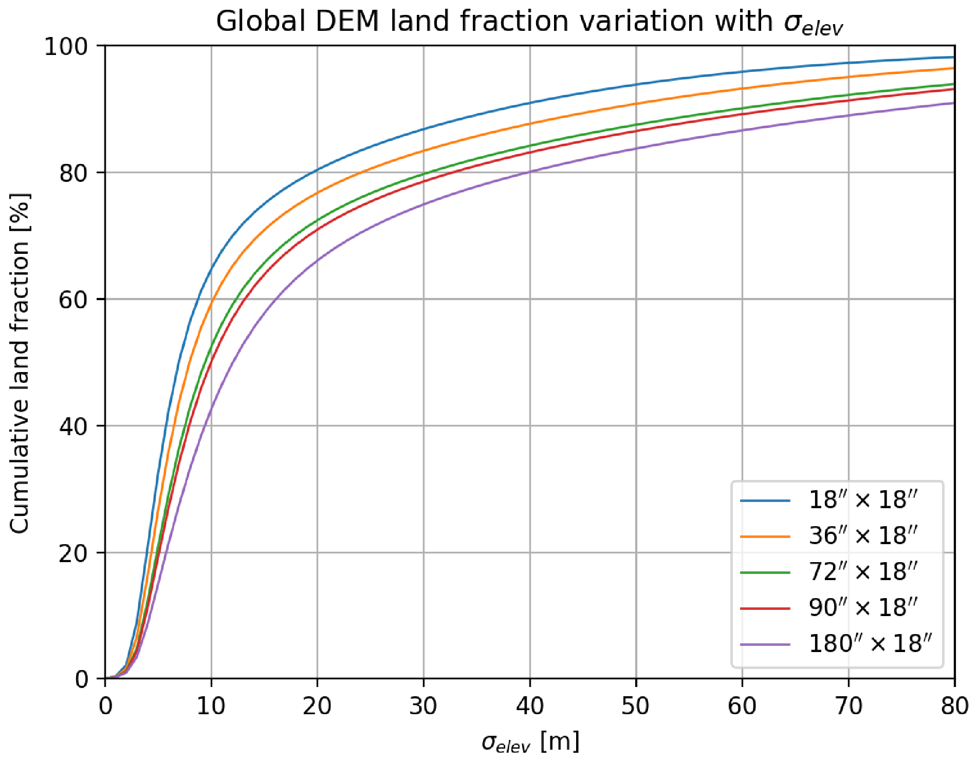
Figure 8 Variation in the cumulative land fraction from the ASTER global digital elevation model (DEM) with σ_elev for different latitude and longitude box sizes. Each coloured line corresponds to a particular longitude × latitude box size (indicated in the legend).

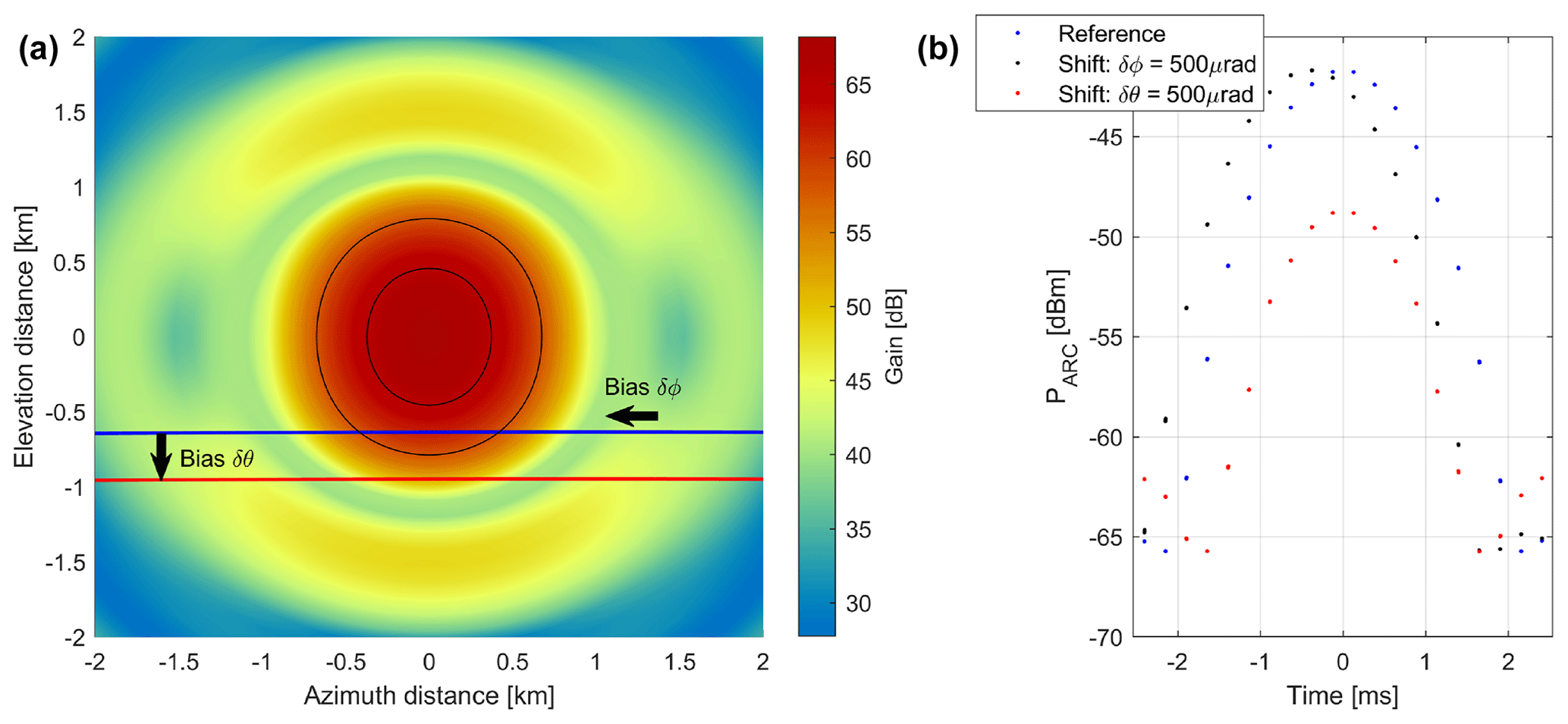
Figure 9 Panel (a) shows an example of how the ARC position (expressed in terms of distances at the ground) moves inside the WIVERN antenna pattern when a bias in elevation or in azimuth of 500 µrad is introduced. The satellite is located along the negative y axis with the antenna pointing forward in the y direction. The blue line is the position of the ARC for a scanning with a minimum distance between ARC and boresight position of 635 m (reference). The red is the same scan shifted by 500 µrad in elevation bringing the minimum distance between the ARC and the antenna boresight position to 950 m. Solid black lines correspond to the contour levels of the antenna gain 3 and 10 dB below the maximum gain. Panel (b) shows the ARC received power for the reference (blue) and the scans shifted by 500 µrad in elevation (red) and in azimuth (black). The power received is sampled every 0.1 µs and 3.3 µs pulses are transmitted by the radar every 250 µs.

Note that the radar receiver chain can also be tested by using the radar as an active calibrator (e.g. by sending back to the radar a copy of the signal received by the ARC). With this technique the power received at the WIVERN receiver will depend on the product of the antenna gain in receiving and transmitting mode and thus will have a higher sensitivity than the method discussed next.

The geolocation of the ARC, the position of the spacecraft, the propagation time of the signal and the time at which the spaceborne radar send the pulses are assumed to be perfectly known. Uncertainty in the knowledge of those factors affects uncertainty in the mispointing error detection and in the Doppler velocity correction achieved with the ARC technique.

3.3.1 Elevation mispointing

As illustrated in Fig. 9, an elevation mispointing bias moves the apparent motion of the ARC position inside the WIVERN antenna pattern along the elevation direction (y axis), e.g. from the blue to the red line. Note that uncertainties in the atmospheric refraction between different models (Mangum and Wallace, 2015) are expected to be of the order of 1 arcsec (i.e. lower than 5 µrad) and are therefore neglected in this study. Correspondingly, the actual power measured by the ARC, derived by using Friis formula with an ARC gain of 20 dB, changes because of the difference in the antenna pattern. Such change depends on the specific position of the overpass (e.g. on the minimum distance of the boresight position to the ARC) and on the details of the antenna pattern. In order to simulate the capability of the ARC measurement to identify and quantify the mispointing, different possible boresight ground tracks have been simulated (like the blue and the red lines in Fig. 9a). For each ARC position at a given elevation distance $\stackrel{\mathrm{‾}}{\mathit{\theta }}$, the ARC signal is simulated and compared with the returns sampled at different elevation distances $\stackrel{\mathrm{‾}}{\mathit{\theta }}+\mathrm{\Delta }\mathit{\theta }$ (with a maximum shift Δθ of ±1000 µrad and sampled every 5 µrad).

The mean square distances (MSD) of simulated ARC received signals at position $\stackrel{\mathrm{‾}}{\mathit{\theta }}$ and $\stackrel{\mathrm{‾}}{\mathit{\theta }}+\mathrm{\Delta }\mathit{\theta }$ sampled at different time t_k with $k=\mathrm{1},\mathrm{\dots },N_{\mathrm{t}}$ is computed as

$$\begin{array}{}\text{(3)}& \begin{array}{rl}\text{MSD}(\stackrel{\mathrm{‾}}{\mathit{\theta }},\stackrel{\mathrm{‾}}{\mathit{\theta }}+\mathrm{\Delta }\mathit{\theta })=& {\displaystyle \frac{\sqrt{{\sum }_{k=\mathrm{1}}^{N_{\mathrm{t}}}\left(P_{\text{ARC}}^{\stackrel{\mathrm{‾}}{\mathit{\theta }}}\right(t_k)-P_{\text{ARC}}^{\stackrel{\mathrm{‾}}{\mathit{\theta }}+\mathrm{\Delta }\mathit{\theta }}(t_k){)}^{\mathrm{2}}}}{N_{\mathrm{t}}}}\\ & -\mathrm{1000}\mathrm{\mu }\mathrm{rad}\le \mathrm{\Delta }\mathit{\theta }\le \mathrm{1000}\mathrm{\mu }\mathrm{rad}.\end{array}\end{array}$$

All power signals below −80 dBm in the summation have been excluded in order to make sure there will be no effective impact from ARC receiver noise. A 0.5 and 1 dB noisiness is introduced in the antenna pattern to account for uncertainties in the antenna pattern. A total of 400 different realizations of the antenna pattern are used to compute the MSD in Eq. (3) so that a distribution of MSD can be derived for each pair $(\stackrel{\mathrm{‾}}{\mathit{\theta }},\stackrel{\mathrm{‾}}{\mathit{\theta }}+\mathrm{\Delta }\mathit{\theta })$.

The almost symmetric shape of the antenna pattern causes the similarity between two signals sampled at opposite elevation angles with respect to the boresight (i.e. with $\stackrel{\mathrm{‾}}{\mathit{\theta }}=\pm \mathrm{\Delta }\mathit{\theta }$). Two examples of the 50th (line) and 5–95th percentiles (shading) of the MSD pdfs (probability density functions) are shown in Fig. 10 for $\stackrel{\mathrm{‾}}{\mathit{\theta }}=\mathrm{160}$ µrad (Fig. 10a) and $\stackrel{\mathrm{‾}}{\mathit{\theta }}=\mathrm{480}$ µrad (Fig. 10b). As expected, the minimum is found in relation to a shift between the pairs Δθ equal to 0 µrad, but the interplay between the width of the pdf and the prominence of the local minimum introduces uncertainties in the determination of the mispointing.

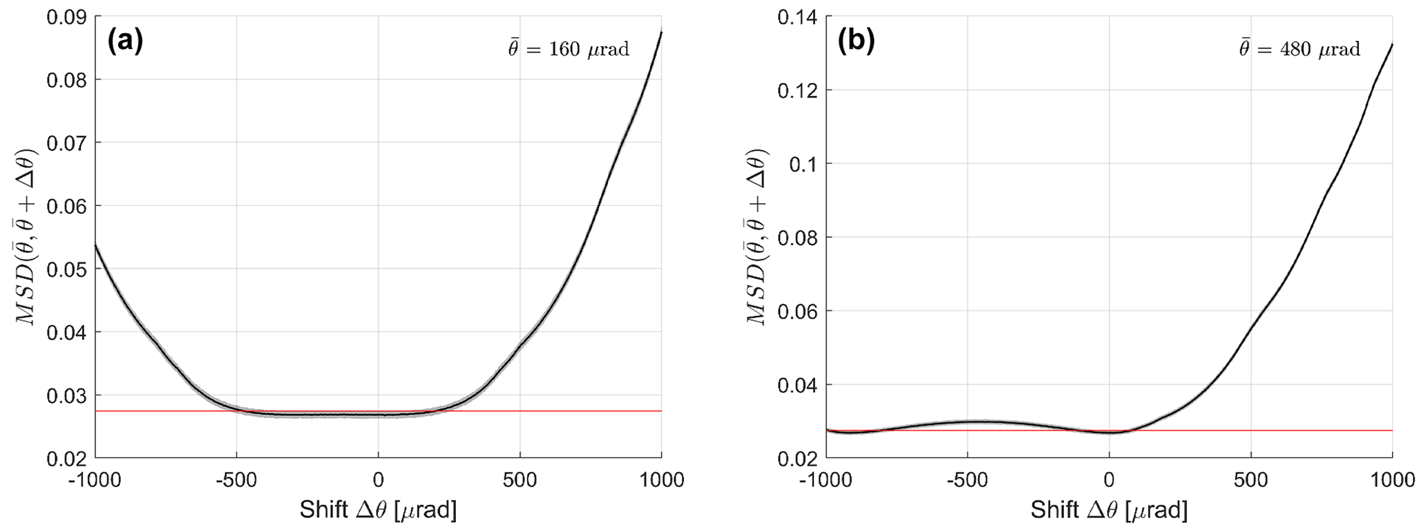
Figure 10 Example of least squares distances (the continuous line corresponds to the 50th percentile, while the shading corresponds to the 5th and 95th percentiles) for 400 different realizations of the antenna pattern with 1.0 dB of uncertainty as a function of the shift in elevation Δθ for an overpass with antenna boresight passing at $\stackrel{\mathrm{‾}}{\mathit{\theta }}=\mathrm{160}$ µrad (a) and at $\stackrel{\mathrm{‾}}{\mathit{\theta }}=\mathrm{480}$ µrad (b) from the ARC.

When considering an overpass close to the ARC (e.g. $\stackrel{\mathrm{‾}}{\mathit{\theta }}=\mathrm{160}$ µrad; Fig. 10a), the same MSDs are encountered on a vast interval of Δθ, ranging inside the first antenna main lobe in a symmetric way, i.e. with θ between $-\stackrel{\mathrm{‾}}{\mathit{\theta }}-\mathrm{\Delta }\stackrel{\mathrm{‾}}{\mathit{\theta }}$ and $\stackrel{\mathrm{‾}}{\mathit{\theta }}+\mathrm{\Delta }\stackrel{\mathrm{‾}}{\mathit{\theta }}$ with $\mathrm{\Delta }\stackrel{\mathrm{‾}}{\mathit{\theta }}=\mathrm{250}$ µrad for this specific example. When considering ARC positions farther away from the boresight, a second local minimum may form with regard to $\mathrm{\Delta }\mathit{\theta }=-\mathrm{2}\cdot \stackrel{\mathrm{‾}}{\mathit{\theta }}$ (e.g. for $\stackrel{\mathrm{‾}}{\mathit{\theta }}=\mathrm{480}$ µrad, the second local minimum is at around $\mathrm{\Delta }\mathit{\theta }=-\mathrm{960}$ µrad; Fig. 10b).

Figure 11a shows the uncertainty in the elevation mispointing determination as a function of the elevation distance of the ARC from the WIVERN antenna boresight. It is determined by computing for which elevation mispointing the upper 95th percentile, corresponding to the minimum of the MSD (level identified by the red line in Fig. 10), exceeds the lower 5th percentile in the adjacent mispointing angles. The black and the red shading represent the result obtained considering an antenna pattern uncertainty of 0.5 and 1.0 dB, respectively. Results show that uncertainty is maximized in correspondence to an overpass of the boresight exactly over the ARC.

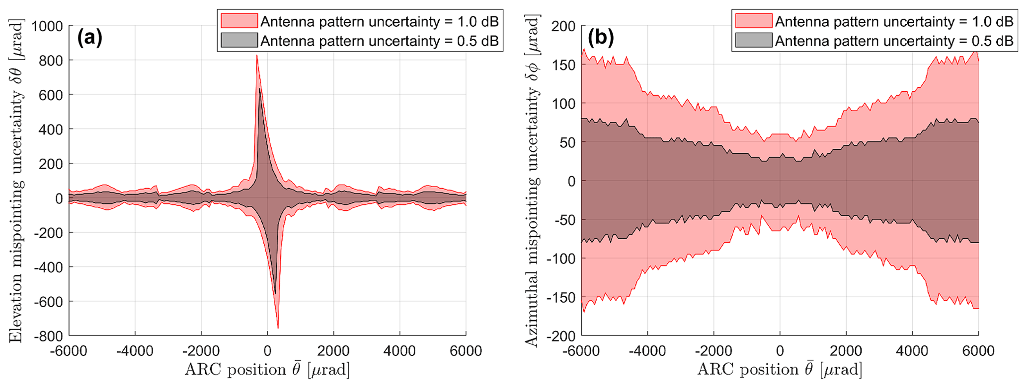
Figure 11 Uncertainty in the elevation (a) and azimuthal (b) mispointing determination as a function of the minimum ARC elevation distance, $\stackrel{\mathrm{‾}}{\mathit{\theta }}$, from the WIVERN antenna boresight. Cases with 0.5 dB (black) and 1.0 dB (red) uncertainty in the antenna pattern are shown.

Given the fact that there will be more than one overpass each month (see Fig. 12), it seems realistic to bring this uncertainty down to less than 50 µrad.

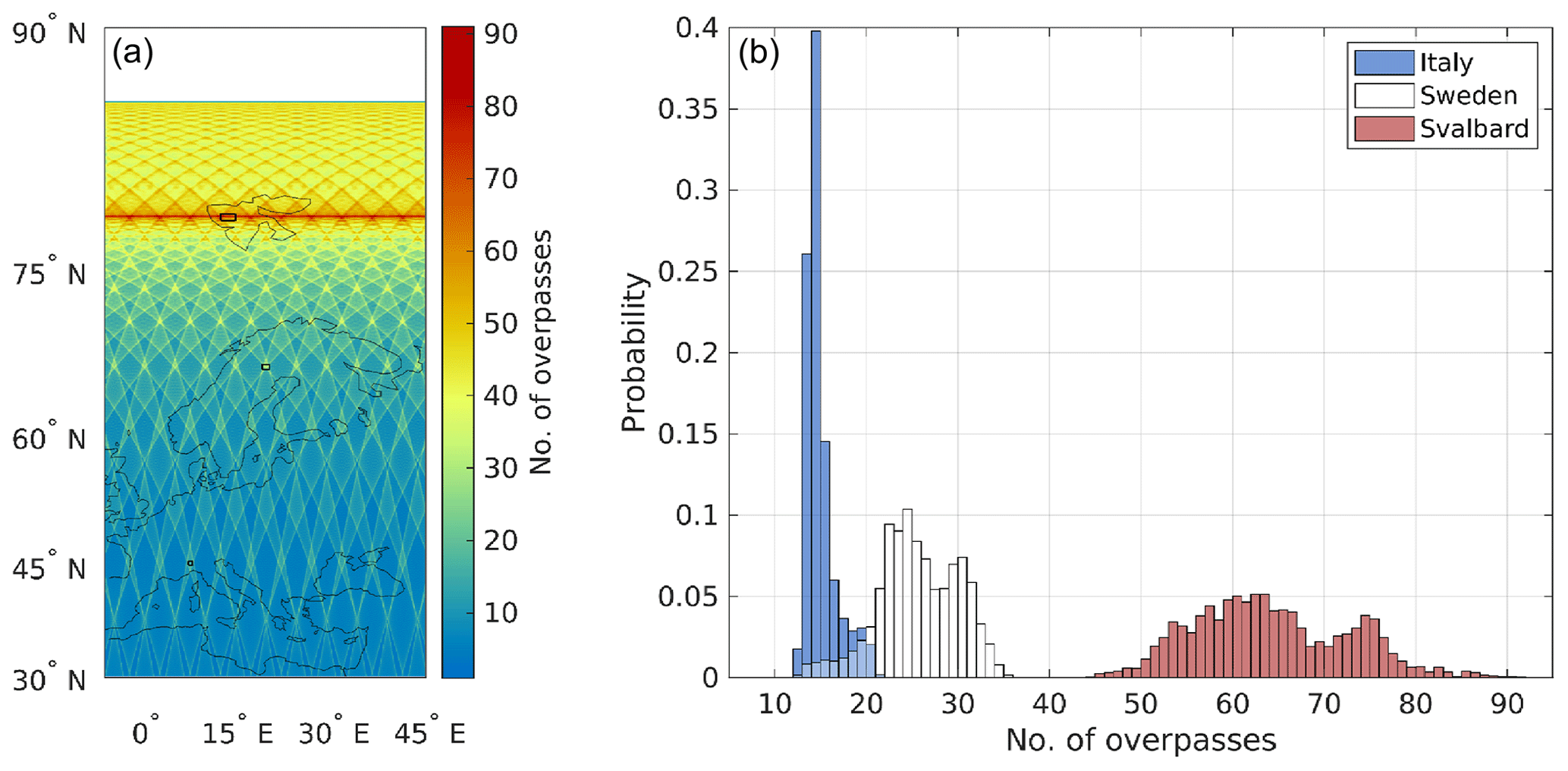
Figure 12 Panel (a) shows ARC average number of overpasses within the 10× beamwidth footprint over 10 d. Panel (b) shows a histogram of the number of overpasses for the selected 50 km×50 km regions (black rectangles in (a)).

3.3.2 Azimuthal mispointing

On the other hand, a mispointing in azimuth does not move the apparent motion of the ARC position inside the WIVERN antenna pattern (Fig. 9), but only translates the received power at the ARC in time. The transmission time and flight time of the radar pulses (∼2.2 ms) are well known; excess path lengths in the atmosphere are expected to be less than a few metres, and thus delays are expected to be of the order of less than 0.01 µs, negligible in this context (Mangum and Wallace, 2015). The procedure followed for the elevation mispointing is replicated introducing a shift in azimuth, Δϕ. In this case,

$$\begin{array}{}\text{(4)}& \begin{array}{rl}\text{MSD}(\stackrel{\mathrm{‾}}{\mathit{\theta }},\mathrm{\Delta }\mathit{\varphi })=& {\displaystyle \frac{\sqrt{{\sum }_{k=\mathrm{1}}^{N_{\mathrm{t}}}\left(P_{\text{ARC}}^{\stackrel{\mathrm{‾}}{\mathit{\theta }}}\right(t_k)-P_{\text{ARC}}^{\stackrel{\mathrm{‾}}{\mathit{\theta }}}(t_k+\mathrm{\Delta }\mathit{\varphi }/{\mathrm{\Omega }}_{\mathrm{a}}){)}^{\mathrm{2}}}}{N_{\mathrm{t}}}}\\ & -\mathrm{1000}\mathrm{\mu }\mathrm{rad}\le \mathrm{\Delta }\mathit{\varphi }\le \mathrm{1000}\mathrm{\mu }\mathrm{rad}.\end{array}\end{array}$$

As before, pdfs of MSD are computed and an estimate of the uncertainty in the azimuthal mispointing is derived based on percentiles. The right panel of Fig. 11 shows that the closer the overpass is to the ARC, the lower is the uncertainty in the azimuthal mispointing determination.

3.3.3 Expected number of useful calibration points as a function of ARC locations

The previous methodology requires the ARC to be positioned in a location within a few kilometres (a few thousand µrad) from the radar boresight location at the ground. To estimate the number of useful calibration points as a function of ARC locations, the WIVERN orbit and boresight positions have been propagated for 50 d. Although the satellite ground track has a repeat cycle of 5 d, the boresight will not trace the same path after this period, and thus different regions will be observed within the swath. The simulation rationale consists of selecting a distribution of ARC locations over the region of interest (Fig. 12a) and counting the number of overpasses within a given footprint. A 1 km spacing in latitude and longitude has been selected to generate the ARC distribution over the region, whereas a time step of 0.5 ms (equal to 250 m along the scan track) has been selected to guarantee a good sampling of the scan track. The simulation has been repeated considering the footprint corresponding to 1, 3, 5 and 10 times the antenna beamwidth.

Figure 12 shows the average results for a 10 d period obtained from the 50 d simulation. Figure 12a displays the number of overpasses over the selected ARCs for a 10× beamwidth footprint. The image shows several hotspots located at specific latitudes and longitudes, while an optimal longitude-independent cluster of hotspots (red line) exists at around 79^∘ of latitude. Since the enhanced number of overpasses at such locations is generated by the intersections occurring at the lower border of the swath, their positions are around 400 km south of the satellite ground track when it reaches its highest latitude. Three 50 km×50 km regions have been selected around some of the hotspots at latitudes 45, 66.5 and 78.7^∘. Figure 12b shows the histogram of the overpasses within these regions, considering the 10× beamwidth footprint. As expected, a greater number of overpasses occur when moving toward higher latitudes.

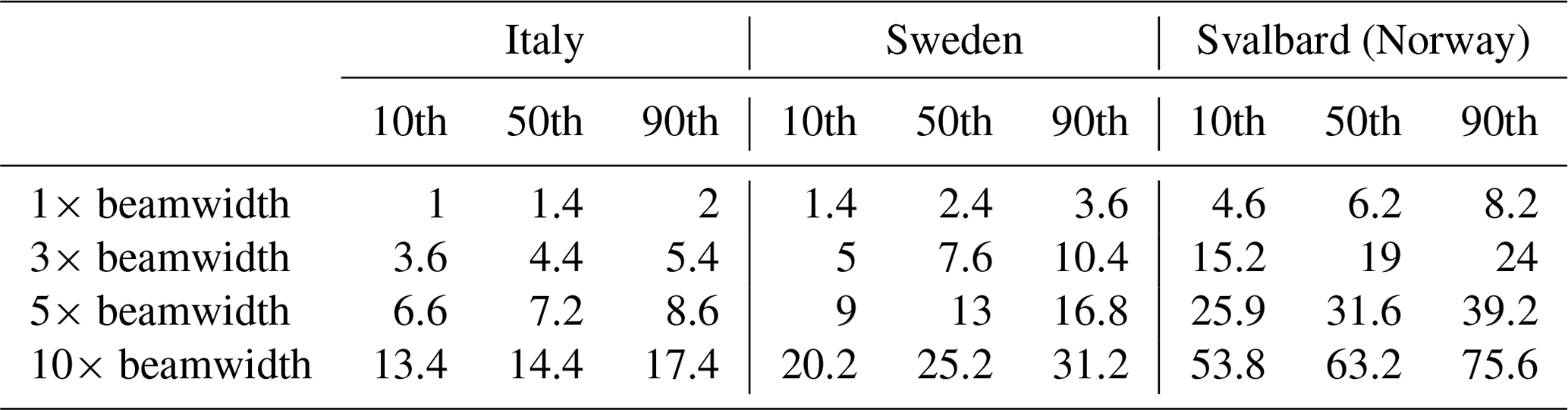
Table 2 summarizes the results when taking different beamwidths. Clearly, when considering the 10× beamwidth footprint (i.e. within roughly 6000 µrad), a sensible number of overpasses (from at least more than 13 at 45^∘ latitude to more than 53 at 78.7^∘ latitude for a 10 d period) is possible over sites whose latitudinal position is properly selected.

Table 2 The 10th, 50th and 90th percentiles of the overpasses for the three selected regions over 10 d. The results refer to the overpasses within the footprints corresponding to 1, 3, 5 and 10 times the beamwidth.

3.4 Correction method IV: ascending and descending orbit and ECMWF reference techniques

During a full rotation, the WIVERN instrument will look at the same LOS for azimuthal angles differing by 180^∘. In such conditions, Eq. (1) predicts that the errors introduced by an azimuthal mispointing will be equal and opposite. But since these are errors in the LOS and the two directions considered here are opposite, this means that the two errors will be identical. Now, for instance, in the part of the orbit closer to the Equator, all winds observed at side views (i.e. with $\mathit{\varphi }=\mathrm{90}{}^{\circ }$, 270^∘ where the impact of the azimuthal mispointing is maximum) roughly correspond to the zonal winds. Then, in the presence of an azimuthal mispointing that is changing at frequencies much lower than the orbital frequency ($f=\mathrm{1.76}\times {\mathrm{10}}^{-\mathrm{4}}$ s⁻¹), the ascending and descending orbits will see opposite biases for the zonal winds (but this is true also for winds in any other direction, though the effect will reduce to zero when observing the meridional winds because of the sin ϕ modulation). The advantage of side views is also that at such angle the elevation mispointing is irrelevant (because of the cos ϕ modulation). Therefore, in the presence of a mispointing δϕ, the two pdfs of ascending and descending zonal winds collected at side views will be shifted by ±v_SCsin θδϕ (i.e. the relative bias between ascending and descending orbits is about 1 m s⁻¹ for δϕ=100 µrad).

Statistically, after several orbits the two pdfs are expected to converge to the same pdf under the assumption that the zonal winds at local times differing by 12 h are the same. Is this assumption correct? In this case, any discrepancy between the two pdfs will be a signature of an azimuthal mispointing. But what is the sensitivity of this methodology? In other words, how long is it necessary to average in order to overcome the natural variability, and what is the detectable bias for a given timescale?

Alternatively, all H-LOS winds can be compared with ECMWF background forecast winds (CloudSat Data Processing Center, 2022), which have been proved to be unbiased (biases are ≤0.3 m s⁻¹ in zonal wind and ≤0.15 m s⁻¹ in meridional winds), have good precision (standard deviations of the order of 2.5 m s⁻¹ mostly because of unresolved small scale variability; Rennie, 2022) and have been exploited to correct Aelous wind biases (Weiler et al., 2021). Each WIVERN H-LOS wind can be subtracted from the ECMWF reference. If WIVERN quality controlled winds are unbiased, then the distribution of the difference should have zero mean; otherwise, the bias could be estimated with an error which will be equal to ${\mathit{\sigma }}_{\text{WIVERN-ECMWF}}/\sqrt{N_{\text{winds}}}$, where σ_WIVERN-ECMWF is the standard deviation of the distribution of the differences and N_winds is the number of independent winds.

3.4.1 CloudSat-based analysis

To address these questions the data set produced in Tridon et al. (2023) that combines the CloudSat reflectivity observations and the ECMWF winds has been exploited. Since CloudSat is orbiting in a sun-synchronous polar orbit like the one foreseen for WIVERN, the winds sampled in the ascending and descending orbits have the same statistical variability expected for WIVERN.

Figure 13 shows an example of simulation of WIVERN measurements from a portion of CloudSat orbit through a northeastern Atlantic widespread low which brought a significant amount of precipitation and high winds over Ireland on 19 February 2007. The CloudSat reflectivity curtain (Fig. 13a) is combined with the corresponding ECMWF wind reanalysis (Fig. 13b) to simulate the slant reflectivity (Fig. 13c) and Doppler velocity (Fig. 13d) curtains that would be observed by WIVERN at side view ($\mathit{\varphi }=\mathrm{90}{}^{\circ }$). Because of the slant incidence angle, the WIVERN surface reflectivity is much lower than that of CloudSat apart from over land (see land/sea flag at the top of 13a). In Fig. 13d, the black contour highlights the areas where the WIVERN Doppler velocity accuracy would be better than 2 m s⁻¹.

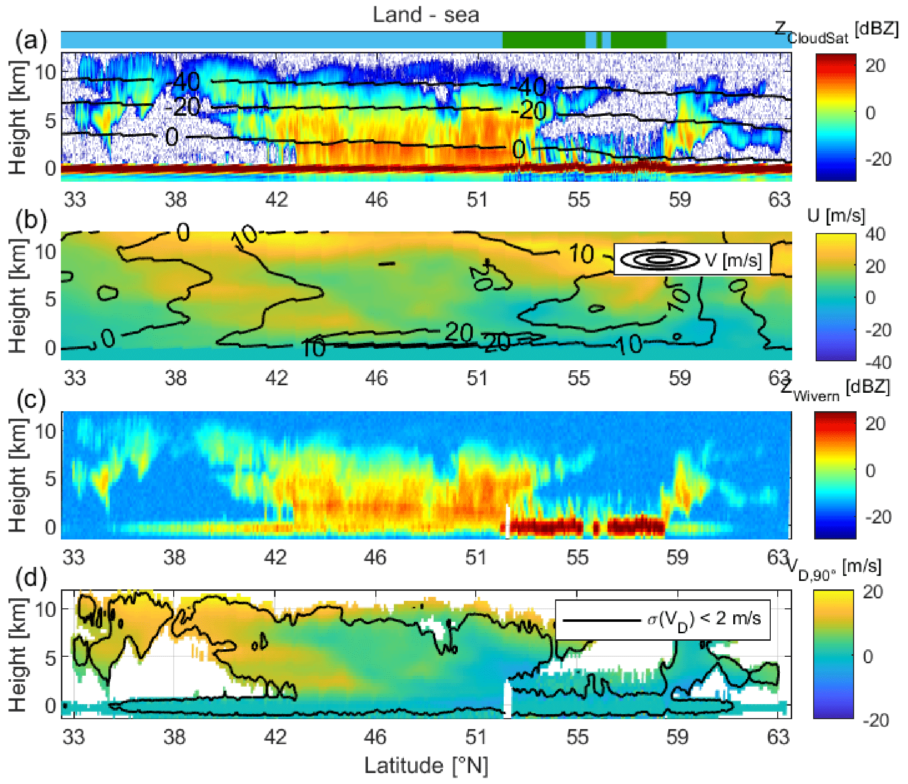
Figure 13 Panel (a) shows CloudSat reflectivity of a frontal system over the eastern Atlantic and British Isles, and ECMWF temperature contours. Panel (b) shows corresponding zonal (colours) and meridional (contours) ECMWF winds. Panel (c) shows simulated WIVERN reflectivity at 10 km resolution. Panel (d) shows a simulated side-view WIVERN Doppler velocity at 10 km resolution with a contour showing areas with an accuracy associated with the radar estimator better than 2 m s⁻¹.

Our method comprises the following steps:

1. The data set has been divided in ascending (A) and descending (D) orbits for latitudes between −65 and 65^∘.

2. Histograms of WIVERN LOS winds when looking sideways to the right/left of satellite in A/D orbits (roughly corresponding to zonal winds) have been accumulated at different heights. Only winds where clouds are present and produce an SNR larger than −4 dB have been considered. Random noise is added to each observation according to the expected error computed from the radar simulator (formula 16 in Battaglia et al., 2022) for integration lengths of 10 km.

3. An ensemble of pdfs of WIVERN “zonal winds” are produced for different integration periods.

4. Jensen–Shannon distances (like in Battaglia et al., 2023) between ascending and descending pdfs computed in step 3 and for A/D pdfs shifted by different wind biases (e.g. ±2 m s⁻¹ corresponding to azimuth biases of 400 µrad).

5. Threshold values expressed in terms of integration time or number of measured winds where different bias levels become detectable according to the Jensen-Shannon distances computed in step number 4 (like in Battaglia et al., 2023).

The pdfs of in-cloud horizontal winds retrieved by WIVERN when looking sideways are shown in Fig. 14a for A/D orbits (diamond/asterisk markers) and for different height ranges as indicated in the legend. The same plot is repeated on the right side considering all-sky condition winds. In the latter condition, A and D wind distributions looks pretty much identical. However, when considering only in-cloud winds, the two distributions take different shapes, suggesting the existence of a diurnal cycle (A and D winds are sampled 12 h apart) affecting in-cloud winds. This result makes the option of identifying azimuthal mispointing only by using WIVERN ascending and descending measurements challenging because the pdfs of A/D in-cloud winds are intrinsically different, and therefore large biases in the winds (typically of the order of 1 m s⁻¹, i.e. ϕ≈200 µrad) are needed to see a neat separation between the two pdfs for accumulation times of at least 10–15 d (not shown).

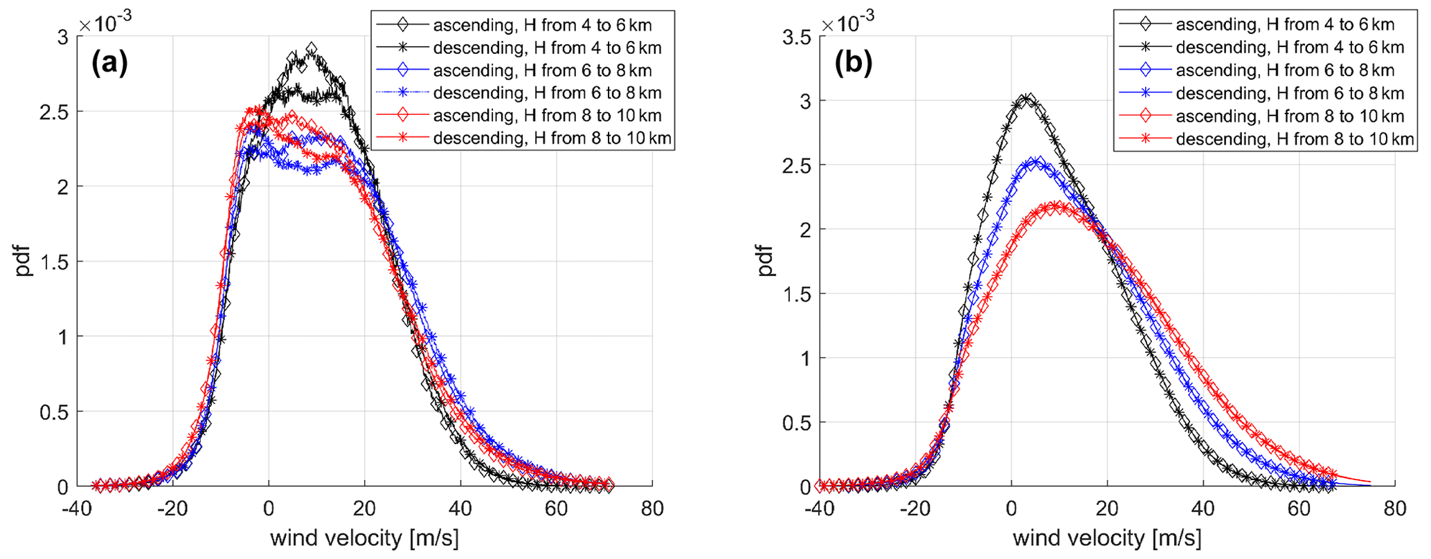
Figure 14 Pdfs of A (diamond marker) and D (asterisk marker) in-cloud horizontal winds retrieved by WIVERN when looking sideways (a) and all-sky-conditions horizontal winds at WIVERN side view (b). In (a), only points characterized by a Doppler velocity accuracy better than 4 m s⁻¹ are considered. The histograms have been generated with points sampled at latitudes within $\pm \mathrm{65}{}^{\circ }$ and at different altitude intervals, as indicated in the legend. The pdfs have been generated with 270 d (in-cloud winds) and 365 d (all-sky winds) of data.

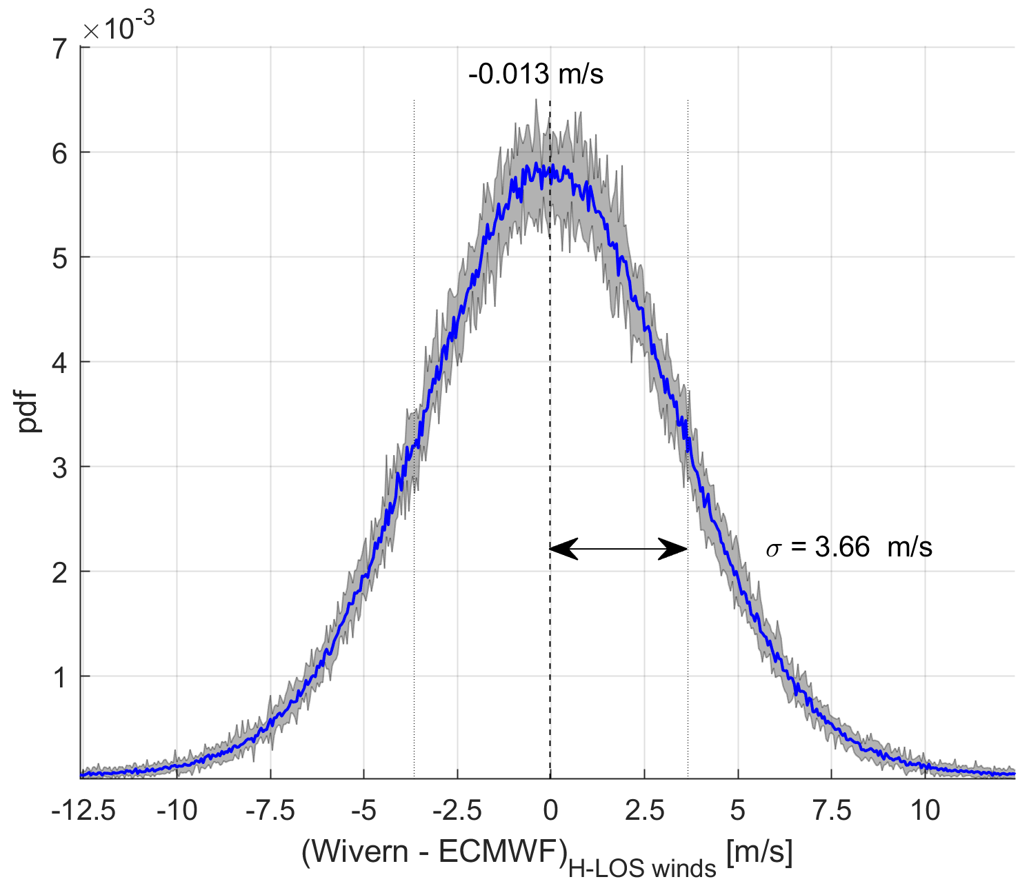
Figure 15 Pdf of the difference between the winds retrieved by WIVERN (LOS) at side view and the ECMWF winds. The pdfs have been generated with 801 474 points, all with an SNR larger than 0 dB, collected during a period of 10 d (blue line). The envelope of the 1 d pdfs collected on each of those 10 d is also shown (grey shading).

On the other hand, when considering the ECMWF as a reference, Fig. 15 demonstrates that the histogram of the differences for the side winds has a standard deviation of the order of 3.66 m s⁻¹ with an average of about 80 000 winds per day. In this case, only WIVERN's wind measurements characterized by an SNR higher than 0 dB have been taken into account. This large amount of winds demonstrates that the error in the estimate of the azimuthal bias will become negligible (≤0.2 m s⁻¹) already after few minutes. The real limit becomes, in this case, the assumption that the reference ECMWF winds are unbiased. The validity of such an assumption applies to global averages over few days with an upper limit for the bias of circa 0.3 m s⁻¹. Note that the same reasoning can be applied to the forward/backward line of sight winds and therefore to the elevation biases.

4 Summary and conclusions

Different methodologies for correcting mispointing errors in conically scanning Doppler velocity measurements (with focus at the WIVERN configuration, currently under study as one of the Earth Explorer 11 candidate missions) have been discussed. Results show the following:

• The use of radar in “altimeter” mode is very robust for identifying elevation mispointing on very short timescales (a few milliseconds). Depending on the surface peak strength and the integration length, different levels of correction can be achieved; e.g. with a 10 dB peak to noise ratio, less than 20 µrad (50 µrad) can be achieved at 10 km (2 km) integration length. This value corresponds to velocity errors smaller than 0.12 m s⁻¹ (0.28 m s⁻¹). The methodology is limited by the flat surface assumption and by the absence of low atmospheric targets that may contaminate the surface signal. Proper screening to identify these situations must be performed beforehand.

• The surface Doppler velocity profile can be used for correcting both elevation and azimuthal mispointing but with generally worse performance than the previous method. With a 10 dB surface peak to noise ratio errors of 0.4 m s⁻¹ (0.9 m s⁻¹) can be achieved at 10 km (2 km) integration length. The method is likely to produce accurate pointing corrections when making use of the clear sky, high peak to noise ratio flat surfaces encountered across several antenna rotations. Limitations similar to the previous method apply in this instance. Additionally, for ocean surfaces, the potential bias introduced to the Doppler velocity by waves and currents must be accounted for.

• The use of an active radar calibrator is effective in identifying slowly changing mispointing errors (biases) larger than about 50 µrad when considering multiple overpasses over week-long periods with the error mainly driven by the knowledge of the details of the antenna pattern. The location of the ARC can be optimally chosen based on the orbit details, with the goal of maximizing the number of overpasses.

• Winds measured by WIVERN in ascending and descending orbits can be used to detect azimuthal biases but only for large biases (of the order of 200 µrad) on timescales longer than 10 d. On the other hand, because of the huge number of WIVERN wind measurements collected every day, the comparison of the level-2 WIVERN H-LOS wind to a state-of-the-art data assimilation system and forecast model, such as the one provided by ECMWF via the so-called O–B (observation–background) technique, is extremely effective in determining biases. The method is practically only limited by time and spatial scales at which the reference model can be considered unbiased.

Future work should address the impact of the instrument footprint variability of the surface σ₀ (e.g. due to differential attenuation or by surface height variability) for methodologies I and II. The impact of waves and currents on the Doppler velocity measurements should also be established at this high frequency and at slant incidence angles.

Appendix A: Effect of a scan-axis mounting offset

In general, the effect of a scan-axis mounting offset can be considered as well. Let A_roll, A_pitch and A_yaw be the roll, pitch and yaw angles, respectively, which characterize the scan-axis mounting offset. We can assume that these angles are constant in time. The offset will generate a bias in the elevation and azimuthal angles with respect to the case where no offset is present. The mispointing in elevation and azimuthal will be time dependent with harmonics of the antenna angular velocity, Ω_a, according to

$$\begin{array}{}\text{(A1)}& {\displaystyle }\mathrm{\Delta }\mathit{\theta }\left(t\right)& {\displaystyle }=-A_{\text{roll}}\sin \left({\mathrm{\Omega }}_{\mathrm{a}}t\right)+A_{\text{pitch}}\cos \left({\mathrm{\Omega }}_{\mathrm{a}}t\right)\text{(A2)}& {\displaystyle }\mathrm{\Delta }\mathit{\varphi }\left(t\right)& {\displaystyle }=-{\displaystyle \frac{\cos \left({\mathrm{\Omega }}_{\mathrm{a}}t\right)}{\tan \left(\mathit{\theta }\right)}}{A}_{\text{roll}}-{\displaystyle \frac{\sin \left({\mathrm{\Omega }}_{\mathrm{a}}t\right)}{\tan \left(\mathit{\theta }\right)}}{A}_{\text{pitch}}+A_{\text{yaw}}.\end{array}$$

The offset angles can be derived as follows:

• Since offset in roll and pitch induce Ω_a-harmonic mispointing in elevation, A_roll and A_pitch can be identified with method 1. The bias in altitude of the surface position, δz, can be averaged over a period long enough in order to cancel out the mispointing in elevation induced by the antenna (effective at higher frequencies). Then, A_roll and A_pitch can be retrieved from Eq. (2) by looking at the δz at forward/backward and side views for A_roll and A_pitch, respectively.

• A_yaw can be handled as a constant azimuthal mispointing, and thus its effect on the Doppler velocity can be corrected adopting method 2.

The assumption that the scan-axis mounting offset is constant is usually valid for errors in the original mounting or by misalignments generated by post-launch conditions. Finally, note that Eqs. (A1) and (A2) allow us to convert a generic perturbation in roll, pitch and yaw of the platform (e.g. inherent to the spacecraft attitude control) into a mispointing in the antenna azimuth and elevation.