Improved mean field estimates from the Geostationary Environment Monitoring Spectrometer (GEMS) Level-3 aerosol optical depth (L3 AOD) product: using spatiotemporal variability

This study presents advancements in the processing of satellite remote sensing data, focusing mainly on aerosol optical depth (AOD) retrievals from the Geostationary Environment Monitoring Spectrometer (GEMS). The transformation of Level-2 (L2) data, which includes atmospheric-state retrievals, into higher-quality Level-3 (L3) data is crucial in remote sensing. Our contributions lie in two novel improvements to the processing algorithm. First, we improve the inverse-distance-weighting algorithm by incorporating quality flag information into the weight calculation. By assigning weights that are inversely proportional to the number of unreliable grids, the method can provide more accurate L3 products. We validate this approach through simulation studies and apply it to GEMS AOD data across various regions and wavelengths. The use of quality flags in the algorithm can provide a more accurate analysis of remote sensing. Second, we employ a spatiotemporal merging method to address both spatial and temporal variability in AOD data, a departure from previous approaches that solely focused on spatial variability. Our method considers temporal variations spanning previous time intervals. Furthermore, the computed mean fields show similar spatiotemporal patterns to previous studies, confirming their ability to capture real-world phenomena. Lastly, utilizing this procedure, we compute the mean field estimates for GEMS AOD data, which can provide a deeper understanding of the impact of aerosols on climate change and public health.

1 Introduction

In satellite remote sensing missions, observed data are processed at different levels. Using retrievals from the atmospheric-state (Level 2; L2), L2 aerosol optical depth (AOD) products are regridded to Level-3 (L3) products through the processes of gap filling and filtering out noises (Cressie, 2018). We first introduce the theoretical background of the mean field algorithm used to generate L3 data applied to AOD retrievals from the Geostationary Environment Monitoring Spectrometer (GEMS) instrument. We consider an oversampling method for generating L3 AOD data, an inverse-distance-weighting (IDW) algorithm, and a modified mean field algorithm while accounting for spatiotemporal variability in AOD data in the algorithm.

Aerosols play a critical role in radiative forcing, climate change, and air quality (Brauer et al., 2015; Charlson et al., 1992; Stocker, 2013; Kaufman et al., 2002). They directly change the planetary albedo by reflecting solar radiation and absorbing terrestrial radiation, affecting the radiation balance. Indirectly, as cloud condensation nuclei, aerosols modify cloud properties and increase cloud droplet concentration, impacting solar radiation and cloud albedo (Alexander et al., 2013). Aerosols affect human health and air quality, especially in regions affected by long-range transport or regions with heavy aerosol emissions due to rapid industrialization and a high population density. These effects are linked to cardiovascular, respiratory, and allergic diseases, as well as increased mortality rates (Pöschl, 2006; Tager, 2004).

Additionally, high aerosol concentrations can severely reduce visibility, leading to hazardous weather conditions, such as haze, smog, and dust storms (Charlson, 1969; Chen and Tsai, 2001). Thus, understanding the multifaceted impacts of aerosols is crucial for addressing issues concerning climate change, public health, and environmental visibility. The distribution of aerosols is characterized by its complexity, leading to increased uncertainty in determining the radiative-forcing effects of aerosols (Chen et al., 2022). Analyzing the spatiotemporal distribution of aerosols remains crucial for developing air pollution control policies and understanding the climate impacts of aerosols. Although accurate aerosol optical properties (AOPs) and their vertical profiles can be obtained from ground-based measurements with a high temporal resolution, the AOPs only represent local-scale variability with limited spatial coverage. Unlike ground-based instruments, the monitoring of AOPs on regional and global scales has been conducted using satellite measurements.

A previous study by Park et al. (2023) focused on AOD retrievals by considering spatial variability. Specifically, Park et al. (2023) used the IDW algorithm to regrid L2 products and estimated the mean field of L3 products by considering spatial variability. Compared to this previous work, our contributions are as follows. First, we integrate quality flag information into the IDW algorithm to rule out unreliable grid points. In this study, we employ the IDW algorithm to compute mean field estimates for AOD data. The IDW method is a widely used gap-filling algorithms that imputes missing observations through a linear combination of neighboring observations. Integrating quality flags (QFs) as weights into the IDW algorithm allows for a quantitative assessment of the influence of data from various quality levels on the final product. It can mitigate the impact of low-quality data and lead to a lower mean squared error (MSE) when implementing the IDW algorithm, as demonstrated in Sect. 4. By considering variability in L2 AOD products, we can obtain more reliable L3 AOD products in this step. Second, we use the spatiotemporal merging method (Kikuchi et al., 2018) to obtain L3 AOD mean field estimates. Numerous studies have demonstrated that aerosol optical depth (AOD) exhibits significant spatiotemporal variability due to natural and anthropogenic factors. This is particularly evident in regions like northwestern China, where understanding spatiotemporal dynamics is essential for effective atmospheric-pollution management and control as aerosol concentrations are heavily influenced by seasonal and graphical variations (Zhang, 2023). Moreover, the characteristics of the data collection device, the satellite, play a crucial role. The AOD data analyzed in this study were obtained from the Geostationary Environment Monitoring Spectrometer (GEMS). When collecting data using such devices, it is imperative to consider spatiotemporal variability to ensure the high quality of the aerosol data. For instance, a study conducted in East Asia optimized the spatiotemporal ranges used for validating satellite products, such as total ozone and NO₂, by leveraging long-term data from both ground-based and satellite observations (Park et al., 2020). Incorporating quality flag information can reduce the influence of low-quality data on the IDW algorithm, resulting in a lower MSE, as demonstrated in our simulation study. Nevertheless, it remains crucial to identify and exclude pixels with unreliable AOD values as they can introduce substantial uncertainties into mean field estimates. In our analysis, we apply a filter with a cloud radiance fraction (CRF) exceeding 0.4 to remove pixels, ensuring that the included AOD values are not significantly impacted by cloud contamination. We observe that our method can provide smoother AOD surfaces than the simple averaging method that does not consider spatiotemporal variability.

The outline of the remainder of this paper is as follows. In Sect. 2, we describe the GEMS data used in our analysis. In Sect. 3, we describe our method for computing the mean field of L3 AOD products. In Sect. 4, we conduct simulation studies to validate our method. We apply the proposed method to GEMS data in Sect. 5. We conclude with a discussion in Sect. 6.

2 GEMS data

The GEMS is the first ultraviolet–visible (UV–Vis) hyperspectral satellite instrument aboard Geostationary Korea Multi-Purpose Satellite-2B (GEO-KOMPSAT-2B), launched on 19 February 2020. Its mission is to monitor air quality across Asia (5° S–45° N, 75–145° E) using high temporal resolutions (1 h) and high spatial resolutions (3.5 × 7.7 km² for Seoul, South Korea) using hyperspectral measurements in the 300–500 nm range.

The GEMS aerosol retrieval algorithm (AERAOD) retrieves AOD, single scattering albedo (SSA), and aerosol layer height (ALH) using GEMS L1 data from six wavelengths (354, 388, 412, 443, 477, and 490 nm). This algorithm solves the issues regarding the limited degree of freedom for signal problems in the GEMS wavelength range by utilizing two-channel inversion to retrieve initial guesses for AOD and SSA and then input them into the optimal-estimation method. This retrieval method was tested for sensitivity to aerosol absorption in the UV–Vis region and using Ozone Monitoring Instrument (OMI) Level-1 data (Kim et al., 2018; Go et al., 2020a, b). Initially developed from synthetic OMI data by Kim et al. (2018) and Go et al. (2020b), the operational version was later improved by Cho et al. (2023) using real GEMS Level-1 data. An update to the aerosol algorithm, version 2.0, was released in November 2022 and included the reprocessing of earlier data.

In this study, the following variables are used for calculating L3 AOD mean fields (Table 1).

Table 1 Description of the variables for GEMS L2 aerosol retrieval algorithm (AERAOD) data.

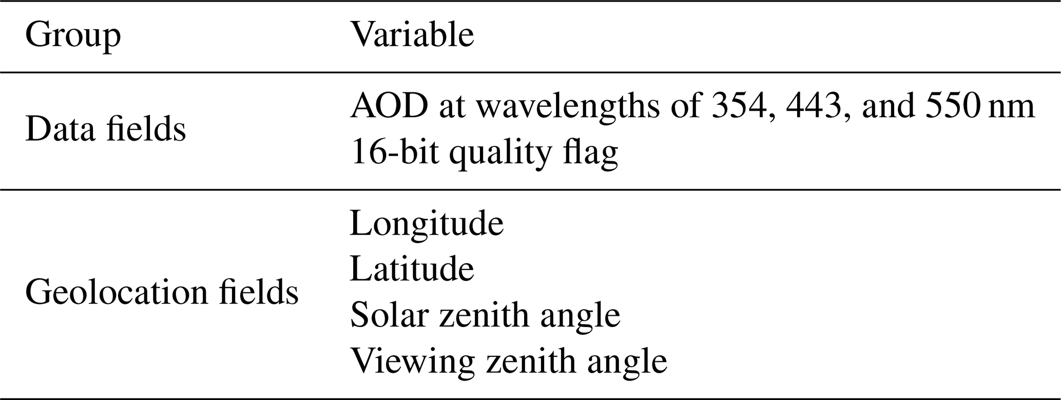
In addition to the solar zenith angle (SZA) and viewing zenith angle (VZA), due to the unavailability of cloud fraction in the GEMS AOD product, we utilize the GEMS L2 cloud product as a masking criterion. The GEMS L2 cloud product is obtained from the GEMS cloud retrieval algorithm (Kim et al., 2024). With the same hyperspectral-measurement range, temporal resolution, and spatial resolution as the GEMS aerosol retrieval algorithm (AERAOD), the GEMS cloud retrieval algorithm retrieves the effective cloud fraction (ECF) and provides the cloud radiance fraction (CRF) via the CRF conversion process (Choi et al., 2024).

To filter out pixels biased toward high cloud fraction, we leverage CRF at wavelengths corresponding to the AOD product.

3 Methodology

We apply a three-stage procedure to calculate the mean field of the L3 AOD products. First, we regrid L2 AOD products using the IDW method with neighboring spatial information to obtain the L3 AOD products. Then, we merge the L3 AOD products by considering spatiotemporal variability in the products, following Kikuchi et al. (2018). Specifically, we merge the L3 AOD products using the previous time T products from the target products of interest. Lastly, we produce the mean field of the L3 AOD products by taking a simple mean of the spatiotemporally merged L3 data. The outline of the method is illustrated in Fig. 1.

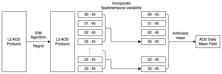
Figure 1 Illustration of the proposed estimation of the mean field methods with a window size of T = 3. All times mentioned in the text are in UTC.

3.1 Inverse distance weighting

In this section, we describe the inverse-distance-weighting (IDW) algorithm used to obtain L3 AOD products. Several methods, including the nearest-neighbor method (Lotrecchiano et al., 2021), the linear interpolation method (Abdullah et al., 2019; Shepard, 1968), and the spline interpolation method (Kuhlmann et al., 2014), have been proposed to interpolate air quality mass. The IDW algorithm (Zimmerman et al., 1999) is one of the most popular linear interpolation methods due to its computational simplicity. Our goal is to obtain the L3 AOD products for each longitude–latitude location.

Let (x₀,y₀) be the target longitude–latitude location for calculating the L3 AOD product. Suppose $(x_{\mathrm{1}},y_{\mathrm{1}}),\mathrm{\dots },(x_n,y_n)$ represent the neighboring longitude–latitude locations of (x₀,y₀), endowed with their corresponding L2 AOD products, denoted by AOD$(x_{\mathrm{1}},y_{\mathrm{1}}),\mathrm{\dots },$ AOD(x_n,y_n). To calculate the L3 AOD product in our application, we use grid points within the fourth-order neighbor of (x₀,y₀). This means that, for the given (x₀,y₀), we use the locations that satisfy $x_i\in (x_{\mathrm{0}}-r,x_{\mathrm{0}}+r)$ and $y_i\in (y_{\mathrm{0}}-r,y_{\mathrm{0}}+r)$. Specifically, we set the resolution to 0.1° for the East Asia region and 0.05° for the Korean Peninsula region. Then, for the fixed observed time point t₀, the IDW estimate is

$$\begin{array}{}\text{(1)}& {\text{AOD}}_{\mathrm{IDW}}(x_{\mathrm{0}},y_{\mathrm{0}},t_{\mathrm{0}})=\sum _i^n{\mathit{\lambda }}_i\text{AOD}(x_i,y_i,t_{\mathrm{0}}),\end{array}$$

where the weight of each location is defined as

$$\begin{array}{}\text{(2)}& {\mathit{\lambda }}_i={\displaystyle \frac{\mathrm{1}/d_i^p}{{\sum }_i^n\mathrm{1}/d_i^p}},\end{array}$$

where d_i is the Euclidean distance from (x₀,y₀) to (x_i,y_i) and p is the power parameter. Therefore, Eq. (1) is based on the weighted average of the L2 AOD values from neighboring locations; a larger weight is assigned to grid points close to the location of interest x₀.

Depending on the choice of p, the IDW estimates yield different outcomes. As p approaches 0, Eq. (2) indicates equal weight, and the IDW estimate approaches a simple average from neighboring locations. On the other hand, as p approaches ∞, the larger weight is concentrated on the locations near x₀, and the IDW estimate converges to the estimate obtained through the nearest neighbor. Although the optimal choice of p can vary depending on the study (Liu et al., 2006), p = 2 is the most commonly used value since when p = 2, the weight for the distance between grid points decays faster to avoid discontinuity (Webster and Oliver, 2007). Following this convention (Isaaks and Srivastava, 1989), we also use p = 2 in our analysis.

Enhanced inverse distance weighting with quality flag information

A quality flag is an indicator that contains data quality information for each grid point. Such indicators are widely used for data cleaning and selection. In our study, we have quality flag information in the L2 AOD products (coded as a 16-bit unsigned integer value). The quality flag used in our study is described in Table 2.

Table 2 Quality flag information. OE: optimal estimation. SFC: surface reflectance. AK: averaging kernel. AMI: Advanced Meteorological Imager.

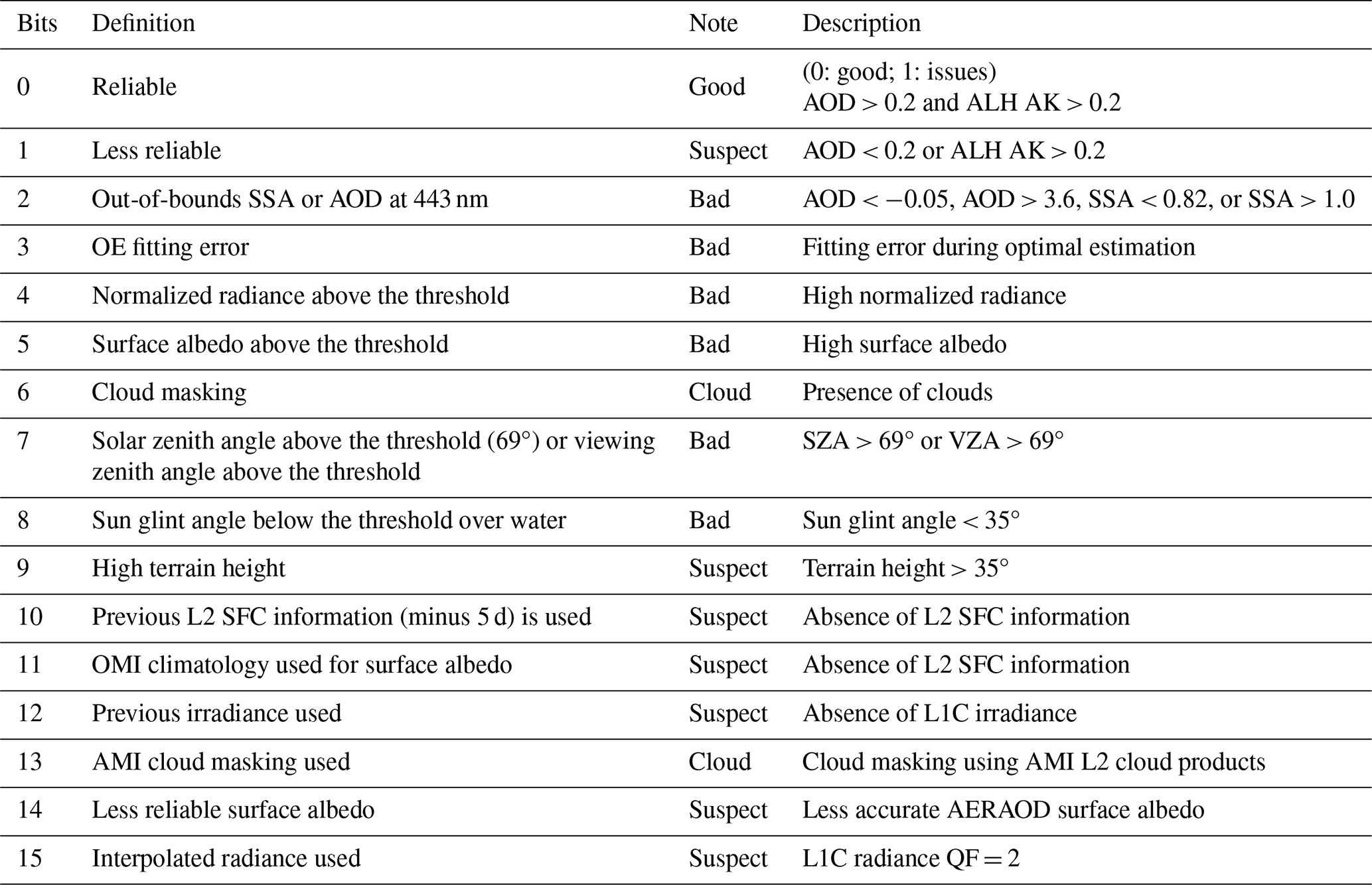
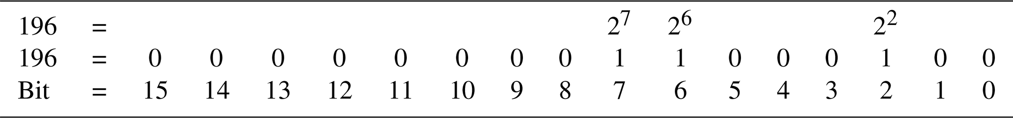
To incorporate quality flag information into the analysis, we convert the 16-bit integer value into a binary value. For instance, the number 196 can be expressed as 000000011000100, which indicates that the features of bit 2, bit 6, and bit 7 are contained. According to Table 2, pixels with an algorithmic quality flag of 196 are likely to have the features of an AOD value smaller than −0.05 or larger than 3.6. In addition, they may have an SSA value smaller than 0.82 or larger than 1.0 in the presence of clouds, when the solar or viewing zenith angle is above the threshold. Table 3 provides further details about the quality flags.

Table 3 Process of converting the number 196, denoting the algorithm quality flag, into 16-bit unsigned integer values and binary values. The first equation shows that the decimal number 196 can be expressed as $\mathrm{196}={\mathrm{2}}^{\mathrm{7}}+{\mathrm{2}}^{\mathrm{6}}+{\mathrm{2}}^{\mathrm{2}}$, which indicates that it can be converted into the binary number 000000011000100 as written in the second line. To show which bits have issues based on the converted binary number, we enumerate bits 0 to 16 on the third line. The process shows that bit 2, bit 6, and bit 7 have issues.

Then, we define an uncertainty metric u_i corresponding to a weight λ_i used in the IDW method. The calculation of the uncertainty metric, denoted as u_i, is based on a quality flag that is represented by a 16-bit unsigned integer. As mentioned, this integer is first converted into a binary format. We then add all the problematic bits with a value of 1 to compute u_i. With this quality flag information, the IDW weight used for our method is expressed as

$$\begin{array}{}\text{(3)}& {\mathit{\lambda }}_i={\displaystyle \frac{\mathrm{1}/d_i^p{u}_i^q}{{\sum }_i\mathrm{1}/d_i^p{u}_i^q}},\end{array}$$

where $u_i=\sum$(bit values of the quality flag) + 1. Since the high values of u_i imply low quality of the data, we take the inverse of u_i in the weights of the IDW algorithm. In Eq. (3), q is a power parameter that controls the amount of quality flag information. The larger the q value, the higher the penalty assigned to the grid with a large u_i value. In Sect. 4, we observe that incorporating quality flags into the weight can improve the accuracy of the IDW method. Furthermore, we validate the choice of quality flags from the simulation study.

3.2 Spatiotemporal merging algorithm

In this section, we describe a merging algorithm (Kikuchi et al., 2018) that can account for spatiotemporal variability in L3 AOD products. Using spatiotemporal information, we can adjust the weights to produce a more robust and accurate L3 AOD mean field output.

3.2.1 Spatiotemporal variability in AOD_IDW

It is crucial to consider the spatiotemporal variability in the IDW estimates when computing the mean field of L3 AOD products (Kikuchi et al., 2018). However, we only have a single IDW estimate, ${\mathbf{AOD}}_{\mathbf{IDW}}(x,y,t)$, at a specific location and time. Since we do not have repeated measures of ${\mathbf{AOD}}_{\mathbf{IDW}}(x,y,t)$, the spatiotemporal variability should be computed using neighboring information. Let $(x_{\mathrm{0}},y_{\mathrm{0}},t_{\mathrm{0}})$ be the location and time of interest and $(x_i,y_i,t_i)$ be the neighboring location i. Then, spatiotemporal variability is defined as a root-mean-square difference (RMSD) of AOD_IDW estimates and is expressed as

$$\begin{array}{}\text{(4)}& \begin{array}{rl}& {\mathit{\sigma }}_{\mathrm{IDW}}(x_{\mathrm{0}},y_{\mathrm{0}},t_{\mathrm{0}})\\ & =\sqrt{{\displaystyle \frac{\mathrm{1}}{N}}\sum _i^N\left({\mathbf{AOD}}_{\mathbf{IDW}}\right(x_i,y_i,t_i)-{\mathbf{AOD}}_{\mathbf{IDW}}(x_{\mathrm{0}},y_{\mathrm{0}},t_{\mathrm{0}}){)}^{\mathrm{2}}},\end{array}\end{array}$$

where N is the number of neighboring pixels within r, which denotes the distance between the point of interest and its neighboring set and previous time T from $(x_{\mathrm{0}},y_{\mathrm{0}},t_{\mathrm{0}})$. In this work, we consider the fourth-order neighboring grids and a window size of T=3, meaning that r = 0.1, 0.2, 0.3, and 0.4° and that t = 0, 1, 2, and 3.

3.2.2 Hourly merged AOD estimates

Using the spatiotemporal variability discussed in Sect. 3.2.1, we compute hourly combined AOD products. The procedure is summarized as follows. First, we obtain AOD_pure by filtering out unreliable grid points. Then, we compute AOD_merged at the location of interest by interpolating AOD_pure. From this, we can retrieve reliable AOD products.

3.2.3 Computing AOD_est

We first introduce ${\mathbf{AOD}}_{\mathbf{est}}(x_{\mathrm{0}},y_{\mathrm{0}},t_{\mathrm{0}})$, which is a weighted average of the IDW estimates obtained in Sect. 3.1. The AOD estimate for a target grid $(x_{\mathrm{0}},y_{\mathrm{0}},t_{\mathrm{0}})$ is given as

$$\begin{array}{}\text{(5)}& {\mathbf{AOD}}_{\mathbf{est}}(x_{\mathrm{0}},y_{\mathrm{0}},t_{\mathrm{0}})=\sum _i^n{w}_i{\mathbf{AOD}}_{\mathbf{IDW}}(x_i,y_i,t_{\mathrm{0}}),\end{array}$$

where

$$\begin{array}{}\text{(6)}& \begin{array}{rl}& w_i={\displaystyle \frac{\frac{\mathrm{1}}{{\mathit{\sigma }}_{\mathrm{IDW}}^{\mathrm{2}}(x_i,y_i,t_{\mathrm{0}})}}{\frac{\mathrm{1}}{{\mathit{\sigma }}_{\mathrm{est}}^{\mathrm{2}}(x_i,y_i,t_{\mathrm{0}})}}}\\ & \text{and}\\ & {\displaystyle \frac{\mathrm{1}}{{\mathit{\sigma }}_{\mathrm{est}}^{\mathrm{2}}(x_{\mathrm{0}},y_{\mathrm{0}},t_{\mathrm{0}})}}=\sum _i^n{\displaystyle \frac{\mathrm{1}}{{\mathit{\sigma }}_{\mathrm{IDW}}^{\mathrm{2}}(x_i,y_i,t_{\mathrm{0}})}}.\end{array}\end{array}$$

Here, n denotes the number of effective pixels within r and past time T from $(x_{\mathrm{0}},y_{\mathrm{0}},t_{\mathrm{0}})$, whose AOD_IDW values are greater than or equal to 0. In Eq. (5), AOD_est is the weighted average of AOD_IDW, and weights are defined by the inverse of the spatiotemporal variability discussed in Sect. 3.2.1. Note that the inverse of the variability quantifies the accuracy and reliability of the IDW estimate for each grid; w_i indicates the sum of the accuracies over the neighboring region of the target point.

3.2.4 Estimating the error variance

Our goal is to filter out grid points with high variability. Note that the spatiotemporal variability in Eq. (4) increases as the distance between grids increases. Utilizing this relationship, we estimate the spatial and temporal variabilities separately through a regression model. The combined variability, denoted as σ₀, for the currently considered grid point $(x_{\mathrm{0}},y_{\mathrm{0}},t_{\mathrm{0}})$ is then calculated as the mean of the spatial and temporal variabilities.

Before estimating the variability, we categorize the values of AOD_IDW into different classes. This is because the pattern of spatiotemporal variability varies depending on the magnitude of the AOD values (Kikuchi et al., 2018). Specifically, we categorize AOD_IDW values into six bins corresponding to 0.1, 0.25, 0.5, 0.75, 0.9, and 1.0. Note that previous work (Kikuchi et al., 2018) used 12 classes. However, we use six classes because certain classes are rarely observed; using 12 classes can lead to unreliable computation.

Let ${\mathit{\sigma }}_{\mathrm{dist}}(x_{\mathrm{0}},y_{\mathrm{0}},t_{\mathrm{0}})$ be the spatial variability and ${\mathit{\sigma }}_{\mathrm{time}}(x_{\mathrm{0}},y_{\mathrm{0}},t_{\mathrm{0}})$ be the temporal variability in the IDW estimate at $(x_{\mathrm{0}},y_{\mathrm{0}},t_{\mathrm{0}})$. We first compute the average of the spatiotemporal variability ${\mathit{\sigma }}_{\mathrm{IDW}}(x_i,y_i,t_i)$ based on r and the class. Then, we regress the averaged values obtained for each component of the vector r = (0.1°, 0.2°, 0.3°, 0.4°) on a design matrix $[\mathbf{1},\mathit{r},{\mathit{r}}^{\mathbf{2}}]$, which is a second-order design matrix for r pertaining to each class. Lastly, we obtain the spatial variability ${\mathit{\sigma }}_{\mathrm{dist}}(x_{\mathrm{0}},y_{\mathrm{0}},t_{\mathrm{0}})$ from the intercept estimate of the quadratic regression model fitting. We can obtain the temporal variability ${\mathit{\sigma }}_{\mathrm{time}}(x_{\mathrm{0}},y_{\mathrm{0}},t_{\mathrm{0}})$ in a similar manner. We first compute the average of the spatiotemporal variability ${\mathit{\sigma }}_{\mathrm{IDW}}(x_i,y_i,t_i)$ based on the time point and class. We regress them on a design matrix $[\mathbf{1},\mathit{t},{\mathit{t}}^{\mathbf{2}}]$ for each class and obtain ${\mathit{\sigma }}_{\mathrm{time}}(x_{\mathrm{0}},y_{\mathrm{0}},t_{\mathrm{0}})$ from the intercept estimate of the quadratic regression model fitting.

Finally, we compute the error variance by taking the average of σ_dist and σ_time, given as

$$\begin{array}{}\text{(7)}& {\mathit{\sigma }}_{\mathrm{0}}(x_{\mathrm{0}},y_{\mathrm{0}},t_{\mathrm{0}})={\displaystyle \frac{{\mathit{\sigma }}_{\mathrm{dist}}(x_{\mathrm{0}},y_{\mathrm{0}},t_{\mathrm{0}})+{\mathit{\sigma }}_{\mathrm{time}}(x_{\mathrm{0}},y_{\mathrm{0}},t_{\mathrm{0}})}{\mathrm{2}}}.\end{array}$$

The calculated error variance contains a measurement error caused by sensor noise that varies over time and space.

3.2.5 Computing AOD_pure

Here, we obtain AOD_pure by filtering out uncertain AOD_IDW values. For this, we introduce the estimated error in AOD_pure, which is defined as

$$\begin{array}{rl}& {\mathit{\sigma }}_{\mathrm{pure}}(x_{\mathrm{0}},y_{\mathrm{0}},t_{\mathrm{0}})\\ & =\left\{\begin{array}{l}\begin{array}{rl}& \sqrt{{\mathit{\sigma }}_{\mathrm{0}}^{\mathrm{2}}(x_{\mathrm{0}},y_{\mathrm{0}},t_{\mathrm{0}})+{\mathit{\sigma }}_{\mathrm{est}}^{\mathrm{2}}(x_{\mathrm{0}},y_{\mathrm{0}},t_{\mathrm{0}})},\\ & \text{if}{\mathbf{AOD}}_{\mathbf{IDW}}(x_{\mathrm{0}},y_{\mathrm{0}},t_{\mathrm{0}})\text{is observed},\end{array}\\ \text{missing},\text{otherwise}.\end{array}\right.\end{array}$$

Here, ${\mathit{\sigma }}_{\mathrm{est}}^{\mathrm{2}}$ is the error variance of AOD_est from Eq. (6) and ${\mathit{\sigma }}_{\mathrm{0}}^{\mathrm{2}}$ is the combined error variance from Eq. (7). To filter out uncertain AOD_IDW values, we consider an upper threshold of AOD_IDW, expressed as

$$\begin{array}{}\text{(8)}& \begin{array}{rl}& {\mathbf{AOD}}_{\mathrm{pure}}(x_{\mathrm{0}},y_{\mathrm{0}},t_{\mathrm{0}})\\ & =\left\{\begin{array}{l}\begin{array}{rl}& {\mathbf{AOD}}_{\mathbf{IDW}}(x_{\mathrm{0}},y_{\mathrm{0}},t_{\mathrm{0}}),\text{if}{\mathbf{AOD}}_{\mathbf{IDW}}(x_{\mathrm{0}},y_{\mathrm{0}},t_{\mathrm{0}})\\ & \le {\mathbf{AOD}}_{\mathbf{est}}(x_{\mathrm{0}},y_{\mathrm{0}},t_{\mathrm{0}})+\mathrm{2.58}{\mathit{\sigma }}_{\mathrm{pure}}(x_{\mathrm{0}},y_{\mathrm{0}},t_{\mathrm{0}}),\end{array}\\ \text{missing},\text{otherwise}.\end{array}\right.\end{array}\end{array}$$

Assuming a Gaussian distribution, if ${\mathbf{AOD}}_{\mathbf{IDW}}(x_{\mathrm{0}},y_{\mathrm{0}},t_{\mathrm{0}})$ exceeds the upper threshold of the 99 % confidence interval, we consider the value to be unreliable and thus exclude it from the mean field calculation.

3.2.6 Computing AOD_merged

Based on Sect. 3.2.5, we calculate the total variability within the neighboring grids of the target grid. Then, we use the ratio of the inverse of this total variability to assign weights for calculating a weighted average of AOD_pure, resulting in AOD_merged, given as follows:

$$\begin{array}{}\text{(9)}& \begin{array}{rl}& {\text{AOD}}_{\mathrm{merged}}(x_{\mathrm{0}},y_{\mathrm{0}},t_{\mathrm{0}})\\ & =\left\{\begin{array}{l}\begin{array}{rl}& \sum _i^n{w}_i{\mathbf{AOD}}_{\mathrm{pure}}(x_i,y_i,t_{\mathrm{0}}),\\ & \text{if}{\mathbf{AOD}}_{\mathrm{IDW}}(x_{\mathrm{0}},y_{\mathrm{0}},t_{\mathrm{0}})\text{is observed},\end{array}\\ \text{missing},\text{otherwise},\end{array}\right.\end{array}\end{array}$$

where

$$\begin{array}{rl}& w_i={\displaystyle \frac{\frac{\mathrm{1}}{{\mathit{\sigma }}_{\mathrm{pure}}^{\mathrm{2}}(x_i,y_i,t_{\mathrm{0}})}}{\frac{\mathrm{1}}{{\mathit{\sigma }}_{\mathrm{merged}}^{\mathrm{2}}(x_{\mathrm{0}},y_{\mathrm{0}},t_{\mathrm{0}})}}}\\ & \text{and}\\ & {\displaystyle \frac{\mathrm{1}}{{\mathit{\sigma }}_{\mathrm{merged}}^{\mathrm{2}}(x_{\mathrm{0}},y_{\mathrm{0}},t_{\mathrm{0}})}}=\sum _i^n{\displaystyle \frac{\mathrm{1}}{{\mathit{\sigma }}_{\mathrm{pure}}^{\mathrm{2}}(x_i,y_i,t_{\mathrm{0}})}}.\end{array}$$

This merging process not only utilizes the reliable value (AOD_pure) but also incorporates the reliability (σ_pure) as a weight, resulting in a more trustworthy gap-filling outcome. In fact, in the study by Kikuchi et al. (2018), the root mean squared error (RMSE) of AOD_merged was notably lower (0.11) compared to the RMSE of AOD_IDW (0.20).

4 Simulation

In this section, we conduct a simulation study to validate the choice of quality flags. The data generation procedure is summarized as follows.

4.1 Generating simulation data

1. For our simulation study, we constructed a 70 × 70 lattice over a 1 × 1 square domain with a grid spacing of 0.1°. Each grid within this lattice represents a location in our simulated dataset. In total, the lattice comprises 4900 grid cells, covering an area of 7° × 7°. Consequently, each unit grid on the lattice represents an area of 0.1° × 0.1°. We generate each element of $\mathbf{X}\in {\mathbb{R}}^{\mathrm{4900}\times \mathrm{2}}$ from Unif(0,1), i.e., uniform distribution with support from 0 to 1. This means that we have 4900 locations, each containing two pieces of coordinate information: longitude and latitude. We use ${\mathit{\beta }}_{\mathrm{1}\times \mathrm{2}}=(\mathrm{1},\mathrm{1})$ as a true coefficient vector.

2. For each location, we simulate a zero-mean Gaussian process W from $N(\mathrm{0},(\mathit{\tau }{\mathbf{M}}^{\prime }\mathbf{\text{QM}}{)}^{-\mathrm{1}})$, where M is obtained by taking the first k eigenvectors of the Moran operator (Hughes and Haran, 2013) using smoothness parameter τ. Here, Q = diag(A1) − A is a precision matrix calculated from the adjacency matrix A. Note that 1 is an all-ones vector.

3. We simulate AOD datasets from $\mathbf{Y}=\mathbf{X}\mathit{\beta }+\mathbf{W}\in {\mathbb{R}}^{\mathrm{4900}\times \mathrm{2}}$. In our simulation, Xβ represents the fixed effect, while W∈ℝ⁴⁹⁰⁰ accounts for spatial correlation in AOD products.

4. To generate missing data for the simulated Y that resemble the GEMS L2 product, we apply the observed missing pattern from the GEMS AOD data to the simulated Y from step 3. Specifically, we apply the missing data pattern observed in the GEMS AOD data for the 7° × 7° region in East Asia, with a grid spacing of 0.1°, collected on 1 April at 04:45 UTC. This selected dataset aligns with the 70 × 70 lattice in our simulation and has approximately 20 % of its values missing, effectively replicating the realistic missing data characteristics found in the actual GEMS AOD observations.

5. For a realistic simulation that incorporates the physical implications of quality flags, we adapt the observed quality flags from the GEMS AOD data to the simulated Y from step 3. Similar to step 4, we use the quality flag from the same data (i.e., data from the 7° × 7° region in East Asia (with a grid spacing of 0.1°), collected on 1 April at 04:45 UTC) for the simulated Y.

We repeat steps 1–3 100 times to generate different realizations of Y. Then, for each simulated Y, we apply the identical missing patterns (step 4) and quality flags (step 5) obtained from the real dataset. Figure 2 illustrates an example of a simulated dataset.

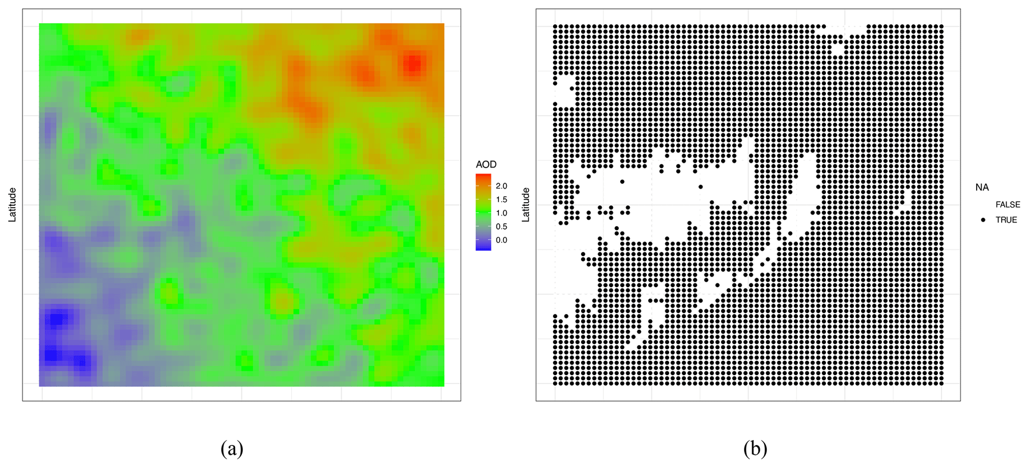
Figure 2 Panel (a) illustrates the simulated AOD dataset, and panel (b) shows the missing pattern (white color). Panel (a) shows the simulated AOD values, while panel (b) shows the missing patterns.

4.2 Sensitivity analysis of q

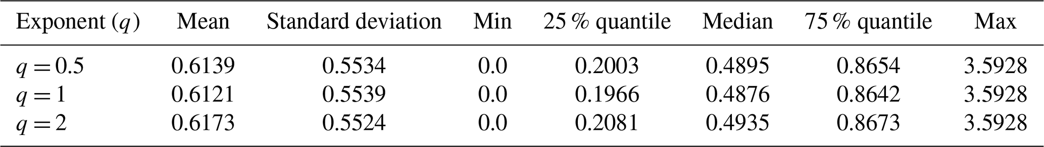
Here, we investigate the performance of the IDW method with regard to GEMS data by varying q in Eq. (3). Specifically, we consider q values of 0.5, 1, and 1.5 in our experiment. We first examine whether there is a significant difference in IDW estimates with difference choices of q. Figure 3 indicates that the IDW estimates are comparable with various q values. Table 4 also shows that the summary statistics of AOD_IDW are quantitatively similar across different q choices. Therefore, we conclude that the IDW algorithm is robust regardless of the q value used. To simplify the calculation, we set q = 1 in our analysis.

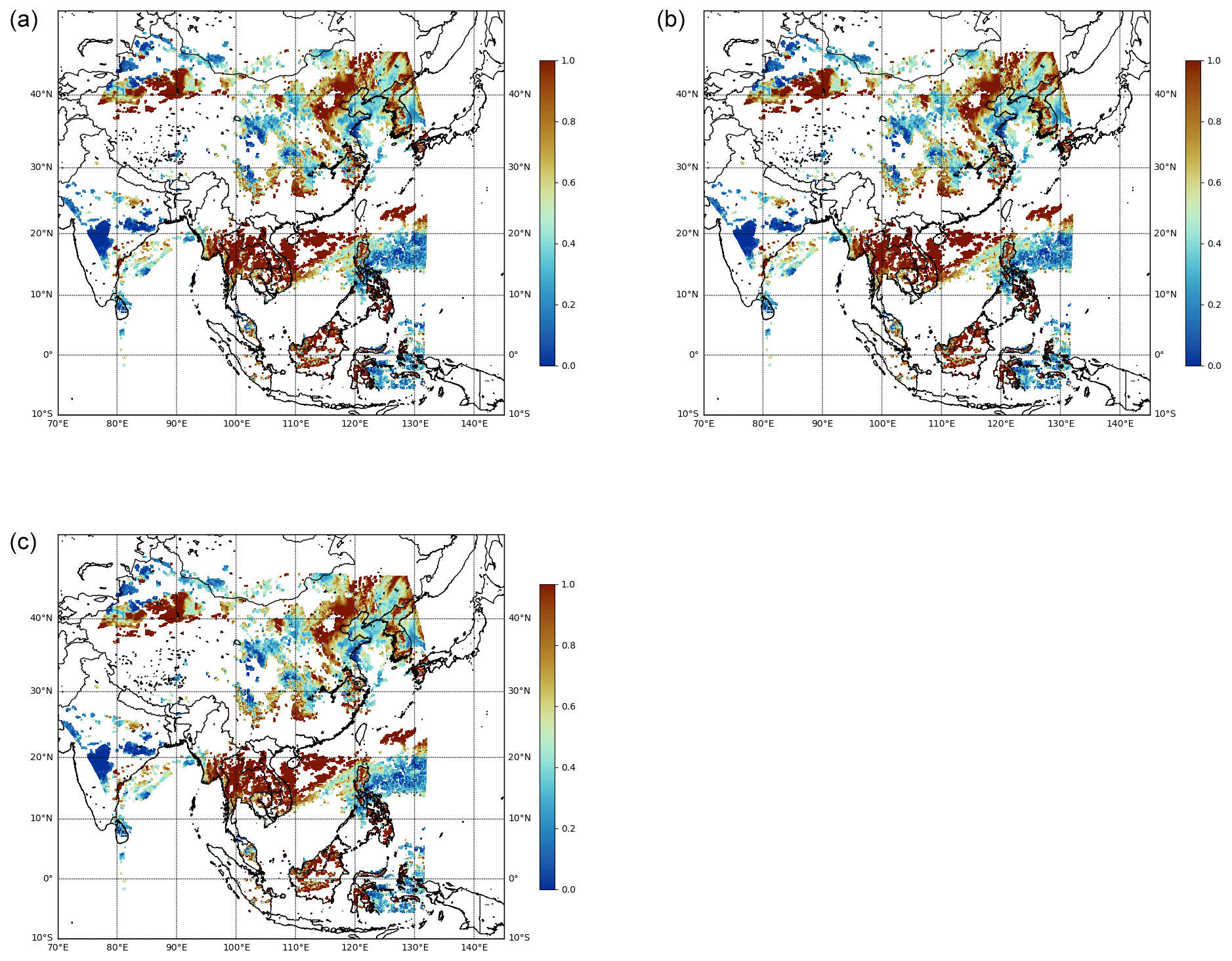
Figure 3 Comparison of the IDW estimates obtained on 1 April 2023 at 07:00 UTC. Each panel illustrates AOD_IDW with q = 0.5 (a), q = 1 (b), and q = 2 (c).

Table 4 Summary statistics of AOD_IDW values for different q values obtained on 1 April 2023 at 07:00 UTC.

4.3 Quality flag simulation

As explained in Sect. 4.2 and Eq. (3), quality flag indicators weigh the uncertainty in the IDW algorithm. To improve the accuracy of the IDW algorithm, it is necessary to find the optimal bit combination of the quality flag by performing simulation studies. Therefore, we first identify bits that show substantially lower mean squared errors (MSEs) and then combine these specific bits into groups. Here, the MSE is calculated between the simulated AOD dataset and the IDW results, given by

$${\displaystyle \frac{\mathrm{1}}{n}}\sum _{i=\mathrm{1}}^n{\left({\text{AOD}}_i-{\text{IDW}}_i\right)}^{\mathrm{2}},$$

where AOD_i is the simulated AOD value at location i and IDW_i is the IDW result at location i. Note that we refer to these bit combinations of quality flags as “cases”. For example, we may find that bits 0, 1, and 2 have a significantly low MSE. This means that we can create various combinations of these bits, such as 0 ⋅ 1, 0 ⋅ 2, or even 0 ⋅ 1 ⋅ 2, and each combination can be denoted as a particular “case”.

Before finding the optimal case of the quality flag through a simulation study, we examine whether the result differs depending on the value of r in the IDW algorithm. Note that this simulation study defines the unit of r as one unit grid and not as the distance based on coordinates, as described in Sect. 3.1. After careful consideration and analysis, we have chosen to set the neighboring order to 3 for our study because varying the order of the neighbors did not yield any significant differences in the mean squared error (MSE). However, to provide a comprehensive understanding of the impact of the order on the interpolation process, we have included additional IDW results with increasing order sizes in Appendix A. These supplementary results demonstrate that larger order sizes can potentially lead to oversmoothing. Figure 4 shows the generated AOD simulation data, with panel (b) indicating the data incorporating the missing value pattern and panel (b) visualizing the result of applying the IDW algorithm to the data.

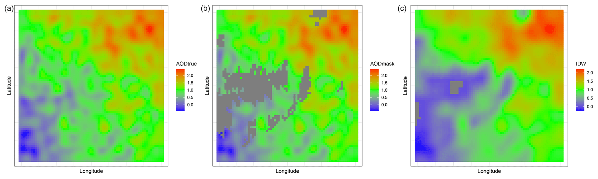
Figure 4 Panel (a) shows the simulated AOD values, while panel (b) shows the simulated data incorporating the missing pattern, indicated by the gray color. Panel (c) illustrates the result of applying the IDW algorithm to simulated data when r = 3.

We then follow the following procedure. After selecting specific bits with a lower MSE than bits fixed with an order of 3, we repeat the experiment to account for diverse uncertainty term calculations by considering various cases in the IDW algorithm. We then find the optimal case that obtains the highest accuracy by comparing the accuracies among the cases. Here, MSE values are evaluated between the simulation and the imputed data, treating the simulated data as real data.

To select the quality flag bit for making the combination case, we first calculate the MSE for each quality flag bit. Figure 5 displays the MSE values as boxplots for each bit. Although the boxplots indicate the results for bits 0 through 15, bit 2 and bit 6 exhibit significantly lower MSEs than other bits. The medians for the two bits are 0.122 and 0.123, respectively. Bit 2 indicates whether SSA or AOD is outside a specific value range, while bit 6 shows the presence of clouds. We then compile six different candidate cases, including bit 2 and bit 6. Table 5 summarizes these six candidate cases.

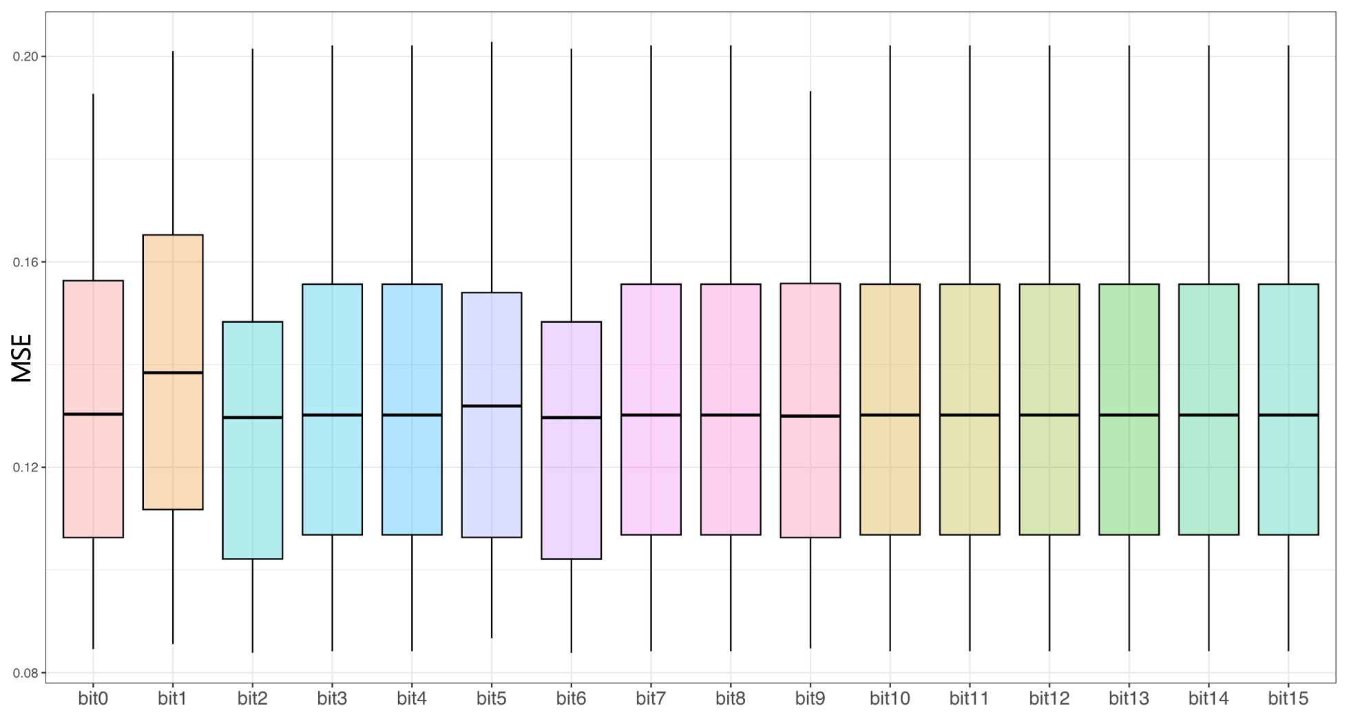
Figure 5 Boxplots illustrating the interquartile ranges of the IDW algorithm results from 100 repetitive simulation datasets, including bits 0 through 15, for the uncertainty metric σ(i). The boxes represent the interquartile ranges, extending from the first quartile (Q1) to the third quartile (Q3), with a horizontal line inside each boxplot denoting the median of the repeated simulations. The boundary of the lower whisker represents the minimum value of the MSE. In contrast, the boundary of the upper whisker represents the maximum value of the MSE across the repeated simulations. We find that bit 2 and bit 6 have a lower MSE than other bits.

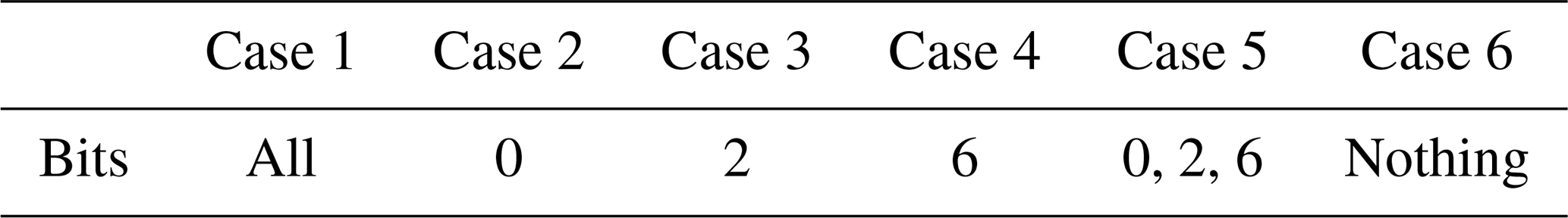
Table 5 Six candidate cases for selecting quality flags based on the combinations of bits 0, 2, and 6.

To find the optimal quality control case that yields the lowest MSE among the six candidate cases, we calculate the MSE for each case using two different τ values, τ = 1 and τ = 6, and present boxplots in Fig. 6. In Fig. 6a and b, each case shows a different MSE, while case 5, which contains bits 0, 2, and 6, shows the lowest median (0.387) in Fig. 6a. Therefore, for our real application, we use the quality flag for case 5 (bits 0, 2, and 6) when calculating the uncertainty term for the IDW algorithm.

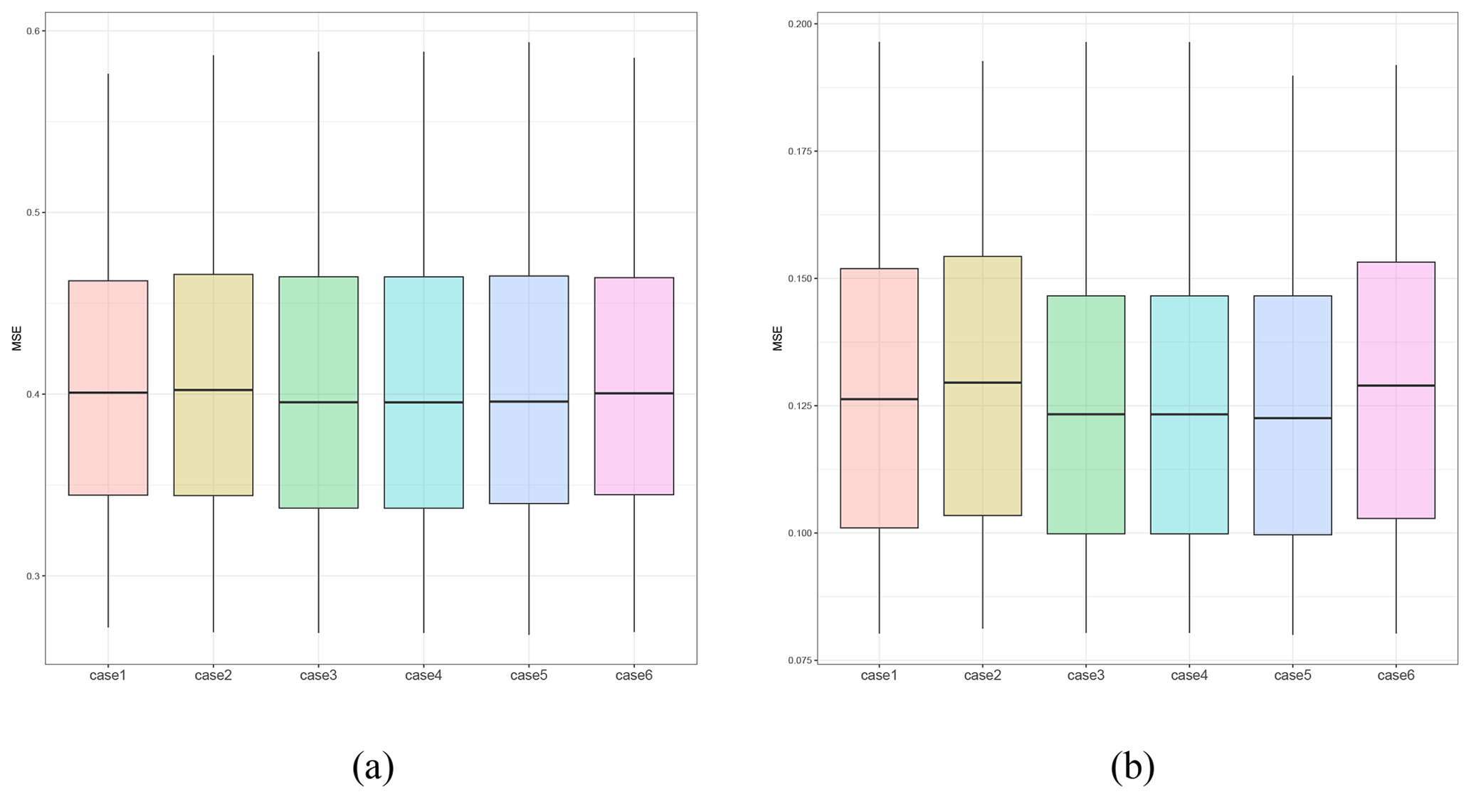
Figure 6 Panel (a) shows the simulation results when τ = 1, while panel (b) shows the results when τ = 6. Despite the value of the smoothing parameter τ, we find that the hierarchy of the MSE values between the cases is identical.

We examine whether the optimal case for the IDW algorithm changes depending on the smoothing parameter τ of the simulation data. Figure 6a and b show the average MSE, represented as boxplots, with different smoothing parameters. We find that while the overall magnitude of the MSE value differs, the hierarchy of the MSEs across the cases remains unchanged. This suggests that the algorithm's performance is robust regardless of the smoothing parameter used.

5 GEMS data application

5.1 Spatial resolution of output product

A geostationary satellite instrument, such as the GEMS, observes a fixed position. Therefore, if we use grids that are too small, the output will have many missing values; an appropriate grid size should be selected to ensure adequate coverage of the mean fields. Furthermore, we need to consider the effective range, accuracy, and computation time needed to obtain mean fields when choosing a grid size. If we use too fine a spatial resolution, computational costs will exponentially increase. On the other hand, grid sizes that are too large can lead to inaccurate output results. Accordingly, in our study, we set the mean field spatial resolution of the longitude–latitude grid to 0.1° × 0.1° and 0.05° × 0.05° for the East Asia and Korean Peninsula regions, respectively.

5.2 Level-2 aerosol optical depth data

As evidenced by various studies (Kaufman et al., 2005; Loeb and Manalo-Smith, 2005; Matheson et al., 2005), AOD exhibits a positive correlation with cloud fraction (CF), implying that proximity to clouds can result in a statistical increase in AOD measurements. Additionally, a dependency of AOD on solar and viewing zenith angles was observed (de Miguel et al., 2011), highlighting the complexities involved in accurate AOD estimation under varied atmospheric conditions. To address these complexities, this study involved masking data based on three variables, given below. Cloud radiance fraction is incorporated within the GEMS L2 cloud product, while the others are incorporated within the GEMS L2 AOD product. These variables are meticulously designed to account for variability and uncertainties in satellite data (Choi et al., 2024), addressing factors such as solar and viewing zenith angles and cloud radiance fraction. This methodology ensures a more precise and reliable estimation of AOD, which is crucial for understanding atmospheric dynamics and environmental monitoring. Unreliable values are treated as missing values when we apply the IDW algorithm. The thresholds are as follows:

• cloud radiance fraction ≥ 0.4

• solar zenith angle ≥ 70°

• viewing zenith angle ≥ 70°.

In our study, we set two spatial domains for the mean field outputs – one with latitude (30–43° N) and longitude (123–131° E) corresponding to the vicinity of the Korean Peninsula and the other with latitude (32–43° N) and longitude (115–131° E) including the vicinity of the Shandong Peninsula in China.

5.3 Mean field estimates of the GEMS L3 AOD product

Figures 7 and 8 compare the spatiotemporally merged products with the simply averaged products. For spatiotemporally merged L3 AOD products, we apply the procedure described in Sect. 3. On the other hand, we take the mean of the IDW estimates for simply averaged L3 AOD products. As mentioned in Kikuchi et al. (2018), grid points with AOD values exceeding 1.0 are extremely rare. Therefore, to focus on the majority of values for detailed characterization, we set the threshold to 1.0. In Fig. 7, we observe that more missing values occur in the area of latitude (20–30° N) and longitude (130–140° E) for the spatiotemporally merged products compared to that for the simply averaged products. This can also be verified by the ratio of missing values for each product shown in each figure. This is due to the fact that a spatiotemporal merging procedure only considers reliable AOD estimates, while a simple averaging method does not. Therefore, the simply averaged products can be regarded as more unreliable, although they have fewer missing values. In Fig. 7, we also observe that the spatiotemporal merging method can provide smoother mean field outputs; for example, there is a significant difference in the area of latitude (35–45° N) and longitude (125–135° E). Similar trends are also observed in Fig. 8. Mean field estimates at all three wavelengths for the East Asia and the Korean Peninsula regions are provided in Appendix B and C, respectively.

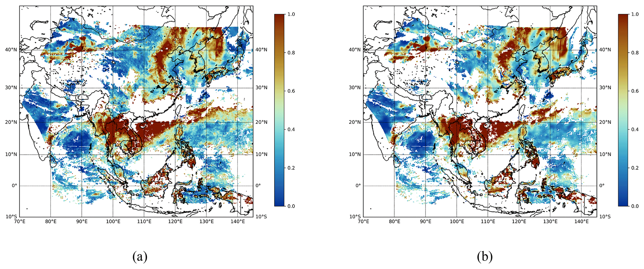
Figure 7 Daily mean field estimates of the GEMS L3 AOD product obtained on 1 April 2023 at a wavelength of 354 nm. (a) Simply averaged output. (b) Spatiotemporally merged output. The missing ratio for panel (a) is 0.5031, and the missing ratio for panel (b) is 0.5733.

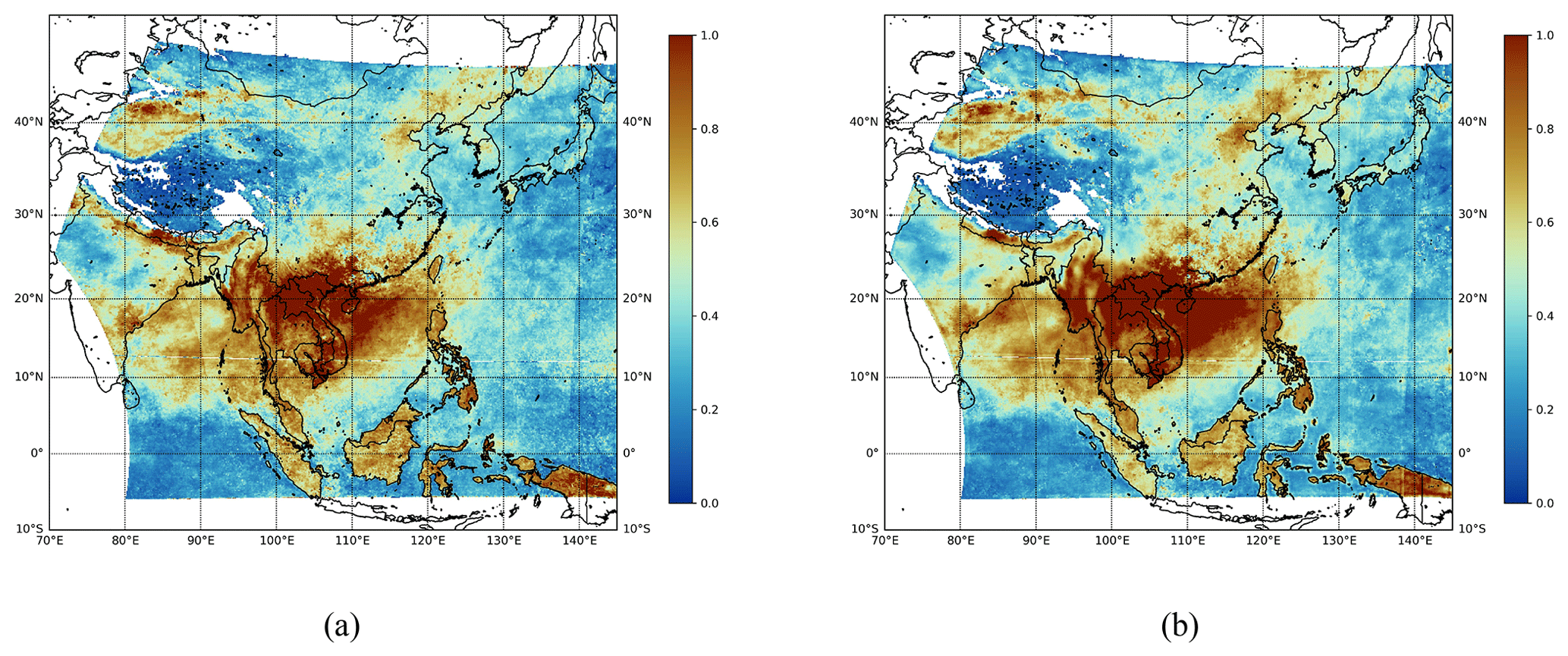
Figure 8 Monthly mean field estimates of the GEMS L3 AOD product obtained on April 2023 at a wavelength of 354 nm. (a) Simply averaged output. (b) Spatiotemporally merged output. The missing ratio for panel (a) is 0.1485, and the missing ratio for panel (b) is 0.1489.

As described in Sect. 3, we obtain AOD_pure from AOD_est by considering both the spatiotemporal variability σ₀ and the estimation uncertainty σ_est. This procedure allows us to obtain more reliable AOD estimates. Furthermore, we can use more robust AOD estimates when computing the mean field, resulting in a smoother output.

5.4 Qualitative evaluation of the mean field products

Directly evaluating the accuracy of the L3 AOD mean field products is challenging because there are no true values for these products. Therefore, we compare our results with previous studies using qualitative aspects.

In Fig. 9a, we observe that our mean field products obtained at a 550 nm wavelength on 1 April are similar to the springtime global distribution of AOD at the same wavelength. Furthermore, high values due to dust are observed near the Taklamakan Desert, and high values due to biomass burning are observed in Southeast Asia during spring. This indicates that the computed mean fields can effectively capture real-world phenomena. In addition, we observe that the overall trends in AOD values are similar to those from Moderate Resolution Imaging Spectroradiometer (MODIS) data (Tian et al., 2023), although there are some discrepancies among values pertaining to the vicinity of the Taklamakan Desert and certain areas in Southeast Asia.

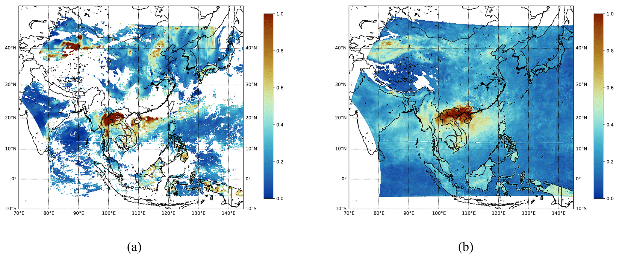
Figure 9 Mean field estimates of the GEMS L3 AOD product obtained in April 2023 at a wavelength of 550 nm. (a) Daily mean field output for 1 April 2023. (b) Monthly mean field output for April 2023.

5.5 Quantitative evaluation of the mean field products

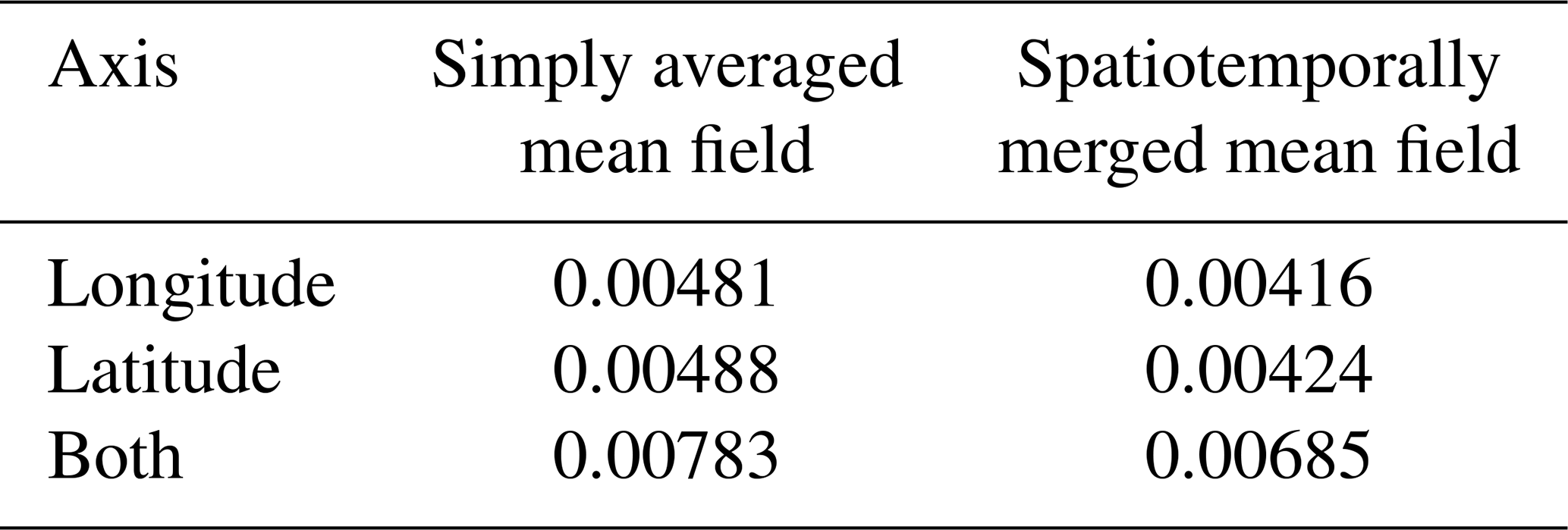
To measure the smoothness of the mean field products, we compute the second-order gradients of the AOD estimates from the longitude and latitude. Specifically, we compute gradients at each pixel point based on its neighboring AOD values, following previous studies (Fornberg, 1988; Quarteroni et al., 2007; Durran, 1999). Then, we compare the absolute mean of the gradients from the simple and spatiotemporal averaging methods. Table 6 indicates that gradients in both directions are smaller in the spatiotemporal merging method. Considering that AOD exhibits significant spatiotemporal variability, our method provides more realistic mean field products than the simple averaging method.

Table 6 Comparison of gradients between merging algorithms.

6 Conclusions

In remote sensing, data are processed according to different levels. For example, the L2 dataset, which contains atmospheric-state retrievals, is converted into the L3 dataset. Specifically, we focus on AOD retrievals from the GEMS instrument through gap filling and noise filtering. We improve the quality of L3 AOD mean field products by considering quality flag information and spatiotemporal variability (Kikuchi et al., 2018). Specifically, the contribution of our work is summarized as follows.

First, we improve the performance of the IDW algorithm by including quality flag information in the weight calculation. We assign weights that are inversely proportional to the number of poor-quality indicators. To validate the choice of different quality flags, we conduct simulation studies. We observe that including bits 0, 2, and 6 from the quality flags significantly improves the accuracy of the IDW algorithm. We apply this novel approach to GEMS AOD data covering various regions and wavelengths.

Second, we apply a spatiotemporal merging method (Kikuchi et al., 2018) to GEMS AOD data. Unlike previous work (Park et al., 2023) that only considered spatial variability, our method also accounts for temporal variability from previous time points. We observe that our mean field products exhibit similar trends to the previous studies, indicating that the products are reliable.

Although our current study has made notable progress in enhancing the accuracy of AOD mean field estimation, several avenues for future research remain. One potential direction involves integrating additional data, such as cloud information and distinctions between oceanic and terrestrial regions, to further refine our results by considering the impact of cloud cover on aerosol retrievals. Our method can account for variability due to cloud contamination by utilizing quality flag information in the IDW estimates. Note that we cannot use physical mechanisms (e.g., aerosols produced by wildfires) in the interpolation step due to limited data sources. Developing extensions of our approach by incorporating physical mechanisms may provide interesting future research avenues. Additionally, with the available information on quality flags, one direction for future work could involve developing methodologies for adaptively weighting or selecting quality flag bits by employing statistical variable selection methodologies. Validating our AOD mean field products against ground-based measurements or other satellite datasets could also offer valuable insights into their reliability and consistency, thereby helping to identify any potential biases or uncertainties. Lastly, conducting a sensitivity analysis to choose hyperparameters (e.g., the order of neighboring grids and time windows) would be useful for improving the performance of the method.

Appendix A: Sensitivity analysis for the radius of the IDW algorithm

We compare the results of applying the IDW algorithm with varying orders of neighboring grids used for a weighted average. Observing the visualization, we find a remarkable difference in the imputed area as fewer missing values remain with an order of 9 compared to an order of 3. However, the MSE values are 0.255 and 0.25, respectively, showing no significant difference in numbers. Despite the negligible difference between the two window sizes, we determined that the window size should be 3 since an order of 9 could cause oversmoothing.

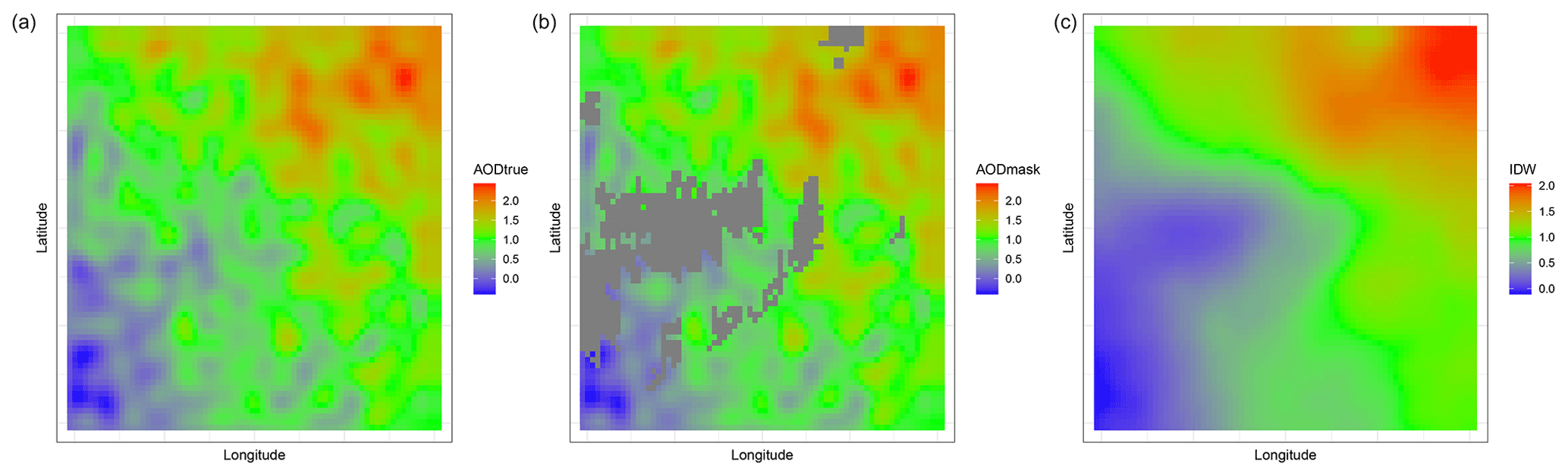
Figure A1 Panel (a) shows the simulated AOD values, while panel (b) shows the simulated data incorporating the missing pattern, indicated by the gray color. Panel (c) illustrates the result of applying the IDW algorithm to the simulated data with an order of 9.

Appendix B: Mean field estimates of the GEMS L3 AOD product for East Asia

In this section, we include daily and monthly mean field estimates of the GEMS L3 AOD products at all three wavelengths for East Asia.

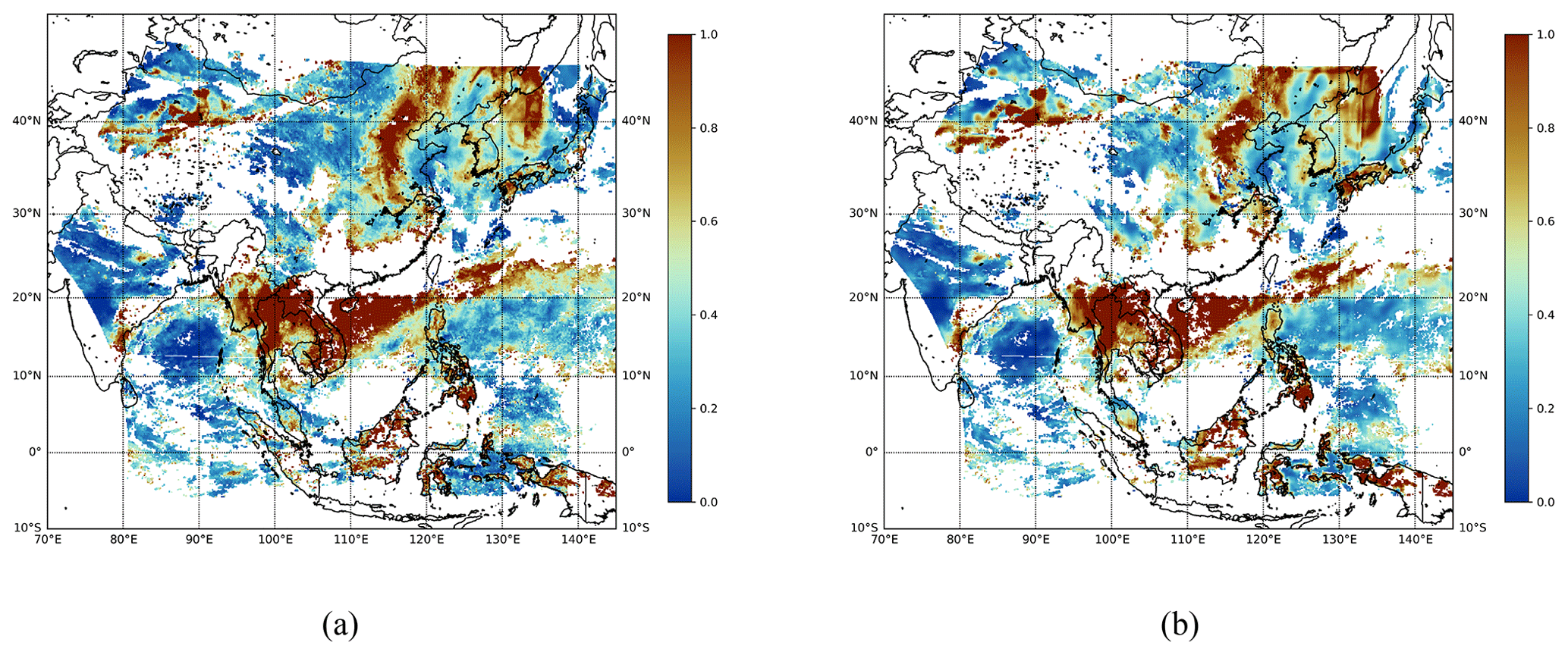
Figure B1 Daily mean field estimates of the GEMS L3 AOD product obtained on 1 April 2023 at a wavelength of 354 nm. (a) Simply averaged output. (b) Spatiotemporally merged output. The missing ratio for panel (a) is 0.5031, and the missing ratio for panel (b) is 0.5733.

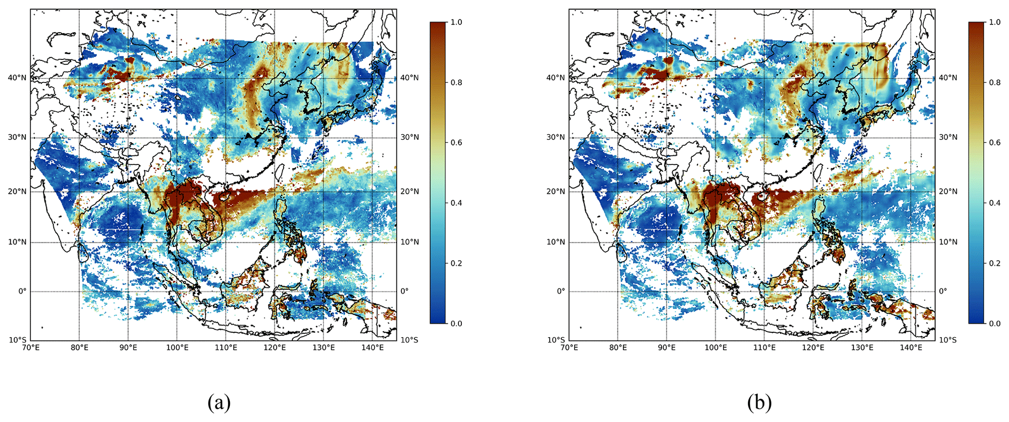
Figure B2 Daily mean field estimates of the GEMS L3 AOD product obtained on 1 April 2023 at a wavelength of 443 nm. (a) Simply averaged output. (b) Spatiotemporally merged output. The missing ratio for panel (a) is 0.5000, and the missing ratio for panel (b) is 0.5710.

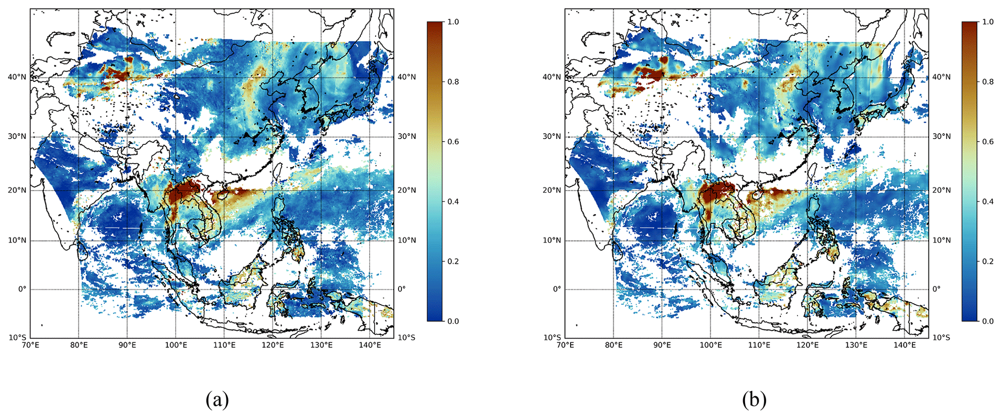
Figure B3 Daily mean field estimates of the GEMS L3 AOD product obtained on 1 April 2023 at a wavelength of 550 nm. (a) Simply averaged output. (b) Spatiotemporally merged output. The missing ratio for panel (a) is 0.4908, and the missing ratio for panel (b) is 0.5619.

Figure B4 Monthly mean field estimates of the GEMS L3 AOD product obtained in 1 April 2023 at a wavelength of 354 nm. (a) Simply averaged output. (b) Spatiotemporally merged output. The missing ratio for panel (a) is 0.1485, and the missing ratio for panel (b) is 0.1489.

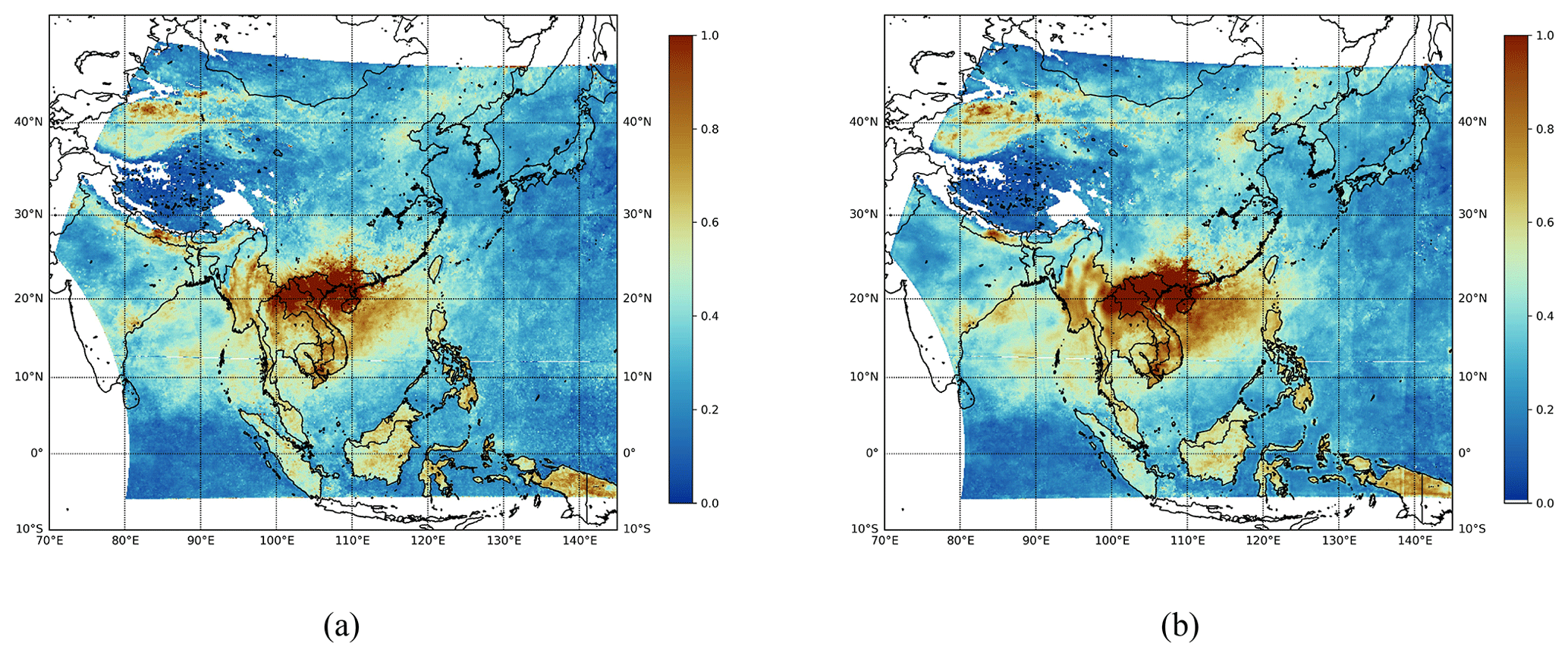
Figure B5 Monthly mean field estimates of the GEMS L3 AOD product obtained in April 2023 at a wavelength of 443 nm. (a) Simply averaged output. (b) Spatiotemporally merged output. The missing ratio for panel (a) is 0.1490, and the missing ratio for panel (b) is 0.1494.

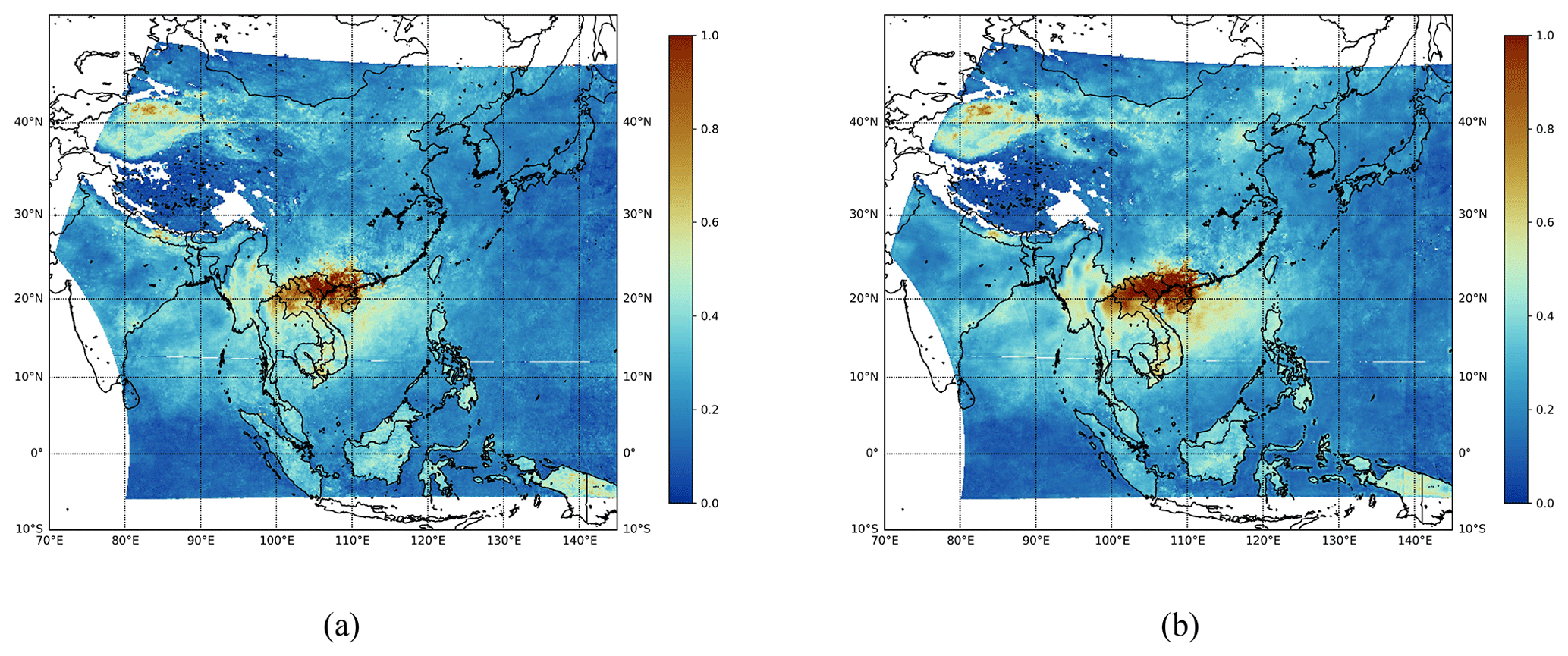
Figure B6 Monthly mean field estimates of the GEMS L3 AOD product obtained in April 2023 at a wavelength of 550 nm. (a) Simply averaged output. (b) Spatiotemporally merged output. The missing ratio for panel (a) is 0.1483, and the missing ratio for panel (b) is 0.1487.

Appendix C: Mean field estimates of the GEMS L3 AOD product for the Korean Peninsula region

In this section, we include daily and monthly mean field estimates of the GEMS L3 AOD products at three wavelengths for the Korean Peninsula region.

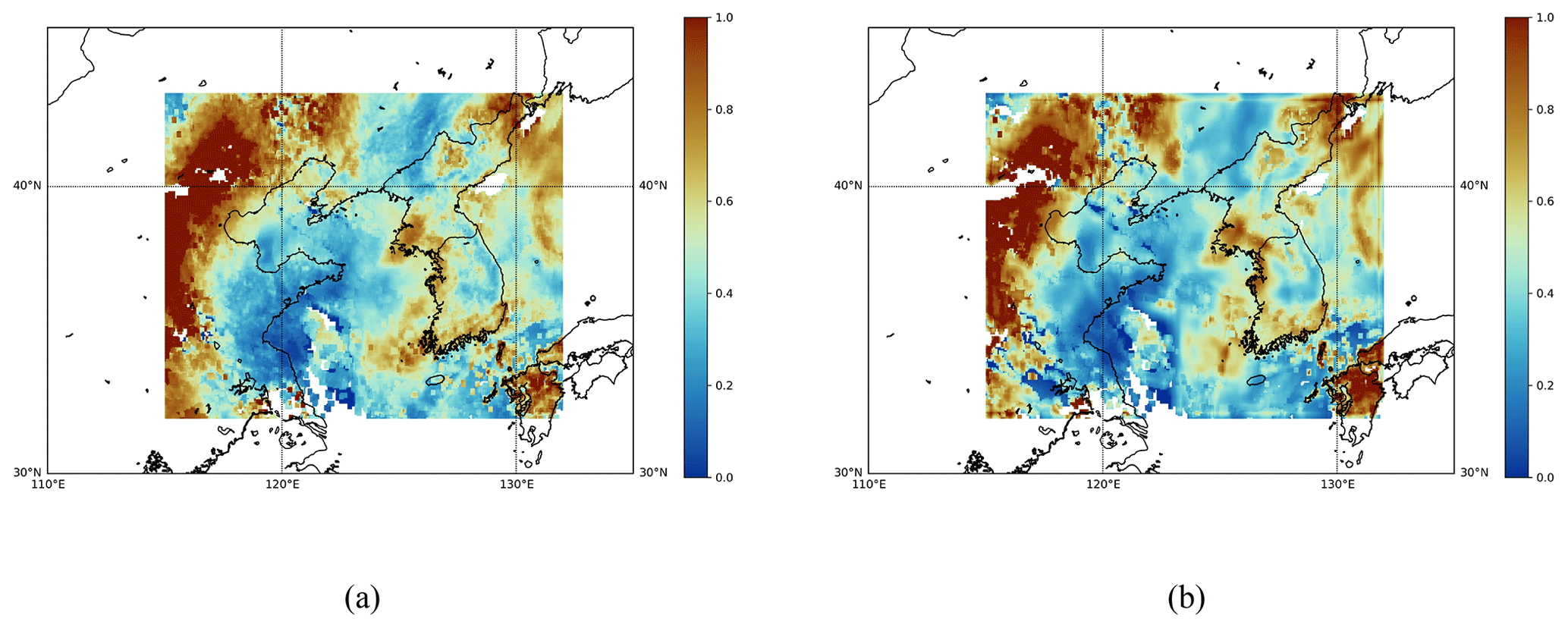
Figure C1 Daily mean field estimates of the GEMS L3 AOD product obtained on 1 April 2023 at a wavelength of 354 nm. (a) Simply averaged output. (b) Spatiotemporally merged output. The missing ratio for panel (a) is 0.0263, and the missing ratio for panel (b) is 0.0386.

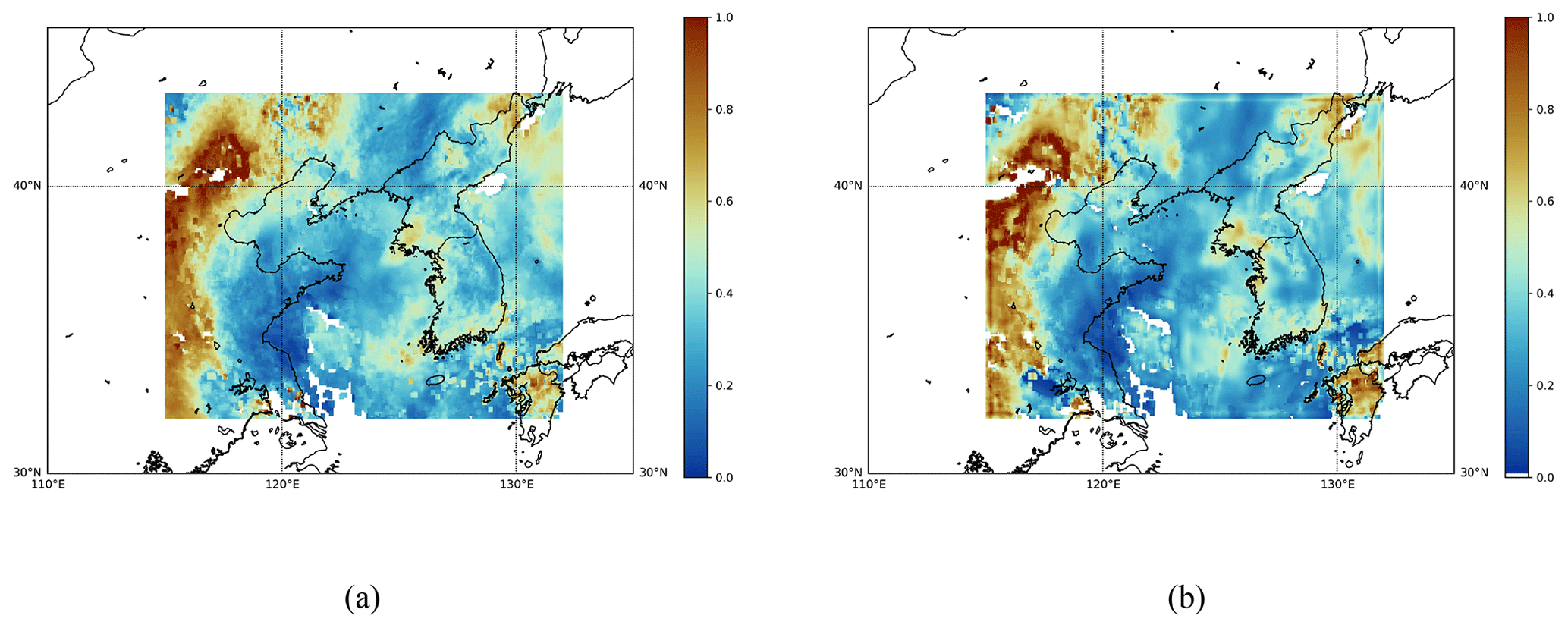
Figure C2 Daily mean field estimates of the GEMS L3 AOD product obtained on 1 April 2023 at a wavelength of 443 nm. (a) Simply averaged output. (b) Spatiotemporally merged output. The missing ratio for panel (a) is 0.0255, and the missing ratio for panel (b) is 0.0406.

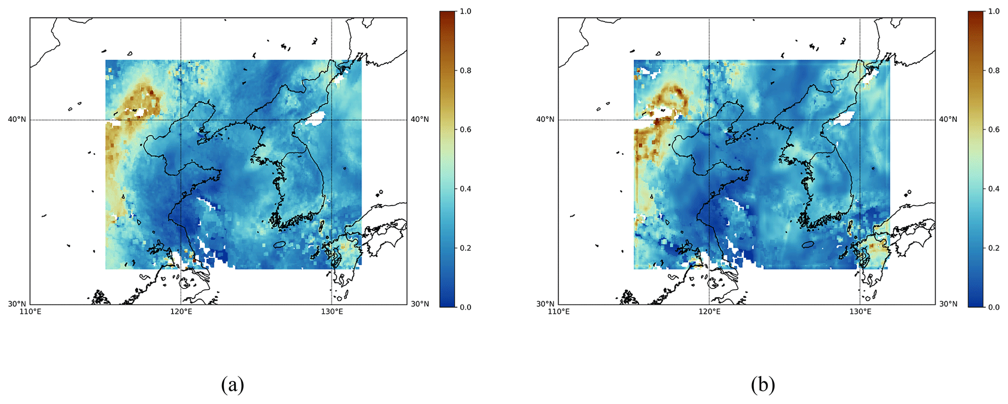
Figure C3 Daily mean field estimates of the GEMS L3 AOD product obtained on 1 April 2023 at a wavelength of 550 nm. (a) Simply averaged output. (b) Spatiotemporally merged output. The missing ratio for panel (a) is 0.0194, and the missing ratio for panel (b) is 0.0309.

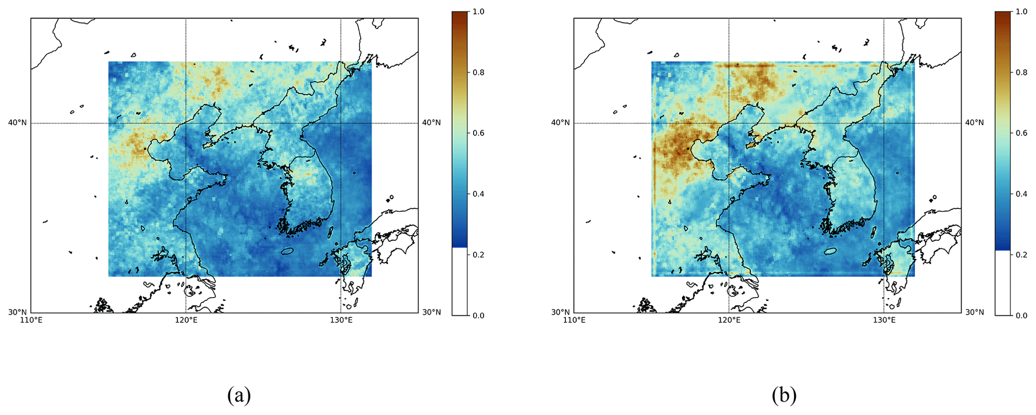
Figure C4 Monthly mean field estimates of the GEMS L3 AOD product obtained in April 2023 at a wavelength of 354 nm. (a) Simply averaged output. (b) Spatiotemporally merged output. The missing ratio for panel (a) is 0.0, and the missing ratio for panel (b) is 0.0.

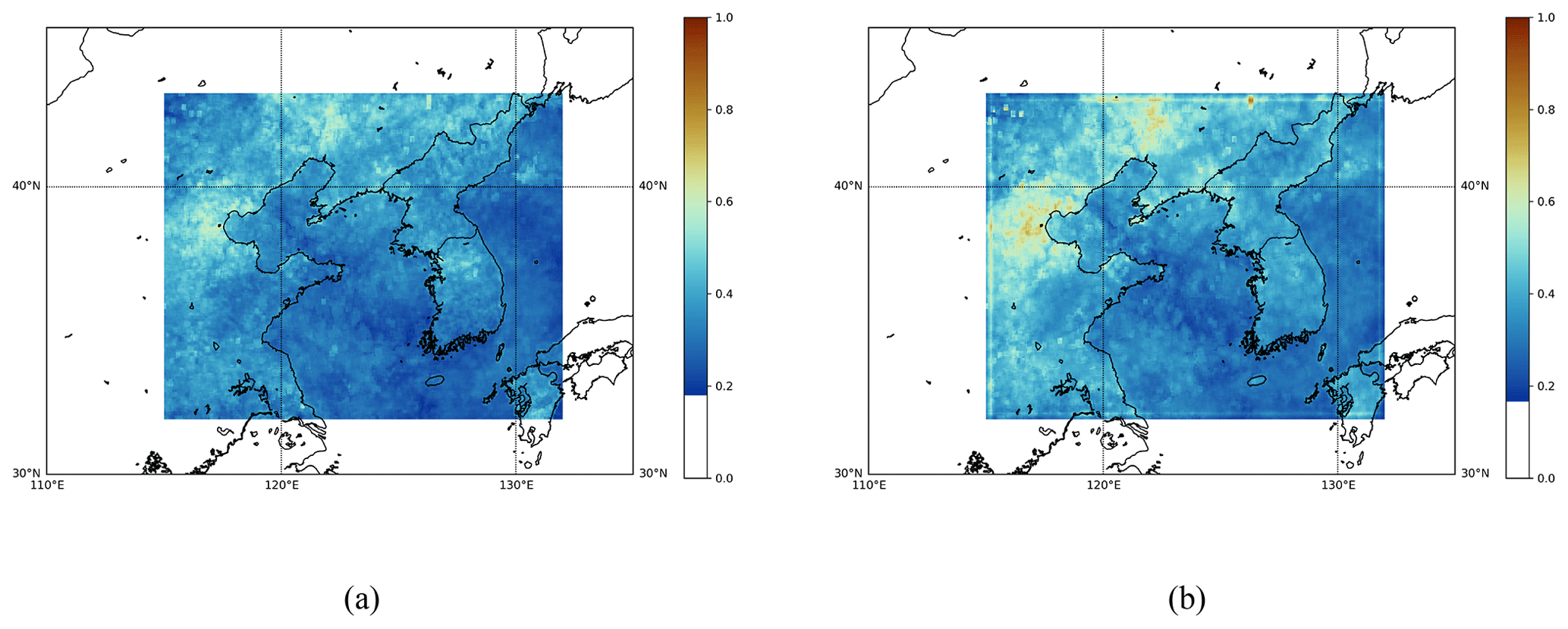
Figure C5 Monthly mean field estimates of the GEMS L3 AOD product obtained in April 2023 at a wavelength of 443 nm. (a) Simply averaged output. (b) Spatiotemporally merged output. The missing ratio for panel (a) is 0.0, and the missing ratio for panel (b) is 0.0.

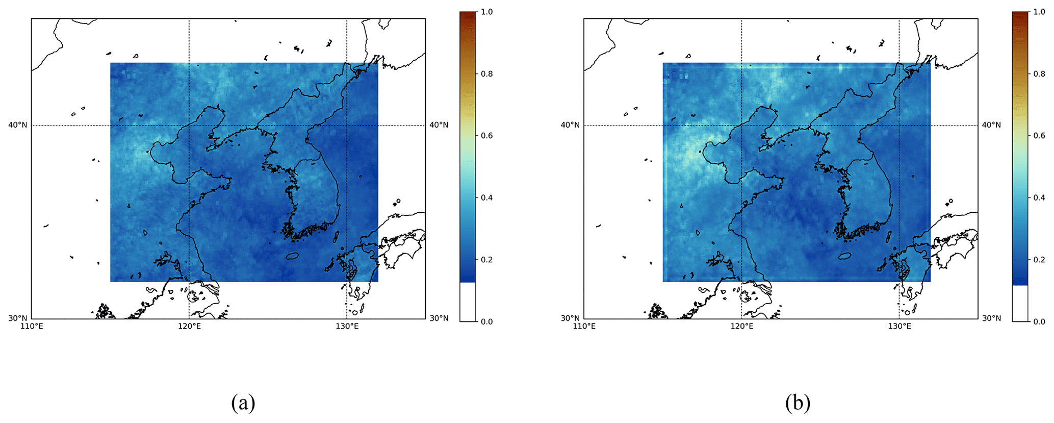
Figure C6 Monthly mean field estimates of the GEMS L3 AOD product obtained in April 2023 at a wavelength of 550 nm. (a) Simply averaged output. (b) Spatiotemporally merged output. The missing ratio for panel (a) is 0.0, and the missing ratio for panel (b) is 0.0.