Mapping the CO₂ total column retrieval performance from shortwave infrared measurements: synthetic impacts of the spectral resolution, signal-to-noise ratio, and spectral band selection

Satellites have been providing spaceborne observations of the total column of CO₂ (denoted $X_{{\mathrm{CO}}_{\mathrm{2}}}$) for over two decades now, and, with the need for independent verification of Paris Agreement objectives, many new satellite concepts are currently planned or being studied to complement or extend the instruments that already exist. Depending on whether they are targeting natural and/or anthropogenic fluxes of CO₂, the designs of these future concepts vary greatly. The characteristics of their shortwave infrared (SWIR) observations notably explore several orders of magnitude in spectral resolution (from $\mathit{\lambda }/\mathrm{\Delta }\mathit{\lambda }$ ∼ 400 for Carbon Mapper to $\mathit{\lambda }/\mathrm{\Delta }\mathit{\lambda }$ ∼ 25 000 for MicroCarb) and include different selections of spectral bands (from one to four bands, among which there are the CO₂-sensitive 1.6 µm and/or 2.05 µm bands). The very nature of the spaceborne measurements is also explored: for instance, the NanoCarb imaging concept proposes to measure CO₂-sensitive truncated interferograms, instead of infrared spectra like other concepts, in order to significantly reduce the instrument size. This study synthetically explores the impact of three different design parameters on the $X_{{\mathrm{CO}}_{\mathrm{2}}}$ retrieval performance obtained through optimal estimation: (1) the spectral resolution, (2) the signal-to-noise ratio (SNR) and (3) the spectral band selection. Similar performance assessments are completed for the exactly defined OCO-2, MicroCarb, Copernicus CO₂ Monitoring (CO₂M) and NanoCarb concepts. We show that improving the SNR is more efficient than improving the spectral resolution to increase $X_{{\mathrm{CO}}_{\mathrm{2}}}$ precision when perturbing these parameters across 2 orders of magnitude, and we find that a low SNR and/or a low spectral resolution yield $X_{{\mathrm{CO}}_{\mathrm{2}}}$ with vertical sensitivities that give more weight to atmospheric layers close to the surface. The exploration of various spectral band combinations illustrates, especially for lower spectral resolutions, how including an O₂-sensitive band helps to increase the optical path length information and how the 2.05 µm CO₂-sensitive band contains more geophysical information than the 1.6 µm band. With very different characteristics, MicroCarb shows a CO₂ information content that is only slightly higher than that of CO₂M, which translates into $X_{{\mathrm{CO}}_{\mathrm{2}}}$ random errors that are lower by a factor ranging from 1.1 to 1.9, depending on the observational situation. The performance of NanoCarb for a single pixel of its imager is comparable to those of concepts that measure spectra at low SNR and low spectral resolution, but, as this novel concept would observe a given target several times during a single overpass, its performance improves when combining all the observations. Overall, the broad range of results obtained through this synthetic $X_{{\mathrm{CO}}_{\mathrm{2}}}$ performance mapping hint at the future intercomparison challenges that the wide variety of upcoming CO₂-observing concepts will pose.

1 Introduction

Anthropogenic emissions of carbon dioxide (CO₂) are the main driver of climate change (IPCC, 2021). The current understanding of the global carbon cycle is based on comparisons of results from bottom-up methods, which explicitly model CO₂-emitting and CO₂-absorbing mechanisms, with those from top-down approaches, which rely on a set of CO₂ atmospheric concentration observations to find the CO₂ fluxes that best fit those observations (Friedlingstein et al., 2022). This last approach, called inverse atmospheric transport (Ciais et al., 2010), can ingest in situ observations and/or spaceborne remote estimations of the CO₂ atmospheric concentration. The latter are produced through inverse radiative transfer, which finds the atmospheric states (including the CO₂ concentration) that best fit infrared satellite measurements made from space.

Shortwave infrared (SWIR) satellite measurements, which are sensitive to – among others – CO₂ concentration close to the surface, where fluxes take place, have been exploited for two decades to retrieve the column-averaged dry-air mole fraction of CO₂ (also called the “total column” and denoted $X_{{\mathrm{CO}}_{\mathrm{2}}}$). The pioneering ESA Scanning Imaging Absorption Spectrometer for Atmospheric Chartography (SCIAMACHY) instrument (Bovensmann et al., 1999) was the first to provide a global $X_{{\mathrm{CO}}_{\mathrm{2}}}$ dataset. Its mission ended in 2012, and it was followed by the – still flying – JAXA/NIES Greenhouse gases Observing SATellites (GOSAT and GOSAT-2; Inoue et al., 2016; Noël et al., 2021; Taylor et al., 2022), the NASA Orbiting Carbon Observatory-2 (OCO-2) and OCO-3 (Taylor et al., 2023), and the Chinese TanSat (Yang et al., 2020). The global $X_{{\mathrm{CO}}_{\mathrm{2}}}$ datasets produced by these missions have found applications for the study of natural carbon fluxes at a global scale (e.g. Chevallier et al., 2019; Peiro et al., 2022) and also (even though it was not their primary objective) for the monitoring of point-source anthropogenic emissions (Nassar et al., 2021; Reuter et al., 2019; Zheng et al., 2020).

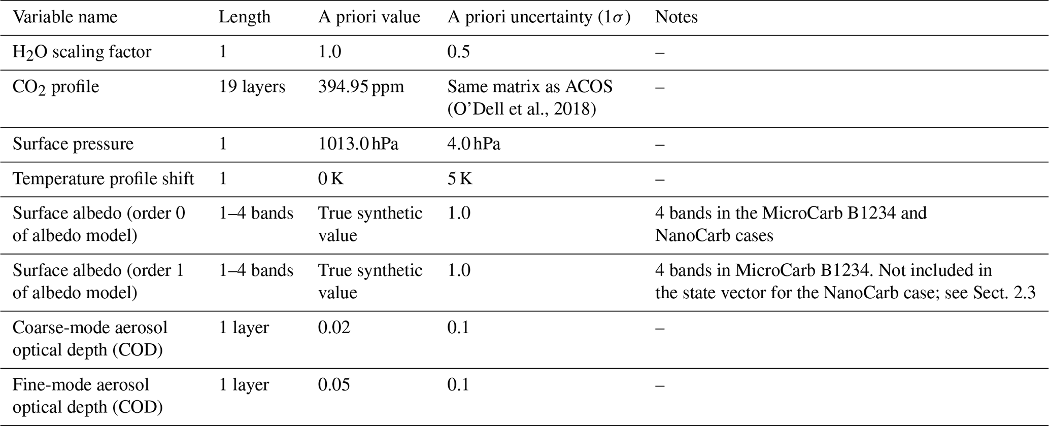
Table 1 Measurement characteristics for some of the upcoming or studied SWIR CO₂-observing satellite concepts.

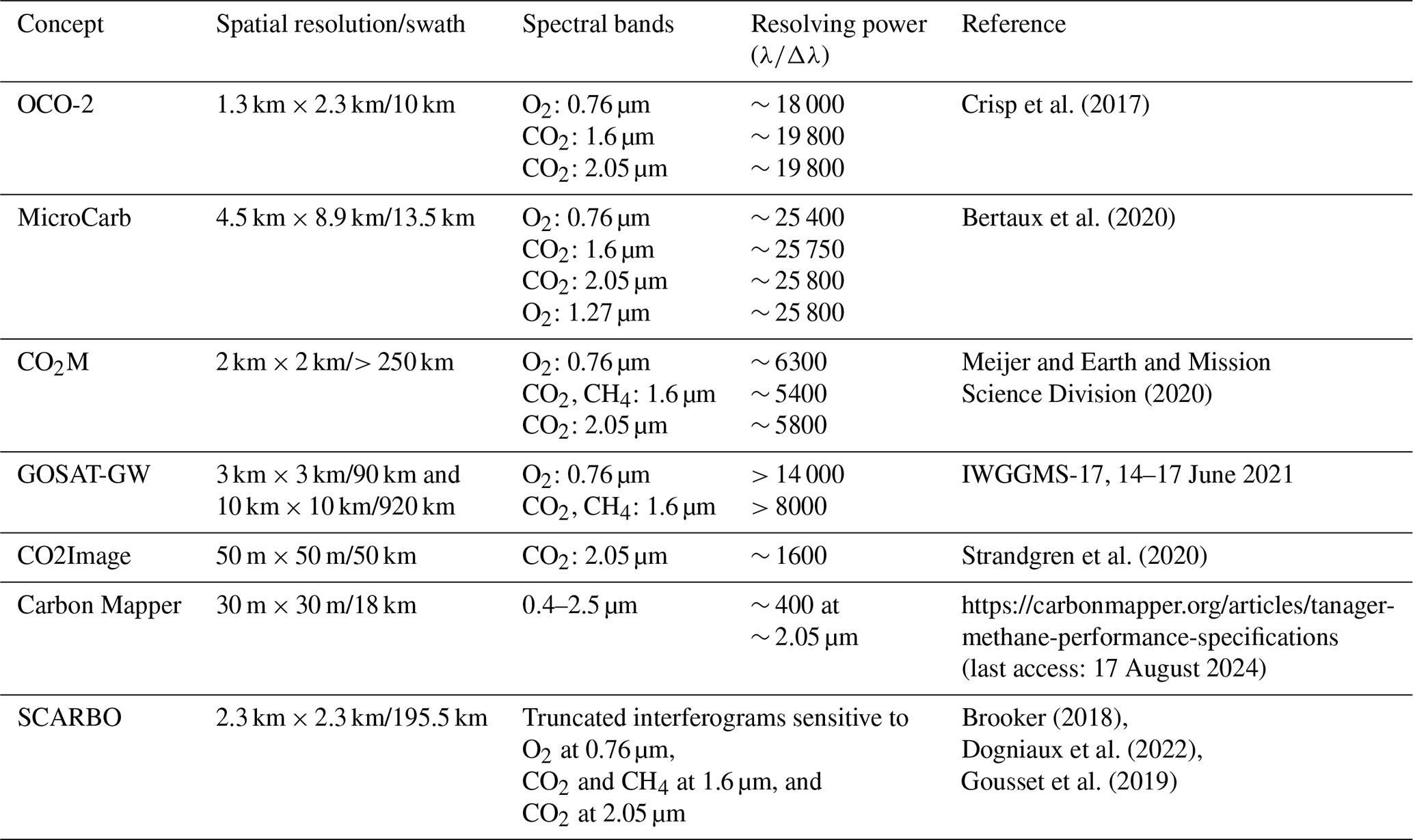
These different missions will be followed by various concepts that are already planned or still being studied. First, the planned Centre national d'études spatiales (CNES) MicroCarb mission (Bertaux et al., 2020; Pascal et al., 2017) is quite similar to OCO-2 regarding its observation strategy (in terms of its spatial and spectral resolution, as shown in Table 1, although it includes an extra O₂-sensitive band) and mainly aims to provide information on natural CO₂ fluxes. The 2015 Paris Agreement and the 5-year global stocktake system it set up have put in motion a global ambition for spaceborne monitoring of anthropogenic greenhouse gas emissions (mainly CO₂ and methane, but the latter is not the focus of this work). Indeed, urban areas, which account for 0.5 % of the ice-free continental surface (Liu et al., 2020; Lwasa et al., 2022), are responsible for 70 % of all fossil-fuel-related emissions (Duren and Miller, 2012). In favourable meteorological conditions, CO₂ plumes arise from either hotspots, such as megacities, or point sources, such as coal-fired power plants (Kuhlmann et al., 2019). Those plumes may then be observed with spaceborne SWIR imagers, depending on their precision and spatial resolution, and the emission rate associated with the imaged plume can then be inferred either with plume analysis and/or mass-balance approaches (Bovensmann et al., 2010; Varon et al., 2018) or within more usual atmospheric inversion schemes (Broquet et al., 2018; Pillai et al., 2016). Because an infrared detector has a limited number of pixels, future – planned or studied – CO₂-imaging concepts explore various trade-offs between the spatial and spectral resolution and spectral band selection, and they even compromise in terms of the very nature of the measurements made by the instrument when other constraints such as size (and thus costs) are taken into consideration. These concepts include – among others – the European Copernicus CO₂ Monitoring (CO₂M; Meijer and Earth and Mission Science Division, 2020) mission, the Japanese Global Observing SATellite for Greenhouse gases and Water cycle (GOSAT-GW; Matsunaga and Tanimoto, 2022), the American non-profit Carbon Mapper initiative (https://carbonmapper.org/, last access: 17 August 2024) based on the Next-Generation NASA Airborne Visible/Infrared Imaging Spectrometer (Cusworth et al., 2021; Hamlin et al., 2011), the German CO2Image concept (Strandgren et al., 2020; Wilzewski et al., 2020) and the European Space CARBon Observatory (SCARBO) H2020 concept, which does not measure spectra, only truncated interferograms (Brooker, 2018; Dogniaux et al., 2022; Gousset et al., 2019). Table 1 gathers the characteristics of upcoming or studied SWIR CO₂-observing satellite concepts, which are provided either in scientific articles (in which case citations are provided), in conference presentations (in which case just the conference name and dates are given) or on websites (in which case just the hyperlink is given), as some of these concepts are quite recent.

The characteristics of an observing concept (nature of measurement, spectral resolution, spectral band selection and signal-to-noise ratio) translate into an $X_{{\mathrm{CO}}_{\mathrm{2}}}$ retrieval performance that comprises (1) the random error, (2) the systematic error and (3) the vertical sensitivity. First, the $X_{{\mathrm{CO}}_{\mathrm{2}}}$ random error (or precision) impacts the a posteriori uncertainties of fluxes estimated in usual inverse atmospheric schemes (Rayner and O'Brien, 2001) and the detectability of CO₂ plumes for imaging concepts (Kuhlmann et al., 2019). In addition to random errors, systematic errors can hamper $X_{{\mathrm{CO}}_{\mathrm{2}}}$ retrievals. Those can, for example, be due to forward radiative transfer modelling errors, like aerosol misknowledge (Houweling et al., 2005; Reuter et al., 2010), or the a priori misknowledge of atmospheric state parameters (Connor et al., 2008). Spatially correlated systematic errors are especially detrimental in inverse atmospheric schemes (Broquet et al., 2018; Chevallier et al., 2007), whereas scene-wide systematic errors that do not correlate with the plume shape can cancel out when applying plume analysis techniques. Finally, the retrieved CO₂ total columns must be characterized by their vertical sensitivity, which illustrates the atmospheric levels to which retrievals are sensitive (Boesch et al., 2011; Buchwitz et al., 2005).

The impacts of SWIR measurement characteristics on $X_{{\mathrm{CO}}_{\mathrm{2}}}$ retrieval performance have been partially examined in previous studies that relied on real measurements. For instance, Galli et al. (2014) assessed the performance of $X_{{\mathrm{CO}}_{\mathrm{2}}}$ retrievals from GOSAT measurements for which spectral resolution was degraded by up to 6 times ($\mathit{\lambda }/\mathrm{\Delta }\mathit{\lambda }\sim \mathrm{3000}--\mathrm{20}\mathrm{000})$, and Wu et al. (2020) performed a similar exercise with OCO-2 measurements degraded at CO₂M spectral resolution. Spectral band selection has also been studied: Wu et al. (2019) performed retrievals only using the 2.05 µm band of OCO-2 measurements, and Wilzewski et al., (2020) considered single-band observations from spectrally degraded 1.6 µm/2.05 µm GOSAT band measurements ($\mathit{\lambda }/\mathrm{\Delta }\mathit{\lambda }$ ∼ 700–8100/6150, respectively).

In this work, we perform a systematic survey that synthetically explores the impact of the spectral resolution, signal-to-noise ratio (SNR) and spectral band selection – three design parameters for SWIR CO₂-observing satellite concepts – on $X_{{\mathrm{CO}}_{\mathrm{2}}}$ retrieval performance (SNR-related precision, degrees of freedom, vertical sensitivity and smoothing error, with the accuracy excluded). These choices are motivated by the characteristics gathered in Table 1. Indeed, 2 orders of magnitude in resolving power ($\mathit{\lambda }/\mathrm{\Delta }\mathit{\lambda }$) separate Carbon Mapper (AVIRIS-NG) from MicroCarb. Exploring a wide range of SNR values on top of different resolving powers will help to encompass all possible performance results from a wide variety of concepts that measure SWIR spectra. Finally, because CO2Image is planned to measure only the 2.05 µm band and GOSAT-GW will only measure the 0.76 and 1.6 µm bands, we will also study the impact of choosing different combinations of spectral bands. Synthetic calculations performed for a fictitious concept with varying design parameters will help to map a large space of possible $X_{{\mathrm{CO}}_{\mathrm{2}}}$ retrieval performances to which those of the peculiar SCARBO concept will be compared, along with those of the current OCO-2 and upcoming MicroCarb and CO₂M missions.

This article is structured as follows. Section 2 describes the observing concepts considered in this work, and Sect. 3 details the materials and methods. Section 4 describes the results obtained for a fictitious concept with varying design parameters and discusses them. It first focuses on the impact of spectral resolution and SNR, then on the impact of spectral resolution and spectral band selection, for which it also explores geophysical information entanglements. Finally, Sect. 5 discusses the performance results obtained for the exactly defined OCO-2, MicroCarb and CO₂M concepts, along with those of the peculiar NanoCarb concept, and how they compare to those of the fictitious concept with varying design parameters. Section 6 highlights the conclusions of this work.

2 SWIR CO₂-observing satellite concepts

In this section, we provide the measurement characteristics that are used to model the different upcoming – real or fictitious – SWIR CO₂-observing satellite concepts. In order to reduce the number of dimensions to explore, we consider, for the purpose of this study, that the spectra-measuring concepts have identical resolving powers $\mathit{\lambda }/\mathrm{\Delta }\mathit{\lambda }$ across all their spectral bands as well as a constant spectral sampling ratio of 3 (which is the case for both MicroCarb and CO₂M and is a design hypothesis for CO2Image). All instrument spectral response functions (ISRFs) are treated as Gaussian functions with a full width at half maximum (FWHM, Δλ) calculated from the resolving power $\mathit{\lambda }/\mathrm{\Delta }\mathit{\lambda }$, where λ is the average spectral band wavelength.

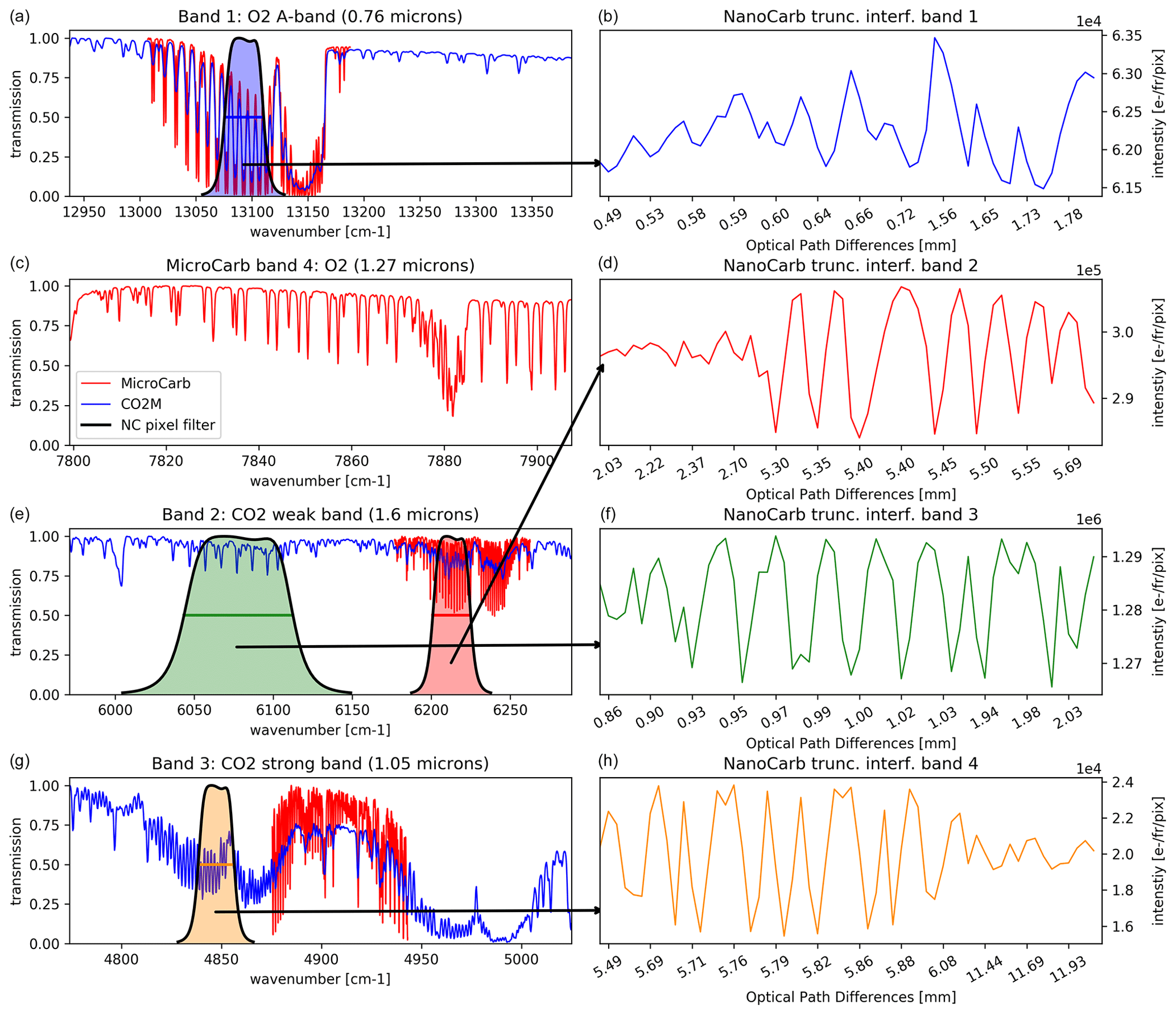
Figure 1 Examples of CO₂M (blue) and MicroCarb (red) transmissions (a, c, e, g) and NanoCarb truncated interferograms (in photo-electron per frame per pixel; b, d, f, h) for a vegetation-like albedo with a solar zenith angle of 50°. Arrows link NanoCarb bands to their respective narrowband filters (the horizontal coloured lines denote their FWHMs), which are shown on top of the CO₂M and MicroCarb transmissions.

2.1 OCO-2, MicroCarb and CO₂M

We consider three explicitly described upcoming concepts that measure and will measure SWIR spectra: OCO-2, MicroCarb and the Copernicus CO₂ Monitoring (CO₂M) concept. Figure 1a, c, e and g illustrate MicroCarb and CO₂M observations.

The Orbiting Carbon Observatory-2 (OCO-2) has been providing $X_{{\mathrm{CO}}_{\mathrm{2}}}$ observations from SWIR measurements for close to a decade (Taylor et al., 2023). We include this instrument in order to assess how the synthetic results obtained here relate to results obtained from real data. Our modelling of OCO-2 observations relies on instrument functions and noise models provided in OCO-2 L1b Science and Standard L2 products of the Atmospheric Carbon Observation from Space algorithm, version 8 (ACOS; O'Dell et al., 2018). These files are not from the latest version (v10) of the OCO-2 data, but the major reprocessing of v8 to v10 did not include significant changes in instrument parameters (Taylor et al., 2023), so we assess that our input data are acceptable for this synthetic study.

Table 2 MicroCarb measurement characteristics used in this work.

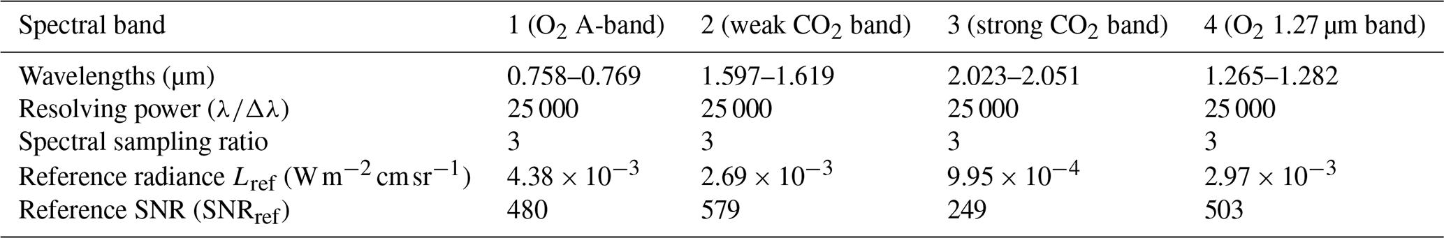
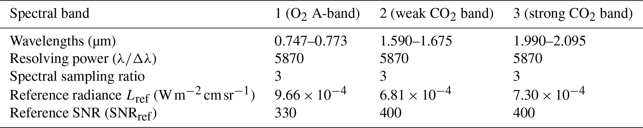
Table 3 CO₂M spectrometer measurement characteristics used in this work.

MicroCarb (Bertaux et al., 2020; Pascal et al., 2017) is the upcoming CNES CO₂-observing mission that will acquire SWIR spectra at high spectral resolution, thus following in the steps of the currently flying OCO-2. Besides the increase in spectral resolution, its main novelty is the addition of the O₂ 1.27 µm band that will provide additional optical path length information at wavelengths closer to those that have CO₂ sensitivity, which may help to reduce aerosol-related errors. MicroCarb aims at retrieving $X_{{\mathrm{CO}}_{\mathrm{2}}}$ with a precision below 1 ppm and with the lowest possible systematic errors. In this work, we use the measurement characteristics presented in Table 2 to model the MicroCarb concept. In Sect. 5, where MicroCarb results are presented, the impact on performance of using both or just one of the O₂-sensitive bands will be discussed.

The Copernicus CO₂ Monitoring (CO₂M) mission (Meijer and Earth and Mission Science Division, 2020) is the upcoming space component of the operational European anthropogenic CO₂ emissions Monitoring and Verification Support capacity (CO₂MVS; Janssens-Maenhout et al., 2020). Its design is a compromise between the spatial and spectral resolutions, the swath and the spectral band width, and it aims to provide imaging of $X_{{\mathrm{CO}}_{\mathrm{2}}}$ with a random error lower than 0.7 ppm and systematic errors that are as low as possible (Meijer and Earth and Mission Science Division, 2020). In this work, we use the spectrometer measurement characteristics presented in Table 3 to model the CO₂M concept. Besides the spectrometer, the CO₂M mission will also include a multi-angle polarimeter, which is an instrument dedicated to the observation of aerosols. Its results are expected to help to better constrain their interfering effect on $X_{{\mathrm{CO}}_{\mathrm{2}}}$ retrievals and to improve their precision and accuracy (Rusli et al., 2021). Here, we only study the CO₂M spectrometer alone, so the results that we obtain do not reflect the comprehensive theoretical CO₂M mission performance.

2.2 The fictitiously varying CO₂M concept (CVAR)

In order to grasp the full extent of the upcoming or studied SWIR CO₂-observing satellite concepts, we also consider a fictitious concept that has the same characteristics as CO₂M apart from its resolving power $\mathit{\lambda }/\mathrm{\Delta }\mathit{\lambda }$, SNR and spectral band selection. This varying concept will be hereafter referred to as “CVAR”.

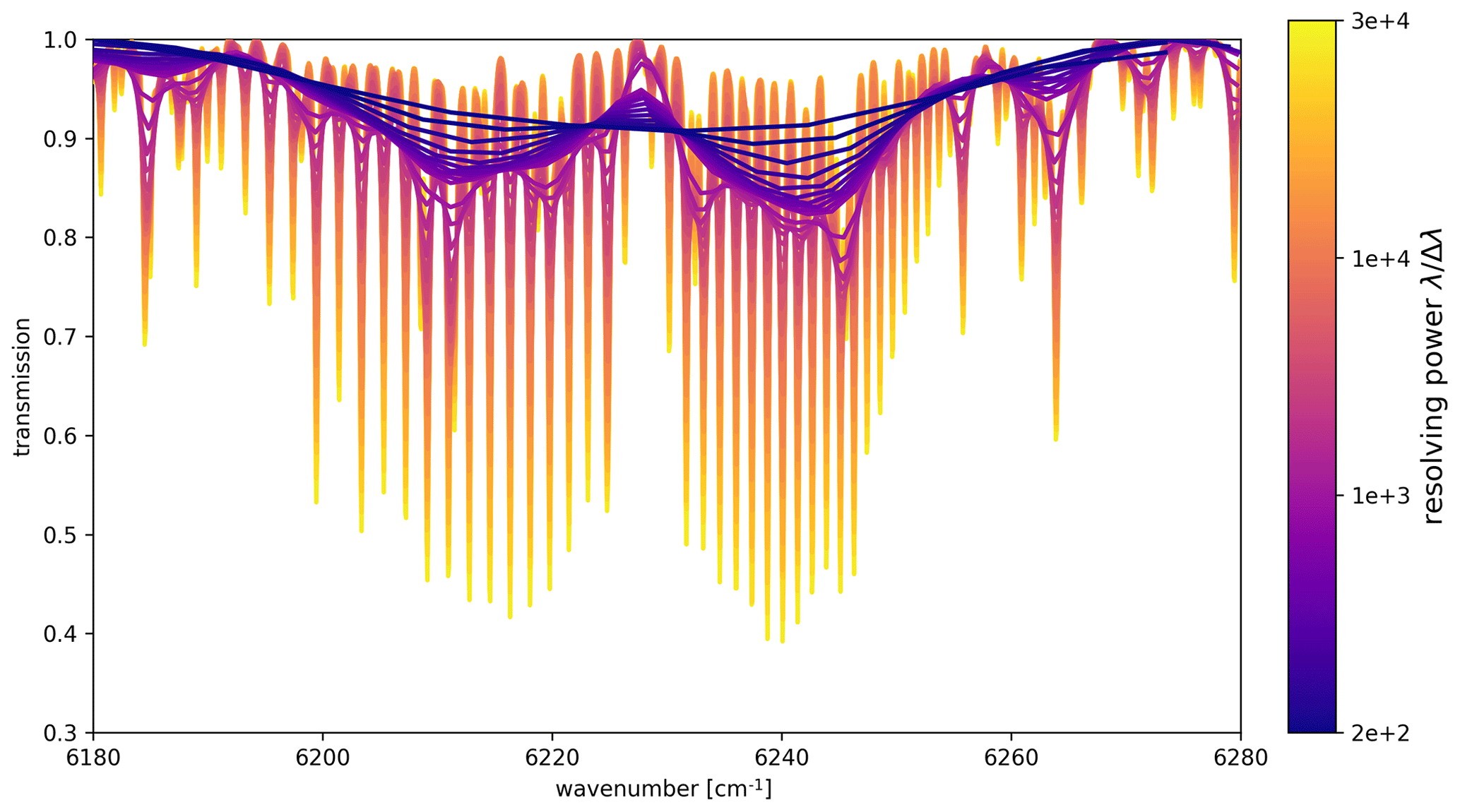
Figure 2 CO₂-sensitive 1.6 µm band observed with a resolving power $\mathit{\lambda }/\mathrm{\Delta }\mathit{\lambda }$ ranging from 200 to 30 000.

First, we consider resolving-power values ranging from 200 to 30 000 (the list of exact resolving-power values that are considered is given in Table S1 in the Supplement). Figure 2 illustrates the impact of spectral resolution on the CO₂ absorption band around 1.6 µm. For the lowest resolving power $\mathit{\lambda }/\mathrm{\Delta }\mathit{\lambda }=\mathrm{200}$, the “two-lobed” P-R branch structure of this CO₂ absorption band (Liou, 2002) is not visible. It fully appears from $\mathit{\lambda }/\mathrm{\Delta }\mathit{\lambda }$ = 1000 upwards. Individual absorption lines become visible but are not fully resolved for $\mathit{\lambda }/\mathrm{\Delta }\mathit{\lambda }$ values between about 1000 and 10 000. Only when $\mathit{\lambda }/\mathrm{\Delta }\mathit{\lambda }$ > 10 000 do the whole P-R band structure and individual absorption lines fully appear. Given that the fixed CO₂M spectral band intervals are quite large compared to those of MicroCarb, the choice of using the CO₂M band intervals for exploring the impact of the resolving power on $X_{{\mathrm{CO}}_{\mathrm{2}}}$ retrieval performance is a reasonable compromise between high-resolution instruments that measure narrow spectral bands (e.g. MicroCarb or OCO-2) and low-resolution instruments that measure continuous spectra (e.g. Carbon Mapper, which measures from 0.4 to 2.5 µm). Thus, this compromise yields fictitiously large spectral bands for CVAR cases with high resolving-power values and corresponds to a window selection approach for observations with low spectral resolution, similar to what is actually done to process AVIRIS-NG measurements (Cusworth et al., 2021).

In addition to the spectral resolution, we also consider the impact of the SNR in this study. This will help us to explore the performance of a wider range of SWIR CO₂-observing satellite concepts. We will cover 2 orders of magnitude in the noise level by applying a spectral-band-specific factor ranging from 0.1 to 10 to the CO₂M SNR values given in Table 3. The impacts of both the spectral resolution and SNR on $X_{{\mathrm{CO}}_{\mathrm{2}}}$ retrieval performance results are presented and discussed in Sect. 4.1.

Finally, in addition to the spectral resolution but separately from the SNR, we consider the impact of spectral band selection. This will help us to encompass upcoming or studied single- or dual-band observing concepts such as CO2Image or GOSAT-GW, respectively. All CO₂M spectral band combinations containing at least one CO₂-sensitive band will be explored: B2, B12, B3, B13, B23 and B123 (B denotes “band” and is followed by the CO₂M spectral band numbers considered in the combination). The impacts of both the spectral resolution and spectral band selection on $X_{{\mathrm{CO}}_{\mathrm{2}}}$ retrieval performance results and geophysical information entanglement are presented and discussed in Sect. 4.2.

2.3 The SCARBO concept and NanoCarb

The Space CARBon Observatory (SCARBO) concept (Brooker, 2018) is quite different from all the other concepts mentioned in this article. It relies on a miniaturized static Fabry–Perot interferometer, named NanoCarb, that measures truncated interferograms at optical path differences (OPDs) which are optimally sensitive to CO₂ and to some other interfering geophysical variables (Gousset et al., 2019). Because of their very nature, these truncated interferograms are sensitive to the periodic signature of CO₂ in the infrared spectrum. As in Dogniaux et al. (2022), here we use the latest design of the NanoCarb instrument, currently considered with an ∼ 200 km swath and a 2.3 km × 2.3 km spatial resolution. The optimal OPD selection accounts for CO₂ information entanglements with H₂O and aerosols, neglects the atmospheric temperature, and assumes that albedo is constant across each band (Gousset et al., 2019). It measures truncated interferograms that are sensitive to four spectral bands, as shown in the right panels of Fig. 1, which are associated with the narrowband filters shown in Fig. 1a, c, e and g (follow the arrows). Their FWHMs are 35, 24, 69 and 18 cm⁻¹ for bands 1 to 4, respectively. NanoCarb has a two-dimensional field of view (FOV; 170 across-track × 102 along-track pixels in the current design) that observes a fixed location on the ground from different viewing angles as it flies over it. The up to 102 $X_{{\mathrm{CO}}_{\mathrm{2}}}$ retrievals that can be done for the same location on the ground are then combined to yield only one unique retrieval result with a reduced random error (assuming independent observations). Dogniaux et al. (2022) details the NanoCarb concept performance results and its current shortcomings. One of the main results is that NanoCarb performance decreases close to the FOV edges, so we will only focus here on the central FOV pixel and central along-track row of pixels. It also explains that the CO₂ and interfering geophysical variable information contents are entangled in NanoCarb truncated interferograms. This specific shortcoming will be further detailed in this article.

3 Materials and methods

3.1 Atmospheric and observational situations

As this study focuses on the impact of instrument design parameters on $X_{{\mathrm{CO}}_{\mathrm{2}}}$ retrieval performance, we purposefully limit the number of atmospheric conditions that we include. We consider 12 atmospheric and observational situations that explore three surface albedo models (soil, vegetation and desert, denoted SOL, VEG and DES, respectively; their average values over the SWIR spectral bands are given in Table S2) generated from the ASTER spectral library (Baldridge et al., 2009) and four solar zenith angles (hereafter SZA, 0, 25, 50 and 70°). A given situation will be referred to by the short name of its albedo model followed by the SZA; e.g. VEG-50° corresponds to the situation where the albedo is representative of vegetation and the SZA is equal to 50°.

For these 12 situations, the measurements are made at nadir (a viewing zenith angle equal to 0°). We use a typically European atmospheric situation (vertical temperature and water vapour profiles), taken as the average of the mid-latitude temperate atmospheric profiles included in the Thermodynamic Initial Guess Retrieval (TIGR) climatology library (Chedin et al., 1985; Chevallier et al., 1998). For this synthetic performance study, we consider a constant vertical CO₂ concentration profile of 394.95 ppm. The surface pressure is constant and set at 1013 hPa. To mimic possible pollution over the European continent, we include fine-mode aerosols (representative of soot) between 0 and 2 km of altitude and coarse-mode aerosols (representative of minerals) between 2 and 4 km of altitude (this choice is supported by desert dust layers that are transported over Europe, as described by Papayannis et al., 2008).

3.2 Performance evaluation with optimal estimation

3.2.1 General aspects

Optimal estimation (Rodgers, 2000) offers an ideal framework for the evaluation of $X_{{\mathrm{CO}}_{\mathrm{2}}}$ retrieval performance. It has been extensively described in other publications (e.g. Connor et al., 2008), so only its essential aspects are described in this article. Given a state vector x that contains parameters that describe the atmospheric and surface states and a measurement vector y that contains the infrared observation made from space by a studied concept, OE enables us to provide the geophysical state that best fits the measurement made from space, thus giving a satisfying solution to the following equation:

$$\begin{array}{}\text{(1)}& \mathit{y}=F\left(\mathit{x}\right)+\mathit{ϵ},\end{array}$$

where F is the forward radiative transfer model that allows us to simulate spaceborne infrared observations from geophysical state parameters and ϵ is the spaceborne measurement uncertainty. Because this inverse problem is ill posed, OE brings in a priori information that helps to better constrain the estimation. This a priori information can be seen as the knowledge of the geophysical state one would have before using the information contained in the spaceborne measurement (e.g. taken from climatologies). It is given in the form of an a priori state vector x_a, which is characterized by its uncertainty, as given in the a priori state covariance matrix S_a.

The retrieved geophysical state that best fits the measurement made from space and the a priori information is called the maximum-likelihood a posteriori state and is denoted $\widehat{\mathit{x}}$. Its a posteriori covariance matrix, which describes the uncertainty of the retrieved state, is denoted $\widehat{\mathbf{S}}$ and computed using the following equation:

$$\begin{array}{}\text{(2)}& \widehat{\mathbf{S}}={\left[{\mathbf{S}}_{\mathrm{a}}^{-\mathrm{1}}+{\mathbf{K}}^{\mathrm{T}}{\mathbf{S}}_{\mathrm{e}}^{-\mathrm{1}}\mathbf{K}\right]}^{-\mathrm{1}},\end{array}$$

where S_e is the a priori covariance matrix of the measurement vector describing measurement/forward modelling uncertainties and K is the Jacobian matrix containing the partial derivatives of the measurement with respect to the state vector parameters. Its elements for a usual SWIR spectrum and a corresponding NanoCarb truncated interferogram are illustrated in the Supplement (see Figs. S1 and S2).

Another useful OE result is the averaging kernel matrix, denoted A, which describes how the retrieved state $\widehat{\mathit{x}}$ relates to the true – but unknown – geophysical state:

$$\begin{array}{}\text{(3)}& \mathbf{A}={\displaystyle \frac{\partial \widehat{\mathit{x}}}{\partial \mathit{x}}}=\widehat{\mathbf{S}}{\mathbf{K}}^{\mathrm{T}}{\mathbf{S}}_{\mathrm{e}}^{-\mathrm{1}}\mathbf{K}.\end{array}$$

The diagonal elements of A are the state vector elements' degrees of freedom, which provide a measure of the geophysical information obtained from the measurement through the OE process. Degrees of freedom close to 1 highlight a high contribution of the measurement to the estimation of a given state vector parameter, whereas degrees of freedom close to 0 denote a low contribution of the measurement and a high contribution of the a priori information. Finally, A also enables the computation of the $X_{{\mathrm{CO}}_{\mathrm{2}}}$ averaging kernel, which describes its vertical sensitivity (Connor et al., 2008). It shows the atmospheric layers that the retrieval is the most sensitive to and is essential for characterizing and correctly exploiting the retrieved $X_{{\mathrm{CO}}_{\mathrm{2}}}$.

Table 4 State vector used for the performance evaluation.

3.2.2 Forward and inverse setups for performance evaluation

We use the 5AI inverse model (Dogniaux et al., 2021), which relies on the 4A/OP radiative transfer model (Scott and Chédin, 1981), to build the Jacobian matrix K. These forward radiative transfer simulations rely on the GEISA 2015 spectroscopic database (Jacquinet-Husson et al., 2016) along with line-mixing effects for CO₂ (Lamouroux et al., 2015) and collision-induced absorption in the O₂ 0.76 µm band (Tran and Hartmann, 2008). Multiple scattering is taken into account through the coupling of 4A/OP with LIDORT (Spurr, 2002), and the aerosol optical properties are taken from the OPAC library, which uses lognormal size distributions (Hess et al., 1998). For the performance study performed here, we assume that these optical properties, including their spectral dependences, are perfectly known, thus allowing the transfer of information when combining different spectral bands. Finally, the atmospheric model is discretized into 20 atmospheric layers that bound 19 layers, as done by the ACOS algorithm (O'Dell et al., 2018). Airglow emission, which impacts the MicroCarb 1.27 µm band (Bertaux et al., 2020), is not included here in the 4A/OP simulations.

We include in the state vector all the main geophysical variables that are necessary to model SWIR spaceborne measurements. These are listed in Table 4, along with their a priori values and uncertainties. This selection of state vector parameters is used for all exactly defined concepts (with the small exception of the albedo slope for NanoCarb) and CVAR experiment cases because the goal of this study is to explore the impact of design parameters on performance. Using a similar estimation scheme across all resolving powers helps us achieve this goal. However, we do realize that, in practice, less geophysical elements would be fitted for low-resolving-power observations (e.g. Cusworth et al., 2021). Finally, the measurement noise model that fills the diagonal of S_e is calculated, as in Buchwitz et al. (2013), with a reference radiance L_ref and a reference signal-to-noise ratio SNR_ref:

$$\begin{array}{}\text{(4)}& {\mathit{\sigma }}_{\mathrm{e}}=\left\{\begin{array}{lcl}{L}_{\mathrm{ref}}/{\mathrm{SNR}}_{\mathrm{ref}},& \text{if}& L<L_{\mathrm{ref}}\\ L/\left({\text{SNR}}_{\mathrm{ref}}\sqrt{L/L_{\mathrm{ref}}}\right),& \text{if}& L\ge L_{\mathrm{ref}},\end{array}\right.\end{array}$$

where σ_e is the noise model for a given spectral sample and L is the radiance for a given spectral sample. Here, the matrix S_e only includes measurement noise, so the uncertainty (or precision) results obtained from the matrix $\widehat{\mathbf{S}}$ will only be related to measurement noise. In practice, smoothing errors from CO₂ and non-CO₂ state vector parameters add up to the uncertainty (Connor et al., 2008). Finally, the uncertainty evaluated for real data is typically larger than the uncertainty obtained from optimal estimation calculations, as model-related errors (the uncertainty in the albedo spectral dependence, spectroscopy errors, etc.) are also encompassed by such evaluations. For example, at low resolving powers, the complexity of the spectral dependence of surface reflectance can lead to significant errors (e.g. for methane; Ayasse et al., 2018) that will not be accounted for here, and, at high resolving power, real-data uncertainties are evaluated to be twice as large as the theoretical uncertainty for OCO-2 (Eldering et al., 2017).

4 Results and discussion for CVAR

4.1 Impact of the spectral resolution and signal-to-noise ratio

This subsection explores the combined impact of the spectral resolution and signal-to-noise ratio on $X_{{\mathrm{CO}}_{\mathrm{2}}}$ retrieval performance. First, we discuss how the $X_{{\mathrm{CO}}_{\mathrm{2}}}$ precision and CO₂-related degrees of freedom evolve with the spectral resolution and signal-to-noise ratio, and then we examine $X_{{\mathrm{CO}}_{\mathrm{2}}}$ vertical sensitivities.

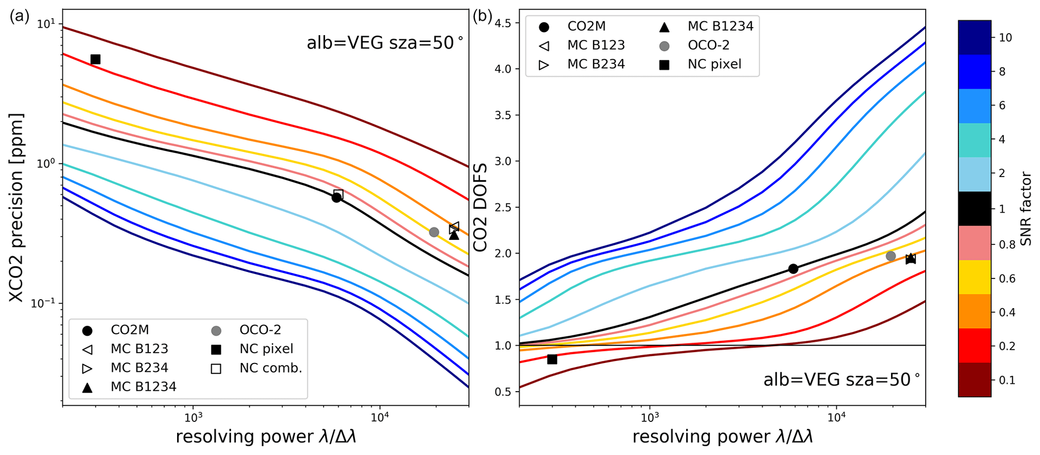
Figure 3 $X_{{\mathrm{CO}}_{\mathrm{2}}}$ precision (a) and corresponding degrees of freedom for CO₂ (b) of the fictitious CVAR instrument for a resolving power $\mathit{\lambda }/\mathrm{\Delta }\mathit{\lambda }$ that evolves from 200 to 30 000 (horizontal axis) and for an SNR that evolves from 0.1 to 10 times the CO₂M reference SNR (colour scale) for the situation VEG-50°. Symbols give the same quantities for NanoCarb (NC; squares), MicroCarb (MC; triangles for various band combinations), CO₂M (black circles) and OCO-2 (grey circles). It should be noted that NanoCarb does not have a spectral resolution per se; the resolving powers used to plot its performance were solely chosen for the sake of comparing the performance of NanoCarb and CVAR.

4.1.1 $X_{{\mathrm{CO}}_{\mathrm{2}}}$ precision and degrees of freedom

Here, we assess the impact of varying the spectral resolution and signal-to-noise ratio. For the atmospheric situation VEG-50°, Fig. 3 shows the $X_{{\mathrm{CO}}_{\mathrm{2}}}$ precision (or random error) and degrees of freedom (hereafter DOFs) as a function of both the resolving power $\mathit{\lambda }/\mathrm{\Delta }\mathit{\lambda }$ and the signal-to-noise ratio (SNR) for CVAR and the exact OCO-2, CO₂M, MicroCarb, and NanoCarb concepts (results for exactly defined concepts are discussed in Sect. 5). The random error is computed from the a posteriori covariance matrix $\widehat{\mathbf{S}}$ given in Eq. (2), and the DOFs correspond to the sum of the CO₂-related diagonal elements of matrix A, given in Eq. (3). As the results (i.e. values) change for other albedo models and SZAs but the conclusions do not, figures that include all 12 atmospheric situations are shown in the Supplement.

Results for the reference CO₂M SNR are given by the black line. The $X_{{\mathrm{CO}}_{\mathrm{2}}}$ precision evolves from 1.96 ppm for $\mathit{\lambda }/\mathrm{\Delta }\mathit{\lambda }$ = 200 to 0.16 ppm for $\mathit{\lambda }/\mathrm{\Delta }\mathit{\lambda }$ = 30 000. These values are consistent with those reported by previous studies: Galli et al. (2014) showed that degrading the spectral resolution increased the $X_{{\mathrm{CO}}_{\mathrm{2}}}$ random errors (values cannot be compared because no real measurement is processed here), and Wu et al. (2020) reported an increase in mean $X_{{\mathrm{CO}}_{\mathrm{2}}}$ retrieval noise from 0.25 to 0.59 ppm (compared to an increase from 0.21 to 0.56 ppm in this work) when degrading OCO-2 measurements ($\mathit{\lambda }/\mathrm{\Delta }\mathit{\lambda }$ ∼ 20 000) to CO₂M-like resolving powers ($\mathit{\lambda }/\mathrm{\Delta }\mathit{\lambda }$ ∼ 6000). This improvement in precision with increasing resolving power is correlated to DOFs values that also increase with resolving power from 1.02 to 2.45. Indeed, the more information a measurement can bring, the lower the $X_{{\mathrm{CO}}_{\mathrm{2}}}$ random error. Changing the SNR has similar effects: the less noisy a measurement, the more information it can carry; thus, increasing the SNR increases the DOFs and reduces the $X_{{\mathrm{CO}}_{\mathrm{2}}}$ random error. For example, for $\mathit{\lambda }/\mathrm{\Delta }\mathit{\lambda }$ = 6000 (close to the resolution of CO₂M), the $X_{{\mathrm{CO}}_{\mathrm{2}}}$ precision evolves from 2.34 to 0.11 ppm when multiplying the SNR by 100. Overall, increasing the SNR by 2 orders of magnitude improves the $X_{{\mathrm{CO}}_{\mathrm{2}}}$ precision by a factor ranging from 16 to 37 (for increasing resolving powers), whereas increasing the resolving power by 2.2 orders of magnitude (from $\mathit{\lambda }/\mathrm{\Delta }\mathit{\lambda }$ = 200 to $\mathit{\lambda }/\mathrm{\Delta }\mathit{\lambda }$ = 30 000) only improves the $X_{{\mathrm{CO}}_{\mathrm{2}}}$ precision by a factor ranging from 10 to 23 (for increasing SNR values). Hence, it appears that the $X_{{\mathrm{CO}}_{\mathrm{2}}}$ precision is more sensitive to SNR improvements than to resolving-power improvements for large improvements of 2 orders of magnitude centred on CO₂M instrument characteristics. However, as it can be seen in Fig. 3 (and in Fig. S3), this conclusion does not hold for smaller local improvements, which generally result in better $X_{{\mathrm{CO}}_{\mathrm{2}}}$ precision gains through resolving-power improvements than through SNR improvements (see Fig. S3).

Furthermore, the $X_{{\mathrm{CO}}_{\mathrm{2}}}$ precision and DOFs broadly show two slope changes (on a logarithmic scale) as the resolving power $\mathit{\lambda }/\mathrm{\Delta }\mathit{\lambda }$ increases. Depending on the SNR, the first occurs around $\mathit{\lambda }/\mathrm{\Delta }\mathit{\lambda }$ ∼ 400–1000. It corresponds to the complete P-R spectral band structure becoming visible, as previously mentioned in relation to Fig. 2. Then, the second slope change occurs around $\mathit{\lambda }/\mathrm{\Delta }\mathit{\lambda }$ ∼ 4000–10 000. This corresponds to the individual spectral lines of CO₂ becoming clearly visible in spectral band branches, as also mentioned in relation to Fig. 2. Between these two slope changes ($\mathit{\lambda }/\mathrm{\Delta }\mathit{\lambda }$ ∼ 1000–4000), improvements in resolving power are less efficient at improving $X_{{\mathrm{CO}}_{\mathrm{2}}}$ precision than they are elsewhere along the resolving-power dimension (see Fig. S3). This explains why, for the large (2 orders of magnitude) improvements in resolving power and SNR explored in this study, the SNR has a larger impact on precision than the resolving power. This result also underlines the critical importance of resolving new spectral features (the P-R band structure below $\mathit{\lambda }/\mathrm{\Delta }\mathit{\lambda }$ ∼ 1000 or the individual spectral lines above $\mathit{\lambda }/\mathrm{\Delta }\mathit{\lambda }$ ∼ 4000) to gain $X_{{\mathrm{CO}}_{\mathrm{2}}}$ precision efficiently.

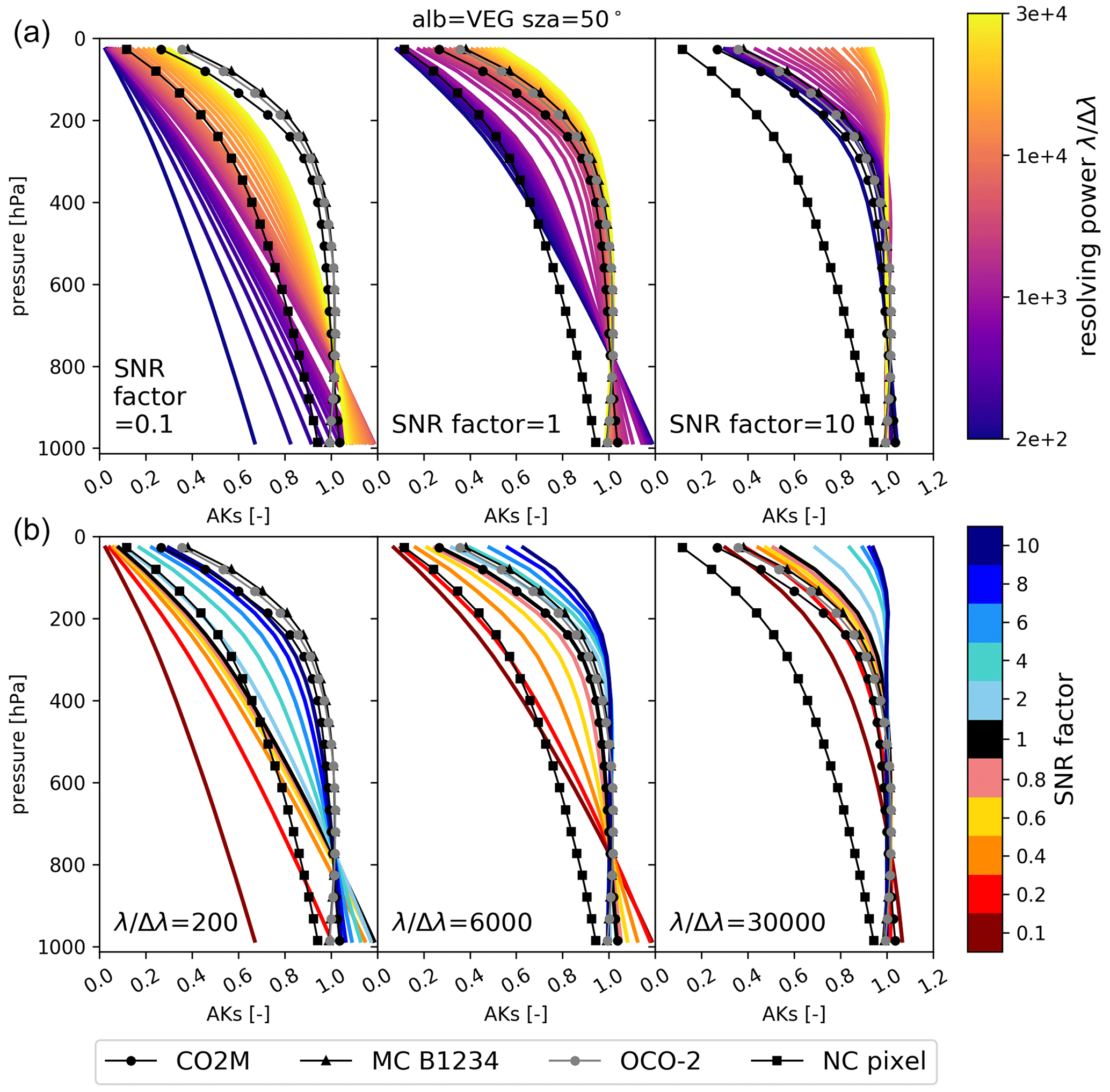
Figure 4 Vertical sensitivities (AKs) (a) as a function of resolving power $\mathit{\lambda }/\mathrm{\Delta }\mathit{\lambda }$ for three different SNR scaling factors and (b) as a function of SNR for three different resolving powers $\mathit{\lambda }/\mathrm{\Delta }\mathit{\lambda }$ for the observational situation VEG-50°. Black lines with symbols give the vertical sensitivities for CO₂M (black circles), MicroCarb (triangles), NanoCarb (squares) and OCO-2 (grey circles).

In addition, we note that these slope changes do not occur at the exact same resolving power for different SNR values, and they vary in sharpness. Indeed, the increase in spectral resolution only brings more information if the band structure and spectral lines, which become progressively visible, are significant with respect to the noise level. We note that these slope changes occur for smaller resolving powers as SNR increases and that the DOFs and $X_{{\mathrm{CO}}_{\mathrm{2}}}$ precision results for a high SNR and low resolving powers correspond to the results for a low SNR and high resolving powers. Thus, there is a broad symmetry in the impact of the SNR and resolving power on $X_{{\mathrm{CO}}_{\mathrm{2}}}$ retrieval performance.

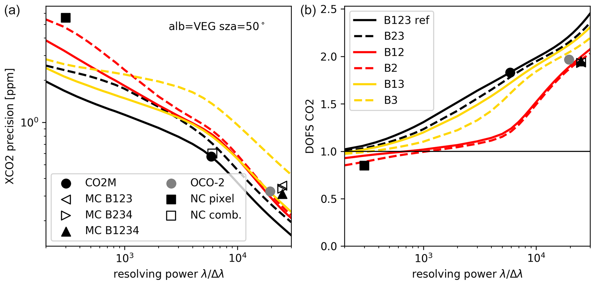
Figure 5 $X_{{\mathrm{CO}}_{\mathrm{2}}}$ precision (a) and corresponding degrees of freedom for CO₂ (b) of the fictitious CVAR instrument for a resolving power $\mathit{\lambda }/\mathrm{\Delta }\mathit{\lambda }$ that evolves from 200 to 30 000 (horizontal axis) and for different spectral band selections: with and without the O₂ 0.76 µm band (B1; solid and dashed lines, respectively), with both the CO₂ 1.6 and 2.05 µm bands (B23; black), with only the 1.6 µm band (B2; red), and with only the 2.05 µm band (B3; yellow) for the situation VEG-50°. Symbols give the same quantities for NanoCarb (NC; squares), MicroCarb (MC; triangles for various band combinations), CO₂M (black circles) and OCO-2 (grey circles). It should be noted that NanoCarb does not have a spectral resolution per se; the resolving powers used to plot its performance were solely chosen for the sake of comparing the performance of NanoCarb and CVAR.

4.1.2 Vertical sensitivity: column averaging kernels

In addition to information content (given by the DOFs and, symmetrically, by the precision), the vertical sensitivity (or column averaging kernels, hereafter denoted AKs) of the $X_{{\mathrm{CO}}_{\mathrm{2}}}$ retrievals must be examined (see Sect. 3.2.1). Taking into account the vertical sensitivity of total columns is especially important when exploiting local column enhancements of vertically inhomogeneous concentration increases. Indeed, any deviation from unity in the vertical sensitivity wrongfully scales differences between the unknown truth and the prior into the retrieved column enhancement, thus calling for a posteriori corrections, as presented by Krings et al. (2011) and also included by Borchardt et al. (2021) for aircraft observation processing. Figure 4 shows AKs for CVAR with a resolving power varying from $\mathit{\lambda }/\mathrm{\Delta }\mathit{\lambda }$ = 200 to 30 000 and for three different scaling factors of the CO₂M noise model (top row). It conversely also shows AKs for scaling factors of the CO₂M noise model that vary from 0.1 to 10 and for three different resolving powers (bottom row). Figure 4 only includes results for the situation VEG-50°. Results for the other situations are shown in the Supplement. For low SNR and resolving-power values, the AKs reach their maximum in the atmospheric layer closest to the ground and have near-zero values at the top of the atmosphere. As the SNR or resolving power (or both) increase, the sensitivities for layers close to the ground improve and become higher than 1. For noise levels and a resolving power of about 6000 and above, the vertical sensitivity values are close to 1 from the ground surface up to approximately 300 hPa and then decrease. For even higher SNR and resolving power values, the AKs converge towards 1 for all atmospheric layers. Thus, just as for their impact on the $X_{{\mathrm{CO}}_{\mathrm{2}}}$ precision or DOFs, the resolving power and noise level of an observing concept have very similar impacts on the AK shape for CVAR.

4.2 Impact of spectral resolution and spectral band selection

This subsection explores the combined impact of spectral resolution and band selection on $X_{{\mathrm{CO}}_{\mathrm{2}}}$ retrieval performance. First, we discuss how the $X_{{\mathrm{CO}}_{\mathrm{2}}}$ precision and CO₂ and non-CO₂-related degrees of freedom evolve with spectral resolution and band selection, and then we examine $X_{{\mathrm{CO}}_{\mathrm{2}}}$ vertical sensitivities. Finally, we explore the sensitivity of $X_{{\mathrm{CO}}_{\mathrm{2}}}$ to a priori misknowledge of interfering geophysical variables, with an eventual focus on aerosol-related parameters.

4.2.1 $X_{{\mathrm{CO}}_{\mathrm{2}}}$ precision and degrees of freedom for CO₂ and interfering geophysical variables

Here, we assess the impact of varying the spectral resolution and band selection. For the atmospheric situation VEG-50° (results for other situations are given in the Supplement), Fig. 5 shows the $X_{{\mathrm{CO}}_{\mathrm{2}}}$ precision and DOFs as a function of both the resolving power $\mathit{\lambda }/\mathrm{\Delta }\mathit{\lambda }$ and spectral band selection for CVAR (with SNR fixed at its reference value) for the exact OCO-2, CO₂M, MicroCarb and NanoCarb concepts (results for exactly defined concepts are discussed in Sect. 5). We first note that including the O₂ 0.76 µm band (denoted B1 in Fig. 5) increases the CO₂ DOFs for CVAR cases compared to cases where it is not included (denoted B2, B3 and B23 in Fig. 5). This spectral band is indeed sensitive to surface pressure, temperature and aerosols and can thus bring independent constraints on these geophysical parameters that show sensitivities that correlate with the CO₂ sensitivity of the 1.6 and 2.05 µm bands. For resolving powers above 1000, adding the O₂ 0.76 µm band has less of an impact on the $X_{{\mathrm{CO}}_{\mathrm{2}}}$ precision for the B2 than for the B3 cases. This may be explained by the fact that spectral lines are more saturated at B3, so it provides less information regarding the length of the optical path than B2 does. We can also notice that the CO₂ DOFs for B3 and B13 are always higher than those for the B2 and B12 cases. This may be explained by the fact that the CO₂M 2.05 µm band includes two full sets of CO₂ P-R absorption branches (out of the three present near 2.05 µm, with one more saturated than the other, see Fig. 1), whereas there is only one set of CO₂ branches in B2 near 1.6 µm, for identical SNR values between B2 and B3. Thus, B3 carries more CO₂ information than B2. Interestingly, we can also notice that band configurations with higher DOFs do not systematically translate into better $X_{{\mathrm{CO}}_{\mathrm{2}}}$ precision: for example, B3 and B13 always show higher DOFs than B2 and B12 but very similar $X_{{\mathrm{CO}}_{\mathrm{2}}}$ precisions to them from $\mathit{\lambda }/\mathrm{\Delta }\mathit{\lambda }=$3000 and upwards. This is due to the covariance between CO₂ elements in the state vector that vary between band selection cases (see Fig. S18), which shows that different spectral bands carry different CO₂ information.

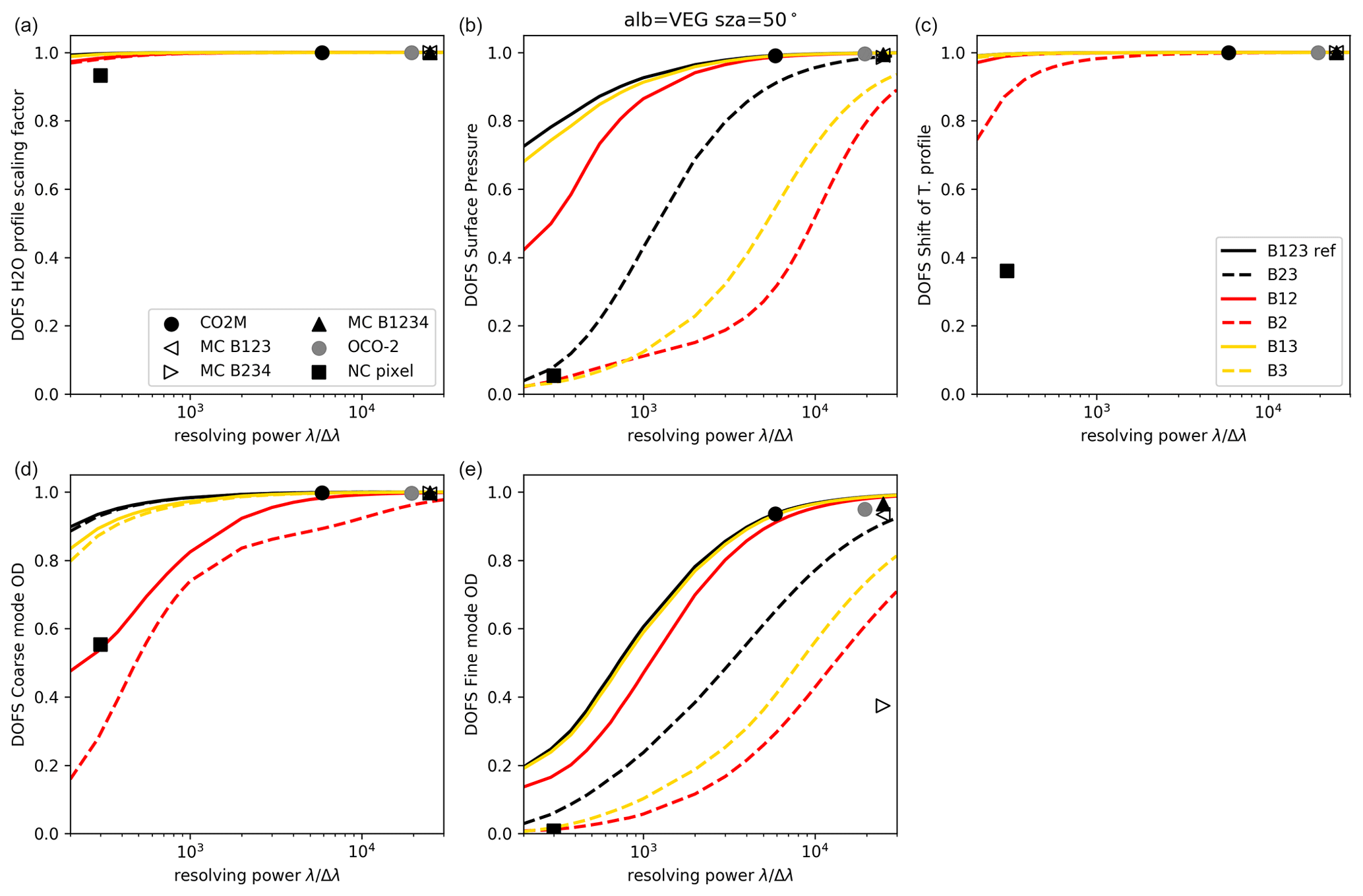
Figure 6 Degrees of freedom for the H₂O scaling factor (a), surface pressure (b), temperature profile shift (c), coarse-mode aerosol optical depth (d) and fine-mode aerosol optical depth (e) for the fictitious CVAR instrument with a resolving power $\mathit{\lambda }/\mathrm{\Delta }\mathit{\lambda }$ that evolves from 200 to 30 000 (horizontal axis) and for different spectral band selections: with and without the O₂ 0.76 µm band (B1; solid and dashed lines, respectively), with both the CO₂ 1.6 and 2.05 µm bands (B23; black), with only the 1.6 µm band (B2; red), and with only the 2.05 µm band (B3; yellow) for the situation VEG-50°. Symbols give the same quantities for NanoCarb (NC; squares), MicroCarb (MC; triangles for various band combinations), CO₂M (black circles) and OCO-2 (grey circles). It should be noted that NanoCarb does not have a spectral resolution per se; the resolving powers used to plot its performance were solely chosen for the sake of comparing the performance of NanoCarb and CVAR.

For the atmospheric situation VEG-50° (results for other situations are given in the Supplement), Fig. 6 completes Fig. 5 by showing the DOFs for interfering geophysical variables (H₂O profile scaling factor, surface pressure, temperature profile shift and aerosol optical depths; albedo-related parameters are not included because they are all very close or equal to 1) as a function of both the resolving power $\mathit{\lambda }/\mathrm{\Delta }\mathit{\lambda }$ and spectral band selection for CVAR (with the SNR fixed at its reference value) and the exact OCO-2, CO₂M, MicroCarb and NanoCarb concepts (see Sect. 5). For all five variables, the DOFs increase with resolving power and tend towards 1. The H₂O profile scaling factor and temperature profile shift exhibit high (close to 1) DOFs for almost all resolving powers and spectral band selection cases in the configuration used here. Surface pressure and aerosol optical depths (variables that influence the length of the optical path) have more sensitivity to the resolving power and, especially, to the inclusion – or not – of the O₂ 0.76 µm band (B1) in the spectral band selection. Cases that do not include B1 show much lower DOFs for these variables, illustrating once again how useful this band is for constraining interfering geophysical variables. This result is made possible by the usual (see the OCO-2 processing algorithm ACOS, for example; O'Dell et al., 2018) hypothesis of fixed aerosol optical properties, which enables the sharing of optical path information across spectral bands. Overall, we can also note that, for all geophysical variables, the DOFs for B13 are more or less significantly closer to those of B123 compared to the DOFs of B12. This shows that the CO₂ 1.6 µm band brings only a little complementary interfering variable information on the top of that already carried by the 2.05 µm band.

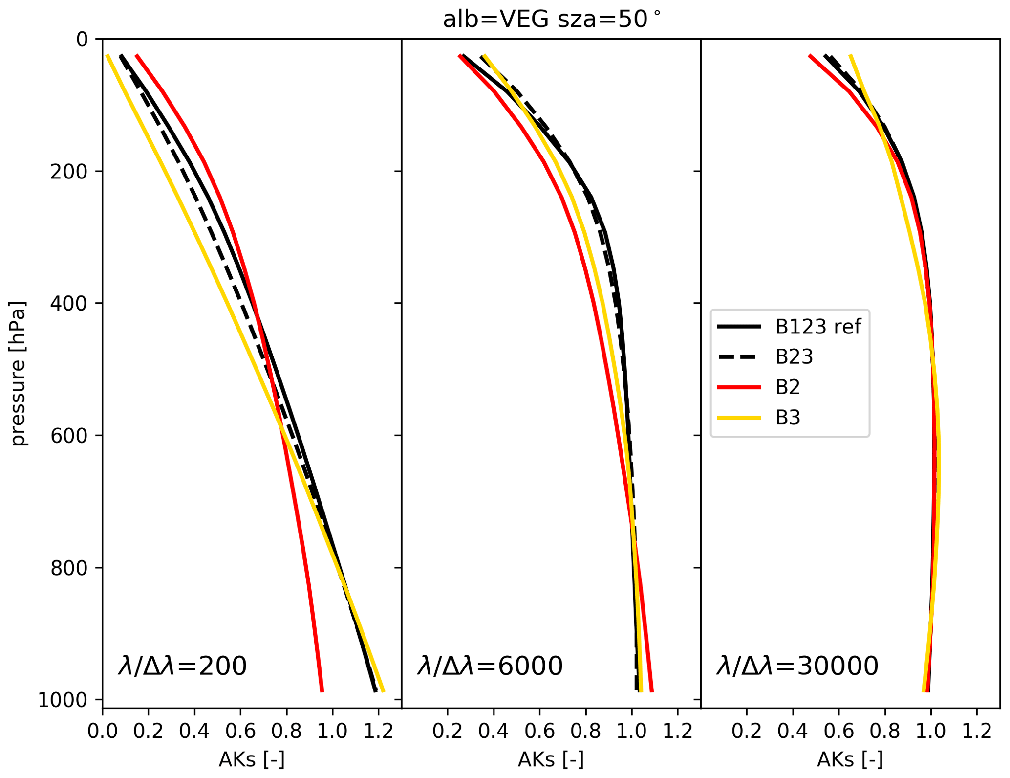
Figure 7 Vertical sensitivities (AKs) for different spectral band selections (for explanations of the line colours and styles, see the legend) and three different resolving powers $\mathit{\lambda }/\mathrm{\Delta }\mathit{\lambda }$ for the observational situation VEG-50°.

Previous studies that have explored the impact of spectral band selection and/or the spectral resolution on $X_{{\mathrm{CO}}_{\mathrm{2}}}$ performance provide conclusions that are in broad agreement with the previously presented results. Wilzewski et al. (2020) studied the performance of $X_{{\mathrm{CO}}_{\mathrm{2}}}$ retrievals from spectrally degraded GOSAT measurements using the 1.6 or 2.05 µm spectral band only. While the methodologies are hardly comparable (because this study is only based on synthetic simulations), both works agree that the trend of $X_{{\mathrm{CO}}_{\mathrm{2}}}$ precision against resolving power changes around $\mathit{\lambda }/\mathrm{\Delta }\mathit{\lambda }$ = 1000–2000 when solely using the 1.6 or 2.05 µm CO₂ band (see Fig. S11, which shows Fig. 5 plotted on a linear scale). Building on Wilzewski et al. (2020), Strandgren et al. (2020) select the 2.05 µm CO₂ band for the design of a moderate-resolution instrument, partly because it shows scattering particle sensitivity. The results presented here are consistent with the conclusion that using only the 2.05 µm band yields higher DOFs (or the same DOFs for surface pressure at low resolving powers) for all geophysical variables compared to when only the 1.6 µm CO₂ band is used.

4.2.2 Vertical sensitivity: column averaging kernels

Figure 7 gives the column averaging kernel – which describes the $X_{{\mathrm{CO}}_{\mathrm{2}}}$ vertical sensitivity – for all CVAR spectral band selection cases and for three different resolving-power values (200, 6000 and 30 000). For lower resolving powers, spectral band selection cases that include the CO₂ 2.05 µm band (B3) show a greater sensitivity to atmospheric levels close to the surface. This may be explained by the fact that this spectral band includes saturated spectral lines which are more sensitive to CO₂ concentration variations in atmospheric layers close to the surface, as it can be seen for example in Fig. 2 in Roche et al. (2021). As seen in Fig. 4, AKs tend to converge towards unity as the resolving power increases, and this difference between bands disappears. Besides, if we compare the AKs for the B23 and B123 spectral band selection cases, we note that including an O₂-sensitive band does not have a strong impact on the $X_{{\mathrm{CO}}_{\mathrm{2}}}$ vertical sensitivity.

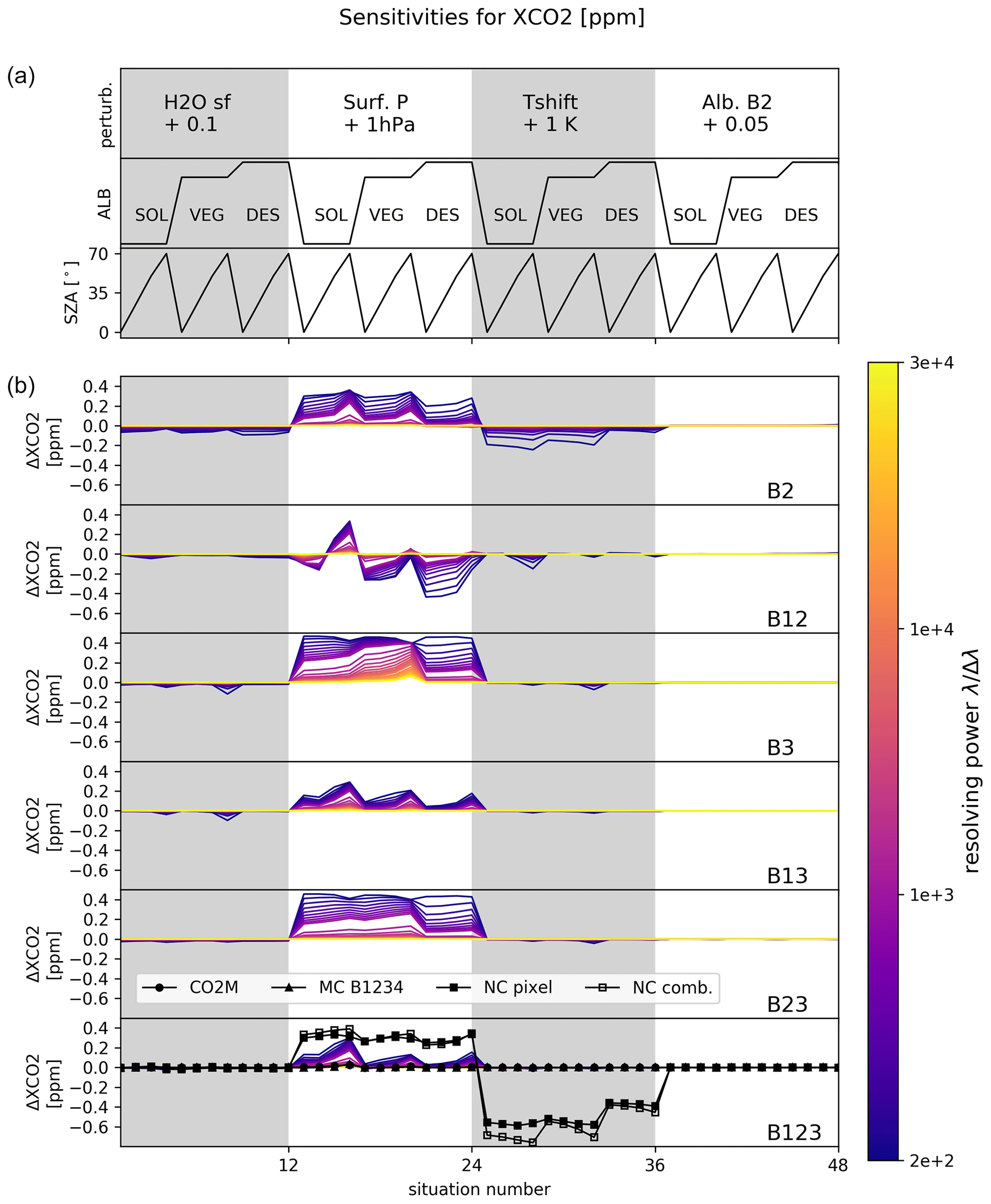
Figure 8 $X_{{\mathrm{CO}}_{\mathrm{2}}}$ sensitivities (denoted $\mathrm{\Delta }{X}_{{\mathrm{CO}}_{\mathrm{2}}}$) to prior misknowledge of the water vapour, surface pressure, temperature profile shift and 1.6 µm band albedo value (perturb., described in the top panel) for 12 observational situations (ALB and SZA, described in the second and third panels), six different CVAR spectral band selections (lines in the six bottom panels) and resolving-power values ranging from 200 to 30 000 (colour scale). Black lines with symbols give the same sensitivities for CO₂M (circles), MicroCarb (triangles) and NanoCarb (squares) in the bottom panels (B2, B12, B3, B13, B23 and B123; b).

4.2.3 Geophysical information entanglements

Geophysical information is entangled in SWIR measurements (as illustrated for example by the a posteriori correlation matrices shown in Fig. S18 or in Fig. 10) to an extent that depends on the measurement nature (spectrum or truncated interferogram) and its characteristics (spectral band selection, spectral resolution, SNR, etc.). One consequence of these entanglements is that possible a priori misknowledge of the atmospheric state can impact the retrieved $X_{{\mathrm{CO}}_{\mathrm{2}}}$ and cause biases; this is called smoothing error (Connor et al., 2008; Rodgers, 2000). In this section, we use the averaging kernel matrix A to propagate a priori misknowledge of the synthetic true state of the atmosphere for non-CO₂ interfering variables in order to evaluate its impact on the retrieved $X_{{\mathrm{CO}}_{\mathrm{2}}}$. Figure 8 shows, for the 12 atmospheric and observational situations considered in this work, the impact on $X_{{\mathrm{CO}}_{\mathrm{2}}}$ of a priori misknowledge of several state vector variables for all CVAR spectral band selection cases, for resolving-power values ranging from 200 to 30 000, and for the exact MicroCarb, CO₂M and NanoCarb concepts (see Sect. 5 for the exactly defined concepts). These a priori perturbations include (1) +10 % to the H₂O profile scaling factor, (2) + 1 hPa to the surface pressure, (3) + 1 K to the temperature profile shift, and (4) +0.05 to the albedo in the 1.6 µm band. All situations and perturbations are sorted along a unique axis, and Fig. 8a describes both the situations (albedo and SZA) and the perturbations considered.

First, regarding water vapour, the $X_{{\mathrm{CO}}_{\mathrm{2}}}$ sensitivity is very small for all CVAR band selection configurations (consistent with the results in Fig. 6), spectral resolutions and exactly described concepts: it amounts to a maximum of 0.12 ppm in absolute value for VEG-70° in the CVAR B3 case for the lowest resolving power. This means that if a water vapour plume is correlated with a CO₂ emission plume (in the exhaust fumes of a coal-fired power plant, for instance), a small bias in the retrieved $X_{{\mathrm{CO}}_{\mathrm{2}}}$ enhancement could then hamper estimations from an instrument with low resolving power (but, potentially, high spatial resolution). However, considering that emission rates computed from enhancements with mass-balance approaches may have uncertainties of up to 65 % (mainly due to wind-speed errors; Varon et al., 2018), this sensitivity of the retrieved $X_{{\mathrm{CO}}_{\mathrm{2}}}$ to water vapour appears insignificant.

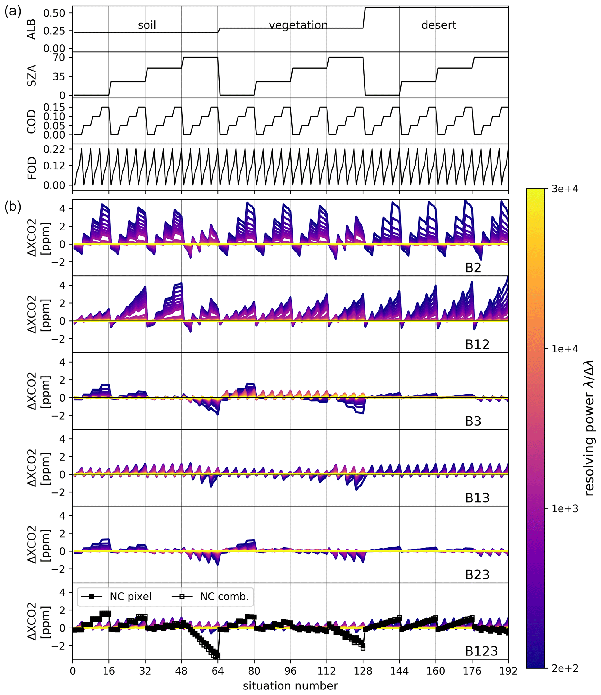
Figure 9 $X_{{\mathrm{CO}}_{\mathrm{2}}}$ sensitivities (denoted $\mathrm{\Delta }{X}_{{\mathrm{CO}}_{\mathrm{2}}}$) to prior misknowledge of aerosol optical depths (COD and FOD, described in the third and fourth top panels) for 12 observational situations (ALB and SZA, described in first and second top panels), six different CVAR spectral band selections (B2, B12, B3, B13, B23 and B123; lines in the bottom six panels;  b) and resolving-power values ranging from 200 to 30 000 (colour scale). Black lines with symbols (squares) in the bottom panel (B123; b) give the same sensitivities for NanoCarb (line B123).

Regarding surface pressure, the $X_{{\mathrm{CO}}_{\mathrm{2}}}$ sensitivities are close to zero for all resolving powers above 10 000 and increase differently depending on the spectral band selection case for lower resolving powers. They reach up to 0.47 ppm for the CVAR B3 case at the lowest resolving-power value tested. Overall, the sensitivity of $X_{{\mathrm{CO}}_{\mathrm{2}}}$ to prior surface pressure misknowledge is reduced when the O₂ 0.76 µm band is included in the measurement, consistent with the results shown in Fig. 6. These sensitivities can be expected to impact the full swath of an imaging instrument with lower resolving powers and can thus be removed when computing an enhancement. However, they would blindly impact observations without emission plumes to detect, thus making these observations hard to exploit for other purposes than anthropogenic point-source monitoring.

Regarding the temperature profile global shift, consistent with the high DOFs shown in Fig. 6, the $X_{{\mathrm{CO}}_{\mathrm{2}}}$ sensitivities are very small overall for spectral resolving powers above 1000 and for all CVAR spectral band selection cases. For resolving powers lower than 1000, they can reach up to 0.23 ppm in absolute value (for the CVAR B2 case, for instance; see the lower DOFs in Fig. 7).

Finally, all cases and concepts exhibit near-zero $X_{{\mathrm{CO}}_{\mathrm{2}}}$ sensitivities (or even, by construction, exactly zero $X_{{\mathrm{CO}}_{\mathrm{2}}}$ sensitivities for the CVAR B3 and B13 cases) when the 1.6 µm CO₂ band albedo is perturbed by 0.05. This reflects the albedo DOFs (which are very close or equal to 1) that we obtain with this inverse setup configuration as well as the low posterior correlations between albedo and CO₂ parameters in the state vector.

4.2.4 Focus on sensitivities to prior aerosol misknowledge

We follow the approach used for NanoCarb performance assessment (Dogniaux et al., 2022), which was first introduced by Buchwitz et al. (2013) for the performance assessment of CarbonSat. Considering the 12 previously described atmospheric and observational situations that span three different albedo models and four SZA values, we explore the $X_{{\mathrm{CO}}_{\mathrm{2}}}$ sensitivities for synthetic coarse-mode aerosol optical depths spanning 0.001–0.15 (with a fixed prior of 0.02) and fine-mode aerosol optical depths spanning 0.001–0.22 (with a fixed prior of 0.05), thus yielding 192 situations in total. This a priori misknowledge of aerosol optical depths is propagated through the averaging kernel matrix A to evaluate its impact on retrieved $X_{{\mathrm{CO}}_{\mathrm{2}}}$ values.

Figure 9 shows, for the 192 considered situations, the impact of a priori aerosol optical depth misknowledge on $X_{{\mathrm{CO}}_{\mathrm{2}}}$ for all CVAR spectral band selection cases, for resolving-power values ranging from 200 to 30 000, and for the exact NanoCarb concept (results for NanoCarb are discussed in Sect. 5). All situations are sorted along a unique axis, and the top four panels in Fig. 9a (ALB, SZA, COD and FOD) describe the given situation (in terms of albedo, SZA, and coarse- and fine-mode optical depths).

For the CVAR B2 and B12 cases, the $X_{{\mathrm{CO}}_{\mathrm{2}}}$ sensitivities at low resolving powers reach up to about ∼ 5 ppm. They correlate mostly to a priori misknowledge of the coarse-mode aerosol optical depth and secondarily to a priori misknowledge of the fine-mode aerosol optical depth, and they diminish as the spectral resolving power increases. Sensitivities also depend on the albedo model and SZA value, thus reflecting that the information content carried by a given measurement also depends on the scene (see the DOFs for all situations in the Supplement). Including the O₂ 0.76 µm band in addition to the CO₂ 1.6 µm band reduces the $X_{{\mathrm{CO}}_{\mathrm{2}}}$ sensitivity to a priori aerosol misknowledge at low SZA values for low resolving powers, but it has a low or even a detrimental impact at higher SZAs.

Unlike the CO₂ 1.6 µm band, the CO₂ 2.05 µm band carries more aerosol information, and thus the results for the CVAR B3 and B13 selection cases show lower impacts of these variables on $X_{{\mathrm{CO}}_{\mathrm{2}}}$ retrievals, with a maximum of ∼ 2 ppm in absolute value. For the CVAR B3 case, the $X_{{\mathrm{CO}}_{\mathrm{2}}}$ sensitivities to a priori aerosol misknowledge are mostly correlated to coarse-mode misknowledge for low resolving powers and to fine-mode misknowledge for higher resolving powers, and they converge towards near-zero values for the highest resolving powers. Interestingly, including the O₂ 0.76 µm band changes this correlation pattern, and the $X_{{\mathrm{CO}}_{\mathrm{2}}}$ sensitivities appear to be mostly correlated to fine-mode aerosol misknowledge in the B13 case, with slightly higher $X_{{\mathrm{CO}}_{\mathrm{2}}}$ sensitivities compared to the B3 case seen in some situations, such as in those with a soil-like or desert-like albedo.

Results for B23 and B123 mostly follow the patterns seen in the B3 and B13 cases (as B3 brings more aerosol information compared to B2) but with slightly lower $X_{{\mathrm{CO}}_{\mathrm{2}}}$ sensitivity values, reflecting the scant complementary information added by B2 on top of B3.

5 Results and discussion for exactly defined concepts: OCO-2, CO₂M, MicroCarb and NanoCarb

5.1 $X_{{\mathrm{CO}}_{\mathrm{2}}}$ precision and degrees of freedom

Besides the results for CVAR, Fig. 3 also includes the performance computed for four explicit concepts: the currently flying OCO-2 and upcoming CO₂M and MicroCarb missions as well as the NanoCarb concept that is currently being studied. First, OCO-2 shows a noise-only-related precision of 0.32 ppm, corresponding to 1.97 DOFs for CO₂-related parameters. The OCO-2 results that we obtain are consistent overall with ACOS results for soundings, with close albedo values per band (see Fig. S6). Also, land nadir OCO-2 $X_{{\mathrm{CO}}_{\mathrm{2}}}$ retrievals show an overall standard deviation of 0.77 ppm compared to the Total Carbon Column Observing Network (TCCON) validation reference (Taylor et al., 2023). This difference with respect to the theoretical uncertainty computed from optimal estimation stems from all the forward and inverse modelling errors that are not accounted for in the retrieval scheme. Thus, this illustrates that the results provided in this study are a lower bound on the actual precisions that these upcoming concepts will have. CO₂M shows an $X_{{\mathrm{CO}}_{\mathrm{2}}}$ precision of 0.56 ppm, which is consistent with the 0.7 ppm precision requirement for a vegetation scene with SZA = 50° given in Meijer and Earth and Mission Science Division (2020). For MicroCarb (MC1234 when including the four spectral bands), we find an $X_{{\mathrm{CO}}_{\mathrm{2}}}$ precision of 0.31 ppm, which satisfactorily compares to the median 0.35 ppm contribution of the SNR to the mission error budget (with the full range of possible contributions being 0.15–0.94 ppm, Denis Jouglet, personal communication, 2021). Also, we can notice that removing one of the two O₂-sensitive spectral bands from MicroCarb measurements (i.e. we consider MC123, which includes the 0.76, 1.6 and 2.05 µm bands, and MC234, which includes the 1.6, 2.05 and 1.27 µm bands) slightly decreases the precision. Indeed, less geophysical information is available to help constrain interfering variables. Finally, MicroCarb (MC1234) shows only slightly higher CO₂ DOFs compared to CO₂M despite having a spectral resolution that is 5 times higher. This may be explained by the fact that their respective spectral bands do not cover the same wavelength intervals, as can be seen in Fig. 1.

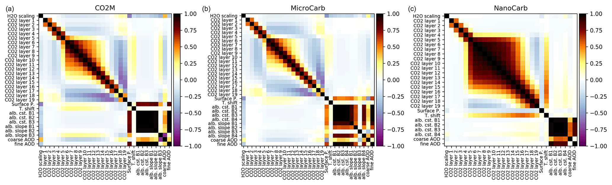
Figure 10 A posteriori correlation matrices for CO₂M (a), MicroCarb (b) and NanoCarb (c) for the VEG-50° situation.

Two different $X_{{\mathrm{CO}}_{\mathrm{2}}}$ precision results are included for NanoCarb in Fig. 3: one for a unique pixel located at the FOV centre (filled square) and another obtained after combining results acquired from different viewing angles as the two-dimensional FOV of NanoCarb flies over a scene (see Sect. 2.3 or the extensive description in Dogniaux et al., 2022). For a single observation of a given scene performed by the central pixel in the FOV, NanoCarb yields a precision of 5.6 ppm. However, after combining the maximum number of observations (102, over different viewing angles) of the same scene, the NanoCarb random error is reduced to 0.60 ppm, which is close to the performance of CO₂M. It must be noted that, because of its very nature, NanoCarb does not have a spectral resolution per se. Thus, we arbitrarily attributed a resolving power of $\mathit{\lambda }/\mathrm{\Delta }\mathit{\lambda }$ = 300 to plot the pixel-wise performance of NanoCarb and a resolving power of $\mathit{\lambda }/\mathrm{\Delta }\mathit{\lambda }$ = 6000 to plot the performance of NanoCarb for combined pixels. This choice enables us to highlight that the pixel-wise performance of NanoCarb is comparable to concepts that measure spectra at low spectral resolution and with low SNR, whereas when the retrieval results from observations that are assumed independent are combined, the $X_{{\mathrm{CO}}_{\mathrm{2}}}$ precision becomes comparable to that of CO₂M.

However, despite their similar precisions, further comparisons enable us to show how their respective $X_{{\mathrm{CO}}_{\mathrm{2}}}$ observations are not equivalent. Indeed, we first notice that their respective DOFs are not comparable at all: CO₂M shows 1.83 DOFs for CO₂, whereas the pixel-wise CO₂ DOFs of NanoCarb amount to 0.85 (no averaging kernel matrix is computed for the NanoCarb combined-pixel results, as performance is evaluated per pixel and they are assumed to be independent when combined). These low CO₂ DOFs for NanoCarb are explained by the low CO₂ information content of NanoCarb measurements (compared to concepts that measure spectra) and its entanglement with other geophysical-variable information, as mentioned in Dogniaux et al. (2022). One can indeed notice that the partial derivatives of CO₂ and other variables are correlated (see Fig. S2): this makes it harder for OE to yield independent estimates for CO₂ and other parameters.

Another way to look at this issue is to consider a posteriori correlations between state vector parameters, as given by the a posteriori covariance matrix $\widehat{\mathbf{S}}$. Pearson correlation coefficient matrices computed from $\widehat{\mathbf{S}}$ are shown for CO₂M, MicroCarb (MC1234) and NanoCarb in Fig. 10. First, regarding the CO₂ profile, we notice the very high positive correlation between different atmospheric layers for NanoCarb compared to the CO₂M and MicroCarb cases. This is a result of the low CO₂ information content in NanoCarb measurements compared to CO₂M and MicroCarb. Also, in this state vector configuration, the NanoCarb a posteriori covariance matrix shows a stronger correlation between CO₂ atmospheric layers and the temperature profile shift than seen for CO₂M and MicroCarb. A slight positive correlation between CO₂ atmospheric layers and albedo parameters can also be noted for NanoCarb, unlike for CO₂M and MicroCarb, which show small negative correlations. The correlation (which has a value of close to 1.0) between albedo parameters of different bands is due to the presence of aerosol optical depth parameters in the state vector (assuming fixed aerosol optical properties). When aerosol optical depths are removed from the state vector, these correlations between albedo parameters of different bands decrease (see Fig. S19). Interestingly, in that case, the correlations between CO₂ atmospheric layers and albedo parameters reach up to 0.6 for NanoCarb, whereas they reach 0.2 and 0.1 for CO₂M and MicroCarb, respectively (see the Supplement). Thus, all things considered, NanoCarb contains less geophysical information than other concepts that measure spectra, and such a comparison helps pave the way for future improvement of the NanoCarb concept.

5.2 Vertical sensitivity: column averaging kernels

Besides the results for CVAR, Fig. 4 also includes the vertical sensitivities of OCO-2, CO₂M, MicroCarb and NanoCarb. Thanks to their spectral resolutions and SNRs, CO₂M and MicroCarb show vertical sensitivities that are close to 1 from the surface to about 300 hPa and then decrease. Interestingly, NanoCarb AKs do not have exactly the same shape as the CVAR, CO₂M or MicroCarb AKs. For the atmospheric layers closest to the ground, the NanoCarb AK follows the AK shape of an instrument with low resolving power and a low SNR (consistent with how the NanoCarb single-pixel performance compares to CVAR in Fig. 3). For higher atmospheric layers, it follows the AK shape of an instrument with medium resolving power and a low SNR or vice versa.

5.3 Non-CO₂ degrees of freedom

Besides the results for CVAR, Fig. 6 also gives interfering variable DOFs for the exact OCO-2, CO₂M, MicroCarb and NanoCarb concepts. For MicroCarb, OCO-2, and CO₂M, the DOFs for the H₂O profile scaling factor, surface pressure, temperature global shift and coarse-mode aerosol optical depth are all nearly equal to 1. Only for the fine-mode aerosol optical depth do the DOFs appear to be – slightly – lower than 1, with the exception of the MicroCarb B234 configuration test, where the fine-mode DOF is close to 0.4. This shows that different optical path length information is carried depending on whether the O₂ 0.76 µm or 1.27 µm band is used. NanoCarb exhibits near-zero DOFs for surface pressure and fine-mode optical depth in this retrieval configuration as well as non-zero yet rather low DOF values for H₂O profile scaling factor, temperature global shift and coarse-mode aerosol optical depth (0.93, 0.36 and 0.55, respectively). Given how small some of these DOF values are, we also conclude that the state vector used to process NanoCarb measurements should be adjusted to only include the most essential geophysical variables. For example, aerosol optical depths could be removed.

5.4 Geophysical information entanglements

Besides the results for CVAR, Fig. 8 also gives the sensitivities of CO₂M, MicroCarb and NanoCarb $X_{{\mathrm{CO}}_{\mathrm{2}}}$ to a priori misknowledge of the water vapour, surface pressure, temperature profile, and 1.6 µm albedo. These $X_{{\mathrm{CO}}_{\mathrm{2}}}$ sensitivities are close to zero for MicroCarb and CO₂M for the four tested geophysical variables.

Prior misknowledge of the surface pressure reaches up to 0.39 ppm for NanoCarb, again indicating results comparable to low-spectral-resolution instruments. The sensitivities for the NanoCarb central-pixel results (filled squares) and the NanoCarb combined results for the central row of pixels (empty squares) differ slightly because information entanglement evolves depending on the pixel location in the NanoCarb FOV. NanoCarb also shows significant $X_{{\mathrm{CO}}_{\mathrm{2}}}$ sensitivities to a priori temperature misknowledge that reach −0.76 ppm, consistent with the strong correlation shown between the temperature profile shift and CO₂-related parameters in the state vector (see Fig. 10). This result is not surprising as the version of the NanoCarb concept used in this work did not consider the possible impact of entanglements between CO₂ and temperature (see Sect. 2.3 or Dogniaux et al., 2022, Gousset et al., 2019). This paves the way for future improvements of this very compact instrumental concept.

Figure 11 Same as Fig. 10, but only results for CO₂M, MicroCarb and NanoCarb are included.

Regarding the sensitivity to prior aerosol misknowledge, Fig. 9 also shows results for the exact NanoCarb concept: those for both the central pixel in the FOV and the combination of the central along-track row of pixels. For SZA values lower than or equal to 50° in soil and vegetation albedo situations and for all SZAs in desert albedo situations, those mostly correlate with the coarse-mode aerosol misknowledge, reaching absolute values of up to 1.7 ppm. For SZA = 70° in soil and vegetation albedo situations, not only do the NanoCarb aerosol DOFs increase (see Figs. S16 and S17), but correlations between CO₂ and aerosol state variables also increase by a lot (see Fig. S20), thus leading to the larger sensitivities shown in Fig. 9 (or Fig. 11). This illustrates that different surface types and SZAs must be explored for thorough performance assessments.

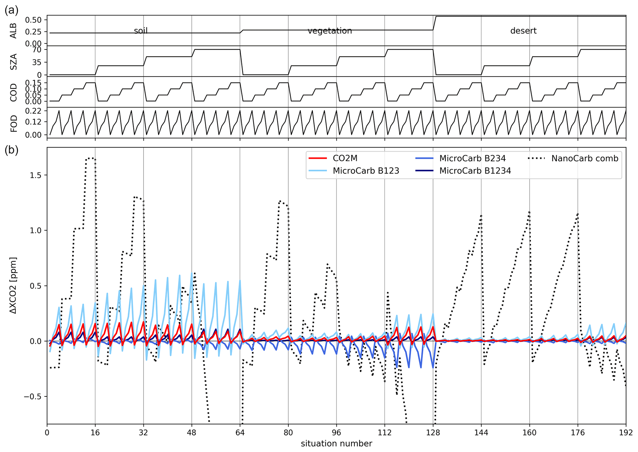
Figure 11 is similar to Fig. 9 but focuses on the exact concepts of CO₂M and MicroCarb studied. Their $X_{{\mathrm{CO}}_{\mathrm{2}}}$ sensitivities to prior aerosol optical depth misknowledge are overly correlated to that of fine-mode optical depth. This can be explained by the fact that their coarse-mode optical depth DOFs are very close to 1, thus enabling the correct estimation (in this synthetic simulation setup) of this geophysical parameter, which results in a very low impact of coarse-mode optical depth misknowledge on $X_{{\mathrm{CO}}_{\mathrm{2}}}$ retrievals. However, their fine-mode DOFs are below 1, thus leading to estimation errors that impact $X_{{\mathrm{CO}}_{\mathrm{2}}}$ retrievals through a posteriori correlations (see Figs. 10 and S19). Overall, CO₂M shows sensitivities of up to 0.2 ppm, with maximums reached for the SOL-25° situation. These values are well below the 0.5 ppm systematic error requirement (Meijer and Earth and Mission Science Division, 2020) and are expected to be reduced even more by using the aerosol observations provided by the multi-angle polarimeter that will fly alongside the CO₂M spectrometers (Rusli et al., 2021). As for MicroCarb, its $X_{{\mathrm{CO}}_{\mathrm{2}}}$ sensitivities to aerosol optical depth misknowledge peak for soil albedo situations at about 0.6 ppm when only the 0.76 µm O₂ band (B123) is included and at 0.1 ppm when both the 0.76 and 1.27 µm O₂ bands are included (B1234), whereas they peak at −0.2 ppm for vegetation albedo situations when only the 1.27 µm O₂ band is available (B234). Interestingly, the sensitivities of MicroCarb B123 and B1234 are positively correlated to the fine-mode aerosol optical depth values, whereas those of MicroCarb B234 are negatively correlated. This illustrates that the O₂ 1.27 µm band carries optical path length information complementary to that carried by the O₂ 0.76 µm band (see also the a posteriori correlation matrices in Fig. S21).

6 Conclusions

In this work, we have carried out a synthetic survey that describes the impact of measurement design choices on $X_{{\mathrm{CO}}_{\mathrm{2}}}$ retrieval performance for shortwave infrared (SWIR) satellite observations. In order to be representative of the wide range of upcoming concept designs, it explored – for a fictitiously varying CO₂M-like instrument – the impact of three different parameters on the measurement: (1) spectral resolution; (2) signal-to-noise ratio (for values spanning 2 orders of magnitude); and (3) spectral band selection. In addition, four exactly defined concepts have been consistently studied: OCO-2, CO₂M, MicroCarb and NanoCarb.

First, the $X_{{\mathrm{CO}}_{\mathrm{2}}}$ precision and CO₂ information content of SWIR measurements improve upon increasing the resolving power and/or the signal-to-noise ratio. For CO₂M-like SNR values, increasing the resolving power by 2.2 orders of magnitude improves the precision by a factor of about 12. For a resolving power of 6000, multiplying the SNR by 100 improves the precision by a factor of about 21. Overall, for these large changes of about 2 orders of magnitude, the precision is found to be more sensitive to SNR improvements than to spectral resolution improvements. However, small-magnitude improvements in resolving power generally yield more $X_{{\mathrm{CO}}_{\mathrm{2}}}$ precision improvements than SNR improvements do, especially when CO₂ spectral lines are resolved. The separate impacts of these two parameters show a broad symmetry in precision as well as in vertical sensitivities: measurements with lower SNR and/or spectral resolution values give more weight to atmospheric layers close to the surface for the retrieved total columns.

The comparison of different spectral band selections included in the SWIR measurement provided two main conclusions. First, including the O₂ 0.76 µm band strongly increases the information content for parameters that impact the optical path length (for all resolving powers) and helps to noticeably reduce the impact of a priori misknowledge of these parameters on retrieved $X_{{\mathrm{CO}}_{\mathrm{2}}}$ values. Secondly, the CO₂ 2.05 µm band (especially for the coarse aerosol mode) carries more information overall than the 1.6 µm band and thus seems more appropriate for concepts that measure a single CO₂-sensitive spectral band, especially at low to mid-level spectral resolution values. These results also highlight how the precise (and accurate to some extent) retrieval of $X_{{\mathrm{CO}}_{\mathrm{2}}}$ from SWIR observations relies on the amount of information carried by these observations. Reducing the spectral resolution and/or the number of spectral bands to improve spatial resolution increases errors. If these are constant over a full image, they may be removed when calculating the local enhancements of $X_{{\mathrm{CO}}_{\mathrm{2}}}$. However, they may still hamper absolute $X_{{\mathrm{CO}}_{\mathrm{2}}}$ retrievals in plume-free scenes, thus potentially making these observations barely useful for anything but anthropogenic emissions imaging.

The exact CO₂M, MicroCarb and NanoCarb concepts were studied in addition to the fictitiously varying ones. With a spectral resolution that is about 5-times higher but shorter spectral band intervals, MicroCarb shows slightly higher CO₂ DOFs compared to CO₂M, and its $X_{{\mathrm{CO}}_{\mathrm{2}}}$ precision is lower by a factor ranging from about 1.1 to 1.9, depending on the observational situation. Their vertical sensitivities are very similar, and their DOFs for other interfering variables are mostly very close to 1, with the exception of the fine aerosol mode, for which they show slightly lower values. Also, MicroCarb exhibits varying information content on variables related to the optical path length, depending on whether the 0.76 µm band, the 1.27 µm band or both of these O₂-sensitive bands are included in the calculations. Regarding NanoCarb, which only measures truncated interferograms, not full spectra, its pixel-wise $X_{{\mathrm{CO}}_{\mathrm{2}}}$ performance is comparable in many aspects to the performance of low-spectral-resolution and low-SNR spectra-observing concepts. However, the $X_{{\mathrm{CO}}_{\mathrm{2}}}$ precision obtained after combining several observations of the same location is close to the $X_{{\mathrm{CO}}_{\mathrm{2}}}$ precision of CO₂M. A comparison between NanoCarb DOFs and those of spectra-measuring concepts (regardless of their characteristics) highlights that further improvements of the concept are needed to increase its information content for interfering geophysical variables.

Given its scope, which focused on exploring the impact of concept design parameters on $X_{{\mathrm{CO}}_{\mathrm{2}}}$ retrieval performance, this study could not include all the dimensions of a comprehensive mission performance assessment. For example, the accuracy of $X_{{\mathrm{CO}}_{\mathrm{2}}}$ retrieval has not been studied, and greater variability in the possible atmospheric conditions (different aerosol types, layers, contents, thermodynamical profiles, CO₂ concentration vertical profiles, etc.) could be considered, as is usually done in comprehensive observing system simulation experiments. Also, this work obviously could not explore all possible design parameters (e.g. band-wise variations in spectral sampling ratios, varying wavelength intervals for spectral bands, and combinations of different instruments) that impact $X_{{\mathrm{CO}}_{\mathrm{2}}}$ retrieval performance and their implications for anthropogenic plume imaging. These limitations warrant further studies.

This decade will see a large increase in the spaceborne monitoring of $X_{{\mathrm{CO}}_{\mathrm{2}}}$ by a wide variety of SWIR-observing concepts. This work enabled us to explore three of the most critical parameters, and it has shown how different we can expect the upcoming $X_{{\mathrm{CO}}_{\mathrm{2}}}$ products to be in terms of their respective performance and sensitivities to interfering variables. This hints at the extent of work that will be required to compare, reconcile and cross-calibrate the results produced by so many different satellite concepts, especially if their purpose is to support the independent evaluation of mitigation efforts aiming at Paris Agreement objectives.