Validation of Aeolus L2B products over the tropical Atlantic using radiosondes

Since its launch by the European Space Agency in 2018, the Aeolus satellite has been using the first Doppler wind lidar in space to acquire three-dimensional atmospheric wind profiles around the globe. Especially in the tropics, these observations compensate for the currently limited number of other wind observations, making an assessment of the quality of Aeolus wind products in this region crucial for numerical weather prediction. To evaluate the quality of the Aeolus L2B wind products across the tropical Atlantic Ocean, 20 radiosondes corresponding to Aeolus overpasses were launched from the islands of Sal, Saint Croix, and Puerto Rico during August–September 2021 as part of the Joint Aeolus Tropical Atlantic Campaign. During this period, Aeolus sampled winds within a complex environment with a variety of cloud types in the vicinity of the Intertropical Convergence Zone and aerosol particles from Saharan dust outbreaks. On average, the validation for Aeolus Rayleigh-clear revealed a random error of 3.8–4.3 m s⁻¹ between 2 and 16 km, and 4.3–4.8 m s⁻¹ between 16 and 20 km, with a systematic error of $-\mathrm{0.5}\pm \mathrm{0.2}$ m s⁻¹. For Mie-cloudy, the random error between 2 and 16 km is 1.1–2.3 m s⁻¹ and the systematic error is $-\mathrm{0.9}\pm \mathrm{0.3}$ m s⁻¹. It is therefore concluded that Rayleigh-clear winds do not meet the mission's random error requirement, while Mie winds most likely do not fulfil the mission bias requirement. Below clouds or within dust layers, the quality of Rayleigh-clear observations are degraded when the useful signal is reduced. In these conditions, we also noticed an underestimation of the L2B estimated error. Gross outliers, defined as large deviations from the radiosonde data, but with low error estimates, account for less than 5 % of the data. These outliers appear at all altitudes and under all environmental conditions; however, their root cause remains unknown. Finally, we confirm the presence of an orbital-dependent bias observed with both radiosondes and European Centre for Medium-Range Weather Forecasts model equivalents. The results of this study contribute to a better characterisation of the Aeolus wind product in different atmospheric conditions and provide valuable information for further improvement of the wind retrieval algorithm.

1 Introduction

According to the World Meteorological Organisation (WMO), wind is the most critical atmospheric variable lacking in the current Global Observing System (GOS) (Baker et al., 2014). Especially in the Southern Hemisphere (SH), over the oceans and near equatorial regions, numerical weather prediction (NWP) models require additional wind observations with sufficient coverage in time and space to identify key atmospheric dynamics (Stoffelen et al., 2005; Straume et al., 2020). Before the launch of Aeolus in 2018, satellite wind observations in these regions were only available for a limited number of tropospheric layers and were mainly provided by atmospheric motion vectors (AMVs) estimated from tracking cloud and water vapour features (Bormann et al., 2003; Folger and Weissmann, 2014), or by scatterometer measurements of surface winds (Naderi et al., 1991; Portabella and Stoffelen, 2009). In situ measurements derived from aircraft reports, ground stations, or radiosondes are not globally distributed and lead to a lack of observations in the aforementioned regions.

To address these deficiencies, the European Space Agency (ESA) deployed the Atmospheric Dynamics Mission Aeolus in 2018, the first satellite capable of measuring atmospheric winds around the globe from space with a homogeneous space–time wind coverage and altitude-resolved profiles of up to 30 km height (Reitebuch, 2012). The instrument carries a direct-detection Doppler wind lidar called ALADIN (Atmospheric LAser Doppler INstrument) that emits short ultraviolet (UV) pulses at 355 nm along the line of sight (LOS) of the instrument, perpendicular to the satellite's ground track and oriented 35^∘ off-nadir. The Doppler shift of the backscatter signal is detected by a dual-channel receiver consisting of the following elements: a Fizeau interferometer analysing the Doppler shift of the narrowband particle backscatter signal (cloud droplets and aerosols or ice crystals) using the fringe imaging technique (McKay, 2002), referred to as the “Mie channel”, and a dual Fabry–Pérot interferometer detecting the Doppler-shifted frequency of the Rayleigh–Brillouin backscatter spectrum (air molecules) using the double-edge technique (Flesia and Korb, 1999), called the “Rayleigh channel”. The processing algorithm also distinguishes between retrievals originating from “cloudy” or “clear” atmospheric conditions, resulting in Rayleigh-clear and Mie-cloudy observation types. The two channels complement each other, as Mie-cloudy winds can compensate for gaps in Rayleigh-clear observations, especially in cloudy and aerosol-loaded regions. Various NWP centres have demonstrated the added value of assimilating Aeolus winds through significant improvements in model fields and model background information, especially in tropical regions, the upper tropical troposphere, and the lower stratosphere (Rennie et al., 2021; Martin et al., 2023, 2022; Garrett et al., 2022).

For an optimal use of the Aeolus wind observations in NWP models, an assessment of the data quality is essential. To achieve this, several scientific and technical studies are carried out in the framework of calibration/validation (Cal/Val) activities organised by ESA. For wind validation, several reference products have been used such as ground-based remote sensing observations (Belova et al., 2021; Guo et al., 2021; Iwai et al., 2021; Abril-Gago et al., 2023), in situ measurements (Baars et al., 2020; Chen et al., 2021; Ratynski et al., 2023), airborne measurements (Lux et al., 2020; Witschas et al., 2020; Bedka et al., 2021; Witschas et al., 2022), or NWP model equivalents (Martin et al., 2021; Zuo et al., 2022).

Several anomalies in the Aeolus data have already been detected and improvements in the processing chain and the instrument have been made accordingly. These include the implementation of a bias correction in both channels related to the orbital-dependent temperature variations of ALADIN's M1 mirror (Weiler et al., 2021b) and the correction of “pixel anomalies” (Weiler et al., 2021a), which reduced the systematic and random errors in the Rayleigh channel. One phenomenon that needs further exploration is the sensitivity of Aeolus wind quality to the presence of aerosols and clouds, which impact key parameters such as the signal levels or scattering ratio (SR) used to calculate the horizontal line-of-sight (HLOS) winds and the associated error estimate (EE). The tropical Atlantic during the boreal summer, spanning from West Africa to the Caribbean, is the ideal place to explore these dependencies, with a wide range of atmospheric aerosols (Saharan dust aerosols, sea salt aerosols, biomass combustion aerosols) and convective cloud types associated with the West African Monsoon (WAM) circulation and the Intertropical Convergence Zone (ITCZ).

For this purpose, ESA organised the Joint Aeolus Tropical Atlantic Campaign (JATAC) in the period July–September 2021, which deployed sophisticated airborne lidar instruments over Cabo Verde (German Aerospace Center (DLR), Laboratoire ATmosphères, Milieux, Observations Spatiales (LATMOS)) and the Virgin Islands (National Aeronautics and Space Administration (NASA)) but also ground-based instruments such as radiosondes (KIT, University of Oklahoma, University of Utah) and Doppler lidar systems (Leibniz Institute for Tropospheric Research (TROPOS), National Observatory of Athens (NOA)). In this study, we validate Aeolus wind products using radiosondes launched from western Puerto Rico, northern Saint Croix, and Sal Airport on Cabo Verde. The semi-arid island of Sal is located over the tropical East Atlantic off the West African coast, near the northern boundary of the WAM. Rain events are relatively sporadic there, as most synoptic and mesoscale precipitation systems propagate south of the island. The region is exposed to mineral dust plumes emanating from Saharan dust outbreaks. By contrast, the islands of Saint Croix and Puerto Rico are located in the warm and moist Caribbean, where heavy rainfall events and tropical cyclones frequently affect the area. The contribution of the radiosondes in JATAC is complementary to other instruments as they provide accurate wind measurements throughout the troposphere up to the lower stratosphere, which is not probed by many other instruments and provides an almost unique data set for validating the Aeolus winds at this altitude. Furthermore, our approach involves using radiosonde data exclusively from the JATAC campaign to facilitate more comprehensive comparisons with other campaign instruments, considering the scarcity of radiosonde measurements in the tropics, the need for radiosonde launches at local dusk–dawn times to reduce timing gaps and possible variations in Aeolus data quality across different times and locations.

This article is structured as follows: Sect. 2 describes the instruments and data while Sect. 3 details the quality control and co-location criteria used for the validation study. Section 4 deals with the quantification of errors, their dependency on temporal and spatial distance between the compared observations as well as on the presence of clouds and dust. For this purpose, we use the Satellite Application Facility for supporting NoWCasting and very short range forecasting (SAFNWC, Alonso Lasheras et al., 2005) satellite-based meteorological Cloud Type (CT) product and the Copernicus Atmosphere Monitoring Service (CAMS) dust mixing ratio reanalysis. Furthermore, the section includes a case study illustrating the different behaviour of Rayleigh-clear and Mie-cloudy winds under different environmental conditions. Finally, Sect. 5 summarises the main results and provides recommendations for improving the Aeolus wind retrieval algorithm.

2 Instruments and data

2.1 ALADIN and Aeolus wind products

Aeolus is the second Earth Explorer Core mission and measures global atmospheric wind profiles from a 320 km high sun-synchronous dusk–dawn orbit. It carries the ALADIN instrument (Schillinger et al., 2003), which is a direct-detection high-spectral-resolution wind lidar with a Nd:YAG laser transmitter that operates at an ultraviolet wavelength of 354.8 nm. It points at 35^∘ off-nadir with an angle of ∼ 10^∘ from the zonal direction in the tropics.

ALADIN consists of a two-channel receiver that allows the instrument to measure wind speed from molecular backscatter (Rayleigh channel) and particle backscatter (Mie channel). The Rayleigh channel relies on the double-edge technique (Flesia and Korb, 1999) using a sequential Fabry–Pérot interferometer, where the Doppler shift of the backscattered molecular spectrum is retrieved from the signal intensities that are transmitted through two band-pass filters A and B. The final Rayleigh response is computed from a contrast function between both filter signals. For Mie winds, the computation is based on a fringe-imaging technique (McKay, 2002), in which the Fizeau interferometer forms a linear interference fringe on the detector from the narrowband particle backscatter signal. The lateral displacement of the interference fringe is then used to calculate the Doppler shift.

To ensure a sufficient signal-to-noise ratio (SNR), the wind measurements are averaged vertically and horizontally into single observations. Vertical sampling is performed within 24 vertical elevation bins with a resolution that can vary from 0.25 km at lower elevations to 2 km at higher elevations. They are defined by the range bin settings (RBS) and can vary geographically and between the respective detection channel (Rayleigh and Mie). Horizontally, the measurements are averaged over 87 and 10 km integration lengths for Rayleigh and Mie channels, respectively. The 87 km is required by the lower signal levels of the Rayleigh measurements.

The data products are processed through a multi-stage processing chain, with each level containing different information (Reitebuch et al., 2018; Tan et al., 2008). In this study, the Level 1B (L1B) and Level 2B (L2B) products are of particular interest. The L1B product comprises the geolocated and observation data as well as optical information (SNR, useful signal, scattering ratio, etc.). The wind product called L2B contains the final horizontal projection of the LOS wind speed profiles of the Rayleigh and Mie channels, where all necessary calibration and instrument corrections have been performed (Dabas et al., 2008). This product is suitable for the assimilation in NWP models and scientific research. The L2B product also provides scene classification based upon the backscatter ratio corresponding to the wind originating from a “cloudy” or “clear” atmospheric region, resulting in Rayleigh-clear, Rayleigh-cloudy, and Mie-cloudy observation types. Throughout the mission, the L1B and L2B processors are continuously updated into different baseline versions to account for revisions and identified problems. This leads to different HLOS wind observations and quality in different time periods.

In this study, data from the near-real-time version Baseline product 12 (L2Bp version 3.50) are used. We evaluate all observation types and corresponding error estimates (EEs) of the L2B product. Additionally, two L1B products are used, namely, the scattering ratio (SR) and the useful signal. The SR represents the ratio between the total (molecular and particulate) and the molecular backscatter coefficients. It is strictly equal to or greater than 1 and describes the contribution of the particles to the backscattered signal. Note that the SRs of the L2B products are not used, as small SR values, which are dominated by instrument noise, were manually set to 1 during the processor baseline to eliminate a cross-talk correction, which had detrimental effects on the wind quality. The useful signal represents the returned signal levels per observation and comprises corrections for the solar background, the dark current, and the detection chain offset (DCO). We apply an additional range correction and signal normalisation that takes into account the different range bin thickness and distances between the instruments and the height bins. Due to the sequential implementation of the Fizeau and the Fabry–Pérot interferometers, signal from Mie scattering can leak into the Rayleigh channel signal. This optical “cross-talk” can cause biases, especially in the case of strong Mie returns, which are not detected by the classification procedure, as the Rayleigh-channel assumes pure molecular signal in the processing chain.

Along with many other NWP centres, the data were assimilated in the European Centre for Medium-Range Weather Forecasts (ECMWF) Integrated Forecasting System (IFS) by means of the operational four-dimensional ensemble-variational (4D-EnVar) data assimilation scheme. At the end of each assimilation cycle, the feedback files with the Aeolus winds and their model equivalents can be retrieved from the Meteorological Archival and Retrieval System (MARS). These reports contain information on the assimilated observations, their model background (short-range forecast) and analysis equivalents as well as various quality control flags. In this study, background equivalents of Aeolus observations are used as an additional reference to validate Aeolus HLOS winds. Note that only Rayleigh-clear and the Mie-cloudy winds are in operational use for NWP.

2.2 Radiosondes

During the campaign, radiosondes were launched from three different locations over the tropical Atlantic and coordinated by different research components of JATAC. Between 7 and 28 September 2021, a total of 37 radiosondes were launched from Sal Airport in Cabo Verde, nine of them corresponding to Aeolus overflights. The launches were coordinated by KIT with local support from the JATAC team, using the DFM-09 (GRAW) weather radiosondes. The vertical resolution of the measurements depends on the ascent speed, which varies with the amount of helium in the balloon, but can generally be estimated at about 10 m.

Most of the radiosondes launched at Sal were ingested into the Global Telecommunication System (GTS).

The radiosondes launched on the Virgin Islands were organised by NASA’s Convective Processes Experiment-Aerosols and Winds (CPEX-AW) campaign component of JATAC, with the University of Utah conducting the launches on Saint Croix and the University of Oklahoma conducting the launches from Puerto Rico. On Saint Croix, launches were conducted from Carambola between 19 August and 14 September 2021. Altogether 73 launches were conducted, of which a total of seven radiosondes were used to validate Aeolus in this study. As for Sal, these measurements were performed with the radiosonde instrument DFM-09 (GRAW). Lastly, 32 launches were conducted from the University of Puerto Rico at Mayagüez (UPRM) campus between 26 August and 14 September 2021, seven of which could be used for the validation of Aeolus. All launches were performed with iMet-4 radiosondes from the International Met System. As with DFM-09, the iMet-4 radiosondes provide measurements of wind speed, wind direction, temperature, humidity, and air pressure. The radiosonde data also underwent a quality control check using the Atmospheric Sounding Processing Environment (ASPEN) software (Martin and Suhr, 2021) developed by the Earth Observing Laboratory at the National Center for Atmospheric Research (NCAR). A summary of the radiosonde launches and weather events sampled at UPRM was provided by Rios-Berrios et al. (2023).

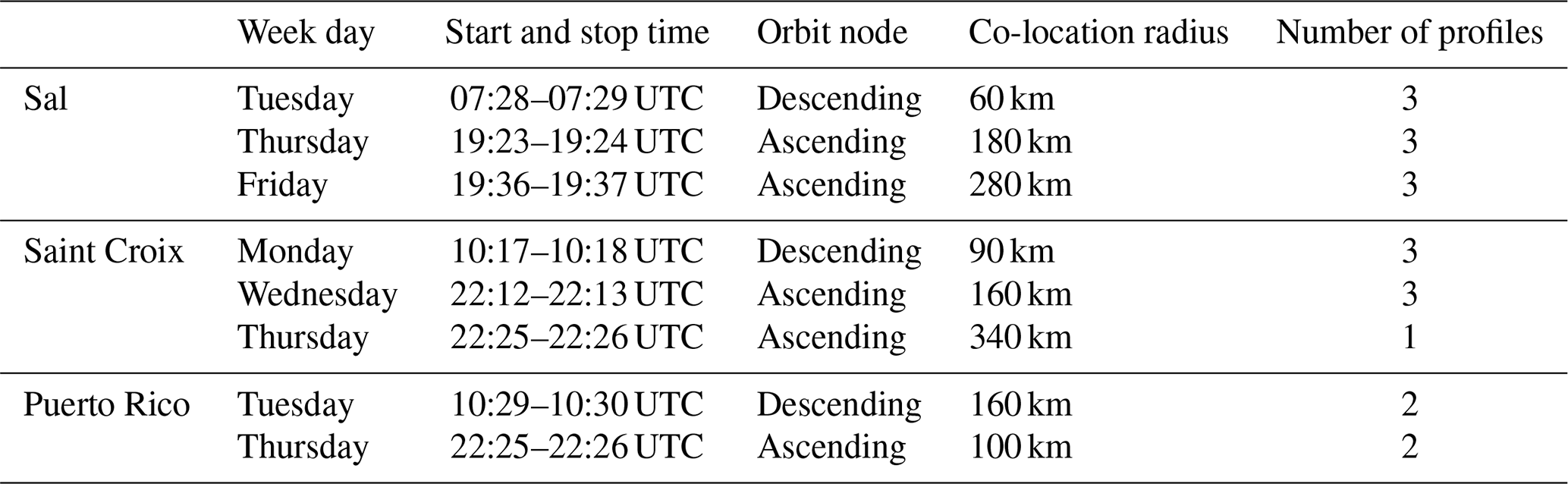
The total number of radiosonde profiles corresponding to Aeolus overpasses thus amounts to 20, of which 12 correspond to ascending and eight to descending orbits of Aeolus. An overview of the launches from the different sites can be found in Table 1, along with other co-location parameters fully discussed in Sect. 3.1.

Table 1 Overview of Aeolus overflights and associated radiosonde profiles.

2.3 EUMETSAT SAFNWC cloud type product

The Satellite Application Facility for supporting NoWCasting and very short range forecasting (SAFNWC; Alonso Lasheras et al., 2005) developed a number of satellite-based meteorological products distributed by the European Organisation for the Exploitation of Meteorological Satellites (EUMETSAT). Among others, they provide the Cloud Type (CT) product (Derrien and Le Gléau, 2005), which is a detailed scenery classification of clouds based on different main classes.

The baseline data originate from the Spinning Enhanced Visible and Infrared Imager (SEVIRI) operated onboard the second-generation METEOSAT geostationary satellites (MSG). Multispectral thresholding techniques (Saunders and Kriebel, 1988; Derrien et al., 1993; Stowe et al., 1999) are subsequently applied in the NWCSAF software to process the SEVIRI/MSG images into the various NWC products. The product is available with a temporal resolution of 15 min and a nadir spatial resolution of 3 km, compared to 11 km at the edge of the field of view.

In this study, CT is used to identify the cloud type and cloud cover along the Aeolus tracks and to assess the quality of the Aeolus wind products relative to the presence of clouds. More specifically, we identify the pixels closest to each track of Aeolus and determine the average percentage of cloud cover at each altitude based on a cloud classification. According to this classification, an observation bin is considered as cloudy if it is situated within or below a cloud. This refers to the following classes for altitudes above 16 km (very high clouds), between 7 and 16 km (high clouds), between 3 and 7 km (mid-level, low, and fractional cloud types) and finally below 3 km (very low cloud types).

2.4 CAMS dust products

The fourth generation of ECMWF Global Atmospheric Composition Reanalysis (EAC4) (Inness et al., 2019) is produced by the Copernicus Atmosphere Monitoring Service (CAMS) with the main objective of global aerosol monitoring. EAC4 relies on the ECMWF IFS, which has been extended to predict and assimilate aerosols (Rémy et al., 2019), trace gases (Flemming et al., 2015; Huijnen et al., 2019), and greenhouse gases. The IFS meteorological and atmospheric composition models are combined with data assimilation from satellite products using the 4D-EnVar data assimilation scheme in CY42R1. In particular, CAMS assimilates the aerosol optical depth (AOD) at 550 nm derived from MODIS and the Polar Multi-Sensor Aerosol Optical Properties (PMAp). Reanalysis outputs are provided on three-dimensional time-consistent fields interpolated on 25 pressure levels, a horizontal resolution of about 80 km, and a time resolution of 6 h.

Similar to the SAFNWC CT, the dust–aerosol mixing ratio is used to assess the quality of the Aeolus wind products in the presence of dust. The dust–aerosol mixing ratio is thereby averaged along each track and projected onto Rayleigh-clear and Mie-cloudy observation bins to obtain an estimate of the dust concentration for each observation.

3 Methods

3.1 Co-location criteria

For the comparison of Aeolus against radiosonde profiles, several steps are required to fit the radiosonde wind measurements to the Aeolus observation grid and to co-locate them in time and space.

To ensure vertical consistency, the high-resolution radiosonde measurements are vertically averaged within the 24 range bins as specified in the Aeolus L2B product. Subsequently, the radiosonde total horizontal wind speed V_RS and direction ϕ_RS are projected to the Aeolus HLOS (HLOS_RS) using the azimuth angle ϕ_AEOLUS also specified in the L2B product, in accordance with

$$\begin{array}{}\text{(1)}& {\text{HLOS}}_{\mathrm{RS}}=V_{\mathrm{RS}}\times \cos \left({\mathit{\varphi }}_{\mathrm{AEOLUS}}-{\mathit{\varphi }}_{\mathrm{RS}}\right).\end{array}$$

Moreover, we have chosen co-location radii of up to 340 km, as we assume typical variations in zonal wind to be of a larger scale. In fact, during boreal summer, African Easterly Waves (AEWs) and tropical disturbances dominate the tropospheric zonal wind variability over the tropical Atlantic, which generally have a horizontal wavelength of 2000–5000 km with a periodicity of 2–7 d (Belanger et al., 2016). Section 4.3.2 discusses the error dependencies related to co-location aspects in more detail.

3.2 Statistical metrics

Different metrics were used to validate and estimate the systematic and random error of Aeolus wind products. The wind speed difference between Aeolus and radiosonde along the HLOS is defined as

$$\begin{array}{}\text{(2)}& {\mathrm{\Delta }}_{{\mathrm{diff}}_{\mathrm{HLOS}}}=\left({\text{HLOS}}_{\mathrm{AEOLUS}}-{\text{HLOS}}_{\mathrm{RS}}\right).\end{array}$$

Thus, the bias μ is defined as the total mean difference

$$\begin{array}{}\text{(3)}& \mathit{\mu }={\displaystyle \frac{\mathrm{1}}{N}}\sum _{i=\mathrm{1}}^N{\mathrm{\Delta }}_{{\mathrm{diff}}_{\mathrm{HLOS}},}\end{array}$$

with the mean absolute difference (MADI) yielding

$$\begin{array}{}\text{(4)}& \text{MADI}={\displaystyle \frac{\mathrm{1}}{N}}\sum _{i=\mathrm{1}}^N\left|{\mathrm{\Delta }}_{{\mathrm{diff}}_{\mathrm{HLOS}}}\right|,\end{array}$$

and N the total number of data points.

Additionally, we calculated the standard deviation of the difference

$$\begin{array}{}\text{(5)}& \text{SD}=\sqrt{{\displaystyle \frac{\mathrm{1}}{i-\mathrm{1}}}\sum _{i=\mathrm{1}}^N{\left({\text{HLOS}}_{\mathrm{AEOLUS},i}-{\text{HLOS}}_{\mathrm{RS},i}\right)}^{\mathrm{2}}},\end{array}$$

and the scaled median absolute deviation (SMAD)

$$\begin{array}{}\text{(6)}& \begin{array}{rl}& \text{SMAD}\\ & =\mathrm{1.4826}\times \text{median}\left(|{\mathrm{\Delta }}_{{\mathrm{diff}}_{\mathrm{HLOS}}}-\text{median}\left({\mathrm{\Delta }}_{{\mathrm{diff}}_{\mathrm{HLOS}}}\right)|\right).\end{array}\end{array}$$

The SMAD is equivalent to the standard deviation for a normal distribution of errors, but is often used in Aeolus validation studies as it is less sensitive to individual outliers with very large differences than the standard deviation.

Since the number of data points varies greatly depending on the observation channel and height, we define the standard error of the mean bias ϵ_μ as

$$\begin{array}{}\text{(7)}& {\mathit{ϵ}}_{\mathit{\mu }}={\displaystyle \frac{\text{SMAD}}{\sqrt{N}}}.\end{array}$$

3.3 Representativeness

The difference between Aeolus and radiosonde observations is the sum of the Aeolus observation error, the radiosonde observation error, and the error arising from spatial and temporal displacement of the observations and different observation geometries. The latter is usually referred to as “representativeness error” (Weissmann et al., 2005). As the three error components can be assumed to be uncorrelated, the standard deviation of the Aeolus HLOS winds observation error (σ_Aeolus) can therefore be calculated as

$$\begin{array}{}\text{(8)}& {\mathit{\sigma }}_{\mathrm{Aeolus}}=\sqrt{{\mathit{\sigma }}_{\mathrm{tot}}^{\mathrm{2}}-{\mathit{\sigma }}_{\mathrm{RS}}^{\mathrm{2}}-{\mathit{\sigma }}_{\mathrm{rep}}^{\mathrm{2}}},\end{array}$$

where σ_tot is the standard deviation of the total difference between Aeolus and radiosonde observations (SD), σ_RS is the standard deviation of the radiosonde observation error, and σ_rep is the standard deviation of the representativeness error. Martin et al. (2021) estimated that the representativeness error for the comparison of Aeolus and radiosonde observations in mid-latitudes is about 2.5 m s⁻¹ based on high-resolution model simulations. As the wind fields in the area of the present validation study are comparably homogeneous, we estimate the representativeness error for our comparison to be in the range of 1.5–2.5 m s⁻¹. Note that, despite the integration lengths differing, we average Rayleigh and Mie observations over the same co-location area, which allows for the application of a consistent representativeness error range for both channels. The radiosonde observation error σ_RS is estimated to be 0.7 m s⁻¹ based on Dirksen et al. (2014).

The representativeness and radiosonde observation errors also need to be considered when comparing the differences between Aeolus and radiosonde observations with the expected error provided in the Aeolus data product (EE_Aeolus). To account for this, we add the radiosonde observation error and an estimated representativeness error of 2 m s⁻¹ to achieve the total expected error for the comparison (EE_tot) as follows:

$$\begin{array}{}\text{(9)}& {\text{EE}}_{\mathrm{tot}}=\sqrt{{\text{EE}}_{\mathrm{Aeolus}}^{\mathrm{2}}+{\mathit{\sigma }}_{\mathrm{RS}}^{\mathrm{2}}+{\mathit{\sigma }}_{\mathrm{rep}}^{\mathrm{2}}}.\end{array}$$

3.4 Quality control

Quality control (QC) is an important step in the evaluation of Aeolus wind errors. The aim is to check for the validity of the observations and discard nonphysical wind results from the analysis process. The QC we apply here is based on the existing QC recommendations (Rennie and Isaksen, 2020) from the Aeolus Data Science and Innovation Cluster (DISC), and primarily rely on the HLOS wind error estimate (EE_Aeolus) in the L2B product and the validity flags.

The Rayleigh channel EE_Aeolus is based on the uncertainty of the SNR spectrometer response and takes into account error propagation arising from the sensitivity of the Fabry–Pérot interferometer, Poisson noise in the useful signal, and the solar background. Ultimately, the Rayleigh EE_Aeolus is proportional to the inverse square root of the useful signal on the detector. Future baseline versions are foreseen to also include contributions to the EE caused by uncertainties of NWP temperature and pressure used in the processor for instrument calibration procedures as well as the one caused by an insufficient correction of the narrowband particulate return that is transmitted to the Rayleigh channel (Dabas et al., 2008). By contrast, the Mie EE_Aeolus is determined from the accuracy of the fringe peak position using the solution covariance of the Lorentzian fitting algorithm based on four characteristics of the signal shape, i.e. the peak position, height, width, and offset.

Following the default QC flags, all Aeolus wind products with a validity flag of 0, EE_Aeolus over 8 m s⁻¹ for Rayleigh and 4 m s⁻¹ for Mie, are omitted. Nevertheless, the QC used might not be enough and the data algorithm may contain gross errors in the wind estimate that have not been flagged as invalid. These errors are usually due to non-Gaussian error sources, such as instrument/transmission failure, or to a misrepresentation of the observations in space and time. Since the two aforementioned QC are not sufficient to remove these gross errors, an additional QC parameter is used, namely the modified Z score (Lux et al., 2022b; Witschas et al., 2022; Iglewicz and Hoaglin, 1993). The modified Z score Z_m,i is defined as

$$\begin{array}{}\text{(10)}& Z_{m,i}={\displaystyle \frac{{\mathrm{\Delta }}_{{\mathrm{diff}}_{\mathrm{HLOS}}}-\text{median}\left({\mathrm{\Delta }}_{{\mathrm{diff}}_{\mathrm{HLOS}}}\right)}{\text{SMAD}}},\end{array}$$

and describes the median deviations between each wind speed difference normalised with the SMAD. The modified Z score significantly influences small data sets, such as those used in this study. Following literature recommendations (Lux et al., 2022b; Witschas et al., 2022; Sandbhor and Chaphalkar, 2019; Tripathy et al., 2013), we discard wind observations with a modified Z score greater than 3 as a final QC.

4 Results

4.1 Statistical comparison of Aeolus with radiosonde observations and model winds

In this section, the L2B HLOS winds (L2bP 3.50) from Aeolus are compared statistically with radiosonde observations and model winds. This includes a comparison with the ECMWF model equivalents (Sect. 4.1.1), an overview of systematic and random differences with respect to Cal/Val sites and orbital nodes (Sect. 4.1.2), and finally the identification of an orbital- and altitude-dependent bias in the Rayleigh-clear channel (Sect. 4.1.3).

The present study relies on a total of 384 Rayleigh-clear and 59 Mie-cloudy bin pairs, of which ∼ 60 % and ∼ 53 % are from ascending orbits, respectively, with the majority of observations obtained from the Caribbean launch sites (∼ 56 % for Rayleigh-clear and ∼ 64 % for Mie-cloudy). Rayleigh-cloudy bin pairs are also available, but only in a very small number (16 counts), which makes statistical analysis difficult.

4.1.1 Comparative analysis with radiosondes and ECMWF model equivalents

Figure 1 shows a scatter plot of the radiosonde HLOS (HLOS_RS) against Aeolus L2B (HLOS_AEOLUS) wind products (a) as well as against Aeolus ECMWF model equivalents (HLOS_ECMWF) (b). The × symbol represents the gross errors rejected with a Z-score threshold of 3 (∼ 3.5 %, ∼ 4.8 %, and ∼ 6.7 % of the total Rayleigh-clear, Mie-cloudy, and Rayleigh-cloudy data points, respectively). The Aeolus model equivalent HLOS_ECMWF for Rayleigh-clear shows a much better agreement with the radiosonde observations HLOS_RS, with an SD of 2.1 m s⁻¹ (Fig. 1b) compared to the Aeolus HLOS_AEOLUS Rayleigh-clear observations, which have a larger spread and an SD of 4.8 m s⁻¹ (Fig. 1a). The systematic difference of the model equivalent is also smaller with a bias of 0.1±0.1 m s⁻¹ compared to $-\mathrm{0.5}\pm \mathrm{0.2}$ m s⁻¹ for the Aeolus observations. By contrast, the Mie-cloudy winds of both Aeolus model equivalents and HLOS_AEOLUS behave similarly with respect to the radiosonde observations, with SDs of 2.93 and 2.9 m s⁻¹, respectively. Again, the systematic difference in the model equivalent is smaller than for Aeolus Mie-cloudy winds, with biases of 0.4±0.3 and $-\mathrm{0.9}\pm \mathrm{0.3}$ m s⁻¹, respectively. For Rayleigh-cloudy, the SD is larger at 6.6 m s⁻¹ with a bias of 1.0±1.4 m s⁻¹, but given the small statistical sample size, there is a risk of a large margin of error. The generally good agreement between radiosonde and model equivalent shows that the co-location parameters used in this study are reliable, as most of the random errors seem to be specific to the Aeolus Rayleigh-clear data. This stresses the need to identify the underlying potential error sources of Rayleigh-clear observations with respect to the presence of clouds and dust aerosols, which are frequent in the region of interest. It is also worth noting that this good agreement indicates that the model equivalent is a robust reference for validating the Aeolus winds in the tropical Atlantic.

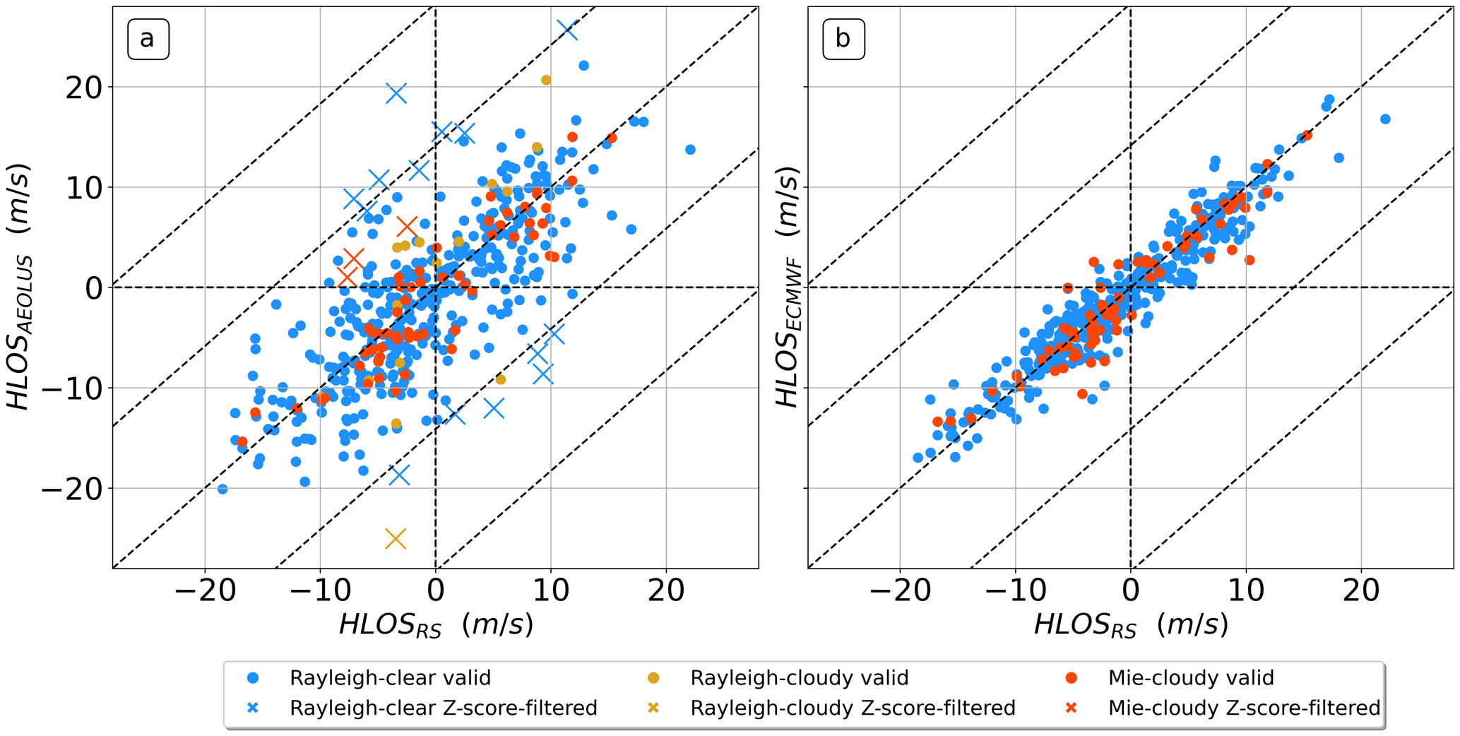
Figure 1 (a) Aeolus HLOS Rayleigh-clear (blue), Mie-cloudy (red), and Rayleigh-cloudy (gold) wind products plotted against radiosonde observations projected along the HLOS for the 20 radiosonde profiles. The gross errors (crosses) are determined using the modified Z score with a threshold of 3. (b) Aeolus HLOS model equivalents from the ECMWF model background plotted against radiosonde observations. The dashed lines are located at the ±10 and ±20 m s⁻¹ wind speed difference between two observations.

4.1.2 Systematic and random errors using radiosondes

An overview of the bias and random differences of both channels can be found in Table 2. In terms of systematic errors, Rayleigh-clear shows a relatively small negative bias of $-\mathrm{0.5}\pm \mathrm{0.2}$ m s⁻¹, on average, which is below the ESA specification of 0.7 m s⁻¹ (Ingmann and Straume, 2016). This bias is, however, the result of a large heterogeneity with respect to the Cal/Val sites and orbital nodes, with compensating biases of $-\mathrm{1.5}\pm \mathrm{0.6}$ and 0.6±0.4 m s⁻¹ for the descending and ascending nodes on Sal, respectively, compared to negative biases of $-\mathrm{1.0}\pm \mathrm{0.3}$ m s⁻¹ (ascending) and $-\mathrm{0.6}\pm \mathrm{0.4}$ m s⁻¹ (descending) in the Virgin Islands. As for random differences, Rayleigh-clear has an average SD of 4.8 m s⁻¹, which varies only marginally between the Cal/Val sites and orbital nodes, ranging from 4.1 to 5.3 m s⁻¹. The overall SMAD is found to be slightly below at 4.3 m s⁻¹.

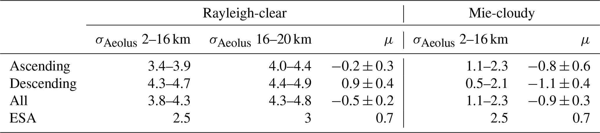
For comparison with the ESA recommendation for random errors, we derived the random errors for Aeolus observations considering also the representativeness errors for the comparison and radiosonde observation errors according to Eq. (8) (Table 3). The random error at 2–16 km altitude of 3.8–4.3 m s⁻¹ exceeds the threshold of 2.5 m s⁻¹, while at 16–20 km altitude it amounts to 4.3–4.8 m s⁻¹, also exceeding the ESA threshold of 3 m s⁻¹. The quality of Rayleigh-clear observations primarily depends on the signal accumulation, which can vary with the thickness of the RBS and the horizontal accumulation length as well as with the atmospheric path signal. The latter has been decreasing in recent years as a result of initial instrumental misalignment, laser-induced contamination, as well as the wavefront error of the 1.5 m telescope. The solar background noise, which varies along the orbit and season, can also affect the quality of the Rayleigh-clear observations.

Table 2 Overview of the mean bias and standard error of the mean bias (μ, ϵ_μ; m s⁻¹), standard deviation (SD; m s⁻¹), scaled median absolute deviation (SMAD; m s⁻¹), and counts (COUNT) for the Rayleigh-clear and Mie-cloudy channels, orbital nodes, and the different radiosonde locations for all altitude ranges. Due to the small number of available data, Rayleigh-cloudy is not shown here.

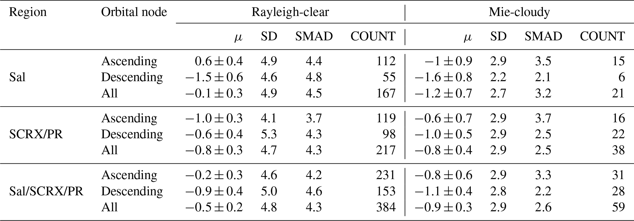
For Mie-cloudy, the systematic difference reveals a bias of $-\mathrm{0.9}\pm \mathrm{0.3}$  m s⁻¹, falling within the ESA specified uncertainty range when considering the standard error of the bias. This bias remains relatively consistent across regions and orbital nodes, with a slightly larger bias observed in the descending orbits and over Sal. Concerning the random differences, the observations exhibit a total random error of 1.1–2.3 m s⁻¹, which is below the ESA 2–16 km recommendation, as most Mie-cloudy observations are located underneath 16 km altitude. As with the bias, the SD and SMAD of Mie-cloudy are also quite independent of orbital and regional dependence. The overall accuracy of Mie-cloudy depends on the signal accumulation, the classification algorithm, and the quality of the calibration data. The accuracy of Mie-cloudy winds is higher than that of Rayleigh-clear winds as particle backscatter is usually stronger than that of clear air, in addition to the fact that Mie backscatter is not subject to broadening induced by Rayleigh–Brillouin scattering (Witschas et al., 2012).

Table 3 Overview of the random (σ_Aeolus; m s⁻¹) errors at altitude ranges 2–16 and 16–20 km as well as systematic (μ, ϵ_μ; m s⁻¹) errors derived according to Eq. (8) for Rayleigh-clear and Mie-cloudy winds. The errors are presented for the different orbital nodes, alongside ESA error recommendations. The random error σ_Aeolus was computed for a representativeness error σ_rep ranging from 1.5 to 2.5 m s⁻¹. For Mie-cloudy, only the altitude range 2–16 km is shown for the random error, as Mie-cloudy does not sample sufficiently above 16 km.

Comparing the results of different Cal/Val studies is tricky as the influence of geographical regions, atmospheric conditions, decreasing laser energy, and product baseline and quality control procedures on the result can be significant and must be considered.

In this analysis, comparisons are only made with statistics derived from airborne wind lidar measurements acquired during the AVATAR-T campaign, which was also part of JATAC (Witschas et al., 2022; Lux et al., 2022b). In particular, the statistics derived from a heterodyne detection wind lidar (2 µm DWL) flown onboard the DLR Falcon research aircraft are used for comparison. Due to the high sensitivity of the heterodyne detection principle, the 2 µm DWL provides accurate wind speed data even in a clear atmosphere where Aeolus only provides Rayleigh-clear winds. Hence it is a well-suited reference instrument for the validation of both Rayleigh-clear and Mie-cloudy winds. The statistical analysis of AVATAR-T shows systematic errors of $-\mathrm{0.1}\pm \mathrm{0.3}$ m s⁻¹ for Rayleigh-clear and $-\mathrm{0.7}\pm \mathrm{0.2}$ m s⁻¹ for Mie-cloudy, which are slightly smaller than for radiosondes. However, the random error of 7.1±0.3 m s⁻¹ for Rayleigh-clear is significantly higher. The difference in results is caused by the different altitudes at which the data are sampled, as the aircraft only samples the lower 10 km portion of the troposphere, which is shown to be more noisy owing to the abundance of dust aerosols in this region. For Mie-cloudy, the random error gives 2.9±0.3 m s⁻¹, which is similar to our radiosonde-based results, as most Mie-cloudy scattering occurs at lower levels.

4.1.3 Orbital bias in the Rayleigh-clear channel

Figure 2 shows vertical profiles of the differences between Aeolus Rayleigh-clear and radiosonde observations projected along HLOS (O-RS; solid lines), and the corresponding ECMWF model equivalents (O-B; dotted lines) for both ascending (red) and descending (blue) orbits over Sal (a), Puerto Rico, and Saint Croix (b). The shading represents the standard error of the mean bias ϵ_μ. To better understand the variations in wind speed between the orbits and enable easy comparisons with other studies (e.g. Borne et al., 2023), which also documented this bias within the model coordinate system, we have adopted the model sign convention. This involves multiplying the HLOS wind descending tracks by −1. The vertical profiles illustrate the presence of an ascending/descending bias visible in both the O-B and O-RS profiles, reaching 2.5 m s⁻¹ around 8 km altitude in both regions. The differences below 5 km altitude could be related to the greater amount of dust in Cabo Verde during this period, while above 17 km the differences could partly be related to the lack of descending orbit data over Sal (Fig. 2a). This altitude- and orbit-dependent bias was already described by Borne et al. (2023) using first-guess departure statistics over West Africa.

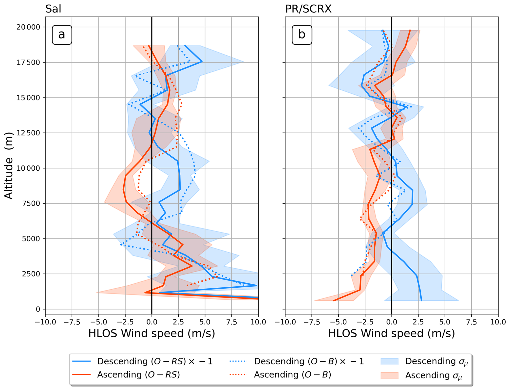
Figure 2 Average differences between Aeolus (O) and radiosonde (RS) wind observations (solid lines) and standard error for (a) Sal and (b) Puerto Rico/Saint Croix for descending (blue) and ascending (red) profiles. Average differences with ECMWF model equivalents (B) are given as dotted lines. The lines were smoothed vertically using a three-value moving average. To comply with the sign convention of the model coordinate system, the HLOS winds from the descending orbit are multiplied by −1.

This latitude consistent bias caused the zonal winds in the ECMWF analysis to accelerate in the morning and weaken in the evening, affecting the African Easterly Jet (AEJ) and Tropical Easterly Jet (TEJ) in particular. Correcting this bias with a temperature-dependent approach helped to improve the representation of winds in the analysis and forecast fields (Borne et al., 2023). However, the cause of this bias remains unknown, as it has not been proven to be related to temperature, nor has any dependence on wind speed, SNR, or useful signal been found (not shown here). Here, as both the O-B and O-RS profiles are very close to each other, with deviations below 0.5 m s⁻¹, the existence of this bias can be confirmed observationally with radiosondes. As highlighted by Horányi et al. (2015), biases of the order of 1 m s⁻¹ can already deteriorate forecast quality.

4.2 Error dependency

In this section we examine the error dependency and associated error sources of the different Aeolus wind products. Firstly, we investigate the error dependency as a function of co-location parameters, such as radius and time difference between two observation points, to account for representativeness. Secondly, we explore the error dependency in relation to the presence of clouds and dust, as these presumably influence the quality of Aeolus wind products.

4.2.1 Temporal and spatial co-location

Rayleigh-clear and Rayleigh-cloudy

Figure 3 shows the absolute difference between Aeolus and radiosonde observation points $\left|{\mathrm{\Delta }}_{{\mathrm{diff}}_{\mathrm{HLOS}}}\right|$ as a function of EE_tot (a), altitude (b), co-location radius (c), and co-location time (d) for the Rayleigh-clear (blue) and Rayleigh-cloudy (gold) observation types. The solid and dashed blue lines show the Rayleigh-clear MADI and SMAD, respectively, with each value calculated using a minimum sample size of 40 data points for panels (a), (b), and (d). Also shown are outliers (cross symbol +), which we define in this study as values with low EE_Aeolus (< 5 m s⁻¹) and large absolute difference (> 10 m s⁻¹), which are of particular interest as they contribute the most to the wind quality degradation. The Rayleigh-clear outliers account for 13 observations, i.e. ∼ 3.4 % of the data points. For Rayleigh-cloudy, no MADI and SMAD are computed due to the lack of data.

In general, the MADI and SMAD between Rayleigh-clear and radiosonde wind observations appear to be proportional to the Aeolus EE_tot (Fig. 3a), with larger deviations associated with larger EE_tots, as expected. For Rayleigh-cloudy observations, it is difficult to establish a dependency although the absolute difference appears to be generally greater owing to the large SD of 6.6 m s⁻¹ for this observation type. Considering the altitude error dependency of Rayleigh-clear (Fig. 3b), a general pattern emerges with MADI and SMAD reaching a minimum of 3 and 2 m s⁻¹, respectively, on average in the middle troposphere at 10 km, while increasing above and below, with MADIs of 4–5 m s⁻¹ and SMADs of almost 6 m s⁻¹ at 2.5 and 19 km altitude. As we will see in Sect. 4.2.2, this error pattern is inversely proportional to the Rayleigh backscattered useful signal, as it directly affects the SNR and thereby the quality of the observation points. Rayleigh-clear outliers seem to occur at all altitudes and Rayleigh-cloudy observations are primarily found in the lower troposphere, below 6 km.

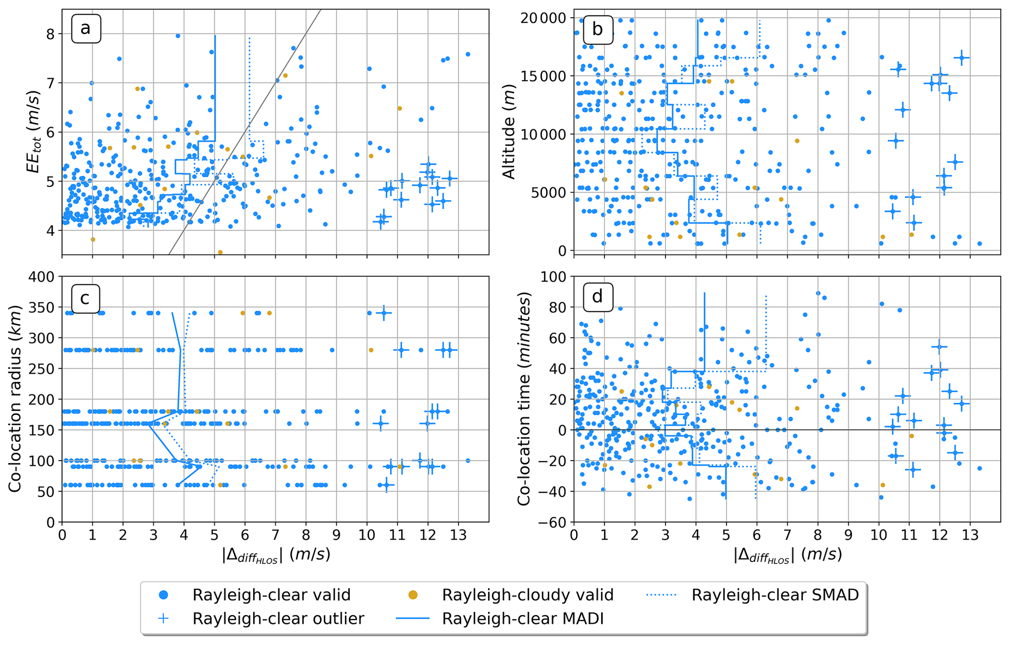
Figure 3 EE_tot (a), altitude (b), co-location radius (c), and co-location time (d) quantities expressed as a function of the absolute difference between radiosonde HLOS winds (HLOS_RS) and Aeolus (HLOS_AEOLUS) Rayleigh-clear (blue) and Rayleigh-cloudy (gold) observations. Outliers are defined as values with an EE_Aeolus below 5 m s⁻¹ and absolute difference larger than 10 m s⁻¹ and are represented by the cross symbol +. The solid stepwise blue lines indicate the MADI, and the dotted blue lines represent the SMAD of Rayleigh-clear. Each step encompasses a minimum of 40 data points to ensure significance. The grey line in panel a represents the diagonal at intercept 0 with slope 1. Due to the limited number of data, no MADI and SMAD are shown for Rayleigh-cloudy.

In Fig. 3c we examine the error dependency with respect to the co-location radius, which extends up to 340 km, a distance that is large relative to the 100 km specified in the ESA recommendations. However, the MADI and SMAD for Rayleigh-clear do not increase with the radius, but stagnate at an average of 3–4 m s⁻¹ for radii above 100 km, while they are slightly higher below 100 km, reaching 4–5 m s⁻¹. Furthermore, outliers appear across all co-location radii. This indicates that the use of a co-location distance up to 340 km is acceptable for the statistical comparison. Exploring the error dependency with respect to the time difference between the observations (Fig. 3d), there is an indication for increasing differences for larger time differences, going from 3–4 m s⁻¹ at 0 min to 4–6 m s⁻¹ above 30 min. There is also an asymmetry of the error dependence, with a larger error magnitude for radiosonde observations preceding the Aeolus passage. Since most radiosondes were launched with the objective of reaching the mid-troposphere during the satellite's passage, the observations preceding (following) Aeolus of more than 30 min correspond mainly to observations at lower (higher) altitudes. The larger MADI and SMAD values for these time differences could hence be an indirect effect of the larger errors found at those altitudes (Fig. 3b). Again, no error dependency is observed for outliers, with most occurring below ±40 min time differences.

Mie-cloudy

Figure 4 shows the same error dependencies as in Fig. 3, but for the Mie-cloudy observation type. For Mie-cloudy, we define outliers as values exceeding an absolute error of 6 m s⁻¹ along with EEs inferior to 3 m s⁻¹. With a total of three data points, they account for ∼ 5 % of the total Mie-cloudy observations. In panels (a), (b), and (d), each MADI and SMAD value is calculated using a minimum sample size of 15 data points.

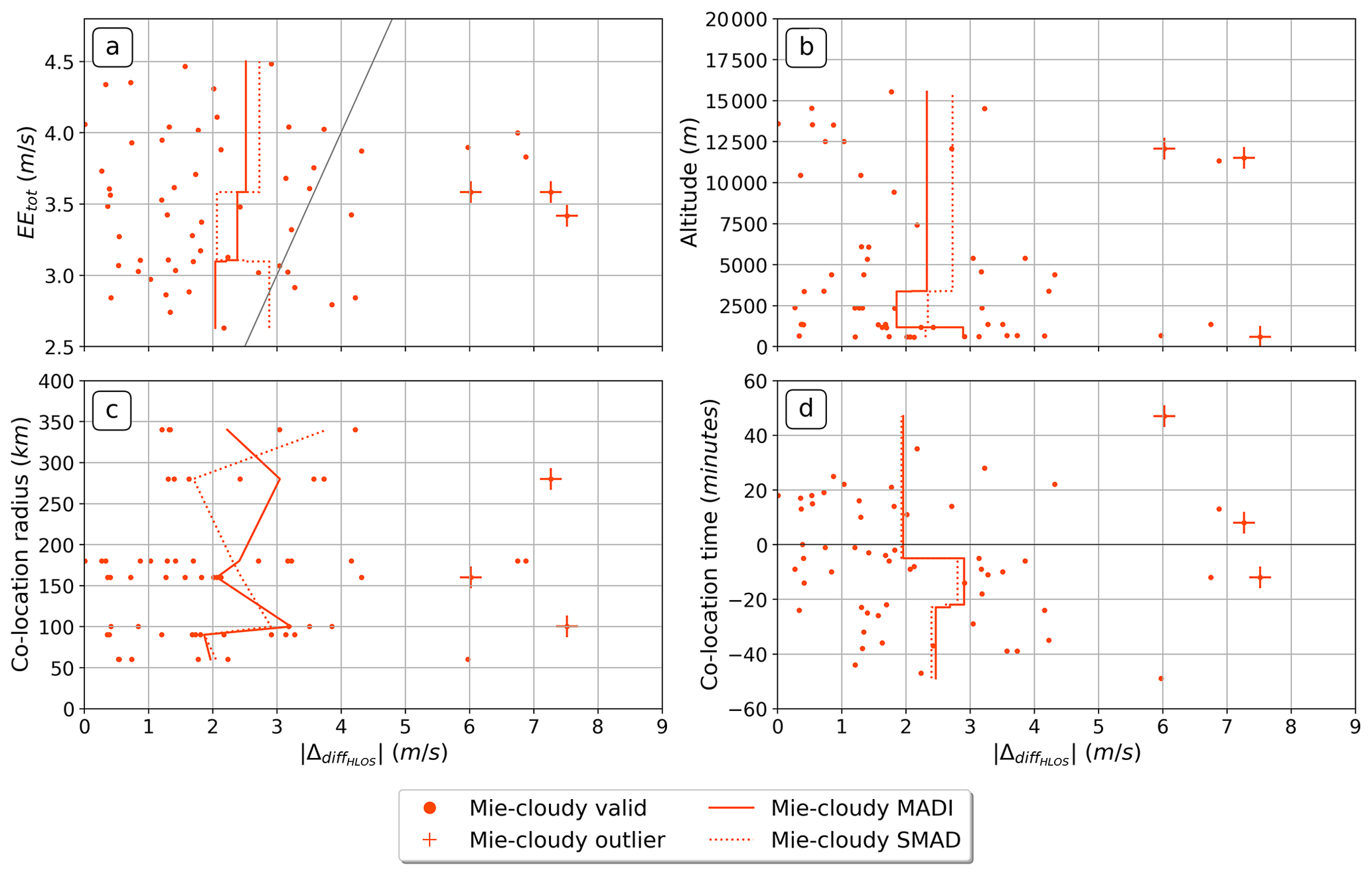
Figure 4 Same as for Fig. 3, but for Mie-cloudy. For Mie-cloudy (red), outliers are defined as values having an absolute error above 6 m s⁻¹ and an EE_Aeolus inferior to 3 m s⁻¹. The MADI and the SMAD values are computed using a minimum sample size of 15 data points.

As shown in Fig. 4a, the absolute differences for Mie-cloudy observations are generally smaller than for Rayleigh-clear, with the largest deviations being around 7–8 m s⁻¹, while attaining 13–14 m s⁻¹ for Rayleigh-clear. The SMAD remains between 2 and 3 m s⁻¹, indicating an overestimation of the EE_tot, especially for increasing EE_tot. Regarding the altitude error dependency (Fig. 4b), most of the data are found within the 10–15 km layer, which is probably related to the presence of high-level clouds, and below 7 km, where low- and mid-level clouds and dust layers are found. Due to the sparseness of Mie-cloudy data, both MADI and SMAD do not show a specific vertical error trend. While MADI and SMAD remain between 2.3 and 2.7 m s⁻¹, respectively, they decrease to 1.8 and 2.3 between 1.5 and 3 km altitude before increasing to almost 3 m s⁻¹ in the lowest 1 km. Figure 4c shows that similarly to Rayleigh-clear, Mie-cloudy reveals no error dependency with respect to co-location radii, with the mean absolute error and SMAD mainly ranging from 1.7 to 3.2 m s⁻¹, and outliers found at all radii. Regarding the error dependence on time difference (Fig. 4d), we find that most of the observation differences occur at time intervals of less than ±40 min. MADIs and SMADs are generally higher for negative co-location times, corresponding to cases where radiosonde observations are sampled before those from Aeolus. Nevertheless, we do not notice a strong relationship between co-location time and errors.

4.2.2 Cloud type and dust

As already mentioned, the accuracy of Rayleigh-clear and, to a lesser extent, Mie-cloudy depends on the signal level and SNR. In general, the signal level depends on the range bin thickness, the horizontal accumulation length, the atmospheric path signal, and the overall signal background level. In addition, Rayleigh-clear winds are sensitive to signal attenuation due to atmospheric conditions, with weaker signal return under optically thick clouds and dust-aerosol layers. Mie-cloudy is less affected as backscatter from particles is stronger, although it is sensitive to weak backscatter, e.g. from dust layers. Because of its strong sensitivity to signal levels, the EE_Aeolus of Rayleigh-clear only considers Poisson noise and is therefore inversely proportional to the square root of the useful signal. For Mie-cloudy, this rule of thumb is not true. In this context, we aim to investigate the quality of the Rayleigh-clear and Mie-cloudy winds and the reliability of the corresponding EE_Aeolus with respect to the presence of clouds and dust.

Rayleigh-clear

Table 4 describes the error dependency of the Rayleigh-clear observations with respect to the presence of clouds and dust, with cases below 50 %, above 50 %, and above 75 % of cloudiness, as well as sub-categories distinguishing the dust mixing ratio above (Dust) and below (Dust_NO) 10⁻⁸ kg kg⁻¹. Note that SMAD is not used for this analysis as this reliably removes outliers, which ought to be quantified here. We note that the MADI, the SD, and the EE_tot all increase with the amount of clouds and dust along the track, presumably due to the reduced return signal. In non-dusty conditions (Dust_NO), we observe that for low cloud cover (< 50 %), the SD (4.3 m s⁻¹) is lower than the EE_tot (4.8 m s⁻¹) with a difference of 0.5 m s⁻¹, while for higher cloud cover, the SD is higher compared to the EE_tot (with the difference reaching 0.1 and 0.3 m s⁻¹ for over 50 % and 75 % of cloudiness, respectively). This phenomenon is further enhanced at higher dust concentrations, with the SD reaching even higher values (6.4 m s⁻¹) than the EE_tot (5.8 m s⁻¹) for cloud cover over 75 %. This highlights how the EE_tot in clear sky conditions is well calibrated, while it becomes gradually too low with the increasing presence of clouds and dust. The larger SD with increasing cloudiness and dust concentration suggests an increasingly perturbed pattern of Rayleigh-clear observations, possibly owing to the lower signal levels or to a cross-talk.

Table 4 Overview of the total error estimate (EE_tot; m s⁻¹), mean absolute difference and standard error of the mean bias (MADI, ϵ_μ; m s⁻¹), standard deviation (SD; m s⁻¹), and counts (COUNT) for the Rayleigh-clear observations under different cloud and dust conditions. This includes three categories of cloud cover (< 50 %, > 50 %, > 75 %) and two dust mixing ratio sub-categories (>10⁸ (Dust), <10⁸ (noDust) kg kg⁻¹) along the track.

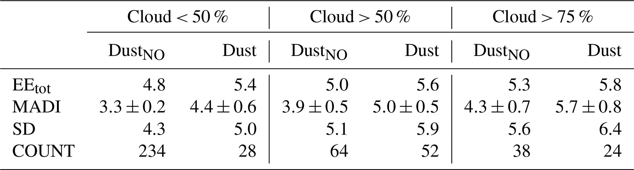
Figure 5 puts this phenomenon into perspective, by showing the altitude-dependent absolute difference $\left|{\mathrm{\Delta }}_{{\mathrm{diff}}_{\mathrm{HLOS}}}\right|$ (a, e), the EE_tot (b, f), the normalised useful signal (c, g), and the SR (d, h), where the colouring depends on the percentage of SAF clouds (upper row) and on the CAMS dust mixing ratio (lower row) along the track. For reference, the values that did not pass the QC are shown by faint symbols. In addition, Fig. 5a includes the MADI of four cloud cover percentage categories, where each MADI is computed with a minimum sample size of 10 values. The colouring in Fig. 5 is illustrative of the results summarised in Table 4, with observations showing generally greater MADI under high cloud cover (red, orange, Fig. 5a) than under lower cloud cover (blue, blue-green). Observations in the lower troposphere are naturally more strongly affected by cloud cover compared to higher levels. The same applies to dust (Fig. 5e), which also occurs mainly in the lower 5 km of the troposphere.

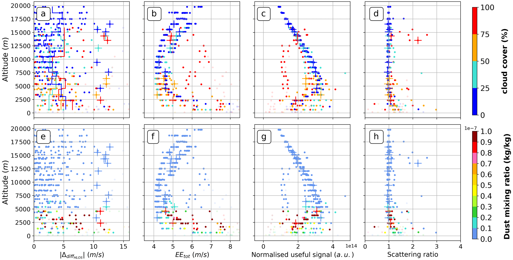
Figure 5 Altitude as a function of Rayleigh-clear absolute difference $\left|{\mathrm{\Delta }}_{{\mathrm{diff}}_{\mathrm{HLOS}}}\right|$ (a, e), EE_tot (b,f), normalised useful signal (c, g), and SR (d, h), where the colouring is dependent on the percentage of SAF clouds (upper row) and on the CAMS dust mixing ratio (lower row) along the track. The cross symbol + stands for outliers and defines values with an EE_Aeolus below 5 m s⁻¹ and an absolute difference of more than 10 m s⁻¹. The faint ^* symbols serve as references for values that did not meet the QC criteria. Panel (a) includes the MADI for each cloud cover percentage, with a minimum sample size of 10 data points used to compute each value.

As we have shown in Fig. 3b, the absolute error is higher in the upper and lower troposphere and minimised in the middle troposphere around 10 km altitude. This trend is well reflected in the EE_tot in Fig. 5b, which is an indication of the generally good consistency between the EE_tot and the absolute differences. As expected, this tendency fits inversely with the normalised useful signal shown in Fig. 5c, with lower signal in the upper and lower troposphere. Indeed, in the higher troposphere the air is less dense and the thickness of the range bins is not sufficient to compensate for the decrease in air molecule density. In the lower troposphere, the return signal is lower due to strong attenuation under clouds and dust layers. Interestingly, the values with high EE_tot and smaller useful signal in the mid-troposphere between 5 and 12.5 km in red most likely correspond to observations sampled under thick clouds, resulting in a strongly attenuated signal. They account for most of the observations with cloud cover greater than 75 % in this altitude range, while the cloud tops appear to be located between 12.5 and 15 km, as they exhibit a larger normalised useful signal and an SR greater than 1 (Fig. 5d, h). Finally, outliers are found under all types of cloud and dust conditions and affect different altitude ranges. They also occur for regular normalised useful signals, with most SRs lying around 1, which rules out a cause related to atmospheric particles.

Mie-cloudy

Table 5 shows the same results as Table 4, but for Mie-cloudy. Due to the limited number of data for Mie-cloudy winds, the interpretation of the results should be treated with caution. We find that, in contrast to Rayleigh-clear, the EE, MADI, and SD decrease with the percentage of cloud cover along the path. This is understandable as clouds provide the strongest backscatter signal required for high-quality Mie-cloudy observations. However, the presence of dust for cloud cover below 50 % leads to a decrease in EE_tot, MADI, and SD, while conversely there is an increase of these quantities in more dense cloudy conditions (> 50 %, > 75 %). A possible explanation is that in clear-sky conditions, the backscatter from dust layers is strong enough to obtain high-quality observations, whereas in cloudy conditions, the attenuation by clouds weakens the backscatter return from the dust.

Table 5 Same as Table 4, but for Mie-cloudy.

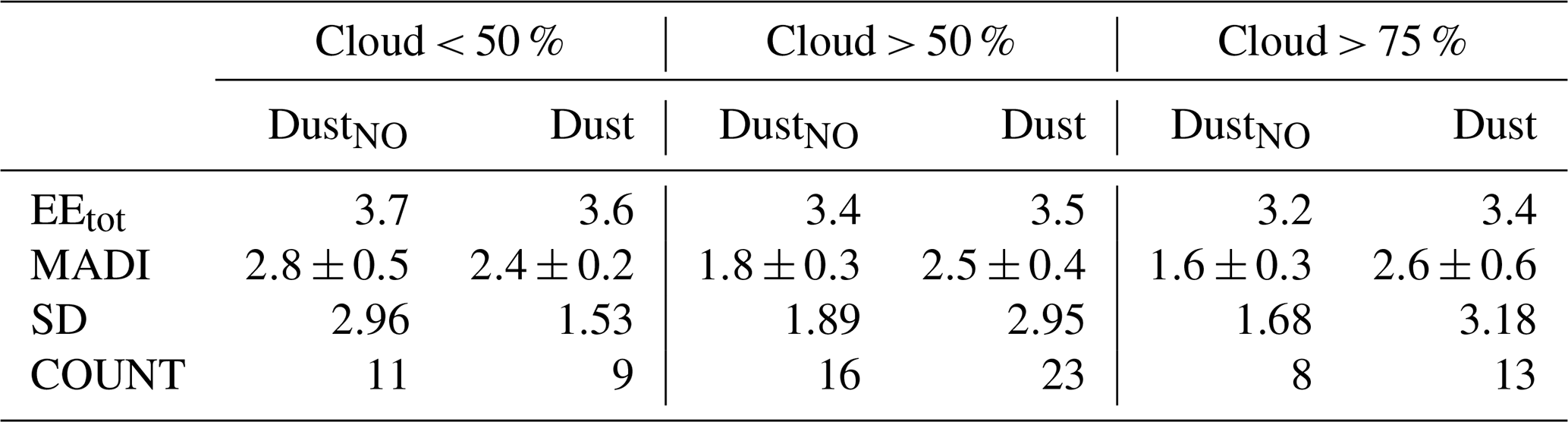
Figure 6 depicts the same results as Fig. 5, but for Mie-cloudy. As mentioned in the previous section for Fig. 4b, most backscatter occurs in two layers, i.e. within 10–15 km and below 7 km altitude. The majority of observations have normalised useful signals above 5×10¹⁵ arbitrary units (a.u.) (Fig. 6c, g), which is overall above the normalised useful signal of the rejected observations shown in transparent. Furthermore, the SRs are generally over 1 (Fig. 6d, h), which is characteristic of Mie-cloudy observations. More specifically, observations sampled above 12.5 km have a cloud cover of more than 75 % along the track and probably correspond to cloud tops, as they have stronger SRs between 1.5 and 3 (Fig. 6d, h). Between 7.5 and 12.5 km altitude, most of the observations occur with cloud cover of less than 50 %, with SRs falling below 1.3. In this altitude range, there are also two outliers, which interestingly have SRs around 1 and a normalised useful signal in the same order of magnitude as the discarded ones. Their presence is unusual, as Mie-cloudy observations are only obtainable for SRs over 1. This highlights the fact that some artefacts were not flagged correctly by the QC process. Finally, below 7.5 km, the cloud cover is mainly more than 50 %, while the dust concentration is mainly below $\mathrm{5}\times {\mathrm{10}}^{-\mathrm{8}}$ kg kg⁻¹, showing that most of the Mie-cloudy backscatter results from clouds and not from dust. As can be seen in Fig. 6g, observations with high dust concentration (brown) are discarded (transparent) with normalised useful signals below 5×10¹⁵ a.u. Two observations also show negative SRs, which is an artefact, due to insufficient background signal corrections. The third outlier in the lower 1 km does not have abnormal characteristics compared to other observations at this altitude.

Figure 6 Same as Fig. 5 but for Mie-cloudy. Here the cross symbol + defines values with an EE_Aeolus below 3 m s⁻¹ and an absolute difference over 6 m s⁻¹.

4.2.3 Case studies

To further investigate the properties of the Aeolus wind errors, this section presents three case studies comparing Aeolus and radiosonde wind observations under three different atmospheric conditions, namely clear sky, high cloud cover, and high dust concentration.

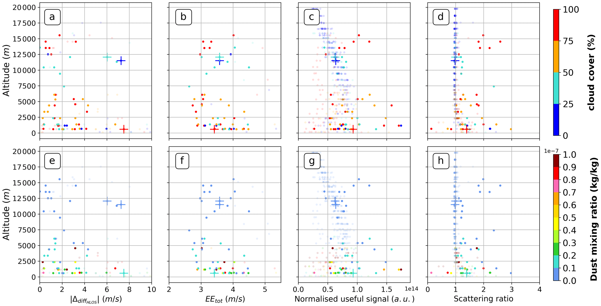
The first case study illustrated in Fig. 7 presents a comparison between Aeolus and radiosonde wind observations collected under clear-sky conditions. The radiosonde was launched over Sal Airport at 18:45 UTC on 9 September 2021, and Aeolus passed over on an ascending orbit between 19:23:56 and 19:24:31 UTC within a co-location radius of 180 km around the launch site. Figure 7a depicts the corresponding sampled radiosonde HLOS wind profile (black line) as well as Rayleigh-clear (blue) wind measurement points with associated EE_tot shown as error bars and ECMWF model equivalents shown as stepped lines. The corresponding Rayleigh-clear EE_tot, normalised useful signal and CAMS dust mixing ratio profiles are shown in blue in Fig. 7b, c and d, respectively, along with all other profiles in grey and the average of all profiles in black. Figure 7e shows the SAFNWC CT over the Cabo Verde region at 19:00 UTC. In the latter panel, it can be seen that conditions were predominantly cloud-free along the Aeolus track (solid red line) and within the co-location radius (solid white line), while some low clouds can be found in the surrounding area. In these clear-sky conditions, it is not surprising to find that most of the observations are of the Rayleigh-clear type (Fig. 7a). Throughout the atmosphere above 2.5 km, the quality of Rayleigh-clear is very good, with most error bars overlapping with radiosonde observations and ECMWF model equivalents. In general, we found that the EE_tot estimate (Fig. 7b) is below average throughout the atmosphere, with a minimum of 4.2 m s⁻¹ at 8 km altitude and a maximum above 5.5 m s⁻¹ at 17.5 and 2.5 km altitude. This is consistent with the normalised useful signal (Fig. 7c) close to the average, except between 2.5 and 12.5 km, where it is higher, most likely due to the absence of cloud attenuation. In general, EE_tot and normalised useful signal decrease below 5 km, which is accompanied by an increase in the dust mixing ratio. This increase reaches 1.2 kg kg⁻¹ at about 2 km altitude, below which no observations are found, presumably filtered out during the QC procedure.

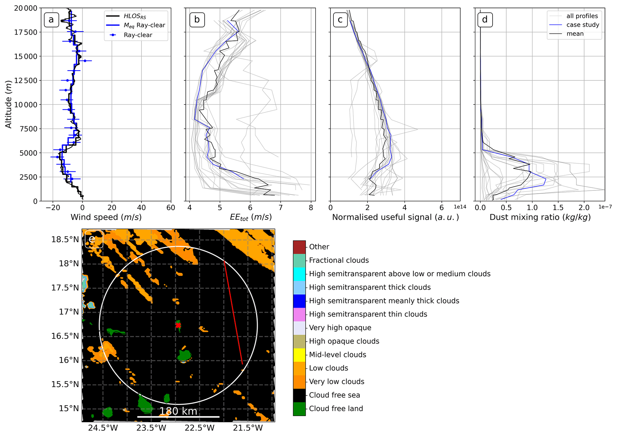
Figure 7 Overview of the cloud-free case study for a radiosonde launched from Sal Airport on 9 September 2021 at 18:45 UTC and the ascending orbit of Aeolus between 19:23:56 and 19:24:31 UTC for a co-location radius of 180 km. (a) Vertical radiosonde HLOS wind profile (solid black line) and projected onto Rayleigh-clear RBS (stepped black line), as well as averaged Rayleigh-clear observations (blue dots), corresponding EE_Aeolus (error bars), and ECMWF model equivalents (M_eq, stepped lines). (b) Vertical profile of the Rayleigh-clear EE_tot (blue line), together with the EE_tot of all 20 profiles described in Table 1 (solid grey lines) obtained from Eq. (9) and their average (solid black line). (c, d) Same as panel (b), but for normalised useful signal and CAMS dust mixing ratio, respectively. (e) Horizontal map showing the SAFNWC CT at 19:00 UTC and the co-location perimeter (solid white line), the Aeolus track (solid red line), and the radiosonde launch site (red cross). The cloud names follow the SAF NWC product nomenclature.

Figure 8 shows the same results as Fig. 7, but for cloudy conditions. In this case study, the radiosonde was also launched from Sal Airport, this time at 07:00 UTC on 14 September 2021, with a co-location radius of 60 km. Aeolus passed across the co-location region between 07:28:32 and 07:28:55 UTC, i.e. during the descending node. As can been seen in Fig. 8e, which corresponds to SAFNWC CT at 07:30 UTC, Aeolus passes over a variety of high clouds, mainly high semitransparent clouds. These high clouds appear to be located between 13 and 16 km altitude, as three Mie-cloudy (red) and two Rayleigh-cloudy (gold) observations are found in this range, and where the normalised useful signal is found to have a maximum. In this altitude range, all Rayleigh-clear, Rayleigh-cloudy, and Mie-cloudy observations exhibit good quality, with radiosonde observations generally within the error bars. Above this cloud cover at 16 km, we only find Rayleigh-clear observations that also perform well, with an EE_tot (Fig. 8b) and normalised useful signal (Fig. 8c) close to average. Beneath the cloud base at 13 km altitude, however, it appears that the Rayleigh-clear observations follow an irregular pattern, with most of the observations and error bars not matching the radiosonde observations, reaching deviations greater than 10 m s⁻¹. Accordingly, we find that the EE_tot (Fig. 8b) is larger in this altitude range mainly varying between 5 and 6 m s⁻¹, which also corresponds to a sharp decrease in the normalised useful signal well below the average (Fig. 8c). Nonetheless, the ECMWF model-equivalents in Fig. 8a remain fairly accurate relative to the radiosonde observations. This result mirrors the findings presented in the previous section, namely that the Rayleigh-clear EE_tot is systematically underestimated when the normalised useful signal is strongly attenuated. It appears that the normalised useful signal further decreases below 2.5 km, presumably as a result of the increasing dust concentration at this height (Fig. 8d), which most likely leads to a QC rejection of the Rayleigh-clear observations.

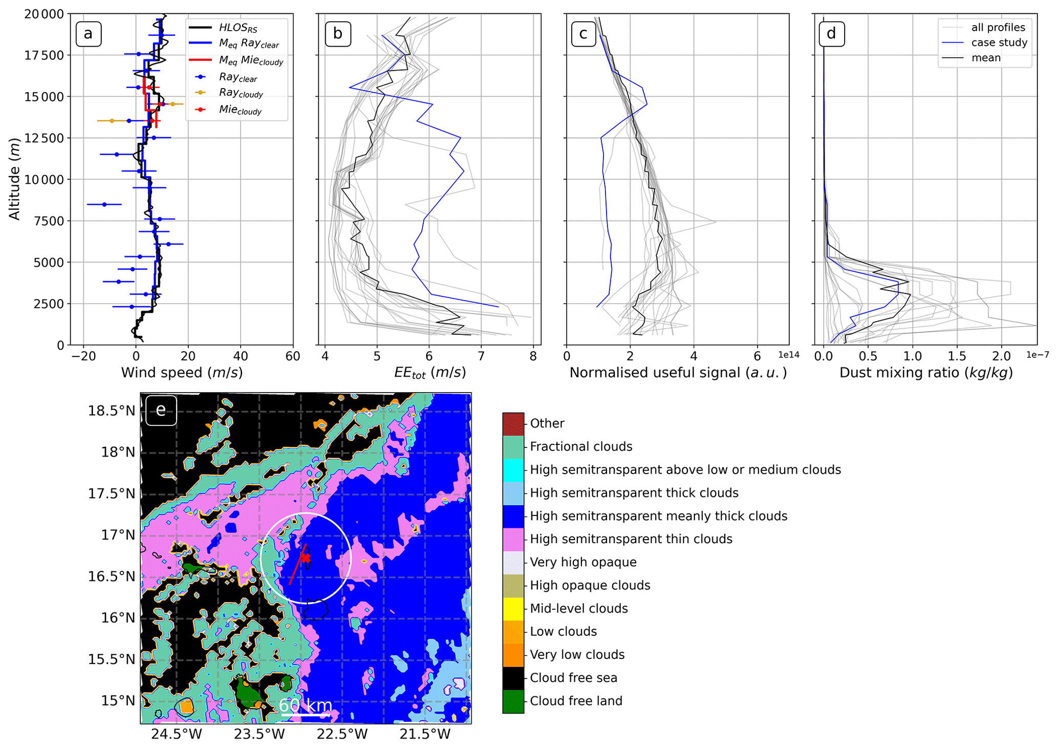
Figure 8 Same as Fig. 7, but for the case study with high cloud cover. Here, the radiosonde was launched from Sal Airport at 07:00 UTC on 14 September 2021, while Aeolus passed over the co-location area, with a radius of 60 km, on a descending node between 07:28:32 and 07:28:55 UTC. In panel (a), the red and orange colours represent the averaged Mie-cloudy and Rayleigh-cloudy observations (points), respectively, with the corresponding EE_Aeolus shown as error bars and ECMWF model equivalents (M_eq) shown as stepped lines. The SAFNWC CT shown in panel (e) corresponds to 07:30 UTC.

Lastly, Fig. 9 examines the influence of dust on the quality of Aeolus. In this case, the radiosonde was launched on 21 September 2021 at 06:50 UTC for a descending orbit of Aeolus, which passed over a co-location perimeter with a radius of 60 km between 07:28:44 and 07:29:07 UTC. As can be seen in Fig. 9e, the atmospheric conditions in the co-location area were completely cloud free at 07:30 UTC, with some low-level cloud further south of the island. The radiosonde profile shown in Fig. 9a indicates that Aeolus primarily measured in the Rayleigh channel along this orbital segment. Rayleigh-clear observations appear to be consistent with radiosonde wind observations throughout the mid-troposphere between 5 and 15 km altitude, while outliers with EEs of less than 5 m s⁻¹ (Fig. 9b) can be spotted above 15 km and below 5 km. This error structure is surprising, as both the normalised useful signal and error estimation curves are similar to those of the cloud-free case study in Fig. 7b and c. However, in Fig. 9d, we see that the Rayleigh-clear error pattern coincides with a strong peak in the dust mixing ratio, reaching more than $\mathrm{2}\times {\mathrm{10}}^{-\mathrm{7}}$ kg kg⁻¹ around 3.5 km altitude. The presence of dust seems to affect the quality of Rayleigh-clear observation without influencing the normalised useful signal and thus leading to an underestimation of the EE. The reason for this could be linked to a cross-talk.

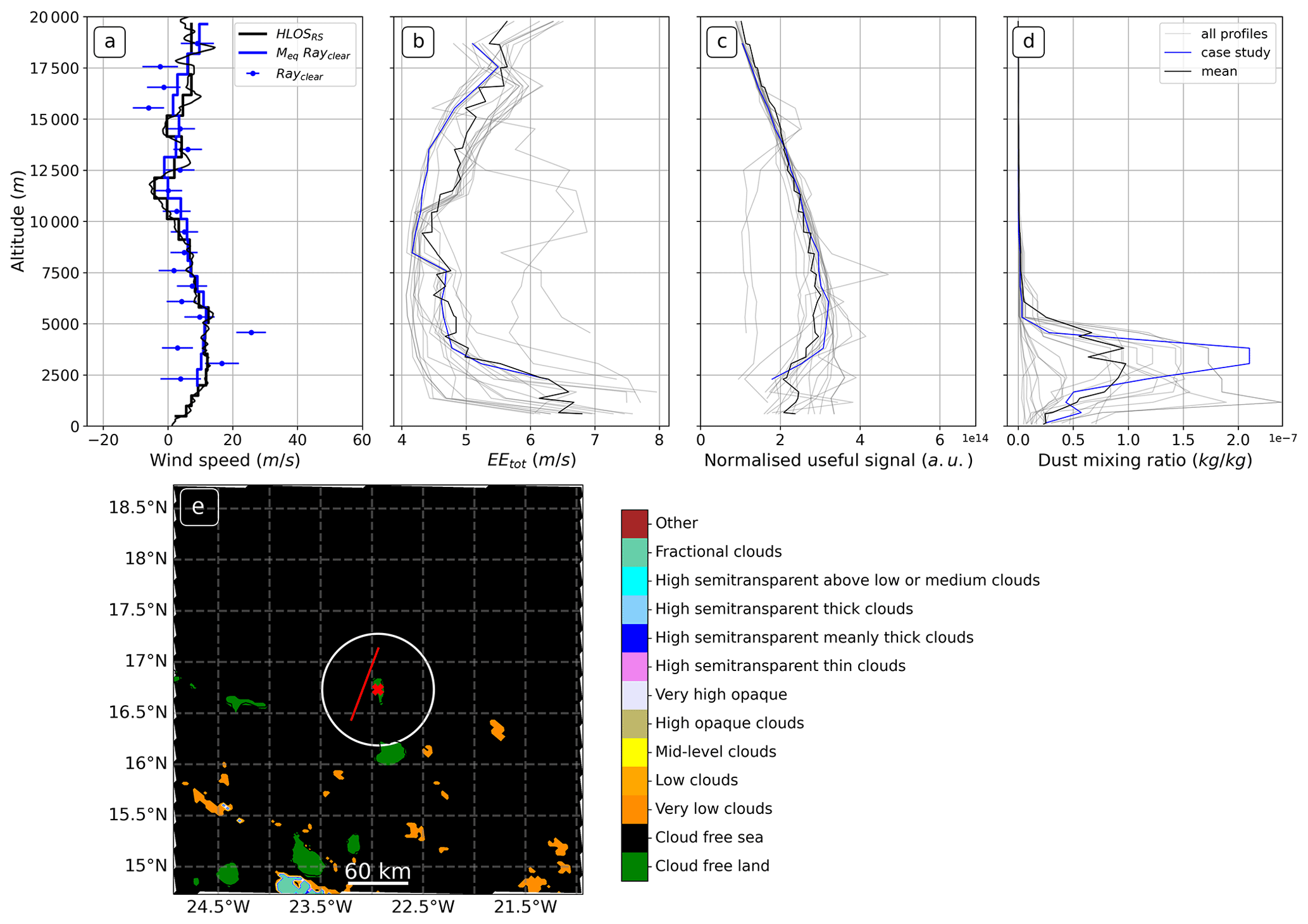
Figure 9 Same as Figs. 7 and 8 but for the case study with dust. Here, the radiosonde was launched from Sal Airport at 06:50 UTC on 21 September 2021, while Aeolus passed over the co-location area, with a radius of 60 km, on a descending node between 07:28:44 UTC and 07:29:07 UTC. The SAFNWC CT shown in panel (e) corresponds to 07:30 UTC.

5 Conclusions

In this study, we conducted a cross-Atlantic validation of Aeolus wind observations using radiosondes in the scope of the Joint Aeolus Tropical Atlantic Campaign (JATAC). Of the total 20 radiosonde profiles included in this work, 11 were launched from Puerto Rico and Saint Croix in the Caribbean and nine from Sal Airport on Cabo Verde between August and September 2021. The advantage of radiosondes is that they provide good vertical coverage, yielding 384 Rayleigh-clear bin-to-bin comparisons from the surface to an altitude of 20 km and 59 Mie-cloudy comparisons, mainly restricted to the presence of clouds and aerosols. After having applied several quality control (QC) and adaptation grid procedures, we quantified the quality of Rayleigh-clear, Mie-cloudy, and to a lesser extent Rayleigh-cloudy observation types, with respect to co-location aspects as well as atmospheric conditions such as cloud cover and dust concentration.

According to our statistical analysis, the total systematic error of Rayleigh-clear is $-\mathrm{0.5}\pm \mathrm{0.2}$ m s⁻¹, which is in agreement with the ESA recommendation of 0.7 m s⁻¹. The random error was calculated from the SD of the difference between radiosonde and Aeolus observations, accounting for radiosonde observation errors estimated at 0.7±0.28 m s⁻¹ and representativeness errors ranging from 1.5 to 2.5 m s⁻¹. In the altitude range of 2–16 and 16–20 km, the random error is 3.8–4.3 and 4.3–4.8, respectively, which is above the ESA-specified values of 2.5 and 3 m s⁻¹, respectively. In general, Rayleigh-clear shows no error dependency with respect to co-location radius, even for distances reaching 340 km, whilst being more sensitive to co-location time, especially if the radiosonde measurement is ahead of the Aeolus overflight time, which presumably corresponds to low-altitude observations. In addition, the systematic and random errors are height-dependent, with larger errors occurring in the upper troposphere, mainly caused by the reduction in signal return from decreasing air density, and in lower levels, most likely caused by the signal attenuation by clouds and dust. The EE likewise follows a similar form to the observed height error dependency, as it is inversely proportional to the square root of the normalised useful signal. In cases where the normalised useful signal is strongly attenuated by clouds or dust, the EE is generally underestimated, with observations exhibiting non-physical features and departures from radiosonde winds larger than the EE. A redefinition of the Rayleigh-clear EE could account for this underestimation by including other sources of noise, such as detector noise or readout noise, which increase for reduced signal levels. Furthermore, a cross-talk, i.e. the leakage of the Mie signal into the Rayleigh receiver, could also explain this underestimation, especially in the case of strong Mie returns. However, this supposition was not investigated in the context of this study. Outliers, defined as observations with small EE and large absolute differences, are found under all conditions, i.e. for all co-location radii, co-location times, altitudes, as well as cloud and dust cover. Their origin does not appear to be correlated with low signal levels but seems to be inherent to the statistical nature of the error distribution. Taking other terms into account when defining the EE, such as the influence of temperature, pressure, or SR on the Rayleigh response, could certainly contribute to improving the error characterisation. The ECMWF model equivalents of Rayleigh-clear are found to have a significantly better agreement with the radiosonde wind observations compared to the Rayleigh-clear observations. This is a further confirmation that the co-location parameters used for this validation study are appropriate and that the model equivalents provide a suitable reference for validating Aeolus. In addition, we demonstrate the existence of an orbital- and altitude-dependent bias in the Rayleigh-clear channel, which is visible with respect to both radiosondes and ECMWF model equivalents. This bias has already been documented by Borne et al. (2023) in West Africa using model equivalents and is now confirmed observationally. The underlying cause for this bias, however, remains unknown. In addition, we find that Rayleigh-clear performs better compared to Rayleigh-cloudy, but due to the lack of Rayleigh-cloudy data we cannot draw any strong conclusions.

For Mie-cloudy, the statistical analysis yielded a systematic negative deviation of $-\mathrm{0.9}\pm \mathrm{0.3}$ m s⁻¹ within ESA specifications when the standard error of the bias is taken into account, and it is consistent across all orbital nodes and Cal/Val sites. The random error between 2 and 16 km is 1.1–2.3 m s⁻¹, which falls within the ESA recommendations. The general quality of Mie-cloudy winds does not depend on the co-location radius, while it is more sensitive to temporal differences. The errors appear to be larger at 5 km and about 1 km altitude, typically at the upper and lower limits of the Saharan Air Layer, where clouds frequently occur. According to Lux et al. (2022a), the Mie fringe of the Fizeau interferometer can be distorted in the case of strong backscatter gradients, e.g. at cloud edges. Interestingly, Mie-cloudy does not seem to sample within dust layers, as most bins with high dust concentrations are rejected by the QC. Furthermore, the systematic and random Mie errors decrease with the percentage of cloud cover, while they increase in the presence of dust. This may be attributed to the generally weak backscatter of dust, increasing the error of the Mie-cloudy winds. Similar to Rayleigh-clear, outliers with small EE and large absolute differences can be found for all co-location distance, co-location time, altitude, dust concentrations, and cloud cover. An improvement of the Mie EE_Aeolus is expected from an optimisation of the Mie core algorithm, such as the fitting function or the classification algorithm.

The present study determined the error dependencies of the different Aeolus observation types and EEs with respect to tropical clouds and dust. The information acquired is valuable for further improvement of the processing algorithms in order to meet the requirements of the mission.