Post-process correction improves the accuracy of satellite PM_2.5 retrievals

Estimates of PM_2.5 levels are crucial for monitoring air quality and studying the epidemiological impact of air quality on the population. Currently, the most precise measurements of PM_2.5 are obtained from ground stations, resulting in limited spatial coverage. In this study, we consider satellite-based PM_2.5 retrieval, which involves conversion of high-resolution satellite retrieval of aerosol optical depth (AOD) into high-resolution PM_2.5 retrieval. To improve the accuracy of the AOD-to-PM_2.5 conversion, we employ the machine-learning-based post-process correction to correct the AOD-to-PM conversion ratio derived from Modern-Era Retrospective analysis for Research and Applications, Version 2 (MERRA-2) reanalysis model data. The post-process-correction approach utilizes a fusion and downscaling of satellite observation and retrieval data, MERRA-2 reanalysis data, various high-resolution geographical indicators, meteorological data, and ground station observations for learning a predictor for the approximation error in the AOD-to-PM_2.5 conversion ratio. The corrected conversion ratio is then applied to estimate PM_2.5 levels given the high-resolution satellite AOD retrieval data derived from Sentinel-3 observations. The region of study is central Europe during the year 2019. Our model produces PM_2.5 estimates with a spatial resolution of 100 m at satellite overpass times with R² = 0.55 and RMSE = 6.2 µg m⁻³. The corresponding metrics for monthly averages are R² = 0.72 and RMSE = 3.7 µg m⁻³. Additionally, we have incorporated an ensemble of neural networks to provide error envelopes for machine-learning-related uncertainty in the PM_2.5 estimates. The proposed approach can produce accurate high-resolution PM_2.5 data that can be very useful for air quality monitoring, emission regulation, and epidemiological studies.

1 Introduction

Poor air quality is one of the most serious environmental health risks of our time. In September 2021, the World Health Organization (WHO) released Global Air Quality Guidelines, revealing clear evidence of the damage air pollution inflicts on human health at even lower concentrations than previously understood (World Health Organization, 2021). The WHO estimates that exposure to air pollution causes 7 million premature deaths every year. A key indicator in monitoring air quality and epidemiological studies is the PM_2.5 parameter, which is the dry-mass concentration of fine particulate matter with an aerodynamic diameter of less than 2.5 µm (micrograms of particulate matter per cubic meter of air). Fine particulate matter originates from vehicle emissions, coal burning, and industrial emissions, among many other human and natural sources. Epidemiological studies link long exposures to high PM_2.5 levels to many severe illnesses, such as stroke and cardiovascular and respiratory diseases (e.g., Pope and Dockery, 2006; Cohen et al., 2017). On a global scale, the magnitude of the PM_2.5-exposure-related risk for human health is enormous as more than 90 % of the world's population lives in areas with annual mean PM_2.5 levels exceeding the new WHO 2021 air quality guideline of 5 µg per cubic meter (µg m⁻³, annual average) (Health Effects Institute, 2019).

While the knowledge of the health effects of pollution increases continuously, the epidemiological estimates still have significant uncertainties due to the lack of accurate global air pollution data (Hammer et al., 2020). Networks of ground-based observation stations produce accurate pointwise observations of PM_2.5 and certain chemical components such as ozone, sulfur dioxide, and nitrogen dioxide. These ground station measurements produce relatively accurate data, but the networks consist of only a few thousand irregularly located observation stations, mainly in developed countries, leading to the insufficient spatial coverage of the PM_2.5 data. To better monitor and understand air quality and pollution sources, near-real-time global observations of air quality are needed. The only way to get spatially resolved air quality data is to utilize satellite retrievals.

Satellite retrievals of PM_2.5 are often based on satellite aerosol optical depth (AOD) retrievals and an AOD-to-PM conversion ratio (Health Effects Institute, 2019; van Donkelaar et al., 2013; Zhang and Kondragunta, 2021; Geng et al., 2015). AOD is a columnar optical quantity, whereas PM_2.5 is the mass concentration of dry aerosol particles at some single point, typically at the surface level. Many factors affect the AOD-to-PM conversion ratio, including the aerosol vertical extinction profile, aerosol type and size distribution, and relative humidity. These factors are typically unavailable from a single data source, such as data provided by the instruments aboard a satellite, so a simulation-model-based AOD-to-PM ratio is often used. The simulation-model-based AOD-to-PM conversion ratio is typically computed based on meteorology, chemical transport models (CTMs), and auxiliary satellite data such as lidar-based aerosol vertical profiles. The PM_2.5 retrieval at a given location and time is then calculated as a product of the retrieved satellite AOD and the AOD-to-PM_2.5 ratio. The current state-of-the-art PM_2.5 retrieval algorithm also contains a post-processing step where the retrieved spatial PM_2.5 estimate is fitted to the ground-based PM_2.5 station data by a linear geographically weighted regression (van Donkelaar et al., 2016).

Many previous studies use machine-learning techniques to convert AOD to PM_2.5 levels. In particular, Ibrahim et al. (2022) used a variant of random forest called extremely randomized trees (ETs) to estimate PM_2.5 across Europe. Stafoggia et al. (2019) and Schneider et al. (2020) used random forest regressors in a multi-stage approach to estimate PM_2.5 at ground stations when only PM₁₀ measurements were available, to impute AOD values when not accessible, and to finally predict PM_2.5 values across Italy and Great Britain. Handschuh et al. (2023) considered multiple random forest models to evaluate PM_2.5 levels across Germany using four different AOD datasets.

In this paper, we propose a novel approach for high-resolution satellite-based retrieval of PM_2.5. While the previous studies use machine learning to learn the AOD-to-PM_2.5 conversion directly, we take a novel approach where we train the model to predict the approximation error in the geophysical-model-based conversion ratio. Our approach retrieves PM_2.5 at a spatial resolution of 100 m. It is based on the machine-learning post-process-correction approach, which we developed for the correction of approximation errors in satellite retrievals (Lipponen et al., 2021) and employed for high-resolution spectral aerosol optical depth (AOD) retrieval (POPCORN AOD) from Sentinel-3 SYNERGY data (Lipponen et al., 2022). In our algorithm development work, we take the spectral, high-resolution Sentinel-3 POPCORN AOD (Lipponen et al., 2022) as the starting point. Our PM_2.5 retrieval is based on the AOD-to-PM_2.5 conversion ratio applied to the POPCORN AOD. The AOD-to-PM_2.5 ratio is estimated by machine-learning techniques utilizing a fusion of collocated ground station-based in situ PM_2.5 data, MERRA-2 reanalysis model AOD and PM_2.5 data, spectral AERONET AOD, satellite-observed spectral top-of-atmosphere reflectances, meteorology data, and various high-resolution geographical indicators representing, for example, population density and land surface elevation. Utilizing these data, we employ the post-process-correction approach to the estimation of the AOD-to-PM_2.5 ratio (Lipponen et al., 2021, 2022; Taskinen et al., 2022), and then the high-resolution PM_2.5 retrieval is obtained as the product of the post-process-corrected AOD-to-PM_2.5 ratio and POPCORN AOD. Using an ensemble of neural networks, we can also provide error envelopes for the machine-learning-related uncertainty in the PM_2.5 estimates. The approach is tested with Sentinel-3 data from central Europe in 2019.

2 Data

We use various input data variables in computing the estimate for the surface PM_2.5. We use satellite observation data and retrievals, in situ observations, and reanalysis model data. This section lists all the variables and data sources used in our work.

2.1 Sentinel-3 POPCORN AOD

The Sentinel-3 POPCORN AOD product is based on the post-process-corrected Sentinel-3 SYNERGY land AOD product. It offers a spatial resolution of 300 m and is currently accessible for Sentinel-3A and 3B overpasses, covering five regions of interest for the year 2019: central Europe, eastern USA, western USA, southern Africa, and India. Two Sentinel-3 satellites currently flying provide revisit times of less than 2 d for the Ocean and Land Colour Instrument (OLCI) and less than 1 d for the Sea and Land Surface Temperature Radiometer (SLSTR) instrument at the Equator. The swath width of the OLCI instrument is 1270 km. The SLSTR swath width is 1420 km for the nadir view and 750 km for the oblique view.

The post-process correction is based on a feed-forward neural network that was trained to predict the bias in Sentinel-3 SYNERGY AOD. Sentinel-3–AERONET-collocated data were used as the training data for the neural network, and the trained neural network was then used for bias correction and super-resolution of the Sentinel-3 AOD (land) data. The idea for post-process correction of satellite AOD retrievals was introduced in Lipponen et al. (2021). For the technical details and accuracy metrics of Sentinel-3 SYNERGY land POPCORN AOD and related openly available code and data, see Lipponen et al. (2022).

In this work, we use POPCORN AODs at 440, 500, 550, 675, and 870 nm, as well as the Ångström exponent derived using AODs at these wavelengths as input for the AOD-to-PM_2.5 ratio model. POPCORN AODs are the data that bring the accurate AERONET AOD information to the AOD-to-PM_2.5 conversion.

2.2 OpenAQ

OpenAQ (https://openaq.org/, last access: 13 April 2023) is an open database for air quality data. In this work, we use OpenAQ as our data source for surface in situ PM_2.5 observations. OpenAQ provides pointwise air quality measurement data for thousands of stations. The temporal resolution of the data provided varies by station; 1 h and daily observations are commonly available. See Fig. 1 for a map of OpenAQ stations providing hourly data in our region of interest.

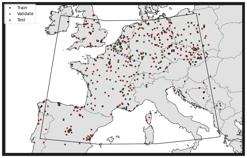
Figure 1 Map of stations in the region of interest.

Some OpenAQ stations report 24 h average PM_2.5 every hour.

In this work, we used the 24 h averages given every hour to estimate hourly PM_2.5. This was done station by station using a Tikhonov regularized (with regularization parameter value 0.05) least-squares fit to unfold the time-integrated data into hourly estimates.

In practice, the hourly PM_2.5 estimates were computed using the formula

$$\begin{array}{}\text{(1)}& {\mathrm{PM}}_{\mathrm{2.5},\mathrm{1}\mathrm{h}}={\left(A^{T}A+\mathit{\alpha }I\right)}^{-\mathrm{1}}{A}^{T}b,\end{array}$$

where

$$\begin{array}{}\text{(2)}& {\displaystyle }A=\left[\begin{array}{cccccccc}\frac{\mathrm{1}}{\mathrm{24}}& \frac{\mathrm{1}}{\mathrm{24}}& \mathrm{\cdots }& \frac{\mathrm{1}}{\mathrm{24}}& \mathrm{0}& \mathrm{0}& \mathrm{\cdots }& \mathrm{0}\\ \mathrm{0}& \frac{\mathrm{1}}{\mathrm{24}}& \mathrm{\cdots }& \frac{\mathrm{1}}{\mathrm{24}}& \frac{\mathrm{1}}{\mathrm{24}}& \mathrm{0}& \mathrm{\cdots }& \mathrm{0}\\ & & & \mathrm{⋮}& & & & \\ \mathrm{0}& \mathrm{0}& \mathrm{\cdots }& \mathrm{0}& \mathrm{0}& \mathrm{0}& \mathrm{\cdots }& \frac{\mathrm{1}}{\mathrm{24}}\end{array}\right],\text{(3)}& {\displaystyle }b=\left[\begin{array}{c}{\mathrm{PM}}_{\mathrm{2.5},\mathrm{24}\mathrm{h},\mathrm{1}}\\ {\mathrm{PM}}_{\mathrm{2.5},\mathrm{24}\mathrm{h},\mathrm{2}}\\ \mathrm{⋮}\\ {\mathrm{PM}}_{\mathrm{2.5},\mathrm{24}\mathrm{h},N}\end{array}\right],\text{(4)}& {\displaystyle }{\mathrm{PM}}_{\mathrm{2.5},\mathrm{1}\mathrm{h}}=\left[\begin{array}{c}{\mathrm{PM}}_{\mathrm{2.5},\mathrm{1}\mathrm{h},\mathrm{24}}\\ {\mathrm{PM}}_{\mathrm{2.5},\mathrm{1}\mathrm{h},\mathrm{25}}\\ \mathrm{⋮}\\ {\mathrm{PM}}_{\mathrm{2.5},\mathrm{1}\mathrm{h},N}\end{array}\right],\end{array}$$

and α is the regularization parameter. ${\mathrm{PM}}_{\mathrm{2.5},\mathrm{1}\mathrm{h},N}$ and ${\mathrm{PM}}_{\mathrm{2.5},\mathrm{24}\mathrm{h},N}$ denote the 1 and 24 h average PM_2.5 at time step N, respectively.

2.3 MERRA-2

The Modern-Era Retrospective analysis for Research and Applications, Version 2 (MERRA-2) is NASA's reanalysis model (Randles et al., 2017). MERRA-2 provides us meteorological variables, such as wind fields and temperatures. Furthermore, the MERRA-2 reanalysis also has the necessary aerosol and air quality information to compute an estimate for the surface PM_2.5.

MERRA-2 has a spatial resolution of 0.5° × 0.625°. This is roughly 50 km in the central Europe region. The time-varying MERRA-2 variables we use have the temporal resolution of 1 h, and instantaneous values or time-averaged values are given depending on the variable and data product. We also use some MERRA-2 constant variables as inputs for our AOD-to-PM_2.5 model. See the Appendix A for a list of all variables we have used as inputs in our models from the MERRA-2 reanalysis.

In addition to MERRA-2-provided variables, the following variables are derived using the MERRA-2 meteorology and aerosol-related variables and used in our models as inputs:

• relative humidity (RH) at the surface – equation based on the Clausius–Clapeyron equation (see e.g., Michaelides et al., 2019),

  $$\begin{array}{rl}\mathrm{RH}=& \mathrm{0.263}\cdot \mathrm{PS}\cdot \mathrm{QLML}/\\ & \exp \left((\mathrm{17.67}\cdot (\mathrm{T}\mathrm{2}\mathrm{M}-\mathrm{273.15}\left)\right)/(\mathrm{T}\mathrm{2}\mathrm{M}-\mathrm{29.65})\right);\end{array}$$

• wind direction (WD10M) at 10 m,

  $$\mathrm{WD}\mathrm{10}\mathrm{M}=\arctan \left(-\mathrm{V}\mathrm{10}\mathrm{M}/\mathrm{U}\mathrm{10}\mathrm{M}\right);$$

• wind speed (WS10M) at 10 m,

  $$\mathrm{WS}\mathrm{10}\mathrm{M}=\sqrt{\mathrm{U}\mathrm{10}{\mathrm{M}}^{\mathrm{2}}+\mathrm{V}\mathrm{10}{\mathrm{M}}^{\mathrm{2}}};$$

• PM_2.5 at surface (Buchard et al., 2016),

  $$\begin{array}{rl}{\mathrm{PM}}_{\mathrm{2.5}}& =\left(\mathrm{1.375}\cdot \mathrm{SO}\mathrm{4}\mathrm{SMASS}+\mathrm{1.4}\cdot \mathrm{OCSMASS}\right.\\ & +\mathrm{BCSMASS}+\mathrm{DUSMASS}\mathrm{25}\\ & \left.+\mathrm{SSSMASS}\mathrm{25}\right)\cdot {\mathrm{10}}^{\mathrm{9}};\end{array}$$

• AOD-to-PM_2.5 ratio η,

  $$\mathit{\eta }={\displaystyle \frac{{\mathrm{PM}}_{\mathrm{2.5}}}{\mathrm{TOTEXTTAU}}}.$$

2.4 CALIOP aerosol vertical profile climatology

We use the Cloud-Aerosol Lidar with Orthogonal Polarization (CALIOP) Lidar Level 3 Tropospheric Aerosol Profiles, Cloud Free Data, Standard Version 4-20 data product as one of our input data sources (NASA, 2022; Winker et al., 2010). This level 3 climatology data product has a spatial resolution of 2.5° × 2° and a temporal resolution of 1 month. We use daytime variables, and in the case of missing data, we use the nearest value found in the dataset. We use two variables from this dataset: AOD 63 % below and AOD 90 % below. These variables indicate the vertical height below which 63 % and 90 % of AOD is located on average. This gives us information about the vertical distribution of aerosols in the atmosphere.

2.5 Time variables

Information about the time of day and year is given as input for the model. The yearly and daily fractions from the beginning of the year and day until the end of year and day, respectively, are mapped to a unit circle, and the x and y coordinates of the unit circle points are used as inputs for the model. With this approach, we get very similar values for the end and beginning of the year and day.

2.6 High-resolution geographical indicators

2.6.1 OpenStreetMap roads

OpenStreetMap is an open-map project, and it contains map data with high spatial resolution. We use OpenStreetMap roads as a data source for our model inputs. We compute the distance to the nearest street or highway and use this distance as an input. We use a 100 m resolution grid for the distances. The paths, streets, and highways are all classified as “highways” in OpenStreetMap, and we use only the following sub-classes to only accept roads and highways with car traffic and thus potential PM_2.5 sources (information from OpenStreetMap, 2023). See Appendix A for all the OpenStreetMap road types used to compute the distance to the closest road.

2.6.2 NASA Black Marble night lights

NASA's Black Marble is a night light product based on Visible Infrared Imaging Radiometer Suite (VIIRS) day/night band (DNB) radiances measured at nighttime. DNB is highly sensitive to light and can therefore detect even very low intensity lights on Earth's surface at night. Most of the nighttime lights seen on Earth's surface are due to human activities. As human footprints are seen well in the night lights, we use the NASA Black Marble night lights as a proxy variable for the population density, and we use it as one input for our models. We use night light data at a spatial resolution of 500 m as our input based on the yearly data product VNP46A4 (Wang et al., 2020).

2.6.3 MODIS land cover type

We use the MODIS MCD12Q1 (Sulla-Menashe and Friedl, 2018) land cover type data product to derive input variables that contain distances to the closest International Geosphere-Biosphere Programme (IGBP) land cover types (Loveland and Belward, 1997; Belward et al., 1999). The spatial resolution of the MODIS MCD12Q1 data product is 500 m. For the list of IGBP land cover types, see Appendix A.

2.6.4 Digital elevation model

We use the Advanced Spaceborne Thermal Emission and Reflection Radiometer (ASTER) digital elevation model (DEM) to describe the land surface elevation (Fujisada et al., 2011, 2012; NASA et al., 2019). The ASTER DEM has a spatial resolution of 1 arcsec corresponding to about 30 m.

3 Methods

3.1 AOD-to-PM_2.5 conversion

For example, as in van Donkelaar et al. (2021), we model the dependency between the PM_2.5 at the surface level and AOD using the following model:

$$\begin{array}{}\text{(5)}& {\mathrm{PM}}_{\mathrm{2.5}}=\mathit{\eta }\cdot \mathrm{AOD},\end{array}$$

where $\mathit{\eta }=\mathit{\eta }(r,t)$ is the AOD-to-PM_2.5 conversion coefficient that is function of both time t and space r.

3.2 Post-process-correction approach

Let y∈ℝ^m denote an accurate satellite retrieval,

$$\begin{array}{}\text{(6)}& \mathit{y}=f\left(x\right),\end{array}$$

where vector y contains the output of the satellite retrieval algorithm, $f:{\mathbb{R}}^n\mapsto {\mathbb{R}}^m$ is an accurate retrieval algorithm, and x∈ℝⁿ contains all the algorithm inputs including the observation geometry and level 1 satellite observation data such as the top-of-atmosphere reflectances. The retrieval y can consist, for example, of surface PM_2.5 at a given point in space and time.

In practice, due to uncertainties in the auxiliary parameters of the underlying forward model, the extensive computational dimension of the problems, and processing time limitations, it is not possible to construct an accurate retrieval algorithm f, but an approximate retrieval algorithm,

$$\begin{array}{}\text{(7)}& \stackrel{\mathrm{̃}}{y}\approx \stackrel{\mathrm{̃}}{f}\left(x\right),\end{array}$$

has to be employed instead. The approximate retrieval $\stackrel{\mathrm{̃}}{f}$ is typically based on physically simplified and computationally reduced approximate forward models that are used due to the huge dimensionality of the retrieval problems and the need for computational efficiency. The utilization of the approximate retrieval algorithm leads to an approximation error,

$$\begin{array}{}\text{(8)}& e\left(x\right)=f\left(x\right)-\stackrel{\mathrm{̃}}{f}\left(x\right),\end{array}$$

in the retrieval parameters.

The core idea of the model-enforced post-process-correction model is to improve the accuracy of the approximate retrieval (7) by machine-learning techniques. By Eqs. (6)–(8), the accurate retrieval can be written as

$$\begin{array}{}\text{(9)}& \begin{array}{rl}\mathit{y}& =f\left(x\right)\\ & =\stackrel{\mathrm{̃}}{f}\left(x\right)+\left[f\left(x\right)-\stackrel{\mathrm{̃}}{f}\left(x\right)\right]\\ & =\stackrel{\mathrm{̃}}{f}\left(x\right)+e\left(x\right).\end{array}\end{array}$$

To obtain the corrected retrieval, Eq. (9) is used to combine the conventional (physics-based) retrieval algorithm $\stackrel{\mathrm{̃}}{f}\left(x\right)$ and a machine-learning-based model $\widehat{e}\left(x\right)$ to predict the realization of the approximation error e(x) to obtain a corrected retrieval

$$\begin{array}{}\text{(10)}& \mathit{y}\approx \stackrel{\mathrm{̃}}{f}\left(x\right)+\widehat{e}\left(x\right).\end{array}$$

Note that this approach is different from a conventional fully learned machine-learning model in which the aim is to emulate the accurate retrieval algorithm f(x) with a machine-learning model,

$$\begin{array}{}\text{(11)}& \mathit{y}\approx \widehat{f}\left(x\right),\end{array}$$

that is trained to predict the retrieval y directly from the satellite observation and geometry data x. The approximation error of the physics-based retrieval is a less complicated function (compared to the direct retrieval) for a machine-learning regression to learn. This leads to a more accurate and reliable estimation of the retrieval quantity.

3.3 Correction of AOD-to-PM_2.5 conversion factor η

In our work, we use the post-process-correction approach (10) to correct for the MERRA-2-based AOD-to-PM_2.5 conversion factor η. We utilize an ensemble of neural networks to learn the correction to the conversion factor η and simultaneously produce error envelopes related to the learning process. Our post-process-correction model $\widehat{e}\left(x\right):{\mathbb{R}}^n\mapsto \mathbb{R}$ corrects the conversion factor pixel by pixel, meaning that

$$\begin{array}{}\text{(12)}& {\displaystyle }\mathit{\eta }\left(x\right)=\widehat{\mathit{\eta }}+\widehat{e}\left(x\right),\text{(13)}& {\displaystyle }{\mathrm{PM}}_{\mathrm{2.5}}=\mathit{\eta }\left(x\right)\cdot {\mathrm{AOD}}_{\mathrm{POPCORN}},\end{array}$$

where $\widehat{\mathit{\eta }}$ represents the AOD-to-PM_2.5 ratio to be corrected. The correction model is learned using collocated data from ground station PM_2.5 data, MERRA-2 data, satellite data and retrieval, meteorological data, and high-resolution geographical indicators. All the inputs used can be found in Table A1 and are described in Sect. 2. We used SHAP analysis (Lundberg and Lee, 2017) in order to estimate feature importance after the training of the model. In Fig. A1 you can see a bar plot of the first 26 input features ordered by their importance (SHAP value), and in Table A1 the features are ordered by their SHAP importance (from left to right and from top to bottom). Since no features showed a non-negligible SHAP value, we decided to keep them all in the training of the model. We finally add the estimated correction term to the MERRA-2 η values and calculate the PM_2.5 estimates corresponding to POPCORN AOD retrievals using Eq. (5).

3.4 Selection of the network model

As the dimension n of the input data x to the correction model $\widehat{e}\left(x\right)$ is relatively small (n=172) and the output is a scalar, we utilize a fully connected feed-forward neural network for the regression task. The networks are implemented using the TensorFlow framework.

To optimize the neural-network architecture, we employed KerasTuner, a hyperparameter optimization framework. The Adam optimizer and 10⁻³ learning rate were selected. We used the mean square error (MSE) loss function in the training. A linear activation function was employed for the output layer as the correction $\widehat{e}\left(x\right)$ is real-valued. Other parameters, such as the activation functions and the number of nodes in hidden layers, were optimized using KerasTuner. We considered the number of hidden layers, experimenting with two-, three-, and four-layer architectures. The model with two hidden layers led to better accuracy compared to the deeper models with three or four hidden layers, and thus we employed the architecture with two hidden layers as our final model. The final optimal neural-network architecture is comprised of 172 input features and two hidden layers with seLu activation functions. The first and second hidden layers consist of 160 and 128 neurons, respectively. Figure 2 shows the neural-network architecture obtained from the model optimization.

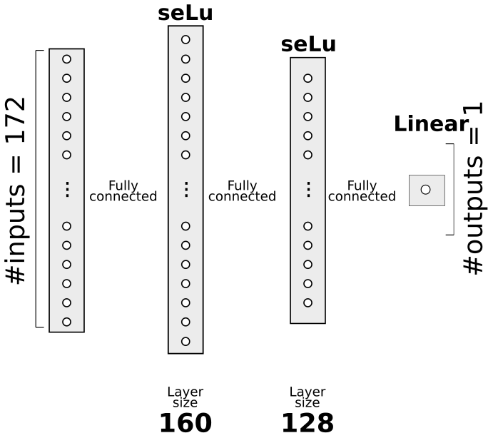
Figure 2 Feed-forward neural-network architecture for post-process correction of the η ratio, optimized with KerasTuner. The model contains two hidden layers with seLu activation functions (160 and 128 nodes, respectively) and a single node output layer with a linear activation function.

We divided the dataset into three subsets in training our neural-network model. Specifically, 60 % of the data were used for training, 20 % for validation, and 20 % for testing; see Fig. 1 for the division of the air quality (AQ) stations into the training, validation, and test sites. The learning data were divided into training, validation, and test data by stations instead of random division of data points in order to avoid model overfitting and having test data from locations within the region of interest that were not included in the model training. Figure 3 shows the proportions of different PM_2.5 values in the training, validation, and test data. We used the validation set and applied early stopping with a patience parameter value of 30 epochs to prevent the neural-network model from overfitting.

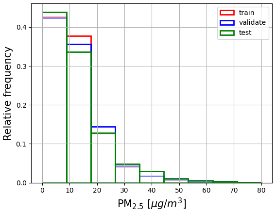
Figure 3 Distribution of AQ station PM_2.5 values in training, validation, and test sets. The training data are used to train the machine-learning algorithm, while the validation data are used to prevent overfitting. The test data are used to test the results after training. The division of the data was obtained by dividing the AQ stations in the region of interest into three separate sets with 60 %, 20 %, and 20 % shares of training, validation, and test stations.

In our tests, the model struggled to predict high PM_2.5 values accurately. We partially attributed this limitation to the skewed distribution of our dataset, which was predominantly composed of low PM_2.5 values; see Fig. 3 for the histogram of the PM_2.5 values of the AQ stations in the learning data. To address this, we introduced a cutoff value of 80 µg m⁻³ for PM_2.5 and trained our model with samples corresponding to PM_2.5 values only below this. Furthermore, we experimented with reweighting the loss function to emphasize higher PM_2.5 values. Although this strategy slightly improved the model's performance on the high-end tail, it compromised the accuracy on the low-end tail. Consequently, we decided not to use the reweighted loss function.

3.5 Ensemble of networks

To address the problem of local minima and dependency on the initialization in neural-network training, we used an ensemble-based technique where we trained an ensemble of 80 networks each initialized with different random weights. We considered the predictions of the networks as samples from a distribution and used the median of the predictions as a point estimate for the correction term of η. We use the spread minimum-to-maximum interval of the 80 outputs of the networks as a learning-related uncertainty for η, which was propagated onward to the uncertainty of the PM_2.5 estimates through the conversion (5).

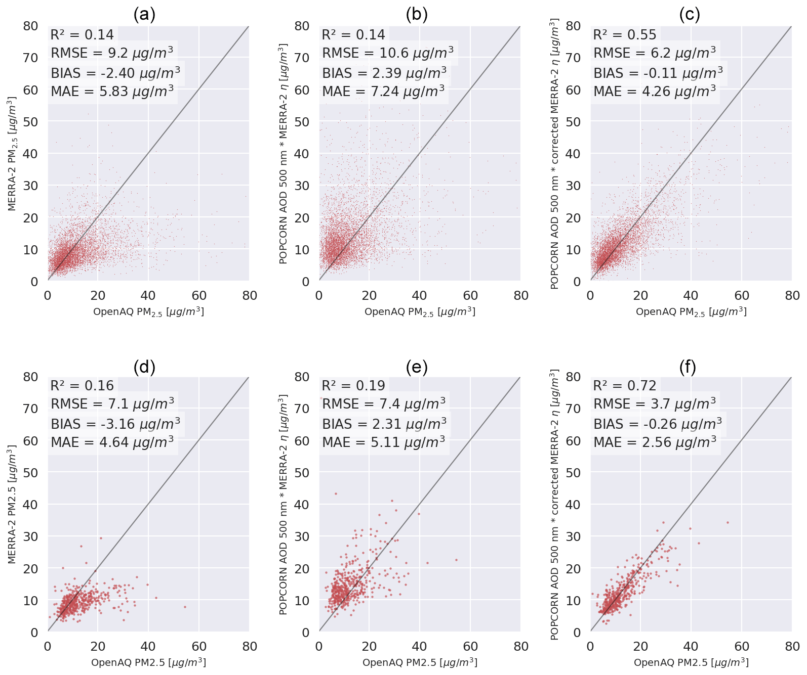
Figure 4 (a) MERRA-2 PM_2.5 predictions against OpenAQ PM_2.5 measurements per single overpass. (b) Uncorrected NOODLESALAD PM_2.5 predictions against OpenAQ PM_2.5 measurements per single overpass. (c) Corrected NOODLESALAD PM_2.5 predictions against OpenAQ PM_2.5 measurements per single overpass. (d) MERRA-2 monthly average PM_2.5 predictions against OpenAQ monthly average PM_2.5 measurements. (e) Uncorrected NOODLESALAD monthly average PM_2.5 predictions against OpenAQ monthly average PM_2.5 measurements. (f) Corrected NOODLESALAD monthly average PM_2.5 predictions against OpenAQ monthly average PM_2.5 measurements.

4 Results

Figure 4 shows scatter plots of the satellite- and model-based predictions of PM_2.5 with respect to the values of the ground stations for the test data AQ stations per single overpass and as monthly averages. We calculated the monthly averages considering a threshold: monthly averages were accepted only when we had more than five daily measurements per month (and station). The panels on the top row show results for single overpasses, and the panels on the bottom row show monthly averages. The panels on the left show the ground data comparison for the MERRA-2 PM_2.5 estimates, the panels in the middle show the ground data comparison for the PM_2.5 values estimated using Eq. (5) with POPCORN AOD and MERRA-2 conversion factor η, and the panels on the right show the comparison for the PM_2.5 values estimated using Eq. (5) with POPCORN AOD and post-process-corrected η. As can be seen, the use of a post-process-corrected conversion factor leads to a clear improvement on the accuracy of the predictions of PM_2.5 at the independent test data locations. The R² coefficient for instantaneous values is improved by about 290 % compared to both the MERRA-2 prediction and the estimate (5) with the POPCORN AOD and MERRA-2 conversion factor. The RMSE is improved by a factor of 32 % compared to MERRA-2 prediction and by a factor of 41 % compared to the product of POPCORN AOD with MERRA-2 η. The absolute value of the bias is reduced by a factor of over 95 % with respect to both of the uncorrected estimates, and the MAE decreased by a factor of 26 % compared to the MERRA-2 prediction and by a factor of 41 % compared to the product of POPCORN AOD with MERRA-2 η. In the monthly averages the R² coefficient is improved by a factor of 350 % with respect to MERRA-2 prediction and by a factor of 279 % compared to the estimate (5) with POPCORN AOD and MERRA-2 η. The RMSE in the monthly averages is reduced by a factor over 47 % with respect to both uncorrected methods. The bias in the monthly averages is reduced by a factor of 92 % and 89 %, respectively, and the MAE decreased by a factor of 44 % and 49 %.

We remark that we also tested the fully learned approach (11) for directly learning the AOD-to-PM_2.5 conversion factor η values instead of the correction of the MERRA-2-based conversion, but the results with the fully learned approach were less accurate than with the post-correction approach (10). The comparison can be seen in Fig. A2.

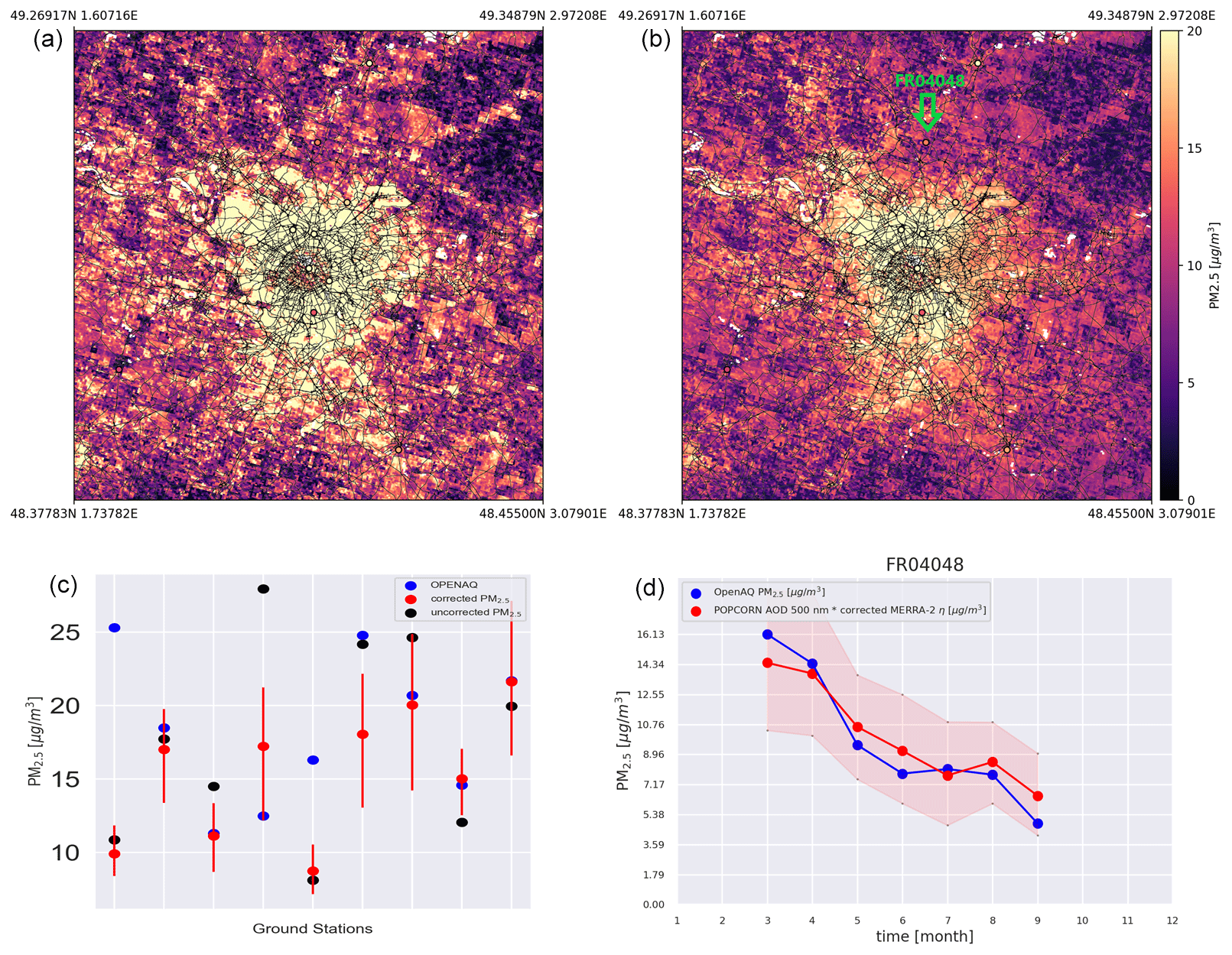
Figure 5 (a) Single-overpass not-corrected PM_2.5 map over Paris (RMSE against ground stations = 7.82 µg m⁻³). (b) Single-overpass corrected PM_2.5 map over Paris (RMSE against ground stations = 6.36 µg m⁻³). Notice that the white regions for the panels on top are regions where the AOD (so the PM_2.5) values are missing because of cloud contamination. (c) Comparison of the uncorrected and corrected method at the ground stations. The red error bars represent the spread of values obtained through the ensemble method, while the red dots represent the medians of those values. (d) Comparison between OpenAQ and corrected-method-predicted time series of PM_2.5 monthly averages at a single station (indicated on the corrected map by a green arrow). The red envelope represents the uncertainty coming from the ensemble method.

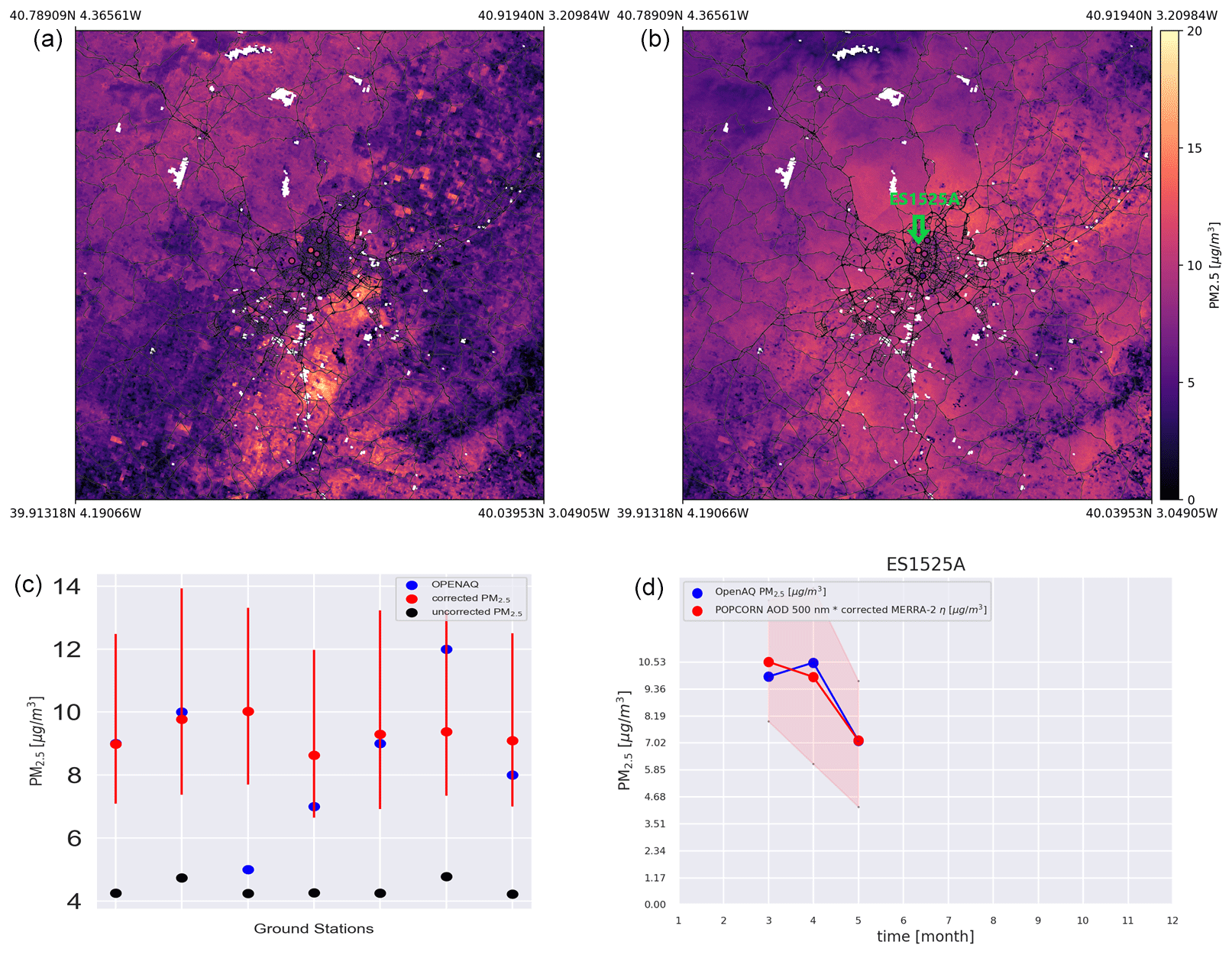
Figure 6 (a) Single-overpass not-corrected PM_2.5 map over Madrid (RMSE against ground stations = 4.59 µg m⁻³). (b) Single-overpass corrected PM_2.5 map over Madrid (RMSE against ground stations = 2.27 µg m⁻³). Notice that the white regions for the panels on top are regions where the AOD (so the PM_2.5) values are missing because of cloud contamination. (c) Comparison of the uncorrected and corrected method at the ground stations. The red error bars represent the spread of values obtained through the ensemble method, while the red dots represent the medians of those values. (d) Comparison between OpenAQ and corrected-method-predicted time series of PM_2.5 monthly averages at a single station (indicated on the corrected map by a green arrow). The red envelope represents the uncertainty coming from the ensemble method.

Figures 5 and 6 show PM_2.5 maps over Paris (23 February 2019) and Madrid (29 March 2019) for a single satellite overpass, respectively. On the top left the uncorrected map is obtained based on POPCORN AOD 500 nm and MERRA-2 η, while on the top right the corrected map uses the post-process-corrected MERRA-2 η. On the bottom left we compare the satellite-based PM_2.5 values to the measured PM_2.5 values at the AQ stations, which are represented by the circles in the maps. The red circles represent the post-corrected estimates (medians calculated from the ensemble predictions), the black dots represent the uncorrected estimates, and the blue dots represent the ground-based measurement values at the stations. The red error bars represent the spread of PM_2.5 values coming from the ensemble of networks, and they are to be considered uncertainty estimates related to the machine-learning process. The joint RMSEs of the uncorrected estimates with respect to the ground stations are 7.82 and 4.59 µg m⁻³, respectively, for Paris and Madrid, and the joint RMSEs for the post-corrected estimates with respect to the ground stations are 6.36 and 2.27 µg m⁻³, indicating improved accuracy of the per-overpass PM_2.5 estimates in the post-process-correction approach. Figures 5c and 6c reveal that, for all the stations, the different initialization points for the trainings improve over the uncorrected prediction. The median of the ensemble predictions is not always better than the uncorrected prediction, but the uncertainty interval either encloses the measured value or is closer to the measured value than the uncorrected estimate. The bottom-right images show a time series of PM_2.5 monthly average predictions against the time series coming from ground station monthly averages (the stations are shown on the corrected maps by a green arrow). The red envelopes show the uncertainty envelope of the post-process-corrected estimate. Here the ground station monthly averages are contained in the uncertainty envelope. Figure 7 shows time series of PM_2.5 monthly averages of the post-process-corrected estimates for different stations in the region of interest, showing good alignment with the accurate ground-based AQ measurements. Similar performance was found for the monthly averages in most of the test stations in the region of interest, indicating that the post-process-corrected estimates of monthly averages of PM_2.5 are generally well aligned with the accurate ground-based observations.

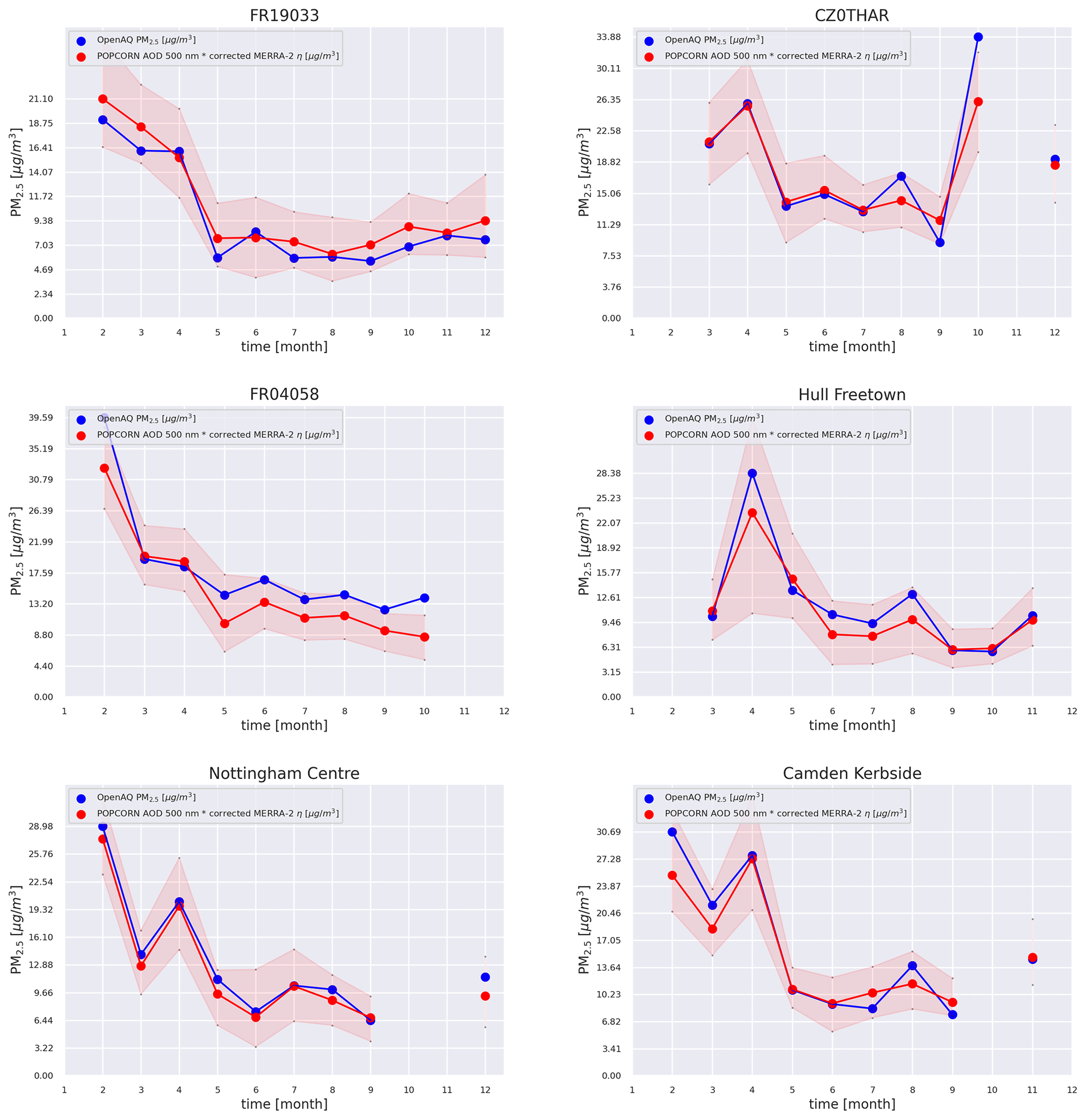
Figure 7 Monthly average time series for six stations from the independent test set within the region of interest. The red envelopes represent the uncertainty coming from the ensemble method.

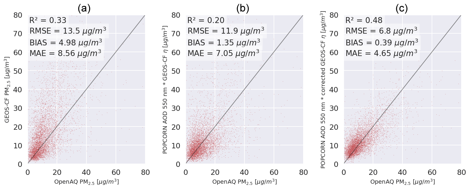
Figure 8 (a) GEOS-CF PM_2.5 predictions against OpenAQ PM_2.5 measurements per single overpass. (b) Uncorrected NOODLESALAD PM_2.5 predictions against OpenAQ PM_2.5 measurements per single overpass (using GEOS-CF data). (c) Corrected NOODLESALAD PM_2.5 predictions against OpenAQ PM_2.5 measurements per single overpass (using GEOS-CF data).

The post-process-correction method we have proposed here is flexible with respect to data utilized in the training, as it allows straightforward addition of more training data (by re-optimization of the neural-network architecture) coming from different data sources in order to improve the PM_2.5 predictions. In this study, we demonstrated the approach using POPCORN AOD data, which is obtained by post-correcting Sentinel-3 AOD. The approach can also be extended and trained to other satellite instruments and their AOD products to obtain similarly post-process-corrected high-resolution satellite estimates of PM_2.5, leading to more frequent temporal sampling of a particular location. In this study, we demonstrated the approach using a relatively large region of interest covering the year 2019 in central Europe. The approach can also be scaled in a straightforward manner to smaller or larger regions of interest by changing the training data. To demonstrate the performance of our approach with different model data, we tested the post-process correction using Goddard Earth Observing System Composition Forecast (GEOS-CF) data (Keller et al., 2021) instead of MERRA-2 data. GEOS-CF offers a higher spatial resolution of 25 km and variables that are not available from MERRA-2, for example, additional chemical species such as nitrate. The temporal resolution of GEOS-CF is 1 h. The result obtained when GEOS-CF data are used in the training of the correction model is shown in Fig. 8. Comparison to Fig. 4c shows that the performance of the correction model is similar to the model trained with MERRA-2 with MERRA-2, leading to slightly better error metrics.

5 Conclusions

We developed an innovative machine-learning technique aimed at correcting the AOD-to-PM_2.5 ratio derived from MERRA-2 data. This correction method integrates data from various sources, including ground station PM_2.5 data, MERRA-2 data, satellite data, meteorological data, and high-resolution geographical indicators. The post-process-corrected AOD-to-PM ratio was then employed to estimate PM_2.5 levels within the central Europe region for the year 2019. Our approach outperforms MERRA-2 predictions and predictions made using the MERRA-2 AOD-to-PM ratio and POPCORN AOD, resulting in an improvement in all evaluated metrics, whether considering individual overpasses or monthly averages. The PM_2.5 estimates were derived by aggregating the median values from an ensemble of neural networks. We incorporated the ensemble's value spread as a measure of machine-learning-related uncertainty in the post-process-corrected PM_2.5 estimates, and our estimates with their uncertainty envelopes were found to be generally highly feasible with respect to the accurate ground-based observations at the independent test station locations. We remark that while our approach produced generally good accuracy in estimation of PM_2.5, it exhibited poorer performance for the high-end values of PM_2.5. This finding can be attributed to the small number of learning data for the high-end tail of PM_2.5 values in our region of interest, highlighting the obvious fact that the learning data for machine learning need to be representative of the operational environment and conditions.

In this study, our goal was to utilize a simple neural-network model to estimate the PM_2.5 values from satellite data. Therefore, the adoption of a fully connected neural-network architecture was considered a reasonable choice. The architecture of the network was determined through a combination of manual selection and the use of KerasTuner to optimize the number of neurons per layer and the activation function. This ensured the development of an effective network for the specific problem under study. The robust performance of the resulting model highlights the efficacy of employing a simple neural-network model to address PM_2.5 estimation with notable success.

Appendix A: Lists of variables used from datasets

A1 MERRA-2 variables

We use the following meteorology-related variables from the MERRA-2 M2T1NXSLV dataset.

• PS: surface pressure (Pa)

• QV10M: 10 m specific humidity (kg kg⁻¹)

• QV2M: 2 m specific humidity (kg kg⁻¹)

• SLP: sea level pressure (Pa)

• T10M: 10 m air temperature (K)

• T2M: 2 m air temperature (K)

• TO3: total column ozone (dobsons)

• TOX: total column odd oxygen (kg m⁻²)

• TQI: total precipitable ice water (kg m⁻²)

• TQL: total precipitable liquid water (kg m⁻²)

• TQV: total precipitable water vapor (kg m⁻²)

• TROPPB: tropopause pressure based on blended estimate (Pa)

• TROPPT: tropopause pressure based on thermal estimate (Pa)

• TROPPV: tropopause pressure based on Ertel's potential vorticity (EPV) estimate (Pa)

• TROPQ: tropopause specific humidity using blended tropopause pressure (TROPP) estimate (kg kg⁻¹)

• TROPT: tropopause temperature using blended TROPP estimate (K)

• TS: surface skin temperature (K)

• U10M: 10 m eastward wind (m s⁻¹)

• U2M: 2 m eastward wind (m s⁻¹)

• U50M: eastward wind at 50 m (m s⁻¹)

• V10M: 10 m northward wind (m s⁻¹)

• V2M: 2 m northward wind (m s⁻¹)

• V50M: northward wind at 50 m (m s⁻¹)

We use the following meteorology-related variables from the MERRA-2 M2T1NXFLX dataset.

• BSTAR: surface buoyancy scale (m s⁻²)

• CDH: surface exchange coefficient for heat (kg m⁻² s⁻¹)

• CDM: surface exchange coefficient for momentum (kg m⁻² s⁻¹)

• CDQ: surface exchange coefficient for moisture (kg m⁻² s⁻¹)

• CN: surface neutral drag coefficient (1)

• DISPH: zero plane displacement height (m)

• EFLUX: total latent energy flux (W m⁻²)

• EVAP: evaporation from turbulence (kg m⁻² s⁻¹)

• FRCAN: areal fraction of anvil showers (1)

• FRCCN: areal fraction of convective showers (1)

• FRCLS: areal fraction of nonanvil large-scale showers (1)

• FRSEAICE: ice-covered fraction of tile (1)

• GHTSKIN: ground heating for skin temperature (W m ⁻²)

• HFLUX: sensible heat flux from turbulence (W m⁻²)

• HLML: surface layer height (m)

• NIRDF: surface downwelling near-infrared diffuse flux (W m⁻²)

• NIRDR: surface downwelling near-infrared beam flux (W m⁻²)

• PBLH: planetary boundary layer height (m)

• PGENTOT: total column production of precipitation (kg m⁻² s⁻¹)

• PRECANV: anvil precipitation (kg m⁻² s⁻¹)

• PRECCON: convective precipitation (kg m⁻² s⁻¹)

• PRECLSC: nonanvil large-scale precipitation (kg m⁻² s⁻¹)

• PRECSNO: snowfall (kg m⁻² s⁻¹)

• PRECTOT: total precipitation from atmospheric model physics (kg m⁻² s⁻¹)

• PRECTOTCORR: bias-corrected total precipitation (kg m⁻² s⁻¹)

• PREVTOT: total column re-evaporation or sublimation of precipitation (kg m⁻² s⁻¹)

• QLML: surface specific humidity (1)

• QSH: effective surface specific humidity (kg kg⁻¹)

• QSTAR: surface moisture scale (kg kg⁻¹)

• RHOA: air density at surface (kg m⁻³)

• RISFC: surface bulk Richardson number (1)

• SPEED: surface wind speed (m s⁻¹)

• SPEEDMAX: surface wind speed (m s⁻¹)

• TAUGWX: surface eastward gravity wave stress (N m⁻²)

• TAUGWY: surface northward gravity wave stress (N m⁻²)

• TAUX: eastward surface stress (N m⁻²)

• TAUY: northward surface stress (N m⁻²)

• TCZPBL: Transcom planetary boundary layer height (m)

• TLML: surface air temperature (K)

• TSH: effective surface skin temperature (K)

• TSTAR: surface temperature scale (K)

• ULML: surface eastward wind (m s⁻¹)

• USTAR: surface velocity scale (m s⁻¹)

• VLML: surface northward wind (m s⁻¹)

• Z0H: surface roughness for heat (m)

• Z0M: surface roughness (m)

We use the following aerosol- and air-quality-related variables from the MERRA-2 M2T1NXAER dataset.

• BCANGSTR: black carbon Ångström parameter 470–870 nm (1)

• BCCMASS: black carbon column mass density (kg m⁻²)

• BCEXTTAU: black carbon extinction AOD 550 nm (1)

• BCFLUXU: black carbon column u-wind mass flux (kg m⁻¹ s⁻¹)

• BCFLUXV: black carbon column v-wind mass flux (kg m⁻¹ s⁻¹)

• BCSCATAU: black carbon scattering AOD 550 nm (1)

• BCSMASS: black carbon surface mass concentration (kg m⁻³)

• DMSCMASS: DMS column mass density (kg m⁻²)

• DMSSMASS: DMS surface mass concentration (kg m⁻³)

• DUANGSTR: dust Ångström parameter 470–870 nm (1)

• DUCMASS: dust column mass density (kg m⁻²)

• DUCMASS25: dust column mass density – PM_2.5 (kg m⁻²)

• DUEXTT25: dust extinction AOD 550 nm – PM_2.5 (1)

• DUEXTTAU: dust extinction AOD 550 nm (1)

• DUFLUXU: dust column u-wind mass flux (kg m⁻¹ s⁻¹)

• DUFLUXV: dust column v-wind mass flux (kg m⁻¹ s⁻¹)

• DUSCAT25: dust scattering AOD 550 nm – PM_2.5 (1)

• DUSCATAU: dust scattering AOD 550 nm (1)

• DUSMASS: dust surface mass concentration (kg m⁻³)

• DUSMASS25: dust surface mass concentration – PM_2.5 (kg m⁻³)

• OCANGSTR: organic carbon Ångström parameter 470–870 nm (1)

• OCCMASS: organic carbon column mass density (kg m⁻²)

• OCEXTTAU: organic carbon extinction AOD 550 nm (1)

• OCFLUXU: organic carbon column u-wind mass flux (kg m⁻¹ s⁻¹)

• OCFLUXV: organic carbon column v-wind mass flux (kg m⁻¹ s⁻¹)

• OCSCATAU: organic carbon scattering AOD 550 nm (1)

• OCSMASS: organic carbon surface mass concentration (kg m⁻³)

• SO2CMASS: SO₂ column mass density (kg m⁻²)

• SO2SMASS: SO₂ surface mass concentration (kg m⁻³)

• SO4CMASS: SO₄ column mass density (kg m⁻²)

• SO4SMASS: SO₄ surface mass concentration (kg m⁻³)

• SSANGSTR: sea salt Ångström parameter 470–870 nm (1)

• SSCMASS: sea salt column mass density (kg m⁻²)

• SSCMASS25: sea salt column mass density – PM_2.5 (kg m⁻²)

• SSEXTT25: sea salt extinction AOD 550 nm – PM_2.5 (1)

• SSEXTTAU: sea salt extinction AOD 550 nm (1)

• SSFLUXU: sea salt column u-wind mass flux (kg m⁻¹ s⁻¹)

• SSFLUXV: sea salt column v-wind mass flux (kg m⁻¹ s⁻¹)

• SSSCAT25: sea salt scattering AOD 550 nm – PM_2.5 (1)

• SSSCATAU: sea salt scattering AOD 550 nm (1)

• SSSMASS: sea salt surface mass concentration (kg m⁻³)

• SSSMASS25: sea salt surface mass concentration – PM_2.5 (kg m⁻³)

• SUANGSTR: SO₄ Ångström parameter 470–870 nm (1)

• SUEXTTAU: SO₄ extinction AOD 550 nm (1)

• SUFLUXU: SO₄ column u-wind mass flux (kg m⁻¹ s⁻¹)

• SUFLUXV: SO₄ column v-wind mass flux (kg m⁻¹ s⁻¹)

• SUSCATAU: SO₄ scattering AOD 550 nm (1)

• TOTANGSTR: total aerosol Ångström parameter 470–870 nm (1)

• TOTEXTTAU: total aerosol extinction AOD 550 nm (1)

• TOTSCATAU: total aerosol scattering AOD 550 nm (1)

A2 OpenStreetMap road types used to compute the distance to the closest road

We use the following road types to compute the distance to the closest road. The descriptions of the road types are obtained from OpenStreetMap (2023).

• Motorway: a major restricted-access divided highway, normally with two or more running lanes plus an emergency hard shoulder; equivalent to the freeway, autobahn, etc.

• Trunk: the most important roads in a country's system that are not motorways.

• Primary: the next most important roads in a country's system.

• Secondary: the next most important roads in a country's system.

• Tertiary: the next most important roads in a country's system.

• Motorway_link: the link roads (slip roads/ramps) leading to/from a motorway from/to a motorway or lower-class highway; normally with the same motorway restrictions.

• Trunk_link: the link roads (slip roads/ramps) leading to/from a trunk road from/to a trunk road or lower-class highway.

• Primary_link: the link roads (slip roads/ramps) leading to/from a primary road from/to a primary road or lower-class highway.

• Secondary_link: the link roads (slip roads/ramps) leading to/from a secondary road from/to a secondary road or lower-class highway.

• Tertiary_link: the link roads (slip roads/ramps) leading to/from a tertiary road from/to a tertiary road or lower-class highway.

A3 IGBP land cover types

The IGBP classification contains the following land cover types:

1. evergreen needleleaf forests;

2. evergreen broadleaf forests;

3. deciduous needleleaf forests;

4. deciduous broadleaf forests;

5. mixed forests;

6. closed shrublands;

7. open shrublands;

8. woody savannas;

9. savannas;

10. grasslands;

11. permanent wetlands;

12. croplands;

13. urban and built-up;

14. cropland/natural;

15. snow and ice;

16. barren;

17. water bodies.

A4 Table of all input variables

Table A1 List of input variables used in our model ordered by SHAP value (from left to right and from top to bottom).

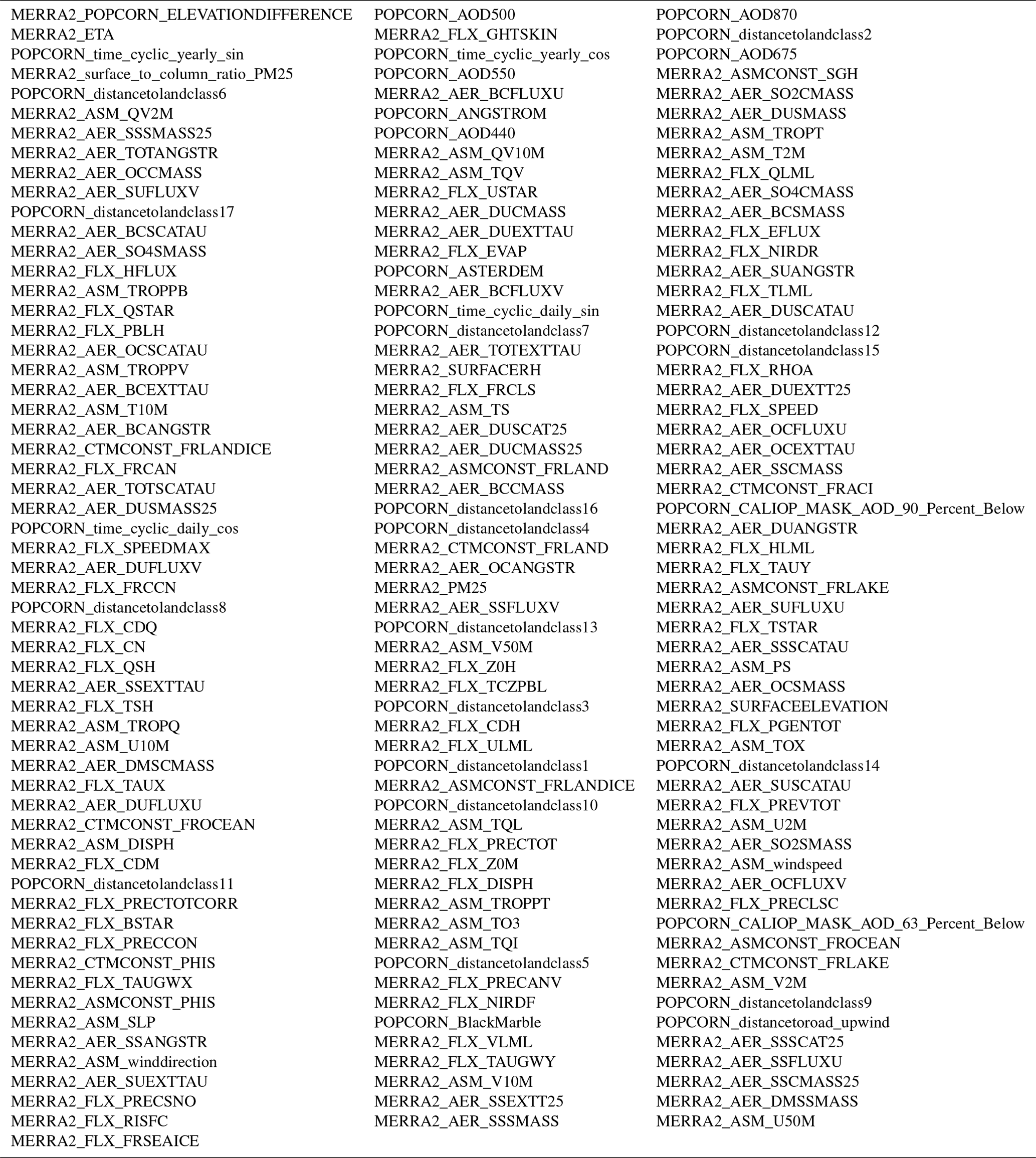
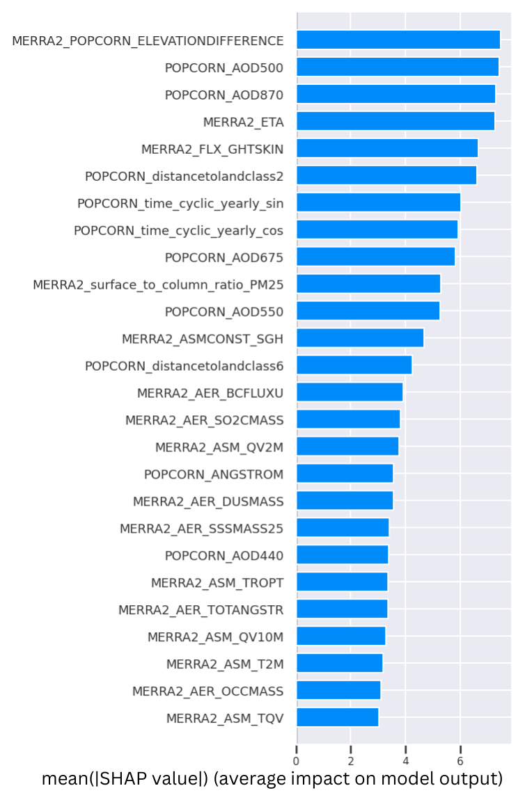
Figure A1 Bar plot of the SHAP values for the first 26 input variables in order of importance.

A5 Comparison of the post-process-correction approach vs. the fully learned approach

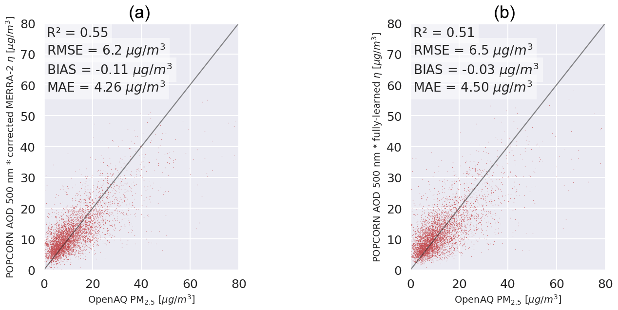
Figure A2 (a) Post-process-corrected PM_2.5 predictions against OpenAQ PM_2.5 measurements. (b) Fully learned NOODLESALAD PM_2.5 predictions against OpenAQ PM_2.5 measurements.