Validating global horizontal irradiance retrievals from Meteosat SEVIRI at increased spatial resolution against a dense network of ground-based observations

Accurate and detailed retrieval of global horizontal irradiance (GHI) has many benefits, for instance, in support of the energy transition towards an energy supply with a high share of renewable energy sources and for validating high-resolution weather and climate models. In this study, we apply a downscaling algorithm that combines the high-resolution visible and standard-resolution channels on board the Meteosat Spinning Enhanced Visible and Infrared Imager (SEVIRI) to obtain cloud physical properties and GHI at an increased nadir spatial resolution of 1 km × 1 km instead of 3 km × 3 km. We validate the change in accuracy of the high-resolution GHI in comparison to the standard-resolution product against ground-based observations from a unique network of 99 pyranometers deployed during the HOPE field campaign in Jülich, Germany, from 18 April to 22 July 2013. Over the entire duration of the field campaign, a small but statistically significant reduction in root mean square error (RMSE) of 2.8 W m⁻² is found for the high-resolution GHI at a 5 min scale. The added value of the increased spatial resolution is largest on days when GHI fluctuates strongly: for the 10 most variable days a significant reduction in the RMSE of 7.9 W m⁻² is obtained with high- versus standard-resolution retrievals. In contrast, we do not find significant differences between both resolutions for clear-sky and fully overcast days. The sensitivity of these results to temporal- and spatial-averaging scales is studied in detail. Our findings highlight the benefits of spatially dense network observations as well as a cloud-regime-resolved approach for the validation of GHI retrievals. We also conclude that more research is needed to optimally exploit the instrumental capabilities of current advanced geostationary satellites in terms of spatial resolution for GHI retrieval.

1 Introduction

In 2022, 46.1 GW of new solar photovoltaic (PV) capacity was installed within Europe, and the annually installed PV capacity is expected to continue to grow towards 120 GW in 2027 (SolarPowerEurope, 2023). On the global scale, solar PV is foreseen to account for half of all renewable power expansion between 2021 and 2026 (IEA, 2021). The eventual yield of these PV systems is dominated by occurring weather conditions. Scattering and absorption of incoming solar radiation by clouds and aerosols can lead to highly variable patterns of irradiance reaching the surface. This variability occurs at a wide range of temporal and spatial scales down to seconds and tens of metres (e.g. Madhavan et al., 2017; Damiani et al., 2018; Jiang et al., 2020; Habte et al., 2020; Mol et al., 2023) and is highly relevant to PV applications (Lohmann and Monahan, 2018). Apart from that, accurate observations of surface solar irradiance at high spatio-temporal resolution are also required for the evaluation of weather and climate models, in particular to assess whether the variability of radiation and thus clouds and aerosols is correctly resolved.

High-quality observations for studying cloud–radiation interactions can, for instance, be obtained from the Baseline Surface Radiation Network (BSRN) (Driemel et al., 2018), the Atmospheric Radiation Measurement (ARM) programme (Michalsky et al., 1999), or national measurement networks (e.g. Krähenmann et al., 2018). This mainly concerns point measurements, which provide a high temporal resolution but do not resolve the spatial distribution of global horizontal irradiance (GHI). Satellite data can be used to complement the sparse network of ground-based observations. Various algorithms have been developed to retrieve GHI from satellites (see Polo et al., 2016, for an overview).

In terms of temporal resolution, satellite retrievals of GHI do not match the ground-based observations (Polo et al., 2016). However, thanks to the coverage of large geographic areas and, in the case of geostationary satellites, the ability to resolve the complete diurnal cycle (e.g. Martins et al., 2016; Taylor et al., 2017; Seethala et al., 2018), satellite retrievals provide a unique source of data (Huang et al., 2019).

Over Europe and Africa, the Spinning Enhanced Visible and Infrared Imager (SEVIRI) on board the Meteosat Second Generation (MSG) weather satellites (Schmetz et al., 2002) measures spectral radiances in 11 narrowband channels at a subsatellite spatial resolution of 3 km × 3 km. Besides these 11 narrowband channels, SEVIRI has one high-resolution visible (HRV) channel with a 1 km × 1 km resolution. By incorporating the spatial information of the HRV channel in retrieval algorithms (downscaling), cloud properties and GHI can be retrieved at 1 km × 1 km instead of 3 km × 3 km resolution (Deneke et al., 2008; Werner and Deneke, 2020), hereafter called HR (high resolution) and SR (standard resolution), respectively.

This downscaling approach potentially offers an improved description of GHI and cloud variability. However, validation of a possible improvement of HR compared to SR GHI is not straightforward since it requires a specific set of ground-based observations to validate against. The density of ground-based pyranometers is normally too sparse to measure the small-scale spatial variability of GHI. High-quality pyranometer observations from adjacent stations are usually located in the order of 100 km from each other. Similar cloud conditions between these stations can therefore not be guaranteed. Studies that do measure spatial variability of GHI often focus on scales in the order of tens to hundreds of metres (e.g. Espinosa-Gavira et al., 2018; Silva and Brito, 2018; Järvelä et al., 2020). Though the smallest-scale variations of GHI are very relevant to PV applications (Gueymard, 2017; Kreuwel et al., 2020), these resolutions are too fine to validate the current SEVIRI downscaling algorithm. To demonstrate the SEVIRI spatial-resolution improvement from SR to HR, ideally, a network of observations covering an area of at least several pixels is used (Lorenzo et al., 2015; Yang, 2017). An additional constraint for the validation is that the ground-based observations need to be made within the disc of SEVIRI. The 2013 HOPE field campaign (Macke et al., 2017), where a network of 99 pyranometers (Lohmann et al., 2016; Madhavan et al., 2016) was set up in an area of 10 km × 12 km, meets these requirements. An exemplary comparison between SEVIRI GHI retrievals for a day with cumulus congestus was already presented by Deneke et al. (2021), showing that HR GHI compared better with the HOPE observations than SR GHI does. To our knowledge, a comprehensive assessment of changes in accuracy in GHI retrievals resulting from spatial-resolution improvements has not been carried out so far.

In this paper, we want fill this gap by extensively validating the downscaling algorithm of Deneke et al. (2021) against surface observations during the 2013 HOPE campaign. This study thus aims to assess whether and to what extent the smaller-scale spatial variability of GHI can be captured better by the HR retrieval. The validation is performed for a wide range of cloud conditions, allowing for the determination of the added value of the increased resolution for each of these cloud conditions.

The remainder of the paper is structured as follows. In Sect. 2, the ground-based and satellite datasets and the retrieval algorithm used in this study are introduced. ​​​​​​​Section 3 deals with the validation and identification methods for various cloud conditions. Results are presented in Sect. 4 and further discussed in Sect. 5. Conclusions and the outlook are presented in Sect. 6.

2 Data

This section describes the instruments and datasets we use to validate the downscaling algorithm. First, in Sect. 2.1, we introduce the HOPE campaign pyranometer network data in more detail. Here, we also discuss the quality screening applied to the pyranometer dataset. Next, the satellite data and retrieval scheme are described in more detail in Sect. 2.2.

2.1 HOPE campaign data

From 2 April to 24 July 2013, the High Definition Cloud and Precipitation for Advancing Climate Prediction (HD(CP)²) Observational Prototype Experiment (HOPE) field campaign took place. The HD(CP)² project aimed to improve the representation of cloud-precipitation processes within climate model simulations. As part of this project, the HOPE field campaign was executed with the specific purpose of providing a dataset which can be used for model evaluation at scales relevant to climate model simulations (Macke et al., 2017). During the HOPE campaign, 99 pyranometers were installed over an area of 10 km × 12 km (50.85–50.95° N, 6.36–6.50° E) near the German city of Jülich. The exact locations of the pyranometer stations are shown in Fig. 1. The land type around Jülich can mainly be identified as open farmland as well as some large open-pit mines. Each of the pyranometers was equipped with a silicon photodiode pyranometer of the model EKO ML-020VM to measure GHI at a 10 Hz resolution. The pyranometers were continuously operated during the entire length of the fieldwork. The pyranometer network and the resulting dataset have been described in Madhavan et al. (2016). While quality information based on manually recorded status information and visual checks is included in the original dataset, we perform an additional quality screening here to ensure that questionable data are omitted from the HOPE dataset.

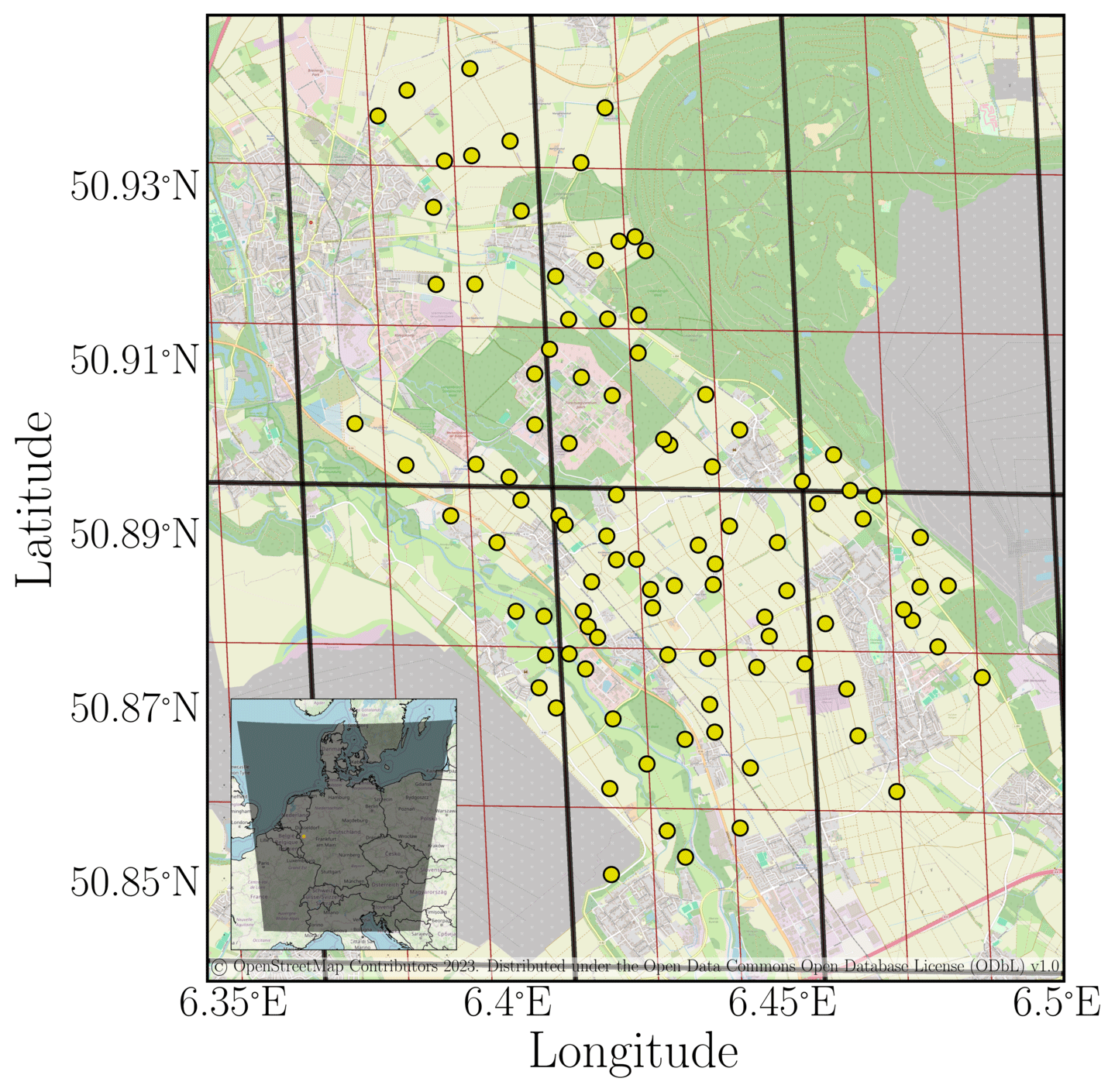
Figure 1 Locations of the 99 pyranometer stations set up during the 2013 HOPE field campaign near Jülich. The thick black lines indicate the edges of the SR pixels, whereas the thin red lines show the borders of the HR pixels. The subfigure in the bottom left corner illustrates the entire SEVIRI processing region used for this study. Map data: © OpenStreetMap contributors (2023). Distributed under the Open Data Commons Open Database License (ODbL) v1.0.

2.1.1 Quality screening

The first step in the quality control applied to the HOPE solar radiation measurements is a series of tests proposed by Long and Dutton (2002), which are widely used in the solar and radiation communities and in particular within BSRN (Driemel et al., 2018). The Long and Dutton (2002) quality control procedure is a set of tests applied to the global, direct, and diffuse irradiance measurement as well as a combination of the different components. Since only GHI has been measured during the HOPE campaign, only the extremely rare limit (ERL; Long and Dutton, 2002) test applying to GHI is used and given in Eq. (1):

$$\begin{array}{}\text{(1)}& -\mathrm{2}{\mathrm{W}\mathrm{m}}^{-\mathrm{2}}<\text{GHI}<\mathrm{1.2}\times \text{TOANI}\times {\mathit{\mu }}^{\mathrm{1.2}}+\mathrm{50}{\mathrm{W}\mathrm{m}}^{-\mathrm{2}}.\end{array}$$

In Eq. (1), TOANI is the top-of-atmosphere normal irradiance and μ is the cosine of the solar zenith angle.

An inspection of the measurements shows that many measurements whose values lie within the ERL range are not plausible, and, therefore, additional quality control is necessary. A visual inspection is undertaken to manually flag sensors for which a remaining measurement issue is suspected. In Appendix A, we further elaborate on the implementation of the visual inspection.

After performing quality control, we observe a daily reduction of roughly 5 % to 10 % in the number of valid sensors. To have a homogeneous number of sensors over the entire evaluation period, we have limited the range of the analysis to 18 April to 22 July 2013, instead of relying on the entire HOPE campaign period (ranging from 2 April to 24 July 2013).

2.2 Geostationary satellite data

In this study, we make use of the data from the MSG weather satellites operated by the European Organisation for the Exploitation of Meteorological Satellites (EUMETSAT). The MSG satellites are positioned in geostationary orbit. Four satellites were launched within this generation, Meteosat-8, Meteosat-9, Meteosat-10, and Meteosat-11, providing operational data since 2004. The SEVIRI instrument carried by MSG operates 12 spectral channels in the visible and infrared range of the spectrum. Here, we mainly consider the channels covering the visible-to-shortwave-infrared range of the spectrum (i.e. 0.6, 0.8, and 1.6 µm and the HRV channel), as these channels are the most relevant to deriving cloud properties and solar radiation products. The spectral bandwidth of the HRV channel is broader than for the 11 narrowband channels, ranging roughly from 0.4 to 1.1 µm. This study uses data from Meteosat-9, which was positioned at 9.5° E during the months of the field campaign. For some days during the campaign Meteosat-9 was not available. For these days, data from Meteosat-8 positioned at 3.5° E are used instead. Due to oblique viewing angles, the SEVIRI pixel size for the Jülich study domain is increased by about a factor 2 in the north–south direction compared to the pixel size at the subsatellite point. For the study domain, this means that each pixel covers an area of about 6.1 km × 3.2 km and 2.0 km × 1.1 km for the narrowband and HRV channels, respectively. The retrievals are only performed for a part of the SEVIRI disc, ranging from 44.4° N, 2.3° E to 57.8° N, 21.6° E, centred around Germany. This selected area consists of 240×400 SR pixels or 720×1200 HR pixels. The HOPE campaign area is covered by about 6 SR pixels and 31 HR pixels (see Fig. 1). Note that for the retrieval of satellite-derived GHI at the locations of the pyranometer stations, a collection of surrounding pixels is used, possibly including pixels that do not contain a pyranometer station (see Sect. 3.1). Using the rapid scanning service (RSS), only part of the SEVIRI disc covering northern Africa and Europe is scanned, enabling a 5 min repeat cycle. Until 2017, the Level 1.5 images of SEVIRI contained an erroneous georeferencing offset. SEVIRI pixels were shifted by 1.5 km in the northward and westward direction, resulting in an erroneous shift of 0.5 SR pixels and 1.5 HR pixels (EUMETSAT, 2017). We correct for this pixel shift to ensure accurate georeferencing in our analyses. The 0.6, 0.8, and 1.6 µm channels were calibrated following the methodology described in Meirink et al. (2013) by collocating and ray-matching reflectances from corresponding Moderate Resolution Imaging Spectroradiometer (MODIS) channels on the Aqua satellite. For other channels the operational calibration slopes were used, as provided in the SEVIRI Level 1.5 files.

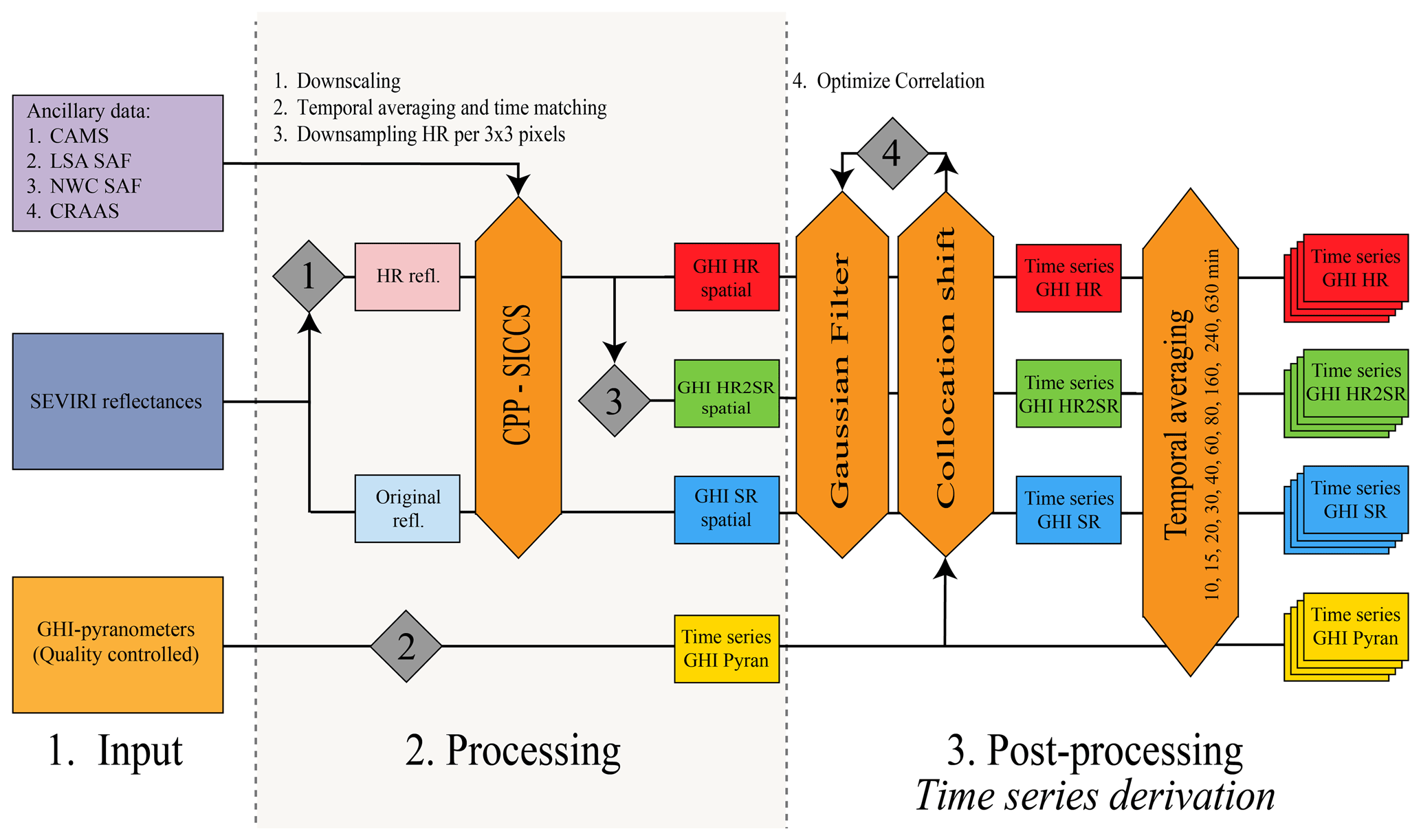
The following subsections summarize the processing scheme for retrieving cloud properties and GHI from SEVIRI radiances. An in-depth description of the entire workflow is presented in Deneke et al. (2021) and shown in a more compact form on the left hand side of Fig. 2.

Figure 2 Flow diagram illustrating the required steps to derive time series of GHI from SEVIRI reflectances. The input data and processing are explained in Sect. 2, while the post-processing is explained in Sect. 3, including an explanation of the CRAAS dataset and HR2SR product.

2.2.1 NWC SAF

As an initial step in the retrieval scheme, basic cloud properties are obtained by running the 2021 version of the Nowcasting and Very Short Range Forecasting Satellite Application Facility (NWC SAF) geostationary (GEO) software package (NWC SAF, 2021). The algorithm performs a series of spectral threshold tests on SEVIRI radiances to infer a cloud mask and determine the cloud type, cloud top temperature, and cloud top height. The NWC SAF software uses estimations of the atmospheric state from numerical weather prediction forecast and analysis fields, which have been retrieved from the ECMWF operational model archive.

2.2.2 Cloud Physical Properties (CPP)

To derive cloud optical and microphysical properties, the CPP algorithm (Roebeling et al., 2006; Benas et al., 2023) developed at the Royal Netherlands Meteorological Institute (KNMI) is used. The CPP algorithm starts with the determination of the phase (liquid or ice) near the cloud top, which is based on a modified version of the algorithm described in Pavolonis et al. (2005). Several spectral tests are performed on the observed brightness temperatures of the SEVIRI 6.2, 8.7, 10.8, 12, and 13.4 µm channels along with simulated brightness temperatures under clear and cloudy conditions, using the RTTOV v13 radiative transfer model (Saunders et al., 2018; Hocking et al., 2021). Next, reflectances from the SEVIRI 0.6 and 1.6 µm channels are used to simultaneously retrieve cloud optical thickness (COT) and effective radius (CER), following the principle of bi-spectral retrieval described in Nakajima and King (1990). This is done using precalculated look-up tables (LUTs), which have been generated with the Doubling Adding KNMI (DAK) radiative transfer model (de Haan et al., 1987; Stammes, 2001). CPP requires a number of inputs. Spectral surface reflectances are taken from the Land Surface Analysis Satellite Application Facility (LSA SAF; Carrer et al., 2018). Several atmospheric properties are required, including temperature and humidity profiles and the integrated ozone column, which are taken from the Copernicus Atmospheric Monitoring Service (CAMS) reanalysis and forecast (Inness et al., 2019). A comprehensive description of the retrieval scheme can be found in Benas et al. (2023) and CM SAF (2022).

2.2.3 Solar Irradiance under Clear and Cloudy Skies (SICCS)

The estimation of global, direct, and diffuse irradiance is performed by the SICCS algorithm using a second set of LUTs (Deneke and Roebeling, 2010; Greuell et al., 2013). These LUTs have been precalculated with a broadband version of the DAK model (Kuipers Munneke et al., 2008). In the LUTs, a distinction is made between cloud-free conditions and water or ice clouds. All LUTs take the solar zenith angle, broadband surface albedo (again from LSA SAF), integrated water vapour path, and ozone column into account. For clear-sky conditions, aerosol properties (optical depth, Ångström exponent, single-scattering albedo) and surface elevation serve as additional input parameters. Under cloudy conditions, COT and CER retrieved with CPP are considered instead. All atmospheric inputs are, as for CPP, taken from the CAMS reanalysis and forecast.

2.2.4 Downscaling

The description of the CPP–SICCS algorithm in the previous paragraphs relates to the retrieval at SR. Some additional steps are performed to generate GHI at high spatial resolution, starting with creating an HR cloud mask. Using the NWC SAF algorithm, we first generate a cloud mask at SR. However, this classification might lead to inaccuracies, especially in conditions with broken or factional clouds. Pixels that are identified as cloud filled at SR might be classified as partially cloud filled at HR (Werner et al., 2018). Here, we apply the updated HRV cloud masking scheme from Deneke et al. (2021), first introduced and described in detail by Bley and Deneke (2013). An HR cloud mask is derived by comparing the reflectances of the HRV channel to a clear-sky composite map generated from clear-sky HRV reflectances over 16 d. To identify the clear-sky pixels in the clear-sky composite map, we use an upsampled version of the NWC SAF cloud mask. Based on the calculation of the Matthews correlation coefficient (Matthews, 1975), for every HRV pixel, an optimal reflectance threshold is selected to separate clear from cloudy conditions. With the optimal reflectance thresholds, we construct the HR cloud mask from the HRV reflectances. The newly constructed HR cloud mask is then used as the new input for the HRV cloud masking algorithm to further optimize the separation between clear and cloudy pixels by repeating the algorithm for a few additional iterations.

To retrieve cloud properties at high spatial resolution, we utilize a modified version of the CPP retrieval. The HR retrieval relies on an assumed linear relation that links the 0.6 and 0.8 µm channels to the spectrally overlapping HRV channel (Cros et al., 2006; Deneke and Roebeling, 2010) as illustrated in Eq. (2):

$$\begin{array}{}\text{(2)}& \mathit{\delta }{r}_{\mathrm{06}}={\displaystyle \frac{\mathrm{1}}{a}}\left(\mathit{\delta }{r}_{\text{HV}}-b\mathit{\delta }{r}_{\mathrm{08}}\right).\end{array}$$

The linear relation from Eq. (2) does not apply to absolute values of reflectance but rather to the high-frequency residuals of the 0.6 µm, 0.8 µm, and HRV channels, denoted as δr₀₆, δr₀₈, and δr_HV, respectively. To determine the high-frequency residuals of the HRV channel, a modulation transfer function (MTF) is applied. The MTF filters out the HR spatial information (i.e. the scales between 1 and 3 km) from the HRV reflectances. Next, the filtered HRV reflectances are subtracted from the actual HRV reflectances to get the high-frequency residuals. In Eq. (2), a and b represent fit coefficients empirically determined by performing a least-squares regression on the assumed linear relationship between the residuals. More details on the determination of the fit coefficients and the application of the MTF can be found in Werner and Deneke (2020) and Deneke et al. (2021), respectively.

Equation (2) contains both δr₀₆ and δr₀₈ as unknowns. To solve Eq. (2), the assumption is made that, initially, δr₀₆ and δr₀₈ are equal, which enables us to make a first estimation of δr₀₆. The high-frequency residuals of the 0.6 µm channel are then added to the original 0.6 µm reflectances, providing updated values of reflectances for the 0.6 µm channel that include HRV information. Using CPP LUTs and the bi-spectral retrieval method of Nakajima and King (1990), COT can now be derived at HR. Next, the HR and SR COT are utilized in new retrieval iterations to retrieve an updated estimation of δr₀₈. With the new value for δr₀₈, Eq. (2) can be solved again to refine the estimation of δr₀₆ and accordingly provide an updated value for COT at HR. Neglecting the HR residuals of the r_1.6 micrometre channel reduces the accuracy of the CER retrieval compared to the SR retrieval. To restore the accuracy of the retrieved CER at HR, a local slope adjustment is performed. The slope adjustment determines where the high-frequency residual of r_1.6 equals zero, meaning the SR value of CER is restored. However, since the slope adjustment is based on the tangent of the COT contour at the location of the SR reflectances in the LUT, the HR CER retrieval does not precisely have to match the SR value (Werner and Deneke, 2020).

3 Methodology

This Methodology section is structured as follows. In Sect. 3.1, we present how the SEVIRI retrievals are validated against ground-based observations. Next, in Sect. 3.2, we introduce two methods to differentiate between various cloud conditions when performing the validation.

3.1 Validation

To validate the SEVIRI retrievals against ground-based observations, GHI time series are generated. The derivation of satellite-based time series is performed at the location of each of the 99 pyranometer stations, both at HR and SR. Besides the HR and SR SEVIRI GHI time series, an additional set of time series (HR2SR) are computed to study the effect of the downscaling algorithm in more detail. These time series are generated using the HR SEVIRI GHI but are averaged over 3×3 pixels to match the SR.

Following the method described in Greuell and Roebeling (2009), we account for the scale difference between the SEVIRI retrieval and the ground-based observations by smoothing the SEVIRI retrievals with a Gaussian filter (Eq. 3):

$$\begin{array}{}\text{(3)}& {\text{GHI}}_{t,n}={\displaystyle \frac{{\sum }_{i,j}{\text{GHI}}_{t,i,j}{e}^{-\frac{x_{i,j,n}^{\mathrm{2}}}{\mathrm{2}{\mathit{\sigma }}^{\mathrm{2}}}}}{{\sum }_{i,j}{e}^{-\frac{x_{i,j,n}^{\mathrm{2}}}{\mathrm{2}{\mathit{\sigma }}^{\mathrm{2}}}}}}.\end{array}$$

Here, ${\text{GHI}}_{t,i,j}$ is the retrieved GHI at pixel i,j and time t; GHI_t,n is the estimated satellite GHI at the location of station n at time t; and $x_{i,j,n}$ is the distance between the station n and the centre of SEVIRI pixel i,j. The Gaussian filter width σ is set to 1.0 km (Deneke et al., 2021).

The pyranometer network data are averaged to 5 min intervals to match the SEVIRI RSS temporal resolution. The 5 min averaging period is centred around the actual SEVIRI acquisition time for the Jülich area, which is about 3 min after the start time of the RSS scan.

In order to account for spatial mismatches between satellite and ground-based observations, a daily collocation shift is computed that maximizes the correlation between the ground-based observations and the satellite time series using the SEVIRI data between 06:15 and 17:15 UTC. For this procedure, shifts of the SEVIRI grid by multiples of 500 m in any direction are considered. The daily collocation shifts are then used to calculate a single collocation shift for the whole period of the HOPE campaign, which is based on the highest mean correlation over all the days. In this way, for the HR retrieval, a shift of the SEVIRI grid by 3.0 km south and 0.5 km east is obtained, while for the SR retrieval, a shift by 3.0 km south and 1.0 km east is found. With the collocation shift, we account for possible uncertainties due to inaccuracies and instabilities in the rectification to the SEVIRI grid as well as for parallax and shadow effects. Actual parallax and shadow displacements depend on cloud height and solar position and, therefore, vary between different pixels in the same image as well as between different satellite images. For the context of this study, however, we decided to keep a single offset for the whole period, since the mean optimal shift is indeed relatively constant throughout the study period: monthly averaged optimal shifts for HR and SR are within 1 km from the optimal shifts obtained for the whole period of the field campaign.

To validate the SEVIRI-derived GHI time series against the pyranometer network, for each of the 99 pyranometer stations, the root mean square error (RMSE) between the satellite-derived GHI and the ground-based GHI is computed. All observations from 18 April until 22 July 2013 between 06:15 and 16:45 UTC that have passed quality control are considered. To study the effect of temporal averaging, we repeat the original analysis with a 5 min temporal resolution for averaging times of 10, 15, 30, and 60 min. The results will be presented in box-and-whisker plots, where each box whisker represents 99 data points.

3.2 Scene identification

To differentiate between various cloud conditions we apply two methods: one based on the pyranometer network (Sect. 3.2.1) and one based on SEVIRI retrievals (Sect. 3.2.2).

3.2.1 Variability index

For the first method, based on the pyranometer network, we make a differentiation following the variability index (VI) method of Stein et al. (2012). This method relies on the calculation of the daily clearness index (DCI) and the variability index (VI). DCI is defined as the ratio between the daily summed GHI and the daily summed clear-sky irradiance (CSI). The values for CSI are taken from the CAMS McClear clear-sky model (Gschwind et al., 2019). VI is calculated as the ratio between the sum of the variations in GHI between consecutive time steps and the sum of the CSI variations between consecutive time steps for the same day (Δt) as defined in Eq. (4):

$$\begin{array}{}\text{(4)}& \text{VI}={\displaystyle \frac{{\sum }_{k=\mathrm{2}}^N\sqrt{({\text{GHI}}_k-{\text{GHI}}_{k-\mathrm{1}}{)}^{\mathrm{2}}+\mathrm{\Delta }{t}^{\mathrm{2}}}}{{\sum }_{k=\mathrm{2}}^N\sqrt{({\text{CSI}}_k-{\text{CSI}}_{k-\mathrm{1}}{)}^{\mathrm{2}}+\mathrm{\Delta }{t}^{\mathrm{2}}}}},\end{array}$$

where N is the number of time steps during a day. For each of the 99 pyranometer stations and every day of the HOPE field campaign, the DCI and VI are calculated. Next, for all the days, VI is normalized to the day with the highest VI to ensure that it ranges between 0 and 1. Finally, using the computed DCI and VI, four different cloud classes are determined: clear sky, overcast, highly variable, and mixed. The criteria for each of the four classes are shown in Table 1. The criteria are set so that the number of days in the clear-sky, variable, and overcast classes are equal. The distribution of the HOPE campaign days as a function of DCI and VI is illustrated in Fig. 3. High VI values characterize highly variable days regarding cloud conditions, whereas overcast and clear-sky days have a low VI. The separation between clear and overcast days is done based on the DCI, where clear-sky and overcast days have a high and low DCI, respectively.

Table 1 Criteria for division of the HOPE field campaign days into four variability classes using the variability index (VI) and daily clear-sky index (DCI).

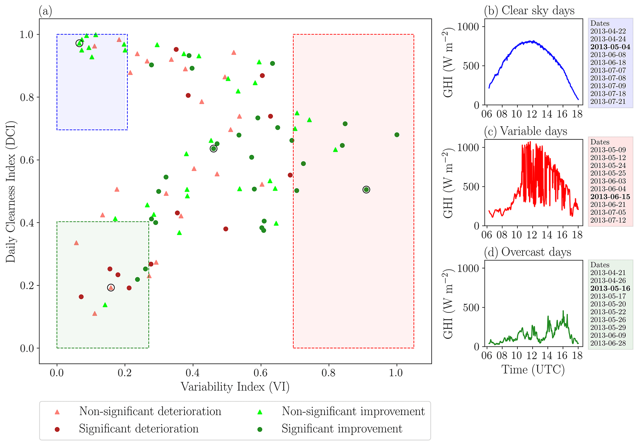
Figure 3 Variability index for the HOPE field campaign. (a) Scatterplot of DCI and VI: a single point represents 1 d of the campaign. The highly variable days fall within the red area, while the clear-sky and overcast days fall within the blue and green areas, respectively. All other dates are identified as mixed or partially variable. The points are colour-coded dependent on whether the downscaling algorithm yields a non-significant or significant deterioration or improvement. The scatter points marked with black edges represent the dates shown in Fig. 7. For the clear-sky, variable, and overcast days, an example of the development of GHI throughout the day is shown in panels (b), (c), and (d), respectively. Listed behind these GHI time series are the dates that fall within each of these categories, where the example dates are displayed in bold font.

3.2.2 CRAAS cloud regimes

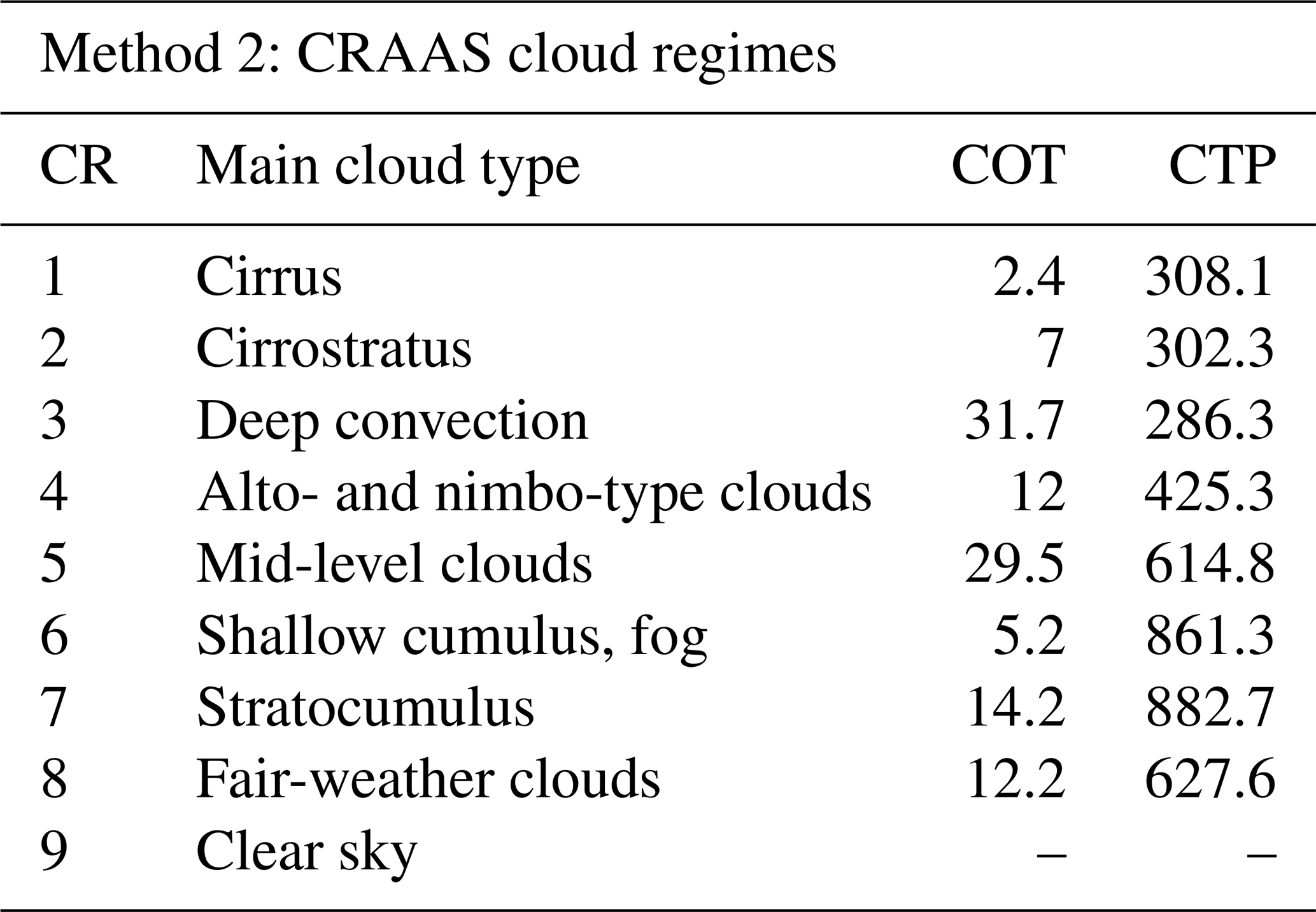
The satellite-based method for the determination of cloud conditions is based on the CRAAS European cloud regime dataset (Tzallas et al., 2022b). The CRAAS dataset uses the COT and cloud top pressure (CTP) taken from the CLAAS-2.1 dataset (Benas et al., 2017) to extract eight possible cloud regimes at a spatial resolution of 1° × 1° and 15 min intervals. The eight cloud regimes were determined by performing k-means clustering (Anderberg, 1973) based on the 2D histograms of COT and CTP. The eight cloud regimes and the corresponding main cloud types are summarized in Table 2 along with the mean values for COT and CTP for each of the regimes. Since no cloud regime is specified for clear-sky days, we take the clear-sky days as identified by the VI method and treat them as a separate clear-sky cloud regime (CR9).

Table 2 Classification of the eight CRAAS cloud regimes (CRs) and their associated main cloud types. The table includes median values of cloud optical thickness (COT) and cloud top pressure (CTP) for each cloud regime. We added a ninth regime consisting of the clear-sky dates from the variability index method.

4 Results

In this section, the results of the validation of the SEVIRI downscaling algorithm are presented. We first present the results without differentiating between cloud conditions (Sect. 4.1). Next, we show the results for subsets of the data derived with the VI method (Sect. 4.2). Then, four example cases are presented that illustrate the effects of the downscaling algorithm (Sect. 4.3). Finally, we show results for the CRAAS subsets to assess the added value of the HR product over the SR product under various cloud regimes (Sect. 4.4).

4.1 All conditions

When all dates of the HOPE field campaign are considered at a 5 min averaging time, we observe a decrease in median RMSE of 2.8 W m⁻² (or 2.8 %) if the HR product is used instead of the SR product (Fig. 4). This decrease is statistically significant according to the Mood median test (Mood, 1950).

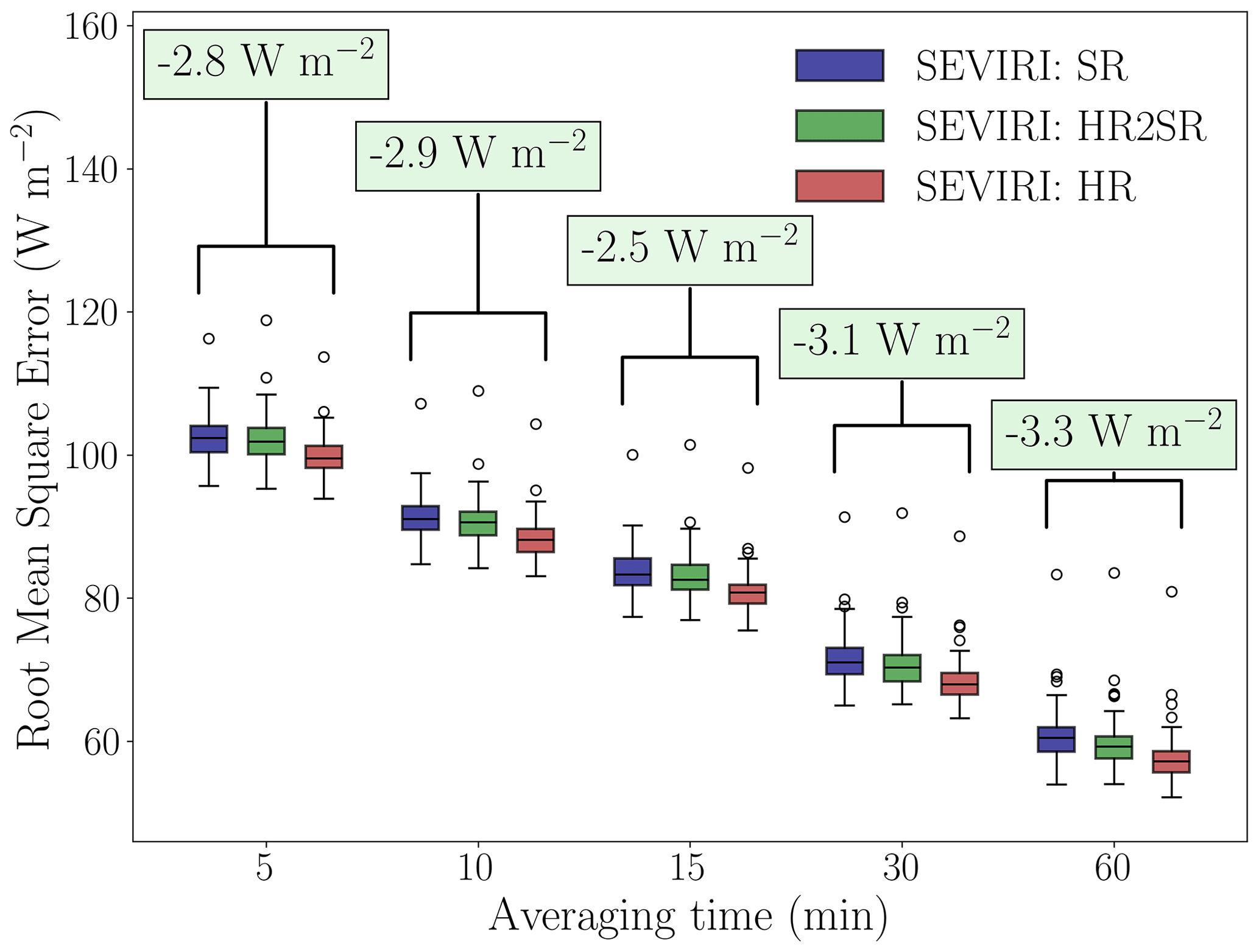
Figure 4 Box-and-whisker plots of the RMSE resulting from comparing the SEVIRI-derived and pyranometer-based GHI time series. Each boxplot is compiled from 99 data points representing the mean RMSE per station for all days between 18 April and 22 July 2013 from 06:15 until 16:45 UTC. Results are shown for the HR SEVIRI retrieval (SEVIRI: HR) and the SR SEVIRI retrieval (SEVIRI: SR), as well as for the HR SEVIRI retrieval that is spatially averaged to match SR (SEVIRI: HR2SR). These results are plotted for an averaging period ranging from 5 min to 1 h. The annotations above the boxplots show the median difference between the RMSE of the HR and SR retrievals. For all the averaging periods, the differences between HR and SR are significant at a 95 % confidence level according to the Mood median test, which is indicated by the continuous lines around the annotation boxes.

For the 5 min averaging time at a daily basis, we find an improvement of the HR product over the SR product for 60 out of 96 d, of which 27 are also statistically significant. For the remaining 36 d, no improvement is observed regarding the RMSE when the downscaling algorithm is applied. For 12 of these days, the deterioration is also statistically significant.

Comparison of the 3×3-pixel spatially averaged HR product (HR2SR) with the actual HR product confirms that the reduction in RMSE between HR and SR mainly results from the finer-scale spatial information contained in the HR retrieval. After spatial averaging, the largest part of the HR effect is removed. Minor differences that still occur between the 3×3-pixel spatially averaged HR retrieval and the SR product might be explained by differences between the SR cloud mask and the 3×3-pixel spatially averaged HRV cloud mask, which are not necessarily identical. Some HR information might still be included in the spatially averaged HRV cloud mask, and, therefore, a slightly lower RMSE may be observed for the 3×3-pixel spatially averaged HR retrieval than for the actual SR retrieval.

When the GHI time series are averaged over longer periods, as expected, a decrease in RMSE is observed since GHI variability is further averaged out both spatially and temporally. Moreover, even for these longer averaging times, the beneficial effect of the downscaling algorithm remains present. At hourly scales, the median HR benefit remains statistically significant and even larger than at the 5 min averaging time. The HR and SR errors for longer averaging times up to daytime averages (06:15–16:45 UTC) are discussed in more detail in Sect. 5.3.

In the results of Fig. 4 we have not differentiated between various cloud conditions. What we expect is that the effects of an improved resolution are most beneficial for variable conditions where smaller cloud structures can be resolved. From Fig. 3, we can derive that the beneficial effects of the downscaling algorithm do not remain limited to the most variable cases. Also, statistically significant improvements for the HR retrieval occur for less variable days.

4.2 Variability index classes

Using the variability index classification, we can further evaluate the possible added value of performing HR retrievals for the most persistent overcast, clear-sky, and highly variable days. For the days that are identified as clear sky, no significant difference between HR and SR is found (Fig. 5a). At a 5 min temporal resolution, the median RMSEs for HR and SR are 48.1 and 48.3 W m⁻², respectively. Under clear-sky conditions, no added value of the downscaling algorithm is expected because the satellite measurements are not used, and the only variability in the GHI retrieval is caused by the atmospheric composition (in particular aerosols and water vapour, based on numerical weather prediction – NWP – output at much coarser resolution). However, minor differences between both resolutions might arise from days identified as clear sky but still containing some clouds for a part of the day or from cloud-contaminated pixels that are only retrieved as cloudy at HR.

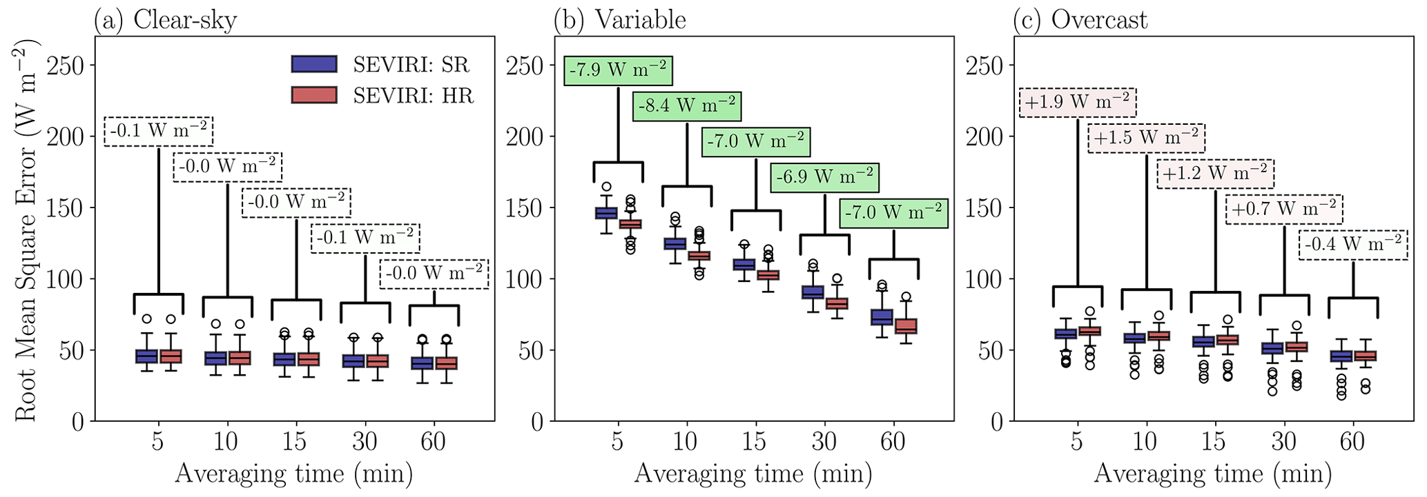
Figure 5 Box-and-whisker plots of the HR (SEVIRI: HR) and SR (SEVIRI: SR) RMSE between the SEVIRI-derived and pyranometer-based GHI time series, separated into three variability index classes: days falling in the clear-sky class are shown in panel (a), variable days in panel (b), and overcast days in panel (c). Averaging periods ranging from 5 min to 1 h are shown for each subplot. The annotations above the boxplots show the median difference between the RMSE of the HR and SR retrievals. Dotted lines around the annotation boxes indicate that the difference between HR and SR is non-significant at a 95 % confidence level according to the Mood median test, while continuous lines indicate a statistically significant difference between both resolutions.

The largest reductions in RMSE between both resolutions are found for days that are classified as highly variable (Fig. 5b). At a 5 min temporal resolution, the median reduction in RMSE between both resolutions is 7.9 W m⁻² (or 5.8 %). On these variable days, fast changes in cloud and radiation patterns occur, resulting in large overall errors. At a 5 min averaging time for both resolutions, the RMSE for the variable days is about 3 times as large as under clear-sky conditions. However, just as in Fig. 4, substantial reductions in RMSE are observed when longer averaging periods are considered. For the HR and SR retrieval, the median RMSE is halved when we use hourly averaged time series instead of the 5 min temporal resolution. The clear-sky (Fig. 5a) and overcast days (Fig. 5c) react much less strongly to the increasing averaging time, which is logical since surface radiation is both spatially and temporally less variable in these cases. Therefore, the decrease in RMSE observed for the longer averaging periods in Fig. 4 is mainly the result of a decrease in RMSE on the variable days.

Interestingly, when we apply the downscaling algorithm for the days that have been identified as overcast, we do not observe an improvement in accuracy (Fig. 5c). For the overcast cases, all averaging periods up to a 30 min averaging time show a small but non-significant increase in RMSE below 1.9 W m⁻², when the HR product is used instead of the SR product. Only for hourly averages, a non-significant improvement of 0.4 W m⁻² is found for the HR product. The days classified as overcast show the least variability in GHI from all dates of the HOPE field campaign. Therefore, it is likely that under these conditions, clouds are the most homogeneous regarding optical thickness and reflectance. We expect little added value from the downscaling algorithm for these conditions. On the other hand, a deterioration in accuracy is not expected either. In Sect. 5.2, we further elaborate on the performance of the downscaling algorithm for the most strongly overcast days.

In Fig. 6, we take a closer look at the errors made for the 10 highly variable days by splitting the GHI RMSE into bias and the standard deviation of the error (SDE) (SEVIRI minus pyranometer). The positive bias shown by both the HR and SR histograms indicates an overestimation of the SEVIRI retrieval with respect to the pyranometer network (Fig. 6, upper panels). However, even for clear-sky conditions, a positive bias is found (not shown). Since, for clear-sky conditions, the CPP–SICCS GHI retrievals solely depend on NWP output and are overall consistent with McClear estimates, there is probably an underestimation of the pyranometer network rather than an overestimation of the CPP–SICCS retrieval. Figure 6 also shows that for the 10 most variable days, mainly the SDE contributes to the total RMSE. Except for three pyranometer stations, applying the downscaling reduces both the bias and the SDE for each station in the order of 0 to 15 W m⁻². The downscaling also results in a slight increase in correlation with a median value just below 0.02.

Figure 6 Histograms of the bias (a) and standard deviation of the error (SDE) (c) between the SEVIRI-derived GHI at HR (red) and SR (blue) and the pyranometer observations for the highly variable days. The continuous black lines indicate the mean and standard deviation of the respective histograms. The dashed lines show the corresponding Gaussian distributions. Panel (b) shows the bias and SDE difference between HR and SR for each of the 99 pyranometer stations. The colour scaling in scatter points indicates the difference in correlation between HR and SR. The rhombus illustrates the magnitude of the median difference in SDE and bias. The black line in the colour bar shows the median HR correlation improvement.

4.3 Example cases

In Fig. 7, we plot the time series of GHI for both the HR and SR retrievals and the pyranometer network and relate these to the observed spatial distribution of GHI, cloud type, and properties retrieved with SEVIRI. We have selected four example cases, one from each VI class.

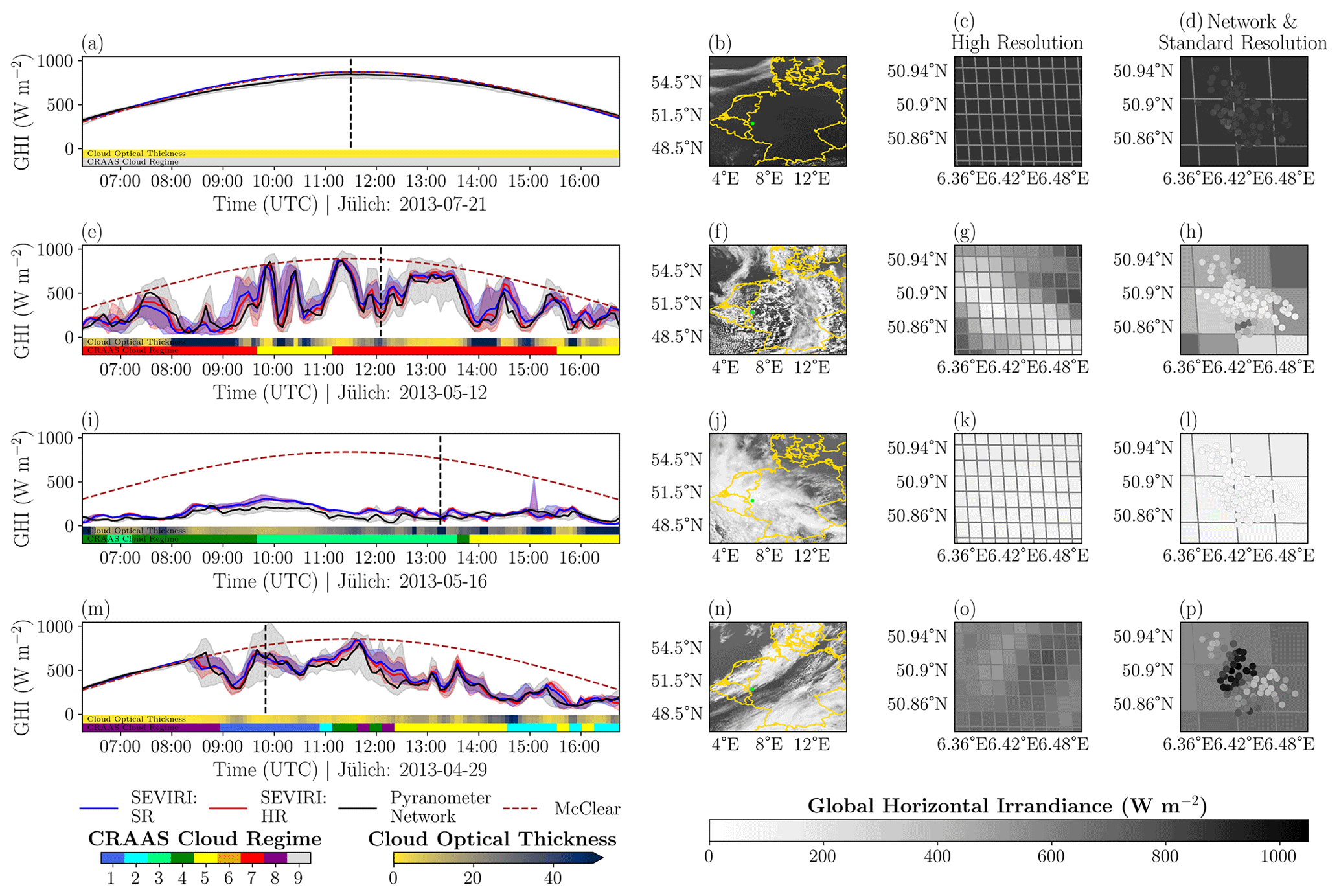
Figure 7 Time series (a, e, i, m) and the spatial distribution of global horizontal irradiance (GHI) over central Europe at HR (b, f, j, n) and the Jülich study domain at HR (c, g, k, o) and SR (d, h, l, p), respectively. The Jülich domain is highlighted in the central Europe domain plots by light-green pixels. Values of GHI for the pyranometer network have been plotted over the SR spatial plot. The vertical dashed black lines in the time series plots indicate the time of the spatial plots. The time series show the median GHI for a clear-sky (a), highly variable (e), overcast (i), and mixed (m) day at HR (red line) and SR (blue line) and for the pyranometer observations (black line). The colour-shaded areas show the data distribution between the 5th and 95th percentile. The dashed red lines show clear-sky irradiance simulated with the McClear clear-sky model. The colour bars below the time series indicate the cloud optical thickness and CRAAS cloud regime derived from the SEVIRI retrievals over the study domain.

The day of 21 July 2013 was selected to illustrate a clear-sky day. In fact, for large parts of central Europe, this was a persistently clear-sky day (Fig. 7a–d). Towards the afternoon, some cumulus developed in northern France, Luxembourg, and Belgium (not shown). However, these clouds did not reach the Jülich study domain. The GHI time series show an identical retrieval for HR and SR throughout the entire day. This is as expected since the lack of clouds means that the retrieval solely relies on NWP output, which is identical for both resolutions. Also, the pyranometer network observations show a comparable parabolic GHI development. However, especially in the hours leading up to noon, lower clear-sky irradiance is measured with the pyranometer network than with the SEVIRI retrievals. Furthermore, some spread in GHI can be observed between the different pyranometer stations, likely caused by slight tilts of the instruments and imperfect calibration.

The day of 12 May 2013 was one of the most variable days during the HOPE field campaign in terms of radiation variability. Over the whole day, strong fluctuations in GHI were measured (Fig. 7e–h). Using the HR retrieval, especially the dips in GHI are better represented, which contributes to a significant improvement in accuracy as shown in Fig. 5b.

The pyranometer observations show that cloud enhancement, i.e. GHI exceeding clear-sky GHI, occurs at multiple moments throughout this day. From surface observations, it is known that especially for altocumulus, cloud enhancement can be prominent, with GHI even exceeding its clear-sky value by up to 40 % at subminute timescales (Mol et al., 2024). Here, the observed cloud enhancement is smaller since, in this study, 5 min averaged observations of GHI are considered and the effects of cloud enhancements are more pronounced at smaller timescales. The CPP–SICCS retrieval cannot derive cloud enhancements as the algorithm relies on 1D radiative transfer. Therefore, the maximum GHI retrieved with SEVIRI is limited to the clear-sky value, as can be seen at 09:50 UTC.

Despite the lack of cloud enhancement in the SEVIRI retrieval, for large parts of the day, the spread in GHI retrieved with SEVIRI matches the observed GHI variability between the pyranometer stations rather well. This might indicate that, at those moments, the subpixel variability of GHI remains limited and clouds appear over the study domain with sizes that SEVIRI can capture. However, there are also periods, e.g. between 12:30 and 13:30 UTC, when the satellite-retrieved spatial GHI variability is much smaller than indicated by the pyranometer observations. From the spatial plot at HR, we can clearly distinguish the transition between cloudy and clear-sky regions. This is harder to detect at SR since a much less smooth cloud edge is retrieved. This example illustrates that the HR retrieval not only is able to resolve smaller clouds themselves but is also able to resolve finer cloud structures in larger cloud systems.

As an example of an overcast day, we show the time series for 16 May 2013 (Fig. 7i–l). This day was persistently cloudy with relatively thick, high-level clouds (CRAAS regimes CR3–CR5). The GHI observed with the pyranometer network does not reach values above 250 W m⁻² throughout the entire day. The limited spread in GHI between the pyranometer stations indicates homogeneous cloud conditions, as illustrated by the spatial distribution of GHI, where little variation can be seen. In the early afternoon, some fluctuations in GHI can be observed from the SEVIRI retrieval, corresponding to sudden changes in COT. These fluctuations are observed to a much smaller extent by the ground-based measurements. Furthermore, on most of the overcast days, we observe a slightly more strongly fluctuating GHI signal for the HR retrieval than for the SR retrieval. These differences and a possible explanation are discussed in more detail in Sect. 5.2.

Finally, we have selected 29 April 2013 to illustrate a day classified as mixed using the VI method (Fig. 7m–p). This day started off with clear skies, but from 08:30 UTC onward, various cloud types moved over the Jülich domain. Throughout the day, the COT gradually increased. Both the HR and SR retrieval can capture the mean observed GHI from the pyranometer network well. On this date, the spread in GHI between the different pyranometer stations strongly varies. In the morning, there is a large spread between the different pyranometer stations, while, in the afternoon, the spread between the pyranometer stations remains limited. For both SEVIRI retrievals, the spread in GHI between the pixels is relatively constant. Therefore, only in the afternoon do the SEVIRI retrievals represent the observed spatial variability in GHI well. The large spread in GHI observed by the pyranometer network in the morning, which is not captured by SEVIRI retrievals, indicates a situation where clouds occur at a subpixel scale that SEVIRI cannot resolve at either resolution. From the spatial plots of the pyranometer network, we can distinguish two cloudy regions in the eastern and northwestern part of the domain, with in-between clear-sky conditions. Considerable cloud enhancement occurs in this clear-sky region, even at a 5 min averaged temporal resolution. Judging from the spatial plots of SEVIRI, finer-scale structures not resolved at SR can be identified using the HR retrieval. While the sharp transition of the cloud edge observed with the pyranometer network is not reproduced by SEVIRI, there is at HR still some contrast between the more cloudy pixels in the northwest and southeast of the domain and the less cloudy pixels in the middle. This contrast is less prominent in the SR retrieval.

In the next section, we show the performance of the downscaling algorithm per CRAAS cloud regime to better evaluate the added value of the downscaling algorithm for different cloud conditions. This helps to better decide whether, in general, the GHI variabilities observed at HR, for instance for the conditions of Fig. 7e, are really more accurate than those observed at SR.

4.4 Cloud regime classes

Sorting the HOPE campaign data into CRAAS cloud regime classes significantly improves the accuracy of the HR retrieval for three out of nine regimes (Fig. 8). The largest improvements are found for stratocumulus clouds (CR7), followed by cirrostratus (CR2) and mid-level clouds (CR5), respectively. Together, these three cloud regimes make up about half (51 %) of the total number of observations during the field campaign.

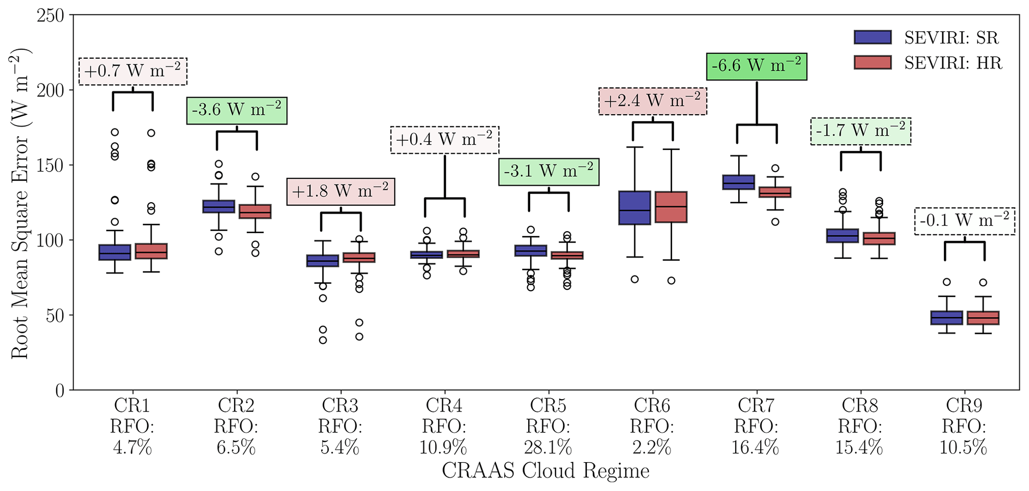
Figure 8 Same as Fig. 5 but separated according to the CRAAS cloud regimes. The relative frequency of occurrence (RFO) for each regime is indicated below the x axis.

The significant improvement for the cirrostratus regime is surprising as we do not expect this regime to be the most spatially and temporally varying. However, inspection of the cloud fields where the cirrostratus cloud regime occurs shows that, in many cases, there are fine-scale fluctuations in GHI that are better resolved at HR. Further inspection using the NWC SAF cloud types shows that, during the field campaign, the cirrostratus cloud regime consists of semi-transparent clouds above medium- or low-level clouds for about 20 % of the time (not shown), explaining the visually observed increased variability for this regime.

For the clear-sky regime, no significant differences are found between both resolutions. Since this regime only consists of data selected from the 10 most clear-sky days identified by the VI method, the boxplots are identical to those shown in Fig. 5a for a 5 min averaging period. A small deterioration in accuracy is observed for the remaining four cloud regimes when the downscaling algorithm is applied. Only for the deep-convection cloud (CR3) regime is this difference statistically significant. CR3 consists of the thickest clouds with the highest total cloud fractions. The regime mostly represents convective and storm systems over Europe (Tzallas et al., 2022b). Under these homogeneous conditions, in terms of small-scale cloud variability, we expect no added value of the downscaling algorithm.

The decrease in accuracy for the shallow-cumulus cloud regime (CR6) is remarkable. This regime is expected to consist of the smallest and most variable clouds of the HOPE field campaign both spatially and temporally. Therefore, one might expect an increase in accuracy for this regime when applying the downscaling. It must be noted that the number of observations that fall within this category is very limited since this regime mainly has an oceanic character (Tzallas et al., 2022b). With only 2.2 % of the total number of observations falling within this regime, it is the least populated of the nine defined cloud regimes.

Accurate retrieval of cloud properties becomes increasingly challenging with SEVIRI when there is a high amount of subpixel variability resulting from fine-scaled cloud fields. Even the HR retrieval will then still have too coarse a spatial resolution to fully capture all the complexity that can be observed in many shallow-cumulus cloud fields. Furthermore, using RMSE as a validation metric, in particular the HR retrieval might suffer from double-penalty issues. With very local clouds occurring, the time matching between the SEVIRI retrieval over the Jülich domain and the 5 min averaged observations of the pyranometer network can become uncertain. A smoother retrieval might be less sensitive to these uncertainties.

Comparing the different CRAAS regimes, it becomes apparent that, in general, the observed RMSE is very regime-dependent. The resolution differences are minor compared to the regime differences. CR7 and CR2 show the largest median improvements with values of 6.6 and 3.6 W m⁻² between HR and SR, respectively. Meanwhile, these regimes also have the highest overall RMSE. Comparing the stratocumulus regime (CR7) to the clear-sky days (CR9), the median RMSE for CR9 is almost 100 W m⁻², or a factor of 3, lower.

5 Discussion

In this Discussion section, we elaborate on the following topics. First, in Sect. 5.1, we focus on some of the uncertainties within the pyranometer network. Next, in Sect. 5.2 and 5.3, respectively, the accuracy of the downscaling algorithm as a result of the spatial- and temporal-averaging length scales are discussed. In Sect. 5.4, the focus is on the diurnal cycle of the GHI retrieval. Finally, in Sect. 5.5, we briefly review our method used to account for possible parallax displacement.

5.1 Pyranometer network uncertainties

Consistent throughout the entire duration of the field campaign and also between various cloud conditions is that the GHI retrieved with SEVIRI tends to overestimate what is measured with the pyranometer network (e.g. Fig. 7). As is covered by Madhavan et al. (2016), there are some operational uncertainties for the pyranometer network. One of these uncertainties is related to the soiling of the pyranometers. As it was not feasible to maintain the 99 pyranometer stations continuously for the entire duration of the field campaign, an underestimation of measured GHI might be expected due to soiling, especially during or after slight precipitation events. Further uncertainties are deviations in GHI within the silicon photodiode pyranometers themselves; slight deviations in the horizontal alignment of the pyranometers; and nearby structures that might be interfering with observations, especially at larger solar zenith angles. Considering these issues, a standard uncertainty of ±15 W m⁻² was assumed during the HOPE campaign (Madhavan et al., 2016).

Furthermore, the limited spectral response of the pyranometers should also be considered. The silicon photodiode pyranometers have a spectral response sensitive to wavelengths between 0.3 and 1.1 µm. This means that the pyranometers are sensitive to variations in aerosols and COT but do not have the sensitivity necessary to measure GHI variations due to differential absorption by liquid and ice cloud particles and by particles of different sizes, occurring at wavelengths in the shortwave infrared, outside the range of sensitivity of the pyranometer. In addition, variations in water vapour absorption at these larger wavelengths are not captured.

5.2 Dependence on the spatial-averaging length scale

Our validation study shows that, as expected, accurately retrieving GHI is most challenging for variable conditions. For the variable days, the highest overall RMSE values are found. Meanwhile, the largest improvements in GHI with the HR retrieval are also found for variable conditions. Thus, the beneficial effect of the downscaling algorithm is largest when it is most needed. However, for overcast situations, a slight deterioration in accuracy with respect to the standard GHI retrieval is obtained. In these relatively homogeneous conditions we would expect that most of the spatial variability that can be resolved at HR can also be resolved at SR. However, a decrease in accuracy for overcast conditions at HR is surprising. This decrease can be better understood when the spatial-averaging length scale is considered.

So far, a fixed filter width σ of 1.0 km has been used. When the RMSE of GHI is plotted as a function of σ (Fig. 9), the optimal σ can be determined as the value where RMSE is at its minimum. Over all the dates of the field campaign the optimal filter widths for HR and SR are around 1.7 and 2.2 km, respectively, while the largest HR improvement occurs for σ between 1.0 and 1.5 km (Fig. 9a). Variable days yield slightly lower optimal values of σ (about 1.4 and 1.9 km), and the largest HR improvement is again found for σ just above 1.0 km (Fig. 9b). In contrast, for the overcast days the minimal RMSEs for both HR and SR are achieved when σ approaches 5.0 km, and for smaller filter widths the SR RMSE is smaller than the HR RMSE (Fig. 9c). For clear-sky conditions the dependence of the RMSE on σ is negligible (not shown), which is expected because there is hardly any spatial variability in GHI.

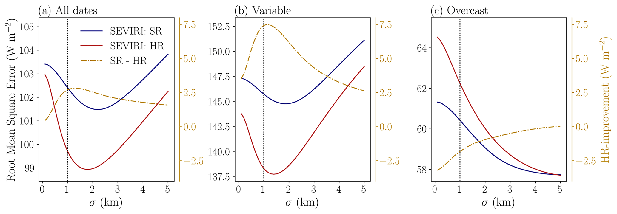
Figure 9 The mean root mean square error at HR (SEVIRI: HR) and SR (SEVIRI: SR) resulting from comparison of SEVIRI-derived and pyranometer-based GHI as a function of the filter width for all conditions (a), variable days (b), and overcast days (c). On the secondary axis, the HR improvement (i.e. the difference in median RMSE between SR and HR) is plotted. The vertical dotted line indicates the filter width of 1 km adopted elsewhere in this study.

We explain the varying dependence of RMSE on filter width for different cloud conditions as follows. The SEVIRI retrievals are spatially averaged to account for their scale mismatch with the pyranometers. Yet, the spatial scale measured by the pyranometers in the network is not constant but rather related to cloud conditions. In fully overcast conditions, the GHI measured by the pyranometers consists solely of diffuse irradiance, which originates from the scattering of radiation by clouds in the wider surroundings. In partially cloudy and clear-sky conditions, the diffuse irradiance fraction is negligible and radiation comes from a smaller region. This is consistent with the results from Fig. 9, which suggest that the pyranometer measurements are representative of an area of at least 5 km for overcast conditions versus 1–2 km for variable conditions.

We can also explain why the SR retrievals have a smaller RMSE than the HR retrievals for filter widths below 5 km in overcast conditions. This is because applying Gaussian filtering to the SR pixels of around 6 km × 3 km yields coverage of a larger area than applying the same filtering to the HR pixels of 2 km × 1 km (irrespective of the filter width), and this larger area is closer to the ∼ 5 km area for which the pyranometer measurements are representative.

5.3 Dependence on the temporal-averaging length scale

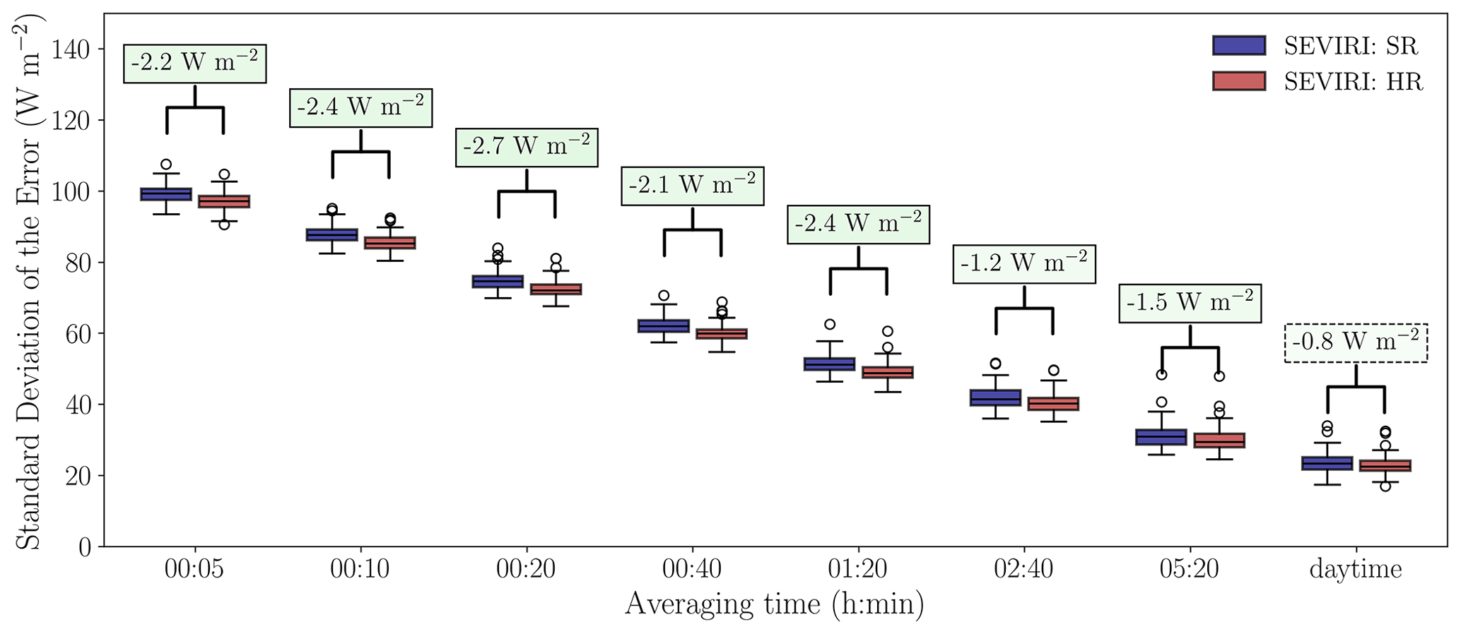
In Fig. 4, a decrease in RMSE is shown when longer averaging timescales are considered. This section studies the relation between the observed error and the temporal-averaging length scale in more detail. Since the bias is independent from the length of the averaging period, it becomes the dominating contribution to the RMSE towards daily timescales. The median HR bias is, over the entire duration of the field campaign, 3.3 W m⁻² smaller than the SR bias, and this would favour the HR product in terms of RMSE for longer averaging times. Therefore, as we are interested in variability rather than systematic offsets, Fig. 10 displays the SDE rather than the RMSE. With this metric, taken over all the dates of the field campaign, the HR gain in accuracy is largest at a 20 min averaging time. This might be explained as follows. Especially for shorter timescales, a spatial mismatch may occur between what is measured by SEVIRI and the pyranometer network. This mismatch may result from deviations between the applied daily mean optimal spatial shift and what would be the actual optimal spatial shift at the selected time step. Since the HR retrieval is more spatially variable than the SR retrieval, the spatial mismatch errors will be larger at HR. By temporal averaging, the spatial variability diminishes. This means on one hand that HR information is lost but on the other hand that the spatial mismatch error becomes a less important factor. The 20 min averaging time could be the optimal trade-off between a good spatial representation with still enough HR information included. Interestingly, earlier work by Huang et al. (2016) recommends using a 30 min temporal-averaging time for routine validation. They argue that at smaller timescales, retrieval accuracy is increasingly affected by representation errors originating from, for instance, 3D radiative effects or cloud inhomogeneities. Our results do show that the most significant HR improvement in SDE occurs at 20 min timescales. However, even at 5 min timescales, additional skill remains included for the HR retrieval. For longer averaging periods, the HR benefit decreases. Surprisingly, the benefit of the HR retrieval remains statistically significant up to an averaging time of approximately 5 h. Moreover, with an improvement of 4.8 %, the relative HR gain is even larger for this averaging period. Only for daytime averages are no significant differences found anymore between HR and SR.

Figure 10 Same as Fig. 5 but showing the standard deviation of the error (SDE). The results are plotted for averaging periods that are doubled from 5 min to daytime averages (from 06:15 to 16:45 UTC).

5.4 Diurnal cycle

Up to this point, the effect of the diurnal cycle of GHI in the validation has not yet been considered. Therefore, in Fig. 11, the RMSE between SEVIRI and the pyranometer network is shown for hourly intervals. The RMSE is normalized with the corresponding mean GHI from the pyranometer network to better compare different time slots.

Figure 11 Same as Fig. 5 but separated according to the time of day in hourly bins.

Overall, the relative RMSE is smallest just before solar noon (10:15–11:10 UTC), with median RMSE values just above 20.0 %. For both resolutions, the relative RMSE increases towards the morning and afternoon. Note that GHI follows a strong diurnal cycle, especially under clear-sky conditions, with fluxes peaking around noon. Therefore, in terms of absolute RMSE, the measurement errors around noon are larger than at other times.

Between 10:15 and 14:10 UTC, we find significant improvements in relative RMSE with relative median reductions between HR and SR ranging from 4.52 % to 7.61 %. In contrast, for the first (06:15–07:10 UTC) and the last two (14:15–15:10 and 15:15–16:10 UTC) hourly periods a significant deterioration in accuracy is obtained when applying the downscaling algorithm. The corresponding median increases of relative RMSE between HR and SR for these three hourly periods are 3.23 %, 2.50 %, and 4.96 %, respectively. No significant differences are found for the remaining time slots between 07:15 and 10:10 UTC. The finding that the most significant improvements in accuracy are observed around noon is relevant to PV applications, since during these hours the GHI potential and corresponding effects on the power grid are largest. It is worth mentioning that the results of Fig. 11 not only show the accuracy of the downscaling algorithm throughout the day but also implicitly reveal the choices made for the mean optimal shift, as is explained next.

5.5 Spatial corrections

In this study, we apply a mean geolocation shift to account for possible inaccuracies and instabilities in the rectification to the SEVIRI grid as well as for parallax and shadow displacements. This method has some uncertainties. For instance, higher clouds require more displacement to account for parallax and shadow effects than low clouds. By using the mean shift for situations with high clouds, the displacement is thus likely underestimated.

Another limitation of using a daily averaged mean optimal shift is that diurnal variations in the optimal displacement are averaged out. While the parallax correction is independent of solar position, this does not hold for the correction to the cloud shadow location, which depends on solar azimuth and zenith angles. Using the collocation shift method, implicitly, a correction for both parallax displacement and shadow position is performed. Therefore, the diurnal cycle of the cloud shadow location is reflected in the displacement of the mean optimal shift. This is a source of errors, especially earlier in the morning and later in the afternoon, since the actual optimal shift will deviate the most from the daily averaged mean optimal shift.

Another limitation of using the mean optimal shift to correct for parallax displacements is that the method is not feasible for most (operational) applications. The method of the mean optimal shift requires ground truth from a pyranometer station to perform the collocation shift, which in many cases will not be available. However, for validating the downscaling algorithm, the method of the mean optimal shift is suitable as ground-based observations are available. Especially around noon, the results from the collocation shift method could be seen as the maximum improvement that can be achieved from using HR instead of SR.

For an operational implementation, parallax correction can be implemented by deriving the cloud top height (CTH) and using this together with the satellite position to calculate the spatial displacement (e.g. Beyer et al., 1996; Vicente et al., 2002; Bieliński, 2020). Similarly, corrections can be made for the effect of cloud shadows on the earth's surface (Roy et al., 2023). While implementing these geometric correction themselves is straightforward, it is often more complicated in practice. One of the complicating factors, for instance, is that there are multiple ways to handle the CTH retrieval (Lorenzo et al., 2017; Miller et al., 2018; Roy et al., 2023). Furthermore, for an accurate geometric correction, the vertical distribution of the cloud field is highly relevant. Solely relying on CTH data might only partially account for the effect of clouds on GHI retrieved at the surface. A study on how to best apply parallax and shadow corrections is outside the scope of this paper and will be part of future work.

6 Conclusions and outlook

In the present paper, we validate a GHI retrieval with improved spatial resolution from Meteosat SEVIRI based on a downscaling algorithm. This downscaling algorithm relies on a combination of reflectances from the high-resolution visible and standard-resolution channels of SEVIRI to obtain cloud physical properties and GHI at an increased resolution. Validation is performed against a dense network of 99 pyranometers spread out over an area of 10 km × 12 km from 18 April to 22 July 2013 in Jülich, Germany, during the HOPE field campaign. We demonstrate that retrieving GHI at an increased spatial resolution of 1 km × 1 km at nadir instead of the standard 3 km × 3 km leads to significant improvements in accuracy, especially for variable cloud conditions.

Over the entire field campaign period, we find a small but statistically significant improvement in accuracy of 2.8 W m⁻² when the HR retrieval is used instead of the SR retrieval. This result is valid for the original 5 min time resolution of the satellite observations but interestingly persists even when aggregated to longer periods up to approximately 5 h. For 60 out of 96 d, the RMSE of the HR retrieval is smaller than the SR retrieval. The largest improvements in GHI accuracy occur on the days when GHI fluctuates strongly. For the 10 most variable days, a median reduction in RMSE of 7.9 W m⁻² is found when the downscaled product is used. We do not find significant differences in accuracy between both resolutions on clear-sky and fully overcast days. For fully overcast conditions, it is suggested that the pyranometer measurements are representative of scales of at least 5 km, which explains why the downscaling algorithm does not provide improved agreement.

When the downscaling algorithm is validated for individual cloud regimes as identified by the CRAAS cloud regime dataset, the largest improvement in accuracy occurs for the stratocumulus regime, with a median RMSE reduction of 6.6 W m⁻² between standard and high resolution. For cirrostratus and mid-level clouds, we also find a significant improvement in accuracy when the downscaling is applied. Together, these three cloud regimes make up 51 % of all field campaign observations. Only for the deep-convection cloud regime is a statistically significant deterioration in accuracy for the high-resolution retrieval found. For the other cloud regimes, no significant differences in accuracy are observed between the two resolutions.

These considerations also demonstrate the benefits of conducting a cloud-regime-based validation of GHI. The large inter-regime differences in validation statistics imply that the overall accuracy is strongly influenced by the frequency of occurrence of individual cloud regimes. Knowledge of the cloud regime can inform one about the expected accuracy of the retrieval, as well as the variability of GHI. To our knowledge, this study is the first to conduct such a regime-based validation approach, but we hope to see wider adoption in the future. The question of how to optimally define and classify the cloud regimes remains open here.

Overall, this study demonstrates that an increased spatial resolution of satellite measurements yields more accurate GHI retrievals, which is important for scientific applications as well as for the practical use of the data. The downscaling approach applied in this study can be transferred to other satellite instruments, such as the Advanced Baseline Imager (ABI) on the third-generation Geostationary Operational Environmental Satellites (GOES), by combining its 0.6 µm channel at 0.5 km × 0.5 km with coarser-resolution channels. The added value of this 2-fold higher spatial resolution remains to be proven since satellite retrievals may become increasingly affected by horizontal photon transport between neighbouring pixels, which effectively smoothens the information content. Similar to GOES ABI, the Flexible Combined Imager (FCI) on board Meteosat Third Generation (MTG) satellites will allow for retrieving cloud physical properties and GHI at a resolution down to 0.5 km × 0.5 km.

In addition, with the SEVIRI downscaling algorithm, the resolution gap between the second- and third-generation Meteosat satellites can be bridged for cloud physical properties and GHI, enabling longer-term climate data records at 1 km × 1 km resolution consisting of both MSG and MTG observations. While the results presented here demonstrate the potential of the downscaling, further research should focus on the validation of the cloud properties and ensuring the homogeneity of such a combined data record.

With the increase in spatial resolution, it also becomes increasingly important to ensure that the geolocation of the satellite products remains accurate. For this validation study, accurate geolocation was achieved by deriving an optimal mean spatial collocation shift with reference to the pyranometer observations. However, this method cannot be applied to regions where or periods when ground-based observations are lacking. In future work, we will use the HOPE field campaign to investigate parallax and shadow correction implementations, enabling a more reliable downscaling for arbitrary regions and periods.

Appendix A: Visual inspection of HOPE pyranometer data

The visual inspection is conducted on a daily basis. The general idea of the visual inspection is that sensors affected by measurement issues can be identified as outliers in space or time. As a first criterion, stations are flagged based on their daily averaged irradiance. By examining both the spatial distribution and the probability density distribution of daily averaged irradiance for many days, we can observe a few clear outliers (Fig. A1). Subsequently, a more detailed visual analysis is conducted by examining the time series of GHI for each of the sensors, confirming that for some of the sensors the GHI measurements are abnormally low (most probably due to a tilt of the pyranometer). Furthermore, for some of the sensors, the time series representation also reveals sudden drops in GHI to abnormally low values (almost zero during the day). Even if, for the latter case, the measured values lie within the ERL range, we consider this behaviour suspicious and manually flag the sensor. After quality control, the number of valid stations varies between 70 and 90 for each time step (Fig. A2).

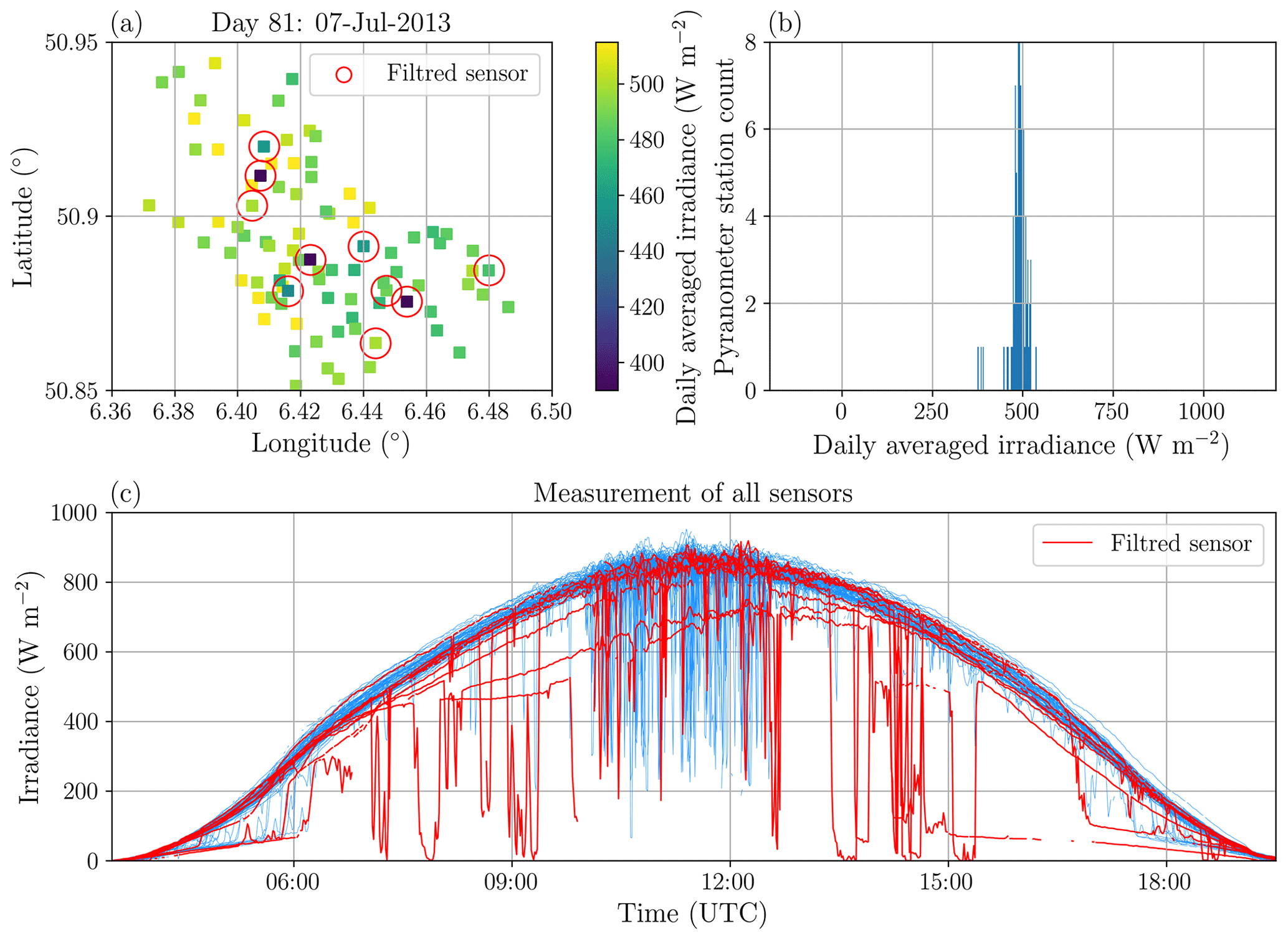
Figure A1 Plots used for the visual control of the HOPE measurements. Panel (a) represents the daily average of the measurements of each sensor; panel (b) is the distribution of the daily measurements. In panel (c), the time series for each of the sensors is represented. Flagged measurements are marked in red.

For each day, all sensors exhibiting abnormal behaviour, as discussed above, have been listed. A conservative flagging strategy is employed to ensure that as few faulty measurements as possible are used for the validation. When an issue is suspected during the visual inspection, a sensor is flagged for the entire day (Fig. A3).

Figure A2 Number of valid measurements as a function of time before (blue line) and after (red line) quality control.

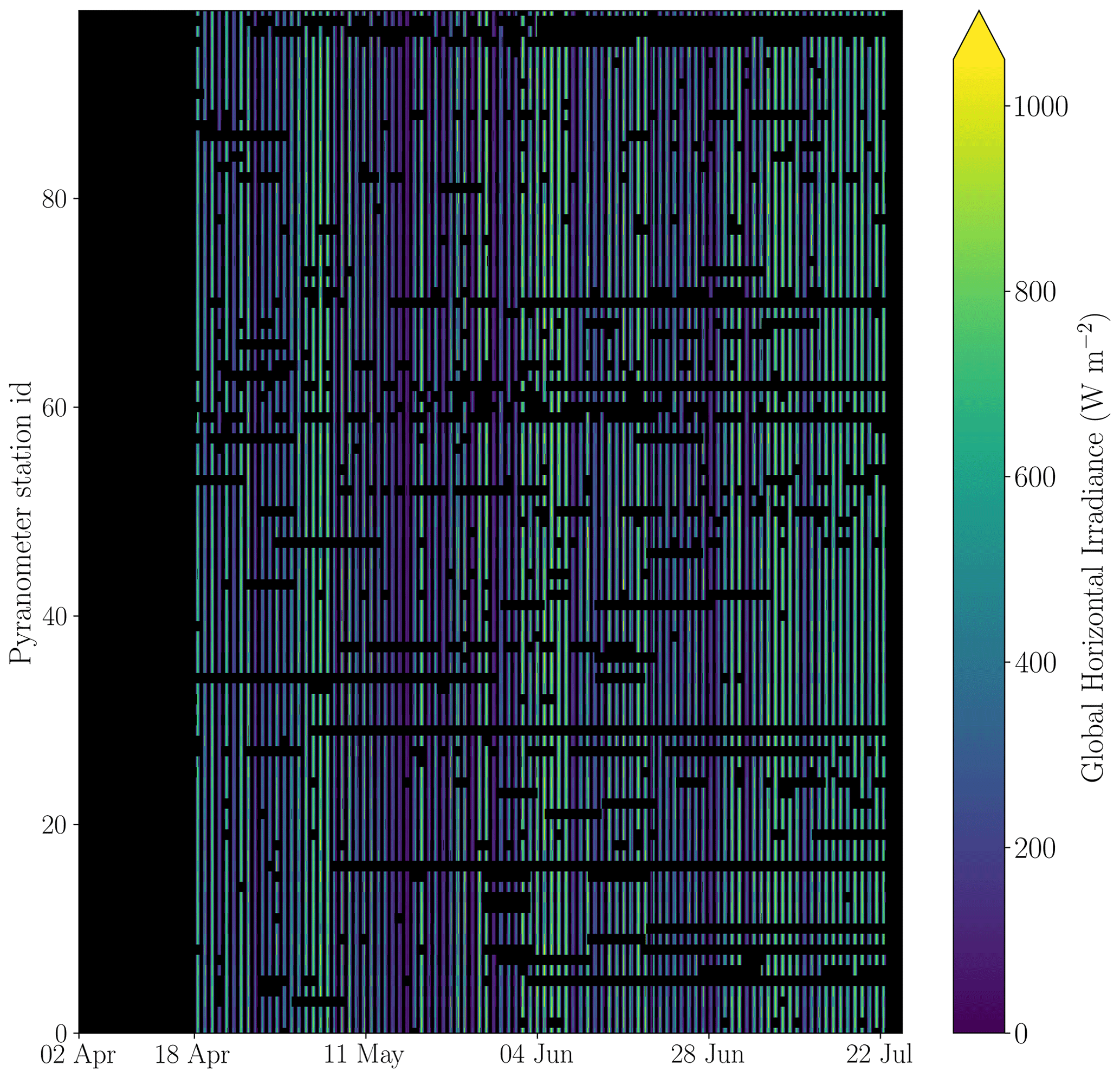
Figure A3 Global horizontal irradiance for each of the 99 pyranometer stations as a function of time during the HOPE field campaign. Invalid data are illustrated by the black boxes.