Lower-cost eddy covariance for CO₂ and H₂O fluxes over grassland and agroforestry

Eddy covariance (EC) measurements can provide direct and non-invasive ecosystem measurements of the exchange of energy, water (H₂O) and carbon dioxide (CO₂). However, conventional eddy covariance (CON-EC) setups (ultrasonic anemometer and infrared gas analyser) can be expensive, which recently led to the development of lower-cost eddy covariance (LC-EC) setups (University of Exeter). In the current study, we tested the performance of an LC-EC setup for CO₂ and H₂O flux measurements at an agroforestry and adjacent grassland site in a temperate ecosystem in northern Germany. The closed-path LC-EC setup was compared with a CON-EC setup using an enclosed-path gas analyser (LI-7200, LI-COR Inc., Lincoln, NE, USA). The LC-EC CO₂ fluxes were lower compared to CON-EC by 4 %–7 % (R²=0.91–0.95), and the latent heat (LE) fluxes were higher by 1 %–5 % in 2020 and 23 % in 2021 (R²=0.84–0.91). The large difference between latent heat fluxes in 2021 seemed to be a consequence of the lower LE fluxes measured by the CON-EC. Due to the slower response sensors of the LC-EC setup, the (co)spectra of the LC-EC were more attenuated in the high-frequency range compared to the CON-EC. The stronger attenuation of the LC-EC led to larger cumulative differences between spectral methods of 0.15 %–38.8 % compared to 0.02 %–11.36 % of the CON-EC. At the agroforestry site where the flux tower was taller compared to the grassland, the attenuation was lower because the cospectrum peak and energy-containing eddies shift to lower frequencies which the LC-EC can measure. It was shown with the LC-EC and CON-EC systems that the agroforestry site had a 105.6 g C m⁻² higher carbon uptake compared to the grassland site and 3.1–14.4 mm higher evapotranspiration when simultaneously measured for 1 month. Our results show that LC-EC has the potential to measure EC fluxes at a grassland and agroforestry system at approximately 25 % of the cost of a CON-EC system.

1 Introduction

Reducing carbon dioxide (CO₂) and other greenhouse gas (GHG) emissions can minimize the effects of global warming and climate change (Griscom et al., 2017; Anderson et al., 2019; IPCC, 2021). In addition, mitigating CO₂ emissions with nature-based climate (management) solutions (NbCSs) is seen as a fairly rapid and low-cost solution, which simultaneously can provide environmental co-benefits (Griscom et al., 2017; Anderson et al., 2019). Agroforestry is an example of an NbCS, which can contribute to resilient agriculture adapted for climate change by providing a more favourable local microclimate (Schoeneberger et al., 2012; Smith et al., 2013; Cardinael et al., 2021), increased biodiversity (Jose, 2009; Torralba et al., 2016) and a reduction in soil erosion (Schoeneberger et al., 2012; van Ramshorst et al., 2022). Nevertheless, robustly validating estimations and models of the carbon sequestration potential of NbCSs is not straightforward and is time- and labour-intensive (Griscom et al., 2017; Novick et al., 2022). Direct observations with eddy covariance (EC) can provide solid and independent measurements to validate the carbon uptake of the entire ecosystem (Hemes et al., 2021; Novick et al., 2022; Wiesner et al., 2022).

Eddy covariance is a non-invasive technique to directly measure the net land–atmosphere exchange (flux) of energy, water (H₂O), CO₂ and other GHGs over an area of up to several hectares (Baldocchi, 2003; Lee et al., 2005; Baldocchi, 2008). Currently, several global networks of EC towers provide essential data quantifying the net carbon exchange (Sabbatini et al., 2018; Pastorello et al., 2020; Heiskanen et al., 2022) and associated climate and land use change impacts for a variety of ecosystems. However, conventional EC (CON-EC) systems are expensive, and therefore the number of observations is often limited to primary ecosystems and users who can afford EC (Schimel et al., 2015; Hill et al., 2017; Baldocchi, 2020). Consequently, a small number of EC towers are generally used to represent an ecosystem, which could raise concerns regarding the spatial representativeness of flux measurements, especially when the ecosystem is heterogeneous (Hill et al., 2017; Cunliffe et al., 2022).

Recently, several lower-cost eddy covariance (LC-EC) gas analysers have been developed to provide cheaper but still accurate and robust measurements of H₂O fluxes (Markwitz and Siebicke, 2019) and a combination of CO₂ and H₂O fluxes (Hill et al., 2017; Cunliffe et al., 2022). These LC-EC systems use more economical parts and have slower-response sensors, which lead to a price reduction compared to CON-EC. The LC-EC system of the current study has a price reduction of approximately 75 % compared to CON-EC (Cunliffe et al., 2022). Using slower-response sensors, however, leads to an increased loss of high-frequency signal, and accordingly this leads to an increased measurement uncertainty (Hill et al., 2017; Markwitz and Siebicke, 2019; Cunliffe et al., 2022). Nevertheless, previous field comparison of LC-EC systems provided flux measurements in agreement with a CON-EC setup (Hill et al., 2017; Markwitz and Siebicke, 2019; Cunliffe et al., 2022).

Spectral corrections are inevitable with the EC methodology (Massman and Clement, 2005; Emad, 2023). The additional loss of high-frequency signal of LC-EC setups increases the importance of these applied corrections (Mauder and Foken, 2006; Reitz et al., 2022). Generally, the magnitude of spectral losses depends on, for example, the response time of sensors and the EC system as a whole (Leuning and Moncrieff, 1990; Massman and Lee, 2002; Polonik et al., 2019), the measurement height of the EC tower (Moncrieff et al., 1997; Reitz et al., 2022), the length and diameter of the tubing when present (Leuning and Moncrieff, 1990; Massman, 1991), the flow rate and flow regime inside the tube (Leuning and Moncrieff, 1990; Massman, 1991), and the absorption and desorption of water molecules inside the tubing (Massman, 1991; Ibrom et al., 2007; Polonik et al., 2019). Furthermore, there are many different spectral correction methods available, each with their own assumptions and uncertainties (Polonik et al., 2019; Reitz et al., 2022; Emad, 2023).

In the current study we tested LC-EC setups over a temperate grassland and an adjacent alley cropping agroforestry grassland near Hanover in Germany. Due to the LC-EC setup's larger loss of high-frequency signal, it is expected that the spectral corrections will be higher and more varied compared to the CON-EC. In order to identify potential reasons for the difference between the two EC setups, the objectives of this paper are to (i) perform a technical characterization of the LC-EC setup relative to CON-EC in a temperate ecosystem setting, (ii) investigate the effect of the spectral correction method applied, and (iii) present the first application of LC-EC over a grassland and alley cropping agroforestry grassland.

2 Methods

2.1 Site characterization

The current study took place at a grassland site in Mariensee, Lower Saxony, Germany ($\mathrm{52}\mathit{°}{\mathrm{33}}^{\prime }{\mathrm{52.3}}^{\prime \prime }$ N, $\mathrm{9}\mathit{°}{\mathrm{27}}^{\prime }{\mathrm{51.2}}^{\prime \prime }$ E) (Fig. 1). The 7 ha grassland site includes three parallel north- and south-orientated willow tree strips of approximately 6.5 m height during the time of the study (Markwitz et al., 2020). Mowing of the non-grazed grassland was done twice a year, once in summer and once in autumn. The soil consists of Histosol and Anthrosol and has a bulk density of 1.28 kg m⁻³ (Beule et al., 2019; Markwitz et al., 2020).

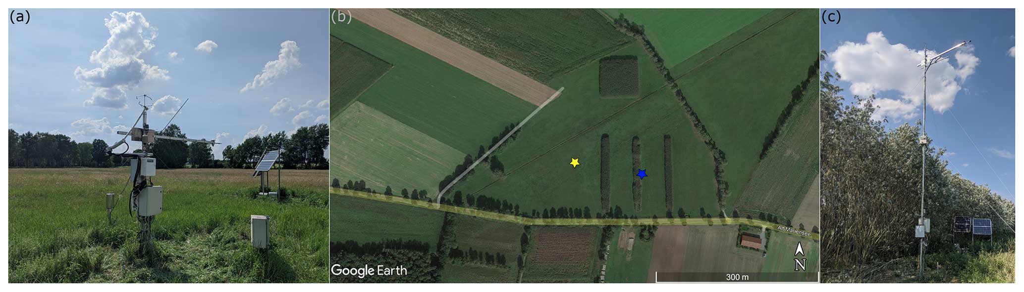
Figure 1 (a) The Mariensee grassland tower west of the tree strips in June 2020. The photo faces west (photo by Justus G. V. van Ramshorst). (b) Satellite image from the Mariensee site, with the yellow and blue star indicating the location of the grassland tower and the agroforestry tower, respectively (© Google Earth 2022). (c) The Mariensee agroforestry tower east of the central tree strip in August 2020. The photo faces north-west (photo by Justus G. V. van Ramshorst).

The long-term (1981–2010) average annual sum of precipitation is 662 mm, and the average annual mean temperature is 9.6 °C according to the Hanover weather station of the German Meteorological Service (station ID: 2014). Based on gap-filled meteorological data of our own grassland site in Mariensee, in 2020 and 2021 the annual precipitation was 521 and 597 mm, and the annual mean temperature was 11.3 and 9.8 °C, respectively. The long-term mean wind speed at 3.0 m height was 1.87 m s⁻¹, and the dominant wind directions at the site were west and south-west, based on gap-filled meteorological data of Mariensee from 2019–2021.

The site was part of the Sustainable Intensification of Agriculture through Agroforestry (SIGNAL) project, which investigates under which site conditions agroforestry can be a sustainable solution for future agriculture (Veldkamp et al., 2023). As part of the SIGNAL project, two EC towers were installed to measure and compare the micro-climate and CO₂ sequestration and evapotranspiration (ET) of the agroforestry grassland and the conventional grassland (Fig. 1).

2.2 Instrumental setup

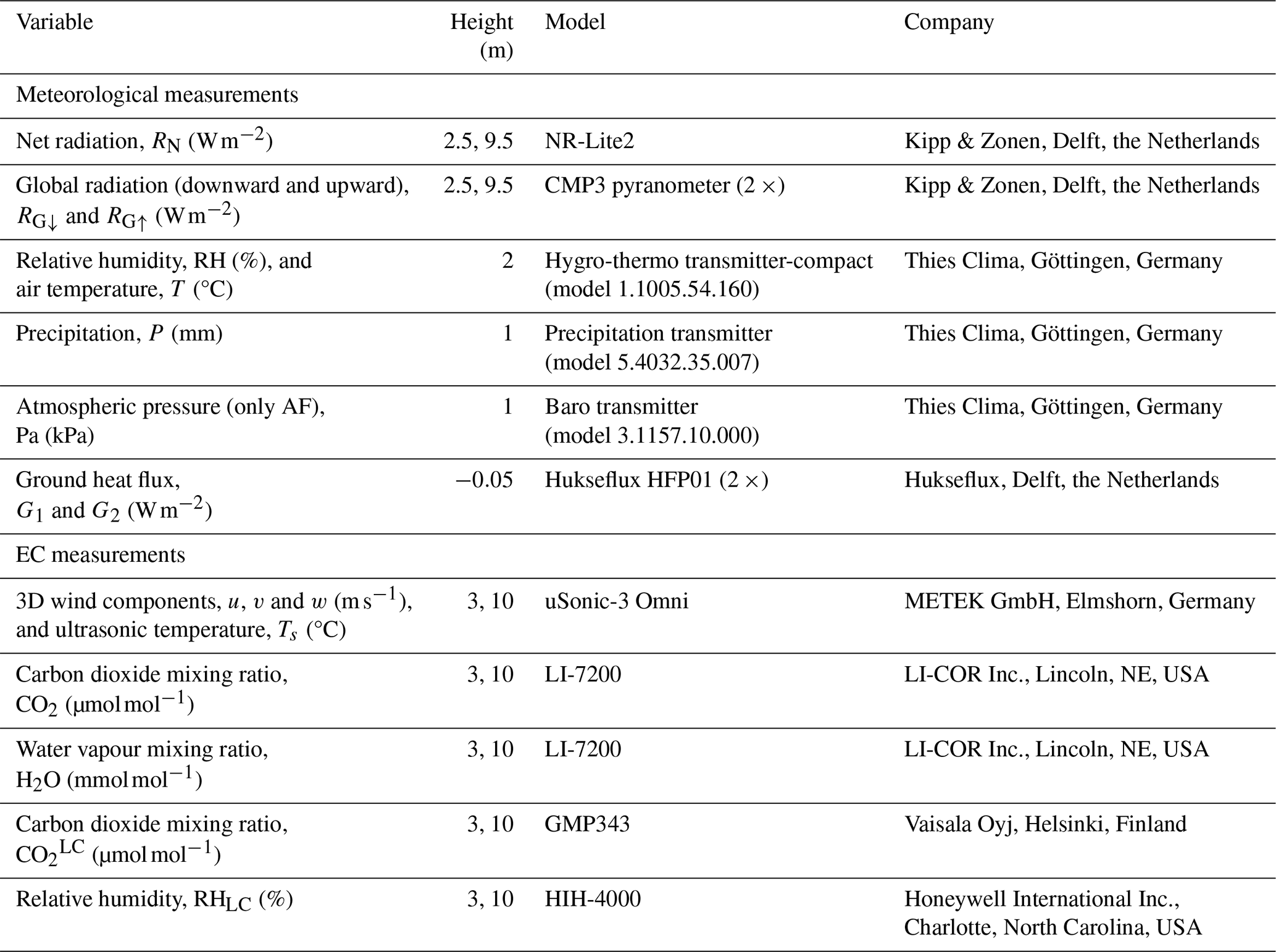
The grassland EC tower was 3 m in height and placed west of the tree strips. The agroforestry EC tower was 10 m tall and placed next to the central tree strip. Both EC towers in Mariensee were equipped with similar instrumentation for meteorological measurements and EC (Table 1). Meteorological data were measured every 10 s and logged on a CR1000X data logger (Campbell Scientific, Inc., Logan, Utah, USA). The EC data, including an ultrasonic anemometer, were measured at 2 Hz (LC-EC and CON-EC in 2020) and 20 Hz (CON-EC in 2021) frequency and logged on a CR6 data logger (Campbell Scientific, Inc., Logan, Utah, USA).

Table 1 Meteorological and eddy covariance instruments, with height, model and company installed at both EC towers. All meteorological sensors were sampled every 10 s, except for precipitation, which is the cumulative sum over 10 s. All EC sensors were sampled at either 2 Hz or 20 Hz.

2.2.1 Lower-cost eddy covariance

The LC-EC setups were present from the summer of 2019 until January 2022; however in the current study only data measured during the EC measurement campaigns in 2020 and 2021 were used for comparison. The LC-EC setup in the current study was very similar to that used by Cunliffe et al. (2022) and was custom-built at the Department of Geography at the University of Exeter, UK. The LC-EC uses a uSonic-3 Omni 3D ultrasonic anemometer (METEK GmbH, Elmshorn, Germany) and a closed-path gas analyser enclosure. Inside the custom-made enclosure, the CO₂ mole fraction (${{\mathrm{CO}}_{\mathrm{2}}}^{\mathrm{LC}}$) was measured with a GMP343 infrared gas analyser (IRGA) (Vaisala Oyj, Helsinki, Finland), and inside the same cell the relative humidity (RH_LC) was measured with an HIH-4000 RH sensor (Honeywell International Inc., Charlotte, North Carolina, USA). The sensor response times of the GMP343 and HIH-4000 are 1.36 and 4 s, respectively (Hill et al., 2017). The accuracy of the GMP343 is $\pm \mathrm{5}\mathrm{\mu }{\mathrm{mol}}_{{\mathrm{CO}}_{\mathrm{2}}}{\mathrm{mol}}_{\text{dry air}}^{-\mathrm{1}}+\mathrm{2}$ % of reading and that of the HIH-4000 is ±3.5 %. The cell temperature ($T_{\text{CELL}}^{\text{LC}}$) was measured using a fine-wire thermocouple (Omega Engineering Inc., Norwalk, Connecticut, USA) with a 0.2 s response time and ±1.8 K accuracy. The absolute cell pressure ($P_{\text{CELL}}^{\text{LC}}$) was measured using an MPX5100AP pressure sensor (NXP USA Inc., Austin, Texas, USA), with a ±1.5 kPa accuracy and 1 ms time response. The enclosure consists of a heater, which can reduce the relative humidity inside the measuring cell during humid conditions to prevent condensation. The vertical separation between the centre of the ultrasonic anemometer and the intake of the sampling tube was −0.2 m, and the east- and northward separation was 0 m. By placing the intake at the bottom of the ultrasonic anemometer, the wind measurements are less disturbed; however small flux losses of 0.71 % for the grassland tower and 0.2 % for the agroforestry tower are expected based on calculations due to sensor displacement (Kristensen et al., 1997). The Synflex 1300 tube (1300-M0603, Eaton Corporation, Dublin, Ireland) had a length of either 2 m (grassland) or 9 m (agroforestry) and an internal diameter of 4.0 mm and was fitted with two stainless steel 2 µm filters (SS-4FW-2, Swagelok, Solon, Ohio, USA). A nominal flow rate of ∼2 L min⁻¹ was achieved with an NMP830KNDC-B diaphragm gas pump (KNF Neuberger Inc., Trenton, New Jersey, USA). The flow rate could drop down to ∼1 L min⁻¹ when highly clogged. The flow rate resulted in a laminar flow with a Reynolds number of 717–358 inside the tubing (Massman, 1991).

2.2.2 Conventional eddy covariance

During three measurement campaigns in 2020 and 2021, CON-EC setups were installed and added to the existing LC-EC towers. In 2020 the CON-EC was effectively sampled at 2 Hz due to a logging issue, and in 2021 the CON-EC was sampled at 20 Hz. The first campaign was at the grassland from 3 June until 25 October 2020, the second at the agroforestry grassland from 20 August until 26 September 2020 and the third at the grassland from 21 July until 26 October 2021. The CON-EC setup shared the same uSonic-3 Omni 3D ultrasonic anemometer (METEK GmbH, Elmshorn, Germany) as the LC-EC. The CO₂ (µmol mol⁻¹) and H₂O (mmol mol⁻¹) mixing ratios were measured using a LI-7200 enclosed-path infrared gas analyser (IRGA) (LI-COR Inc., Lincoln, NE, USA). The sensor response time of the LI-7200 for H₂O was approximately 0.6 ± 0.3 s (Markwitz and Siebicke, 2019) and 0.16 s for CO₂. The vertical separation between the centre of the ultrasonic anemometer and the intake of the sampling tube was −0.2 m, and the east- and northward separation was 0 m. The effect of vertical sensor separation was accounted for as described in Sect. 2.2.1 (Kristensen et al., 1997). The insulated – but not heated – intake tube had a length of 1 m and an inner diameter of 8.2 mm. The flow rate was set at 15 L min⁻¹, which results in a turbulent flow with a Reynolds number of 2623 inside the tubing (Leuning and King, 1992).

2.3 Flux processing

2.3.1 Lower-cost eddy covariance

Pre-processing

The LC-EC method requires some pre-processing steps before the eddy covariance calculations can be applied:

1. The LC cell pressure was smoothed using a 5 min centred moving average window in order to prevent additional noise being added to the covariance calculations.

2. ${{\mathrm{H}}_{\mathrm{2}}\mathrm{O}}^{\text{LC}}$ (mmol mol⁻¹) was calculated from the measured RH_LC, $T_{\text{CELL}}^{\text{LC}}$ and $P_{\text{CELL}}^{\text{LC}}$, following Markwitz and Siebicke (2019).

3. The mixing ratio ${{\mathrm{H}}_{\mathrm{2}}\mathrm{O}}_{\text{DRY}}^{\text{LC}}$ (mmol mol⁻¹) was calculated following Burba et al. (2012).

4. The measured raw ${{\mathrm{CO}}_{\mathrm{2}}}^{\mathrm{LC}}$ (µmol mol⁻¹, LC-EC uncor.) mole fraction needed to be corrected for a variable cell temperature, relative humidity and pressure. This was not done automatically; only a variable cell temperature was used, and constant values of pressure and relative humidity were assumed (LC-EC auto). The final mixing ratio ${{\mathrm{CO}}_{\mathrm{2}}}_{\text{DRY}}^{\text{LC}}$ (µmol mol⁻¹, LC-EC final) was calculated following the iterative equations provided by Vaisala (2023). The CO₂ correction required simultaneously measured RH_LC, $T_{\text{CELL}}^{\text{LC}}$ and $P_{\text{CELL}}^{\text{LC}}$ and several sensor-specific temperature constants, which could be pulled from each individual sensor memory. The effect of this correction is discussed more elaborately in Sect. 2.3.3.

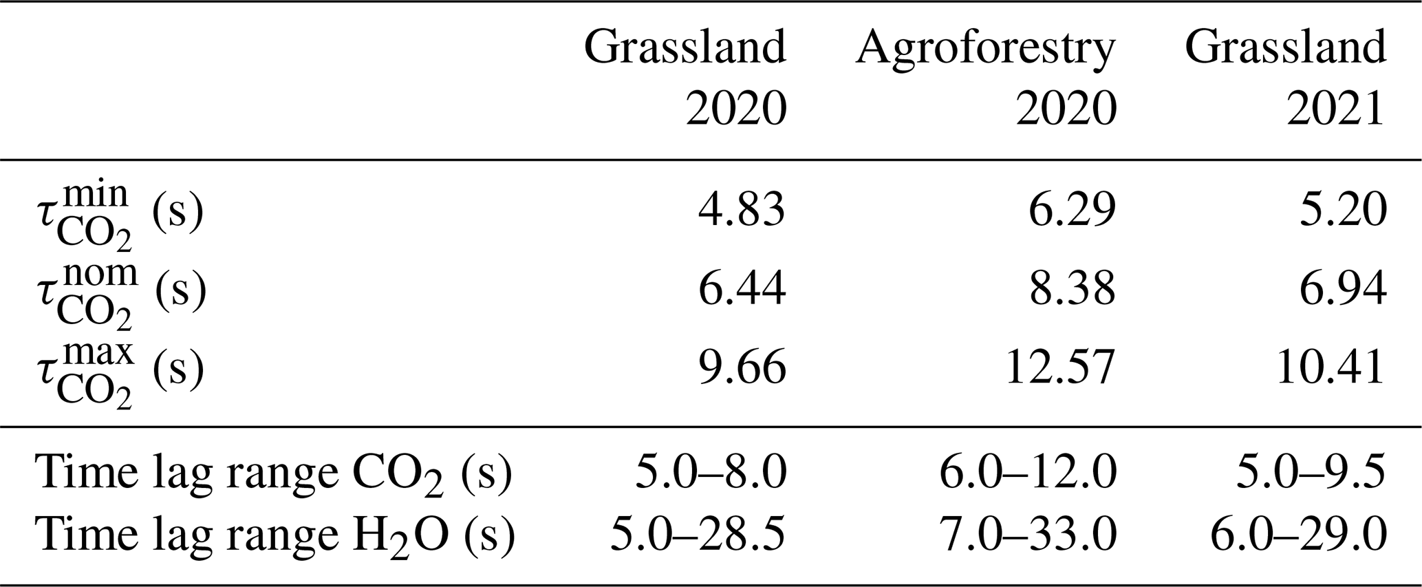
5. The time lags of the LC-EC systems in the current study were considerably larger and more variable compared to a CON-EC setup with a LI-7200 due to the longer tubing in combination with a lower flow rate. This led to unsatisfactory time lag optimization when the standard time lag estimation method in EddyPro was applied. Therefore, realistic time lag windows for CO₂ and H₂O were pre-estimated as follows in order to obtain an accurate time lag optimization in EddyPro. Based on the absolute maximum cross-correlation between the vertical wind speed (w) and ${{\mathrm{CO}}_{\mathrm{2}}}_{\text{DRY}}^{\text{LC}}$, the time lag for CO₂ was estimated for each 30 min data set. The nominal time lag (τ^nom) for each measurement campaign was estimated by determining the density peak of all 30 min time lags. The minimum (τ^min) and maximum (τ^max) time lag for each data set was calculated by multiplying the nominal time lag by 0.75 and 1.5, respectively (Table 2). The time lag window for ${{\mathrm{H}}_{\mathrm{2}}\mathrm{O}}_{\text{DRY}}^{\text{LC}}$ was determined differently, as the time lag of H₂O was more variable due to the effect of absorption and desorption of water. Nevertheless, it was expected that the time lag of H₂O was at least equal to or longer than the time lag of CO₂. In order to avoid a window that is too narrow for the time lag optimization in EddyPro, ${\mathit{\tau }}_{{\mathrm{H}}_{\mathrm{2}}\mathrm{O}}^{\text{max}}$ was fixed at 40 s for all three campaigns, and ${\mathit{\tau }}_{{\mathrm{H}}_{\mathrm{2}}\mathrm{O}}^{\text{min}}$ was assumed to be equal to ${\mathit{\tau }}_{{\mathrm{CO}}_{\mathrm{2}}}^{\text{min}}$. In Table 2, the estimated time lag ranges for quality-controlled CO₂ and H₂O fluxes calculated by EddyPro are shown for the adapted time lag estimation.

Table 2 Estimated time lag windows for CO₂ during each measurement campaign and time lag ranges for quality-controlled CO₂ and H₂O fluxes calculated by EddyPro.

Processing

The LC-EC fluxes based on GMP343 and HIH-4000 were calculated using EddyPro (version 7.0.3). ${{\mathrm{CO}}_{\mathrm{2}}}_{\text{DRY}}^{\text{LC}}$ and ${{\mathrm{H}}_{\mathrm{2}}\mathrm{O}}_{\text{DRY}}^{\text{LC}}$ were pre-calculated, as described in pre-processing steps 2, 3 and 4 in Sect. 2.3.1. Moreover, meteorological data (air temperature, atmospheric pressure, relative humidity and global radiation) measured at the Mariensee stations were provided to EddyPro. During flux processing, double rotation, block averaging and automatic time lag optimization with predefined windows, as shown in pre-processing step 5 in Sect. 2.3.1, were applied. The availability of mixing ratios made additional density (WPL) corrections redundant. Statistical tests for raw data screening were performed following Vickers and Mahrt (1997), and the random uncertainty estimation due to sampling errors was calculated following Mann and Lenschow (1994). Corrections for spectral attenuation in the low-frequency range were performed following Moncrieff et al. (2004). High-frequency spectral attenuations were corrected following two methods, of which the Horst (1997) correction was the main correction used in the current study. Due to noisy spectra in the high-frequency range (see Sect. 3.2.4), the transfer function for the high-frequency correction was fitted from 10⁻⁴ to 0.25 Hz. Additionally, spectral corrections following Ibrom et al. (2007), including Horst and Lenschow (2009) for sensor separation, were applied to investigate the sensitivity of the spectral correction method applied. The method of Horst (1997) is an analytical method, which uses a simple equation to estimate the spectral attenuation of each individual CO₂ and H₂O measurement. The method of Ibrom et al. (2007) is an empirical method that is specifically designed for the attenuation of the strongly RH-dependent H₂O measurements in closed-path EC systems. This method defines the spectral attenuation on a large number of spectra based on RH classes.

2.3.2 Conventional eddy covariance

The EC fluxes from the CON-EC setup were calculated using EddyPro (version 7.0.3), and the applied flux processing was kept as similar as possible to the method applied for the LC-EC in order to prevent additional uncertainties. The LI-7200 provides T_CELL and P_CELL measurements and instantaneous mixing ratios of CO₂ (${{\mathrm{CO}}_{\mathrm{2}}}_{\text{DRY}}$ (µmol mol⁻¹)) and H₂O (${{\mathrm{H}}_{\mathrm{2}}\mathrm{O}}_{\text{DRY}}$ (mmol mol⁻¹)), following Burba et al. (2012). The same meteorological data as for the LC-EC were provided to EddyPro. During flux processing, double rotation, block averaging and automatic time lag optimization (without predefined windows) were applied. Similar to the LC-EC calculations, the availability of dry mixing ratios made additional density (WPL) corrections redundant. Statistical tests for raw data screening were performed following Vickers and Mahrt (1997), and the random uncertainty estimation due to sampling errors was calculated following Mann and Lenschow (1994). Corrections for spectral attenuation in the low-frequency range were performed following Moncrieff et al. (2004). High-frequency spectral attenuations were corrected following two methods, of which the Horst (1997) correction was the main correction used in the current study. Additionally, spectral corrections following Ibrom et al. (2007), including Horst and Lenschow (2009) for sensor separation, were applied to investigate the sensitivity of the spectral correction method applied.

2.3.3 Correction of CO₂ concentration

The automatic correction by Vaisala (LC-EC auto), which only considers a variable cell temperature ($T_{\text{CELL}}^{\text{LC}}$) and assumes constant values of pressure and relative humidity, improved the CO₂ mixing ratio compared to the raw CO₂ mole fraction (LC-EC uncor.) (Fig. S1 in the Supplement). Nevertheless, it is clearly visible that when the full correction was applied (LC-EC final), also considering a variable cell pressure ($P_{\text{CELL}}^{\text{LC}}$) and cell relative humidity (RH_LC), the CO₂ mixing ratio was closest to the CO₂ mixing ratio measured by the LI-7200 (CON-EC). The LC-EC auto correction increases the mean CO₂ concentration compared to LC-EC uncor. by 3 %–4 %, and LC-EC final decreases the mean CO₂ concentration compared to LC-EC uncor. by 2 %–3 %. For the agroforestry 2020 and grassland 2021 campaigns, the offset between the LC-EC and EC is relatively constant during the day. For the grassland 2020 campaign, the offset between the LC-EC and EC is not constant and is larger during midday.

2.3.4 Quality control and gap filling

Similar quality control (QC) was applied for the CO₂, latent heat (LE) and sensible heat (H) fluxes from the CON-EC and LC-EC systems. Only the high-quality data (Flag 0) were used in the current study, based on the 0–1–2 flagging system according to Mauder et al. (2013). Fixed u^* filtering was applied to the CO₂ and LE fluxes, similar to Cunliffe et al. (2022). For the grassland site the $u_{\text{threshold}}^{*}$ was set at 0.1 (m s⁻¹), and for the agroforestry site the $u_{\text{threshold}}^{*}$ was set at 0.15 (m s⁻¹). Furthermore, absolute limits for the CO₂, LE and H fluxes were applied, based on manual screening of the data. CO₂ fluxes below −30 and above 30 $\mathrm{\mu }\mathrm{mol}{\mathrm{m}}^{-\mathrm{2}}{\mathrm{s}}^{-\mathrm{1}}$ were discarded. LE and H fluxes below −50 and above 500 W m⁻² were discarded. After applying the combined QC, 57 %, 70 % and 51 % of the EC CO₂ fluxes were removed, and 52 %, 67 % and 51 % of the LC-EC CO₂ fluxes were removed during the grassland 2020, agroforestry 2020 and grassland 2021 campaigns, respectively. For the EC LE fluxes, 59 %, 74 % and 59 % were removed, and 62 %, 77 % and 64 % of the LC-EC LE fluxes were removed during the grassland 2020, agroforestry 2020 and grassland 2021 campaigns, respectively. During nighttime, defined as incoming shortwave radiation <20 W m⁻², more EC data were discarded than during daytime due to unfavourable turbulent conditions (Papale et al., 2006). For the three LC-EC campaigns combined this was also clearly visible, as 42 % of the daytime data and 81 % of the nighttime data were discarded based on the QC conditions.

As the focus of this study was on instrument performance, we did not apply any gap filling when comparing the LC-EC and CON-EC setups so that only measured data were compared. Therefore, Figs. 1–9 and A1 include quality-controlled but non-gap-filled data. As an exception, Fig. 10 uses gap-filled data to illustrate a real-use case of comparing cumulative ecosystem fluxes of an agroforestry and grassland system. For the gap filling high- and moderate-quality data (Flag 0 or 1) were selected (Mauder et al., 2013). Subsequently, the gap filling was done using XGBoost with five predictors: air temperature, vapour pressure deficit (VPD), global radiation, wind speed and wind direction (Vekuri et al., 2023). The gap-filling uncertainty was evaluated by calculating the standard deviation (SD) of the bias distribution between the measured and modelled 30 min fluxes, and it was propagated through the cumulative sum by multiplying 2SD by the squared root of the number of 30 min filled gaps.

2.3.5 Energy balance closure

The energy balance closure (EBC) for each EC system was assessed as an additional indicator for data quality. In the current study we used the energy balance closure as described in Eq. (1), similar to Mauder and Foken (2006) and Reitz et al. (2022).

$$\begin{array}{}\text{(1)}& H+LE=R_{\mathrm{N}}-G\end{array}$$

With similar net radiation (R_N) and ground heat (G) flux for the CON-EC and LC-EC methods, the difference between the setups was caused by the sensible heat (H) flux and latent heat (LE) flux measured by the EC and LC-EC. Hence, even though the same ultrasonic anemometer was used for the EC and LC-EC setups, H was slightly different due to the humidity correction applied, which includes measurements of ET (van Dijk et al., 2004). G was the average of the two heat flux plates present, G₁ and G₂, when both were available. In the current study, soil storage and canopy storage were not measured and, therefore, not included in the energy balance closure. However, these storage terms would be the same for the EC and LC-EC methods.

Additionally, the cumulative energy balance ratio (EBR) was also calculated and defined as the ratio of the total cumulative sum of the turbulent fluxes (H+LE) to the total cumulative sum of the available energy (R_N−G) (Cunliffe et al., 2022).

2.3.6 Statistical methods

Linear regressions were calculated by applying a major-axis regression with the R package lmodel2 (Legendre and Oksanen, 2018), and the normality of the residuals was checked using Shapiro–Wilk normality tests with the R package stats. The root mean square errors (RMSEs) were calculated using the R package Metrics (Hammer et al., 2018). The significance t tests were calculated using the R package stats.

3 Results

3.1 Meteorological conditions

In 2020, the annual mean air temperature was 1.7 °C above the long-term average of 9.6 °C, and the annual sum of precipitation was 21 % below the long-term average of 662 mm. In 2021, the annual mean air temperature was 0.2 °C above the long-term average, and the annual sum of precipitation was 10 % below the long-term average. During the measurement campaigns, the mean RH and VPD were 78.6 % and 450 Pa and 83.8 % and 299 Pa in 2020 and 2021, respectively. These results show that the campaign in 2020 was held during warmer and drier conditions compared to the campaign in 2021 (Fig. 2). Additionally, the mean Bowen ratio during both campaigns also indicates that the conditions during the campaign in 2020 were less water abundant compared to 2021, as the mean Bowen ratio was 0.35 and 0.24 in 2020 and 2021, respectively. Furthermore, during the measurement campaign in 2020 it was less windy compared to the campaign in 2021, with mean wind speeds of 1.38 and 1.54 m s⁻¹, respectively. Additionally, during the campaign in 2020 it was more sunny compared to the campaign in 2021, as the mean incoming global radiation per day was 14.6 and 11.6 MJ m⁻², respectively. Finally, the average friction velocity, $\stackrel{\mathrm{‾}}{u^{*}}$, was higher during the agroforestry campaign compared to the grassland campaign in 2020, being 0.33 versus 0.20 m s⁻¹.

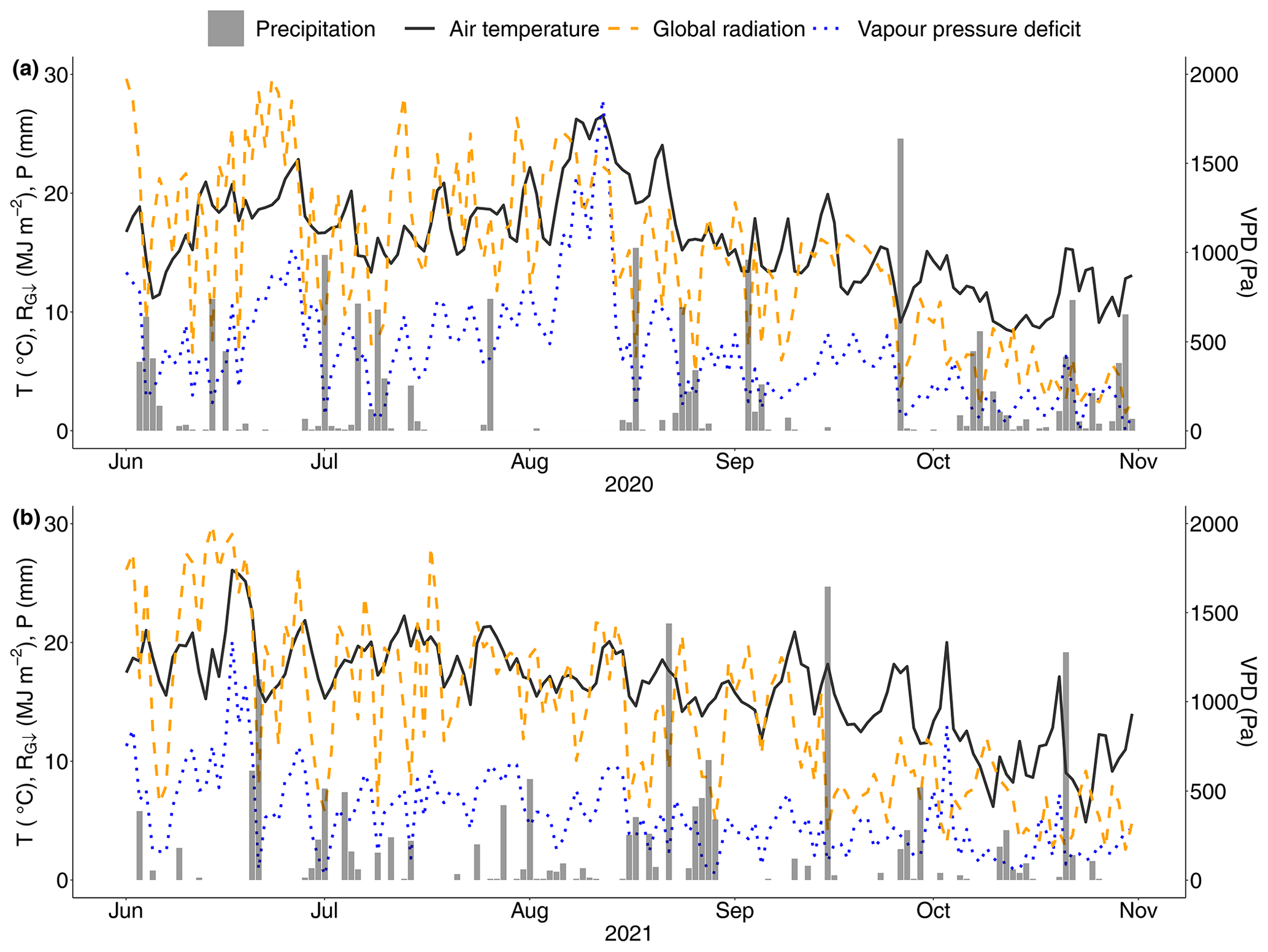
Figure 2 The meteorological conditions during the campaigns in 2020 and 2021. Daily mean values of air temperature, T (°C), and vapour pressure deficit, VPD (Pa), are shown. Additionally, daily sums of precipitation, P (mm), and incoming global radiation, R_G↓ (MJ m⁻²), are shown.

3.2 Lower-cost versus conventional eddy covariance

3.2.1 Diurnal cycle

The diurnal pattern was clearly captured for the CO₂ and LE fluxes by both EC setups and during all campaigns, with CO₂ uptake and water vapour release during the day and CO₂ release and dew fall during the night (Fig. 3). The negative CO₂ fluxes during midday (8–17 h) of the LC-EC were on average 0.56 $\mathrm{\mu }\mathrm{mol}{\mathrm{m}}^{-\mathrm{2}}{\mathrm{s}}^{-\mathrm{1}}$ lower relative to the CON-EC during all campaigns. The positive CO₂ fluxes of the LC-EC were similar to those of the CON-EC in all three campaigns. The mean of the average diurnal CO₂ cycle for both EC setups was positive during both grassland campaigns (1.03 $\mathrm{\mu }\mathrm{mol}{\mathrm{m}}^{-\mathrm{2}}{\mathrm{s}}^{-\mathrm{1}}$ in 2020 and 0.87 $\mathrm{\mu }\mathrm{mol}{\mathrm{m}}^{-\mathrm{2}}{\mathrm{s}}^{-\mathrm{1}}$ in 2021) and was negative during the agroforestry campaign (−0.64 $\mathrm{\mu }\mathrm{mol}{\mathrm{m}}^{-\mathrm{2}}{\mathrm{s}}^{-\mathrm{1}}$). The diurnal pattern of the LE flux was very similar for both EC setups during the grassland campaign in 2020; nevertheless during nighttime the EC setups agreed less, and the diurnal cycle was more noisy. For example, the LE flux of the CON-EC at the agroforestry site was on average 18.4 W m⁻² higher compared to the LE flux of the LC-EC during the first 7 h of the day; however this coincides with time periods when a limited amount of data was available. The LE flux at the grassland site in 2021 has a similar diurnal pattern between EC setups; however the magnitudes were different and opposite to the 2020 campaigns, as in 2021 the daytime LE flux of the LC-EC had a higher magnitude compared to the CON-EC.

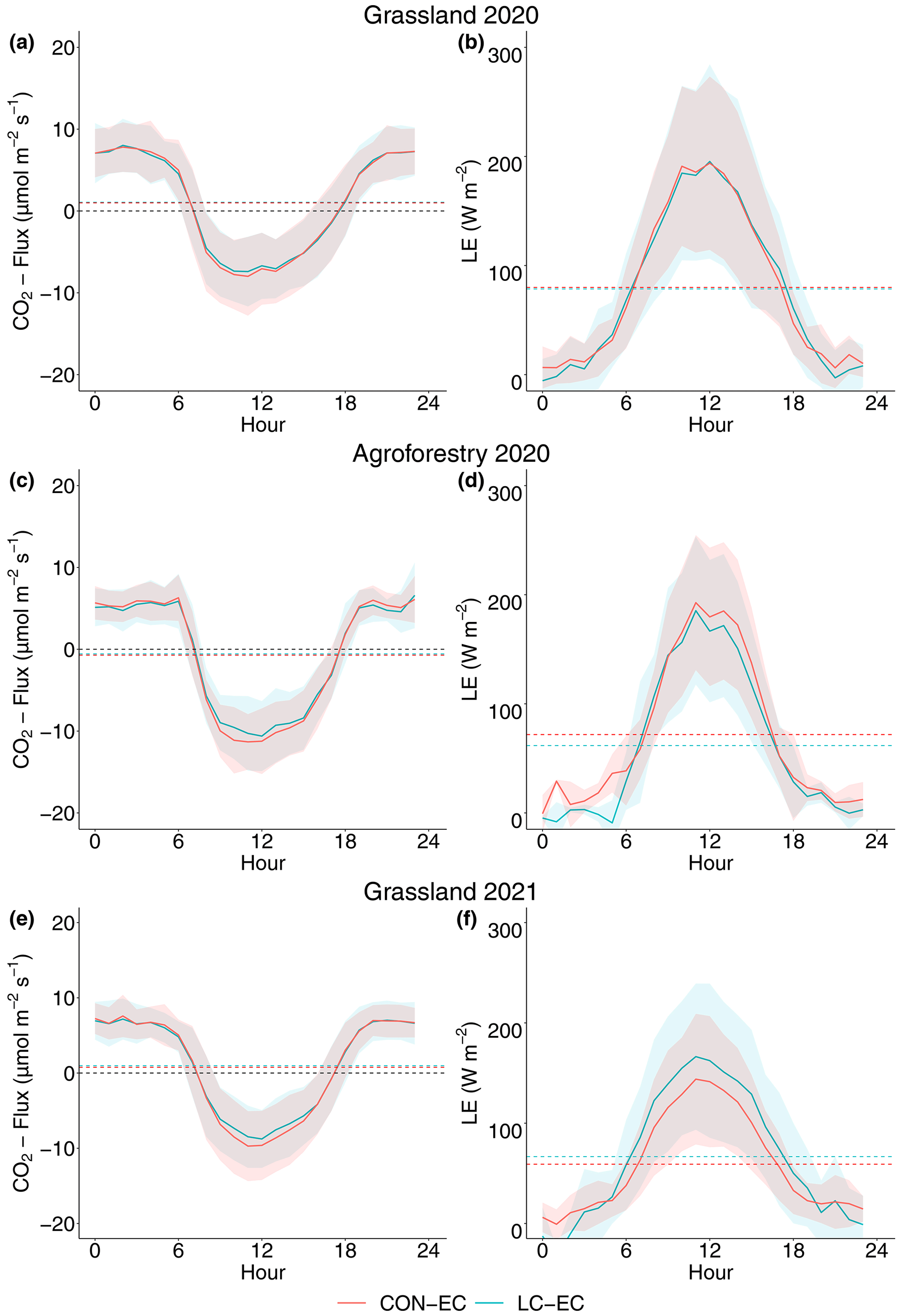
Figure 3 Mean diel cycles of CO₂ and LE fluxes (mean ± standard deviation) based on the entire campaign, measured with the CON-EC (red) and the LC-EC (light blue) setups for the grassland site in 2020 (a, b), the agroforestry site in 2020 (c, d) and the grassland site in 2021 (e, f). The dashed black lines in the figures of the CO₂ flux highlight when the flux is zero and the flux changes sign. A negative flux indicates CO₂ is sequestered, and a positive flux indicates CO₂ is emitted. The dashed red and light blue lines indicate the mean of each diel cycle of the CON-EC and LC-EC, respectively.

The diurnal pattern of the sensible heat flux (H) was also captured and shows very strong agreement between the LC-EC and CON-EC, which share the same ultrasonic anemometer (figure not shown). Nevertheless, the LC-EC has a slightly higher H compared to the CON-EC during midday, reflecting slight differences in the humidity correction for H, and this difference was larger for the grassland sites.

3.2.2 Scatter plots

The CO₂ and LE fluxes of the LC-EC and CON-EC were strongly correlated, with r≥0.95 and r≥0.92 for the CO₂ and LE fluxes, respectively (Table 3). Furthermore, the linear regression results in slopes between 0.93 and 0.96 (R²=0.91–0.95) for the CO₂ fluxes and slopes between 1.01 and 1.23 (R²=0.84–0.91) for the LE fluxes (Fig. 4). The LC-EC CO₂ fluxes were generally lower than the CON-EC CO₂ fluxes, indicated by the slopes from linear regression below 1.0. The agreement for CO₂ fluxes between both EC setups was different for positive and negative fluxes: positive fluxes were overestimated (slope=1.07–1.18), and negative fluxes were underestimated (slope=0.86–0.96) (Table 3). This difference is also confirmed by the non-normally distributed residuals of the linear regressions (p<0.001). The correlation between the LE fluxes of both EC setups was lower compared to the CO₂ fluxes, especially for the grassland sites, which was also visible by the relatively large spread that increases with higher LE fluxes. This increasing spread is also confirmed by the non-normally distributed residuals of the linear regressions (p<0.001). Nevertheless, the slopes for the grassland and agroforestry campaigns in 2020 were good, being 1.01 (R²=0.91) and 1.05 (R²=0.86), respectively. However in 2021, the slope between the LE fluxes at the grassland site was 1.23 (R²=0.84), indicating that the LE flux of the LC-EC setup was 23 % higher compared to the CON-EC setup. The distribution of the positive LE fluxes in 2021 looks very similar to the LE fluxes in 2020; however the magnitude of the LE fluxes does not agree. Furthermore, the negative LE fluxes disagree even more, which indicates differences between EC setups during humid conditions.

Table 3 Additional statistics accompanying the scatter plots from Fig. 4.

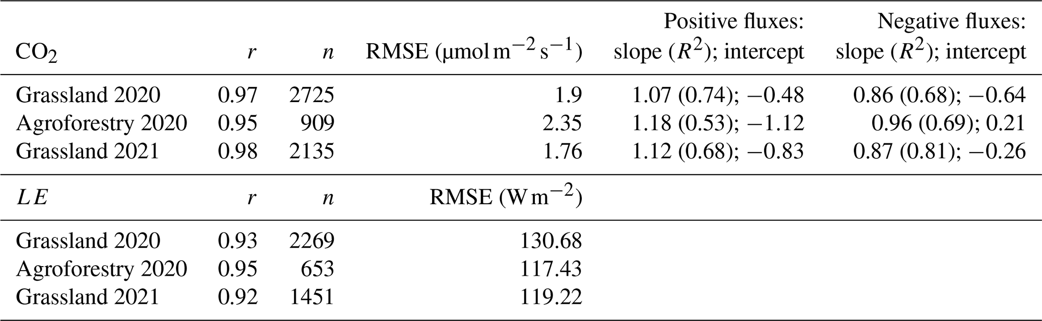
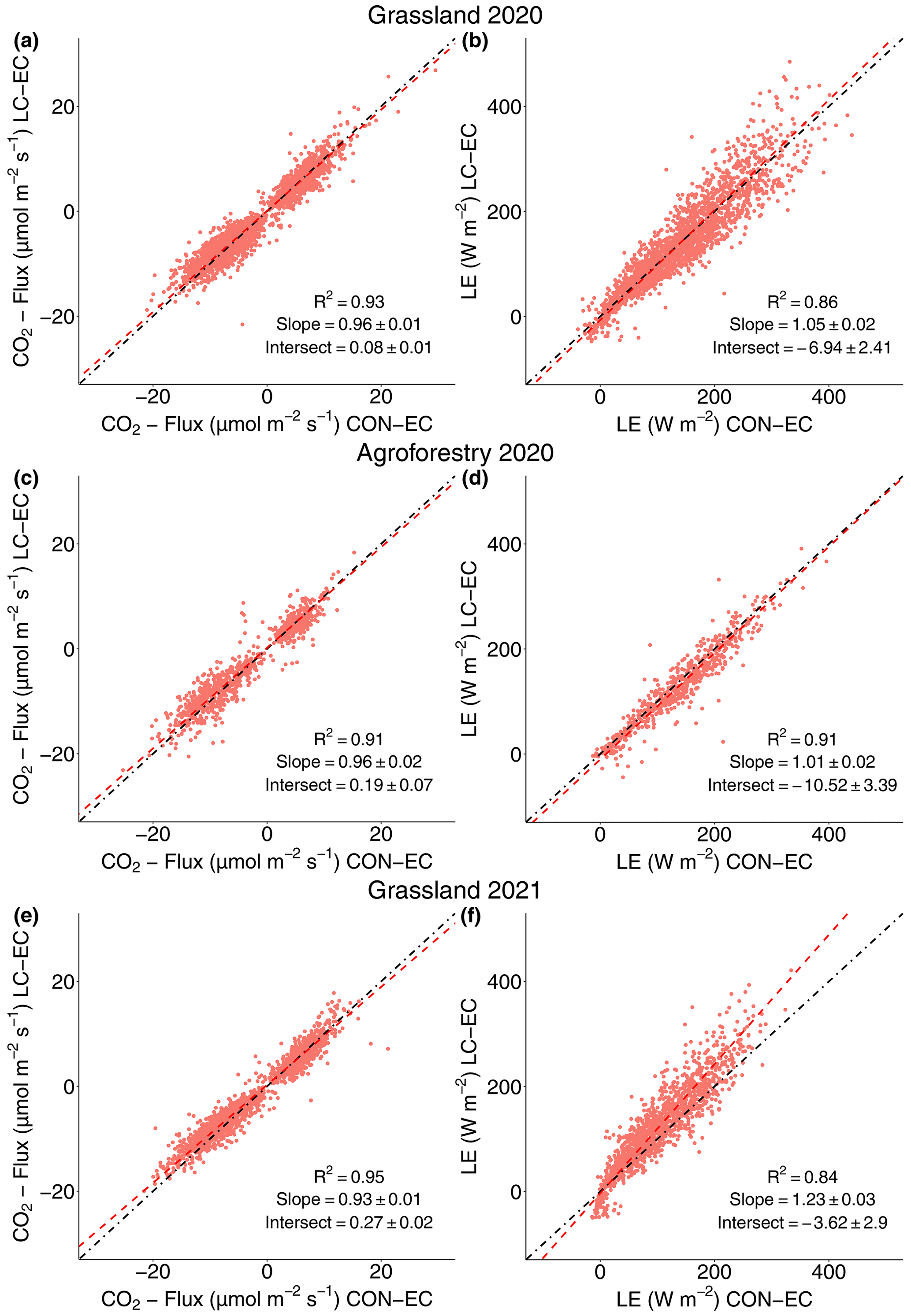
Figure 4 Half-hourly CO₂ and LE fluxes measured with LC-EC versus half-hourly CO₂ and LE fluxes measured with CON-EC for the grassland site in 2020 (a, b), the agroforestry site in 2020 (c, d) and the grassland site in 2021 (e, f). Table 3 includes more statistics accompanying this figure.

The scatter plots of H show a very strong correlation between the LC-EC and EC setups, with r=1.0, which corresponds with the use of the same ultrasonic anemometer (figures not shown). The H fluxes measured with the LC-EC setups were slightly higher compared to the H fluxes measured with the EC setups due to humidity effect corrections, which include measurements of ET, resulting in a slope of 1.03 (R²=1.0) and 1.02 (R²=1.0) for the grassland campaigns in 2020 and 2021, respectively, and a slope of 1.01 (R²=1.0) for the agroforestry campaign.

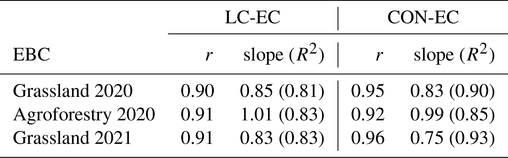
3.2.3 Energy balance closure

The energy balance closure (EBC) at the grassland site in 2020 was similar for both EC setups; however the CON-EC has a higher correlation with the available energy compared to LC-EC (Fig. 5 and Table 4). The agroforestry site in 2020 shows a very high EBC for both EC setups, with a slope of 1.01 and 0.99 for the LC-EC and CON-EC, respectively (Fig. 5 and Table 4). The difference in correlation between the EC setups was smaller at the agroforestry site (Table 4). The EBC at the grassland site in 2021 shows the largest difference between the EC setups (Fig. 5). A slope of 0.83 from the LC-EC was similar compared to 2020. In contrast, the EBC of the CON-EC has a lower slope of 0.75, despite the high correlation (Table 4).

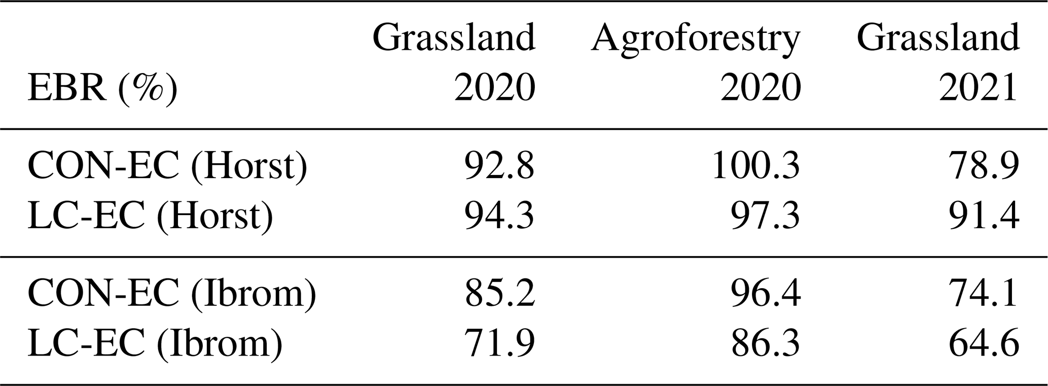
Figure 5 The energy balance closure (EBC) with half-hourly turbulent fluxes (H+LE) measured with the CON-EC (red) and the LC-EC (light blue) setups versus the available energy (R_N−G). The EBC is shown for the grassland site in 2020 (a), the agroforestry site in 2020 (c) and the grassland site in 2021 (e). The cumulative energy balance ratio (EBR) shows the cumulative sum of the half-hourly turbulent fluxes measured with the CON-EC (red) and LC-EC (light blue) setups and the cumulative sum of the available energy (black). The cumulative EBR is shown for the grassland site in 2020 (b), the agroforestry site in 2020 (d) and the grassland site in 2021 (f).

Table 4 Energy balance closure (EBC) for both EC setups and for all three campaigns.

The cumulative energy balance ratio (EBR) at the grassland site in 2020 was similar for both EC setups (Fig. 5 and Table 5). The agroforestry site in 2020 shows a similar and very high EBR closure ratio for both EC setups (Fig. 5 and Table 5). The EBR also shows the largest difference between the EC setups at the grassland site in 2021 (Fig. 5). An EBR closure ratio of 91.4 % from the LC-EC was similar compared to 2020. In contrast, an EBR closure ratio of 78.9 % from the CON-EC was different compared to 2020 (Table 5).

Table 5 Energy balance ratios (EBRs) of the three measurement campaigns and for two different spectral correction methods of Horst (1997) and Ibrom et al. (2007).

3.2.4 Spectral analysis

In general, the spectra of the LC-EC show a stronger decay in energy content compared to the spectra of the CON-EC in the higher-frequency range (i.e. inertial subrange), which was a consequence of the slower sensor response time of the LC-EC sensors (Fig. 6). Furthermore, for both EC setups the H₂O spectra always show more attenuation compared to the CO₂ spectra, and the loss increased during higher-RH conditions, as visualized for RH classes of 50 % and 80 % (Fig. 6b, d and e). However, the H₂O spectra of the heated LC-EC were less affected by the RH conditions compared to the non-heated CON-EC, and the taller AF tower seems less affected by the RH conditions compared to the short grassland towers as well.

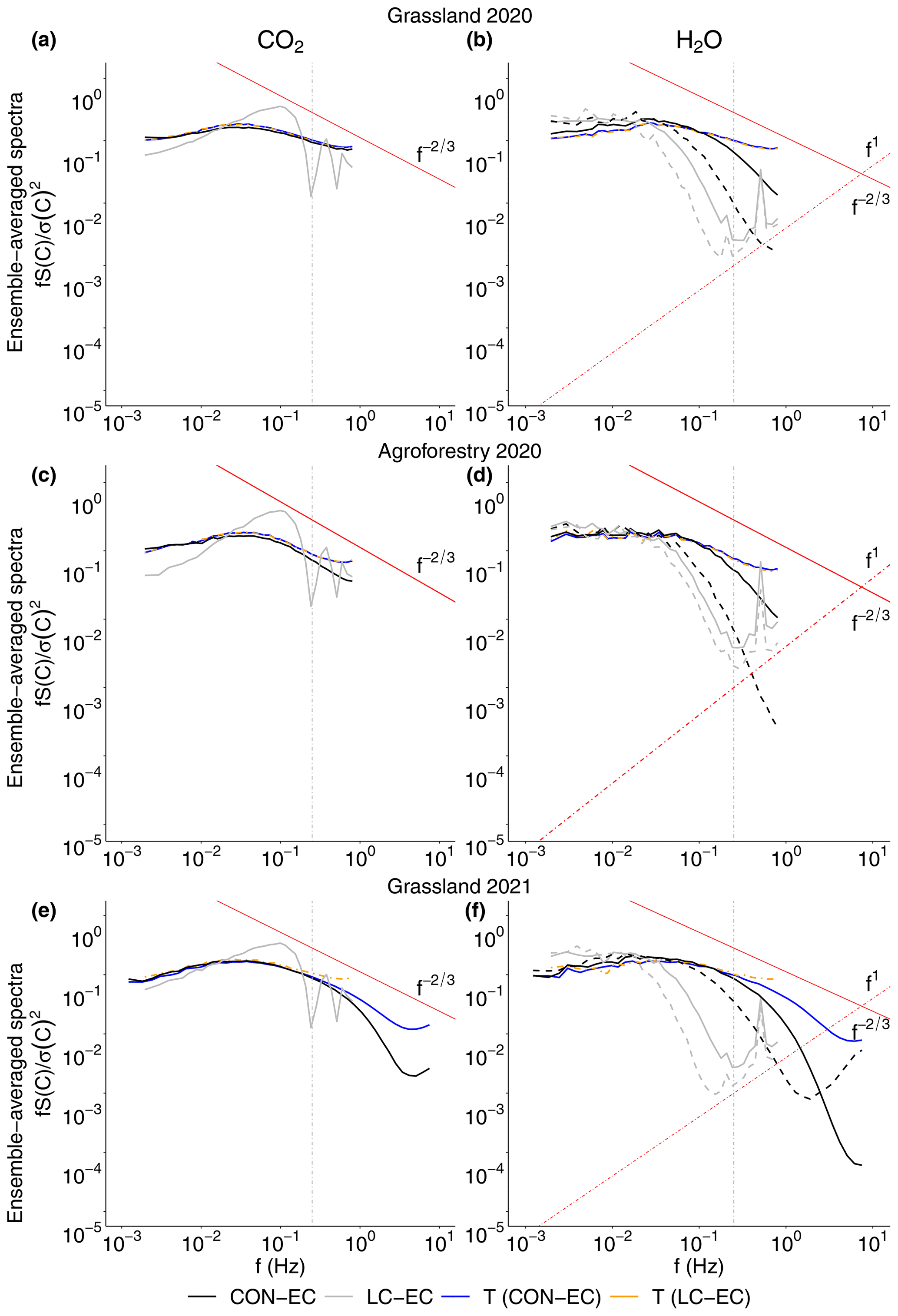
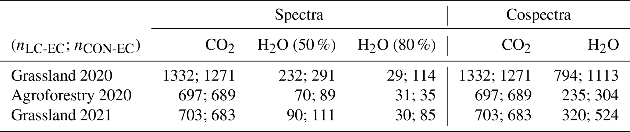
Figure 6 Ensemble-averaged normalized CO₂ (a, c, e), H₂O (b, d, f) and T spectra versus the natural frequency (f). The CO₂ and H₂O spectra of the LC-EC setup (grey) and the CON-EC setup (black) are shown, and the T spectra of the LC-EC setup (dash-dotted orange) and the CON-EC setup (blue) are also shown. The H₂O spectra are shown for relative humidity bins of 45 %–55 % (solid lines) and 75 %–85 % (dashed lines). The spectra for the grassland site in 2020, agroforestry site in 2020 and grassland site in 2021 are shown in panels (a) and (b), (c) and (d), and (e) and (f), respectively. The dash-dotted grey lines at 0.25 Hz are to visualize the fitting range for the high-frequency correction of the LC-EC. The solid red lines with a $-\mathrm{2}/\mathrm{3}$ slope indicate the theoretical decay of the spectra in the inertial subrange, and the dash-dotted red lines with a +1 slope indicate the slope for random white noise. The number of spectra used for the ensemble averages is specified in Table 6.

All the spectra of the CON-EC show the effect of aliasing of the high-frequency signal, clearly visible at the frequencies just under the Nyquist frequency of 1 Hz (2020) and 10 Hz (2021), where the energy content of the power spectra increases in energy due to the folding of the unresolved signal of frequencies higher than the Nyquist frequency of the CON-EC (Stull, 1988; Massman, 2000). At the same time the effect of (random white) noise seems to be apparent in the CO₂ and H₂O spectra as well, expressed by the spectral energy increasing all the way up to a slope of +1. The effect of noise was increasingly present at the H₂O spectra during higher-RH conditions. The LC-EC shows a similar effect of aliasing for the T spectra at frequencies just below 1 Hz, the Nyquist frequency of the LC-EC.

The CO₂ and H₂O spectra of the LC-EC were affected by oversampling, which is visible by the harmonic oscillations in the higher frequencies (Eugster and Plüss, 2010). The oversampling is a consequence of the frequency response time of the CO₂ and H₂O sensors, which is lower than the 2 Hz measurement rate. Based on the frequency response times found by Hill et al. (2017), the oversampling rate can be approximated for the CO₂ and H₂O sensors as follows: $\mathrm{2}/\mathrm{0.74}=\mathrm{2.7}$ and $\mathrm{2}/\mathrm{0.25}=\mathrm{8}$, respectively. The oscillations were clearly visible in both spectra; however the shape of the spectra and oscillations looks different. The CO₂ spectra of the LC-EC show just a harmonic oscillation, and additionally there is an increased spectral energy at lower frequencies due to aliasing. Different from the CO₂ spectra, the H₂O spectra of the LC-EC were affected by random white noise, which results in a loss of sensor signal, visualized by the slope of +1 (Fig. 6). As there is no signal distinguishable from the high amount of noise, there is no unresolved signal to fold back, hence the seemingly unaffected shape of the spectra left of the H₂O sensor's Nyquist frequency. The lack of signal also leads to peaks in the H₂O spectra instead of harmonic oscillations as seen in the CO₂ spectra (Eugster and Plüss, 2010).

The cospectra of the LC-EC also show a stronger decay compared to the spectra of the CON-EC in the higher-frequency range, again a consequence of the slower sensor response time of the LC-EC sensors (Fig. 7). Furthermore, the $\text{Co}\left({\text{wC}}_{{\mathrm{H}}_{\mathrm{2}}\mathrm{O}}\right)$ cospectra for both EC setups show more decay compared to the $\text{Co}\left({\text{wC}}_{{\mathrm{CO}}_{\mathrm{2}}}\right)$ cospectra. The LC-EC $\text{Co}\left({\text{wC}}_{{\mathrm{CO}}_{\mathrm{2}}}\right)$ and $\text{Co}\left({\text{wC}}_{{\mathrm{H}}_{\mathrm{2}}\mathrm{O}}\right)$ cospectra have a higher spectral energy in the lower frequencies compared to the CON-EC due to aliasing of higher frequencies. Moreover, the LC-EC $\text{Co}\left({\text{wC}}_{{\mathrm{CO}}_{\mathrm{2}}}\right)$ and $\text{Co}\left({\text{wC}}_{{\mathrm{H}}_{\mathrm{2}}\mathrm{O}}\right)$ cospectra were quite similar for each setup. Due to the higher measurement height of the AF tower, the cospectra are less attenuated in the high-frequency range, whereas the cospectra from the grassland tower in 2021 show the highest attenuation in the high-frequency range.

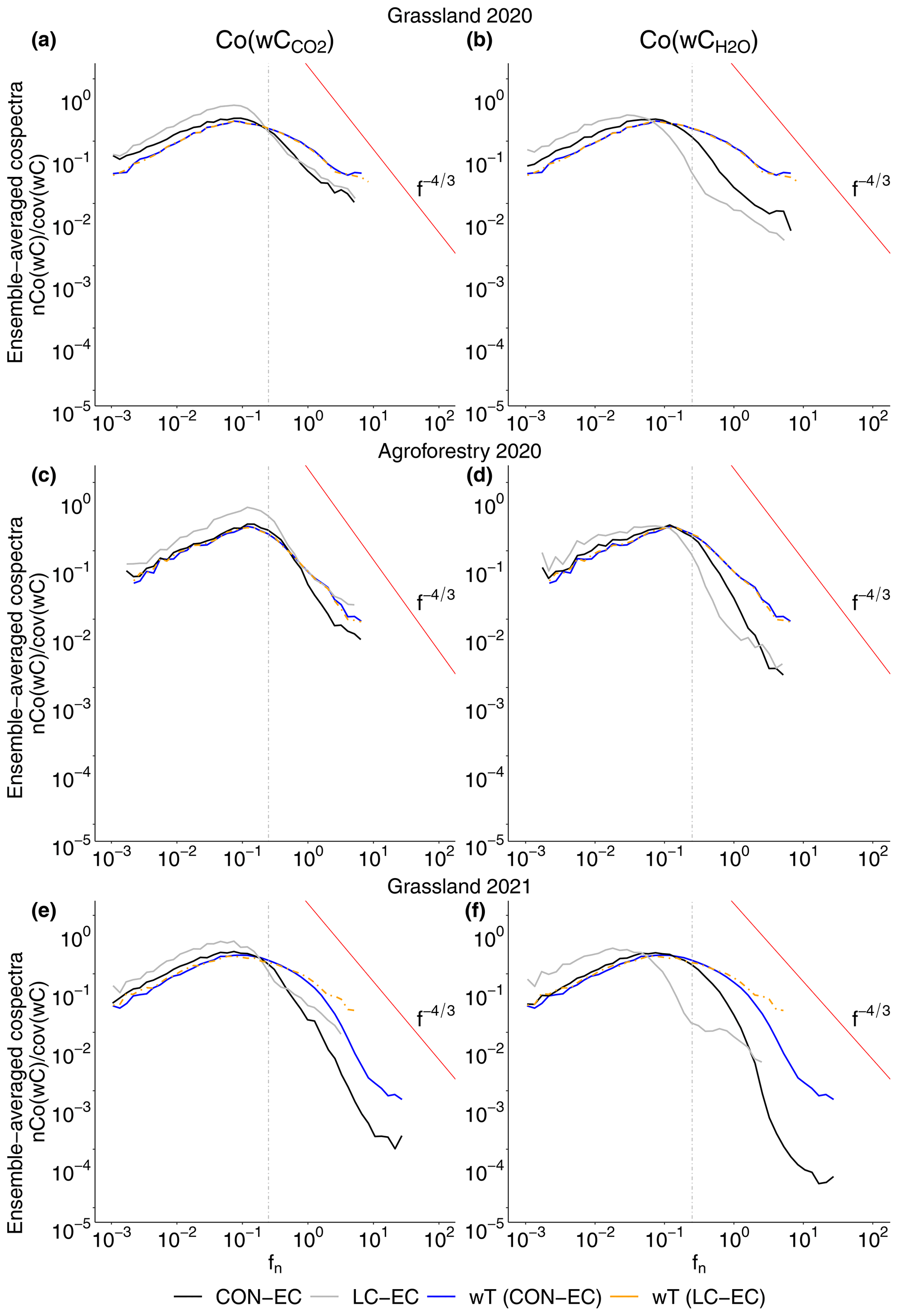
Figure 7 Ensemble-averaged normalized $\text{Co}\left({\text{wC}}_{{\mathrm{CO}}_{\mathrm{2}}}\right)$ (a, c, e), $\text{Co}\left({\text{wC}}_{{\mathrm{H}}_{\mathrm{2}}\mathrm{O}}\right)$ (b, d, f) and Co(wT) cospectra versus the normalized frequency (f_n) for unstable conditions. The $\text{Co}\left({\text{wC}}_{{\mathrm{CO}}_{\mathrm{2}}}\right)$ and $\text{Co}\left({\text{wC}}_{{\mathrm{H}}_{\mathrm{2}}\mathrm{O}}\right)$ cospectra of the LC-EC setup (grey) and the CON-EC setup (black) are shown, and the Co(wT) cospectra of the LC-EC setup (dash-dotted orange) and the CON-EC setup (blue) are also shown. The cospectra for the grassland site in 2020, agroforestry site in 2020 and grassland site in 2021 are shown in panels (a) and (b), (c) and (d), and (e) and (f), respectively. The dash-dotted grey lines at 0.25 Hz are to visualize the fitting range for the high-frequency correction of the LC-EC. The solid red lines with a $-\mathrm{4}/\mathrm{3}$ slope indicate the theoretical decay of the cospectra in the inertial subrange. The number of cospectra used for the ensemble averages is specified in Table 6.

All the cospectra of both EC setups show an increase in spectral energy at the higher end of the frequencies, which seems to be a consequence of the noise sources described in the spectra, namely random white noise, aliasing and oversampling. However, clearly some cospectra were affected earlier by the noise than others, and the harmonic oscillations of the spectra were not visible in the cospectra. The $\text{Co}\left({\text{w C}}_{{\mathrm{CO}}_{\mathrm{2}}}\right)$ and $\text{Co}\left({\text{wC}}_{{\mathrm{H}}_{\mathrm{2}}\mathrm{O}}\right)$ cospectra of the CON-EC in 2021 appear less affected compared to the 2020 cospectra. The Co(wT) cospectra of the LC-EC follow a similar shape compared to the CON-EC Co(wT) cospectra and were the best at the higher AF tower and slightly worse at the grassland towers.

Table 6 Number (n) of CO₂ and H₂O (co)spectra used for the ensemble averages of the LC-EC and CON-EC in Figs. 6 and 7.

3.3 Effect of the spectral correction method on cumulative fluxes

The cumulative CO₂ and ET fluxes show a variety of differences across the spectral correction methods of Horst (1997) and Ibrom et al. (2007), which can be summarized by three observations from Fig. 8:

1. The difference between the spectral correction methods for the cumulative CO₂ fluxes varied between 0.02 %–12.5 %, which was lower compared to the differences between the cumulative ET fluxes, which varied between 5.69 %–38.8 % (Table 7).

2. The differences between the spectral correction methods at the agroforestry site were 0.02 %–0.15 % and 5.69 %–16.4 % for the cumulative CO₂ and ET fluxes, respectively (Table 7). These differences were lower compared to the differences between the spectral correction methods at the grassland sites, which were 0.29 %–12.5 % and 8.43 %–38.8 % for the cumulative CO₂ and ET fluxes, respectively (Table 7).

3. The differences between the spectral correction methods for the cumulative CO₂ and ET fluxes from the CON-EC setups varied between 0.02 %–11.36 %, which was lower compared to the 0.15 %–38.8 % difference between the cumulative CO₂ and ET fluxes from the LC-EC setups (Table 7).

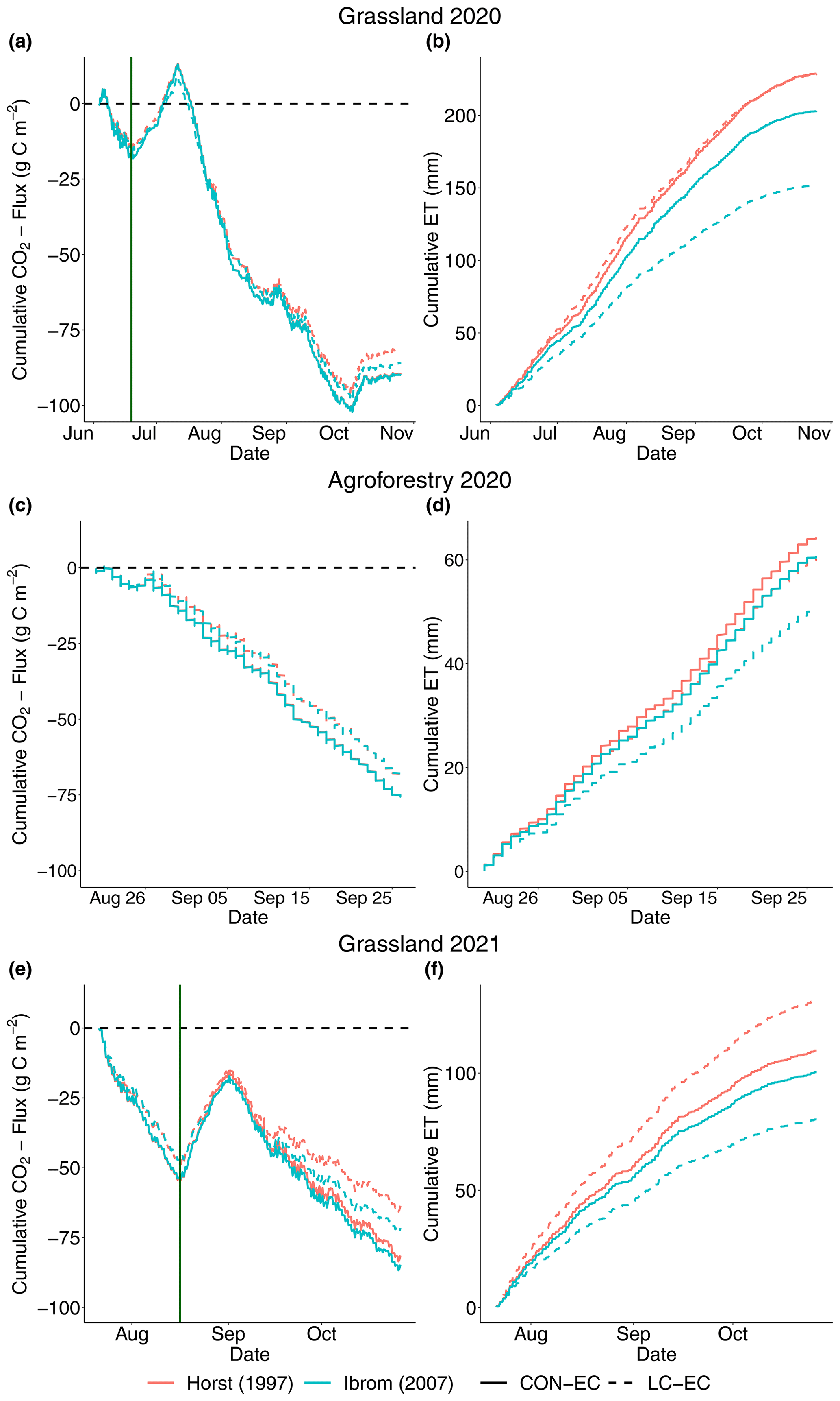
Figure 8 Non-gap-filled cumulative CO₂ (a, c, e) and ET (b, d, f) fluxes of the three measurement campaigns and for two different spectral correction methods of Horst (1997) and Ibrom et al. (2007). The grassland site in 2020 is shown in (a) and (b), the agroforestry site in 2020 is shown in (c) and (d), and the grassland site in 2021 is shown in (e) and (f). The red lines are cumulative fluxes processed with the Horst method, and the light blue lines are cumulative fluxes processed with the Ibrom method. The solid lines are the CON-EC fluxes, and the dashed lines are the LC-EC fluxes. The vertical solid green lines in (a) and (e) indicate when the grassland was mowed. The horizontal dashed black lines in (a), (c) and (e) indicate the transition of the ecosystem being either a CO₂ source (+) or sink (−).

The spectral correction factors (SCFs) of each setup show that these three observations correlate with the magnitude of the SCF (Fig. 9). The higher the SCF, the higher the relative difference between the spectral correction methods. Furthermore, the SCF was always higher for the Horst method compared to the Ibrom method (Fig. 9). Accordingly, the Horst method leads to a higher closure of the energy balance compared to the Ibrom method (78.9 %–100.3 % versus 64.6 %–96.4 %, respectively) (Table 5).

Figure 9 Boxplots of the CO₂ (a, c, e) and H₂O (b, d, f) spectral correction factors (SCFs) of the three measurement campaigns and for two different spectral correction methods of Horst (1997) and Ibrom et al. (2007). The grassland site in 2020 is shown in (a) and (b), the agroforestry site in 2020 is shown in (c) and (d), and the grassland site in 2021 is shown in (e) and (f). The red boxes are the SCFs of the Horst method, and the light blue boxes are the SCFs of the Ibrom method and are shown for both EC setups separately. For the boxplots only the SCFs of the quality-controlled data are used. The number of measurements (n) used for the four boxplots is shown in the upper-left corners, and the value above each boxplot indicates the mean SCF.

The ET flux of the grassland campaign in 2021 was different compared to the 2020 campaigns for two reasons (Fig. 8f). (i) The difference between the spectral correction methods for the LC-EC setup was 5.3 % higher in 2021 compared to the same grassland in 2020 (Table 7). (ii) In contrast, the difference between the spectral correction methods for the CON-EC was 1.42 % lower, and the H₂O SCFs in 2021 were lower and show less spread compared to both campaigns in 2020 (Fig. 9). As a consequence of the lower SCFs, the energy balance ratio with the CON-EC at the grassland in 2021 was only 74.1 %–78.9 % compared to 85.2 %–92.8 % in 2020 (Table 5). Finally, the CO₂ flux of the CON-EC in 2021 looks reasonable and has a higher SCF compared to 2020.

3.4 Ecological application

3.4.1 Cumulative fluxes

Both EC setups capture the temporal variability of CO₂ fluxes, such as diel patterns (Fig. 3) and mowing events, e.g. on 19 June 2020 and 16 August 2021, well (Fig. 8). Both EC setups also capture the temporal variability of ET, showing that ET decreases towards the end of the growing season.

Even though the non-gap-filled cumulative fluxes of the LC-EC and EC agree quite well (Fig. 8), the magnitudes of the cumulative fluxes show a difference between EC setups, varying between 0.23 %–28.0 % for the Horst method (Table 7), which was an aggregation of structural offsets between the CO₂ and ET fluxes measured by the LC-EC and CON-EC during parts of the day (Fig. 3). For the ET measurements the difference between the EC setups was on average 18.6 % higher with the Ibrom method than with the Horst method (Table 7). In contrast, for the CO₂ fluxes the difference between the EC setups was equal or higher with the Horst method than with the Ibrom method.

Table 7 The relative differences in the non-gap-filled cumulative CO₂ and ET fluxes between the LC-EC and CON-EC setups and between the Horst (1997) and Ibrom et al. (2007) spectral correction methods. The relative differences were calculated based on the final value of the cumulative sums of CO₂ and ET or each EC setup and spectral correction method.

3.4.2 Agroforestry versus grassland

In 2020 the grassland and agroforestry sites were measured simultaneously for about 1 month, and in Fig. 10 the gap-filled cumulative CO₂ and ET fluxes for this period are compared. During this month, the agroforestry site was a carbon sink of −67.9 g C m⁻², and the grassland site was a carbon source of 37.7 g C m⁻², based on the average cumulative CO₂ sequestration of both EC setups (p<0.001 for LC-EC and CON-EC). The CO₂ flux difference between the EC setups was smaller than the ecosystem difference, being 19.6 and 8.1 g C m⁻² for the grassland and agroforestry sites, respectively. Similarly, the average gap-filling uncertainty for both EC setups was also smaller than the ecosystem difference, being 3.2 and 3.6 g C m⁻² for the grassland and agroforestry sites, respectively. The cumulative ET of both EC setups shows a less clear message – the ET was higher for both EC setups at the grassland site than at the agroforestry site; however the CON-EC was 14.4 mm higher (p<0.001) and the LC-EC was 3.1 mm higher (p>0.05). The average gap-filling uncertainty for both EC setups was 1.5 and 1.4 mm for the grassland and agroforestry sites, respectively. Furthermore, for the CO₂ and ET fluxes the difference between the LC-EC and CON-EC was larger at the grassland site (p<0.001 for CO₂ and ET). The difference in cumulative sums between the agroforestry and grassland site was smaller with the LC-EC setup (p<0.001 for CO₂ and ET).

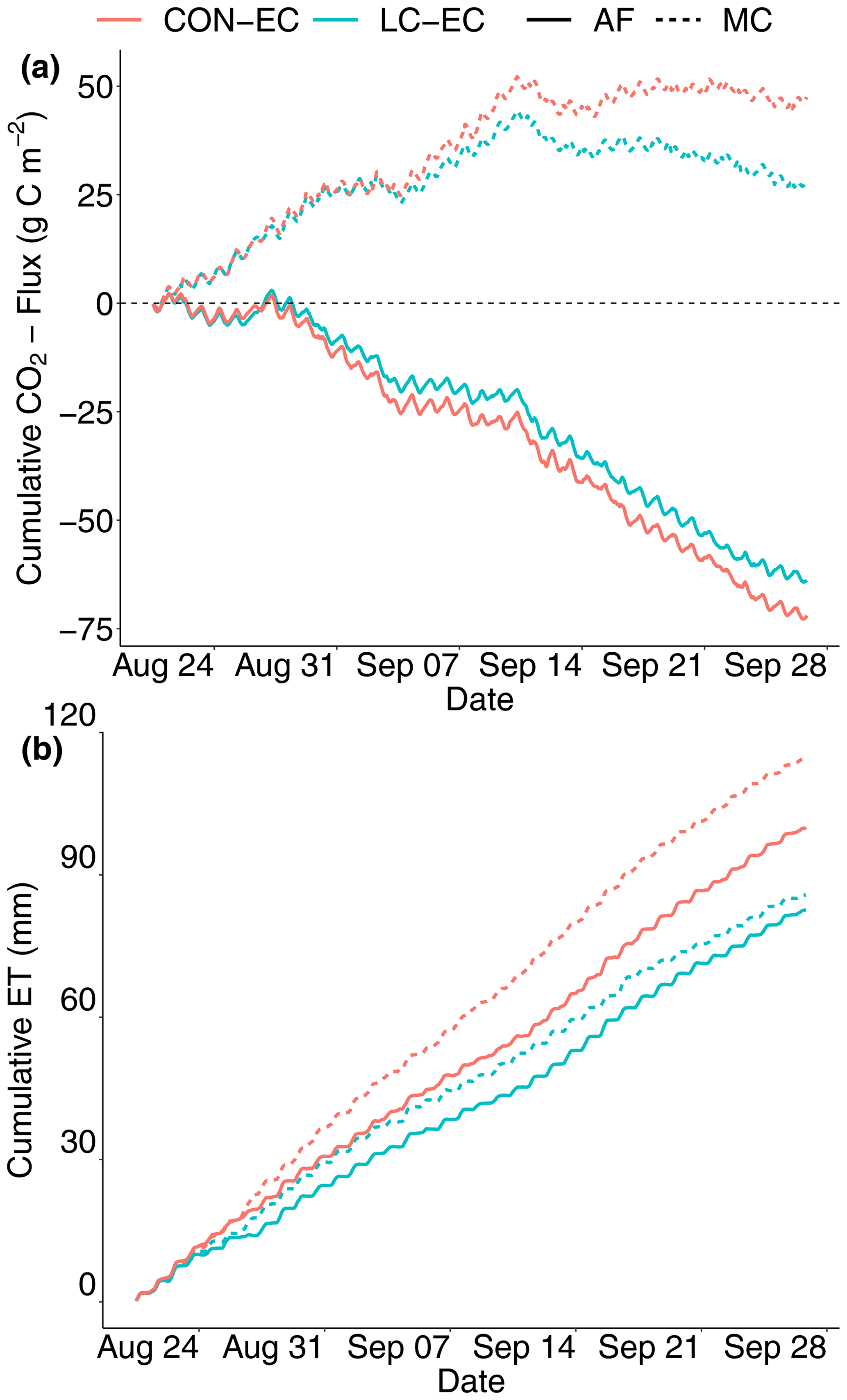
Figure 10 Gap-filled cumulative CO₂ (a) and evapotranspiration (ET) (b) fluxes of the agroforestry (AF) and grassland sites during the period when they were measured simultaneously in 2020. The red lines are the CON-EC fluxes, and the light blue lines are the LC-EC fluxes. The dashed lines are the grassland site, and the solid lines are the agroforestry site. The horizontal dashed black line in (a) indicates the transition of the ecosystem being either a CO₂ source (+) or sink (−).

4 Discussion

4.1 Technical characterization

The current study showed that the LC-EC was able to capture the diel pattern and ecosystem response of the CO₂ and LE fluxes observed at the grassland and agroforestry grassland sites by the CON-EC. The stronger attenuation of the LC-EC led to consistently higher spectral corrections for the LC-EC setup compared with CON-EC (Fig. 9). Nevertheless, the LC-EC setup showed a strong correlation with the CON-EC, with r=0.95–0.98 and r=0.92–0.95 for the CO₂ and LE fluxes, respectively (Fig. 4). The LC-EC CO₂ flux was slightly lower compared to CON-EC, indicated by the linear regression slopes of 0.93–0.96 (R²=0.91–0.95). The LC-EC LE fluxes in 2020 were slightly higher compared to CON-EC, indicated by linear regression slopes of 1.01 and 1.05 (R²=0.84–0.91), and had similar diel cycles. The LE fluxes in 2021 did not agree well, and this observation is discussed in more detail in Sect. 4.1.4.

4.1.1 Comparison to other lower-cost eddy covariance studies

To put the results of the current study in perspective, a comparison is made with the few existing recent studies comparing CO₂ and H₂O fluxes of an LC-EC setup and a CON-EC setup.

The study of Hill et al. (2017) compared a predecessor of the current LC-EC setup with an open-path LI-7500 IRGA at a 4.25 m tall tower on a pasture in Dumfries and Galloway, UK. This predecessor had a higher flow rate of approximately 75 L min⁻¹, but despite the different CON-EC IRGA and a higher flow rate, their results agree quite well with the current study. Their CO₂ fluxes had better agreement in magnitude, with a linear regression slope of 1.03 and 0.983 compared to 0.87–0.93; however the coefficient of determination (R²) between their EC setups was lower, with an R² of 0.86 and 0.72 compared to an R² between 0.91 and 0.95. It has to be noted that the amount of QC in their study was minimal, which probably led to lower R² as compared to the extensive QC in the current study. The H₂O fluxes of both studies were quite similar, with a linear regression slope of 1.06 (R²=0.89) compared to 1.02 (R²=0.9) and 1.03 (R²=0.85). Even with the turbulent conditions inside the sampling tube and the higher flow rate, the average spectral correction factors (SCFs) of the CO₂ flux of Hill et al. (2017) were higher compared to our study (1.52–1.55 compared to 1.12–1.3). The SCF of the LE flux of Hill et al. (2017) was 2.33, which was lower than the SCF at the grassland towers of 3.37 and 4.18 but higher than the SCF of 1.82 at the agroforestry tower. Furthermore, they noted that the agreement of the LC-EC CO₂ flux with the LI-7500 got worse with lower-magnitude CO₂ fluxes, which was probably a consequence of a lower signal-to-noise ratio.

The study of Cunliffe et al. (2022) used the exact same LC-EC enclosure as the current study, at a 6.0 m tall tower in the northern Chihuahuan Desert, USA. The fluxes were compared with a LI-7500; however the measurements do not take place at one and the same tower but at four nearby towers. Furthermore, the fluxes were affected by a low signal-to-noise ratio due to the low magnitude of fluxes in a dry desert ecosystem. For fluxes at a daily timescale, their LC-EC LE fluxes showed a worse performance compared to CON-EC, with the LC-EC LE fluxes being approximately 6 %–22 % lower compared to the LC-EC LE fluxes that were 2 %–3 % higher for half-hourly fluxes. However, their cumulative ET – including gap filling – looks similar to the ET measurements at the agroforestry tower of the current study. The CO₂ flux of Cunliffe et al. (2022) was severely affected by the low magnitude of CO₂ fluxes, which led to a low correlation between the LC-EC and CON-EC setups, and LC-EC CO₂ fluxes being lower with a slope of approximately 0.48 for fluxes at a daily timescale compared to a slope of 0.87–0.93 for half-hourly fluxes. The clearly noisy CO₂ fluxes of Cunliffe et al. (2022) also result in a high uncertainty in the cumulative CO₂ fluxes.

The parallel study of Callejas-Rodelas et al. (2024) used the same LC-EC enclosure as the current study, at a 3.5 m tall tower on a crop field in Wendhausen, Germany. The fluxes of the three LC-EC setups at one single tower were also compared with a LI-7200; however the flux calculations were performed using EddyUH software (Mammarella et al., 2016), and the high-frequency corrections were applied following the method from Mammarella et al. (2009). Their non-gap-filled CO₂ fluxes across the LC-EC setups had better agreement in magnitude with linear regression slopes between 0.95–1.05 compared to 0.93–0.96 but a similar high R² between the EC setups of 0.88–0.92 compared to 0.91–0.95. Their non-gap-filled H₂O fluxes across the LC-EC setups performed worse, with lower slopes between 0.88–0.99 compared to 1.01–1.05 but similar R² of 0.85 compared to 0.86–0.91 (LC-EC setup with issues excepted). As a consequence of the lower LE fluxes for both the LC-EC and the CON-EC in their study, the energy balance closure was worse compared to the current study (66 %–74 % compared to 83 %–85 %). Moreover, the LI-7200 from Callejas-Rodelas et al. (2024) potentially also underestimates the LE flux, as in the current study, indicated by the low EBC and the large difference in ET compared to agroforestry (Sect. 4.1.4).

For an even wider perspective, the study of Polonik et al. (2019) is useful, comparing CO₂ and H₂O fluxes of five types of conventional IRGAs and three types of ultrasonic anemometers on a 4 m tall tower at the edge of an alfalfa field in Davis, California. Even though these were all conventional, high-cost EC setups, the spread of the linear regression slope between EC setups varied between 0.92 and 1.08 for CO₂ fluxes and 0.74 and 1.36 for H₂O fluxes, depending on the spectral correction method. Hence, all the linear regression slopes of the CO₂ and H₂O fluxes of the current study fit within this range, even though the tower of the current study was 1 m lower. Finally, in the current study we compared the LC-EC with a LI-7200; however the study of Polonik et al. (2019) highlights that there is no absolute truth, which means care is needed when comparing the performance of EC setups.

4.1.2 Detailed technical characterization

The EBCs of both EC setups during the two grassland campaigns in the current study fit within the observed range of 0.86 ± 0.20 for grasslands of the FLUXNET database (Stoy et al., 2013). Nevertheless, the EBC of the CON-EC in 2021 was lower and agreed better with the EBC of a wetland of 0.76 ± 0.13 (Stoy et al., 2013). The EBC of the agroforestry site was on average 16.3 % higher compared to the grassland sites, which can be explained by the more heterogeneous landscape, which results in increased turbulent conditions and a higher u^* at the agroforestry tower (Franssen et al., 2010; Stoy et al., 2013). Moreover, not measuring the storage components (soil, air and biomass) of the energy balance at the agroforestry site might give a biased image of the EBC, as the tree strips could potentially store energy.

When an EC tower is taller, the high-frequency eddies become less important and the cospectrum peak and the energy-containing eddies shift to lower frequencies, and, oppositely, closer to the ground the higher-frequency eddies are more important (Moncrieff et al., 1997; Reitz et al., 2022). This effect was clearly seen when the high-frequency spectral correction factors of the 10 m tall agroforestry tower were compared to those of the 3 m grassland tower (Fig. 9). In 2020, the CO₂ and H₂O SCFs were on average 7 % and 39 % lower for the LC-EC at the agroforestry site. This effect was larger for the LC-EC than for the CON-EC because at a tall tower it is less problematic that the LC-EC is not able to measure the high-frequency eddies due to a higher occurrence of low-frequency eddies, which seem to better fit the slower response time of the CO₂ and RH sensor (Markwitz and Siebicke, 2019). Furthermore, it is important to note that the high-frequency spectral correction (method) also becomes less important when the tower is taller, as there is less loss which needs to be compensated for (Mauder and Foken, 2006). To summarize, the performance of the LC-EC probably improves with increasing tower height; however this must be possible within the targeted ecosystem, as the footprint size increases with tower height.

One of the differences between the EC setups was the flow rate and the consequent laminar or turbulent flow regime inside the inlet tube. Turbulent flow conditions inside the inlet tubes are generally preferred because the high-frequency attenuation is less compared to laminar flow conditions (Leuning and Moncrieff, 1990; Suyker and Verma, 1993; Moncrieff et al., 1997). Nevertheless, the tube attenuation can be characterized by the Reynolds number, and turbulent flow conditions do not per definition lead to less attenuation compared to laminar flow conditions (Massman, 1991). Furthermore, a higher flow rate requires more power and more cleaning maintenance due to the increase in pollutants inside the tubing and filters (Moncrieff et al., 1997). Also, it needs to be considered that tube attenuation affects the higher frequencies, which are not measured by the LC-EC setup anyway, due to the slow response of the CO₂ and H₂O sensors. Therefore, higher turbulent flow rates might not reduce the attenuation of the LC-EC that much compared to CON-EC setups, as observed when the SCFs of the current study were compared with the SCFs of Hill et al. (2017). Moreover, it was noteworthy that the agroforestry site, with a 9 m long tube, has a lower attenuation than the grassland site, with a 2 m long tube, which shows that other design aspects, such as height, might be more important for the LC-EC setup (Leuning and Moncrieff, 1990). In general, a shorter tube length would likely reduce the flux attenuation and the time lag, something which can be considered in future designs of the LC-EC setup (Leuning and Moncrieff, 1990).

Finally, two considerations for future LC-EC studies are as follows: (i) an LC-EC design with shorter inlet tubes would probably reduce attenuation. Additionally, the study by Callejas-Rodelas et al. (2024) suggests heating these shorter inlet tubes, in addition to heating the enclosure, to prevent condensation and potential erroneous data. (ii) In the current study only the highest-quality data (Flag 0) were used, which for both EC setups led to discarding 51 %–77 % of the data, which is not uncommon, especially at nighttime (Papale et al., 2006; Mauder et al., 2013). Nevertheless, for future long-term ecosystem flux analysis this would lead to large gaps, and therefore using high- and moderate-quality data (Flags 0 and 1) is recommended. This would increase the noise of the fluxes; however the study by Callejas-Rodelas et al. (2024) shows that the correlation between the LC-EC and CON-EC was still good with such quality control, and instead 29 %–38 % of the data were discarded.

4.1.3 Spectral characterization

The spectra and cospectra are described in detail in Sect. 3.2.4; however the distortions due to noise, aliasing and oversampling are discussed more elaborately in this section.

The random white noise and aliasing effects were visible in all spectra and cospectra; however these do not affect the flux calculations. The random white noise is not correlated with the vertical wind speed and therefore makes no systematic contribution to the fluxes (Rummel et al., 2002). Aliasing is the folding of an unresolved signal above the Nyquist frequency into frequencies below the Nyquist frequency, which distorts the shape of the (co)spectra, but this does not influence the total flux calculations (Stull, 1988; Massman, 2000). Aliasing can occur because the Nyquist frequency is lower than the sensor response time (Stull, 1988), but aliasing in the low-frequency range is also possible when the sensor incorrectly represents the energy of the higher frequencies (Markwitz and Siebicke, 2019). The aliasing of the cospectra in the lower-frequency range and an increase in spectral energy in the high-frequency range were also observed by the LC-EC setup of Markwitz and Siebicke (2019).

The effect of oversampling was clearly visible in the LC-EC CO₂ and H₂O spectra. The LC-EC CO₂ spectra were affected by a combination of oversampling and aliasing, something which is observed by Eugster and Plüss (2010) for high oversampling rates. The strong oscillations are not uncommon; however the location of the aliasing was different than that of the standard aliasing just below the sampling Nyquist frequency, being either 1 Hz or 10 Hz, as described before. Based on the peaks of the oscillations it was possible to determine the sensor Nyquist frequency and the response time of the CO₂ sensor, as described by Eq. (1) in Sect. 4.3 of Eugster and Plüss (2010). The first peak of the oscillations was at ∼0.37 Hz, which can be converted into a sensor Nyquist frequency of ∼0.123 Hz and a sensor response time of ∼0.25 Hz. A 4 s sensor response time fits the length of the complete measurement sequence of the GMP343 CO₂ sensor, which is 4 s (Hill et al., 2017). Nevertheless, a single measurement of the GMP343 within the complete sequence lasts 1.36 s, and this was found to be the optimal time response for the frequency corrections by Hill et al. (2017) and Callejas-Rodelas et al. (2024). The LC-EC H₂O spectra were affected by a combination of oversampling and the absence of signal in the frequencies higher than ∼0.25 Hz. The absence of signal leads to the observed peak at ∼0.5 Hz in the spectra instead of oscillations (Eugster and Plüss, 2010). Furthermore, the H₂O spectra confirm the observed sensor response time of 0.25 Hz by Hill et al. (2017), as beyond this frequency no signal is distinguishable from noise.

4.1.4 Underestimation of the latent heat flux in 2021

The general characterizations of the LC-EC and CON-EC fluxes are discussed in the previous section; however the H₂O flux of the CON-EC in 2021 is discussed in more depth since agreement between the LC-EC and CON-EC was poor.

First, it was not expected that the SCF for the LE flux from the CON-EC setup would be lower in 2021 compared to 2020, as Fratini et al. (2012) predict that a higher RH and wind speed would lead to a higher SCF for the LE flux, something which was not observed in the current study for either spectral correction method (Fig. 9). On the other hand, Barr et al. (1994) and Brotzge and Crawford (2003) measured and De Roo et al. (2018) modelled the decrease in EBC when the Bowen ratio decreased. The Bowen ratio decreases when the $\frac{{\text{ET}}_{\text{actual}}}{{\text{ET}}_{\text{potential}}}$ ratio increases (Eltahir, 1998). As 2021 was wetter and colder compared to 2020, the actual ET was closer to the potential ET, and therefore the Bowen ratio was lower in 2021, which could explain why the LI-7200 performed worse in 2021. Additionally, Stoy et al. (2013) report that wetlands, with likely more humid conditions and a lower Bowen ratio compared to less wet environments, on average have a lower EBC compared to normal grasslands. Recently, the study of Zhang et al. (2023) also showed the consistent underestimation of LE fluxes in the high-quality FLUXNET2015 data set, especially for closed- and enclosed-path sensors during high-RH conditions above 70 %. In the current study, 51 % of the quality-controlled LE data in 2021 had an RH inside the IRGA above 70 % compared to 31 % in 2020, confirming that the data in 2021 were more likely affected by similar issues.

More specific to the LI-7200, the study of Metzger et al. (2016) suggests heating the inlet to prevent having RH levels inside the IRGA above 60 %, which is considered problematic. In the current study, 77 % and 54 % of the quality-controlled LE measurements in 2021 and 2020 consist of an RH level inside the IRGA higher than 60 %, respectively. In retrospect, heating the LI-7200 could have prevented the issue visible with the LE data in 2021, as the heated LC-EC enclosure also does not show this issue. Nevertheless, this is not a guarantee that issues will not occur, as the study of Perez-Priego et al. (2017) used an insulated and heated inlet but still reported strong underestimations of up to 35 % of the LE flux using a LI-7200. These large errors occurred especially during humid and high-RH conditions in the growing season, and the underestimation was much larger at the shorter tower (1.5 m) compared to the tall tower (15 m) (Perez-Priego et al., 2017).

It is not possible to identify a clear cause of the LE underestimations in 2021 and why these did not occur in 2020. It is clear that the difference in LE and EBC between the CON-EC and LC-EC increases with higher RH in 2021 (data not shown), which confirms that the effect of water plays an important role in the EBC (Stoy et al., 2013). However, the same effect was not visible in 2020 during high-RH conditions, which suggests that the magnitude of RH is not the only important element. Additionally, the study of Zhang et al. (2023) mentions the importance of spectral correction methods, which take into account the effect of RH, but at the same time also notes that potentially these also do not fully correct for the observed biases. The current study confirms that both the Horst (1997) and the Ibrom et al. (2007) spectral correction methods lead to an underestimation of the LE flux in 2021. This suggests that the issue was independent of the spectral correction method but could for example point at a transfer function that represents the actual attenuation poorly. For example, De Ligne et al. (2010) and Emad (2023) argued that using a first-order linear filter to fit the non-linear behaviour of the H₂O spectral attenuation might not be the most accurate. Nevertheless, the linear infinite impulse response (IIR) fit obtained with EddyPro in 2021 was not perfect but also not very poor or worse than in 2020, which suggests that something other than the spectral correction might play a role in the observed underestimations of the latent heat flux (Fig. A1).

4.2 Effect of the spectral correction method

The results showed that the relative effect of the spectral correction method on the flux magnitude increases with higher spectral correction factors or, in other words, with an increasing loss of high-frequency signal. When the relative importance of the spectral correction method increases, small systematic differences between spectral correction methods are added up, and the difference between spectral methods and the total uncertainty of the flux increases (Mauder and Foken, 2006; Reitz et al., 2022). As the LC-EC per definition has stronger loss of high-frequency signal, applying the right spectral correction method is more important compared to CON-EC. Based on our results, and especially the better energy balance closure and energy balance ratio, the Horst (1997) method was chosen as the preferred spectral correction method in the current study, even though the Ibrom et al. (2007) method was designed for closed-path EC setups. As the LC-EC fluxes still deviated from the CON-EC, it would be interesting to test a wide variety of other spectral correction methods in the future, especially because the system design of the LC-EC is different from that of CON-EC setups, which have been used and thoroughly tested in the past (Polonik et al., 2019; Reitz et al., 2022).

4.3 Ecological application

The LC-EC setup was able to measure the CO₂ and LE fluxes above the grassland and agroforestry grassland, including ecosystem disturbances such as grass mowing. During simultaneous measurements at the agroforestry and grassland sites, there was a significant difference in cumulative carbon uptake over a 1-month period. Despite the short measurement period and the gap-filling uncertainty, it was likely that the agroforestry site sequestered more carbon, as the recent study by Veldkamp et al. (2023), which includes the grassland site of the current study, showed that there was a significant difference in carbon sequestration between agroforestry and monoculture grasslands. Furthermore, trees on agricultural land globally contribute significantly to carbon uptake and storage (Zomer et al., 2016). During the same period there was a partly significant difference in cumulative ET, similar to what was observed by Markwitz et al. (2020) at several agroforestry sites in Germany.

4.4 Costs of and considerations for a lower-cost eddy covariance setup

The application of our LC-EC setup is less standardized compared to the more commonly used LI-7200. Nevertheless, the current study and the parallel study by Callejas-Rodelas et al. (2024) showed that LC-EC setups can be an alternative to CON-EC and provided elaborate examples on how to post-process the LC-EC data for other users. The post-processing of the LC-EC data requires some extra steps, which are easy to implement, and the LC-EC flux calculations take only approximately 10 % of the time compared to the CON-EC flux calculations due to the lower measurement frequency. The main advantage is the approximately 75 % reduction in material costs (Cunliffe et al., 2022), as our LC-EC is approximately EUR 11 000 compared to more than EUR 40 000 for the CON-EC with a LI-7200 (Callejas-Rodelas et al., 2024). Furthermore, the LC-EC setups have a lower power consumption, which makes them suitable for remote locations with only solar power available (Callejas-Rodelas et al., 2024). The LC-EC also requires maintenance and needs to be cleaned regularly; however calibrating the GMP343 with Vaisala software is straightforward, and the HIH-4000 is long lasting without calibration (Callejas-Rodelas et al., 2024). Finally, future LC-EC studies can contribute to further standardization and optimization of the employment and flux processing.

5 Conclusions

The current study showed at an agroforestry and grassland site in a temperate ecosystem that lower-cost eddy covariance (LC-EC) can be a cheaper alternative to the costly conventional EC (CON-EC). There was a strong correlation between the CO₂ and latent heat flux measurements of the closed-path LC-EC and the CON-EC with an enclosed-path LI-7200. The LC-EC CO₂ fluxes were slightly lower in magnitude than those of the CON-EC, and the LE flux was equal for both EC setups in 2020. In 2021, the LE flux of the LC-EC was of a similar quality as in 2020; however the LE flux of the CON-EC seemed to be affected by underestimations.

The (co)spectra of the LC-EC were more attenuated in the high-frequency range compared to the CON-EC due to the slower response sensors of the LC-EC setup. Both EC setups were affected by random white noise and aliasing in the spectra, and in addition the CO₂ and H₂O LC-EC spectra were affected by oversampling. The high-frequency spectral corrections for the LC-EC were higher compared to those of the CON-EC, but this difference could be reduced by taller towers, when the ecosystem footprint is not violated, as the cospectrum shifts to lower frequencies. The difference between spectral correction methods increased with higher spectral corrections, and therefore the spectral correction had an increased effect on the LC-EC fluxes, particularly for the more attenuated H₂O flux. Both EC setups measured a significantly higher cumulative carbon uptake at the agroforestry site compared to the grassland site and a partially significantly higher cumulative ET for both ecosystems during 1 month of simultaneous measurements.

Finally, the results show that LC-EC has the potential to measure EC fluxes at a grassland and agroforestry system at approximately 25 % of the cost of a CON-EC system. The performance of the CO₂ flux is better than that of the LE flux, and at the taller agroforestry tower the results are more consistent. The LC-EC setups can be used to increase the spatial representativeness of flux measurements in heterogeneous ecosystems. Design-wise a shorter and heated inlet tube would be recommended, and additional LC-EC characterization studies could take place at a variety of ecosystems with CON-EC setups (e.g. ICOS, FLUXNET). These future in-depth investigations could also lead to further optimization of the spectral corrections.

Appendix A: Comparison of linear IIR fit at grassland sites in 2020 and 2021

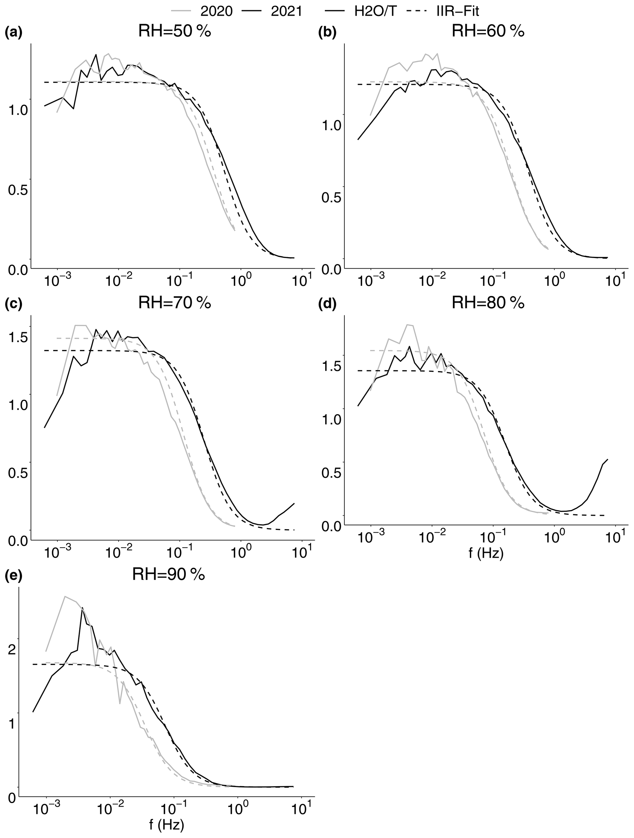
Figure A1 The ratio of ensemble-averaged normalized $\frac{{\mathrm{H}}_{\mathrm{2}}\mathrm{O}}{T}$ spectra (solid line) of the CON-EC versus the natural frequency. Additionally, the linear IIR fit obtained with EddyPro (dashed line) is shown, which represents the transfer function for the high-frequency corrections used for the CON-EC H₂O flux calculations. The ratios and transfer functions are shown for the 2020 (grey) and 2021 (black) grassland campaigns and are presented in five RH-class bins obtained with EddyPro.