Deriving the hygroscopicity of ambient particles using low-cost optical particle counters

This study investigates the chemical composition and physical properties of aerosols, which play a crucial role in influencing human health, cloud physics, and local climate. Our focus centers on the hygroscopicity of ambient aerosols, a key property reflecting the ability to take up moisture from the atmosphere and serve as cloud condensation nuclei. Employing home-built air quality box (AQB) systems equipped with low-cost sensors, we assess the ambient variability of particulate matter (PM) concentrations to determine PM hygroscopicity. The AQB systems effectively captured meteorological parameters and most pollutant concentrations, showing high correlations with data from the Taiwan Environmental Protection Administration (TW-EPA). With the application of κ-Köhler equation and certain assumptions, AQB-monitored PM concentrations are converted to dry particle mass concentration, providing optical particle counter sensitivity correction and resulting in improved correlation with TW-EPA data. The derived single hygroscopicity parameters (κ) range from 0.15 to 0.29 for integrated fine particles (PM_2.5) and 0.05 to 0.13 for coarse particles (PM_2.5−10), consistent with results of ionic chromatography analysis from a previous winter campaign nearby. Moreover, the analysis of PM₁₀ division into PM_2.5 and PM_2.5−10, considering composition heterogeneity, provided improved dry PM₁₀ concentration as the sensitivity coefficients for PM_2.5−10 were notably higher than for PM_2.5. Our methodology provides a comprehensive approach to assess ambient aerosol hygroscopicity, with significant implications for atmospheric modeling, particularly in evaluating aerosol efficiency as cloud condensation nuclei and in radiative transfer calculations. Overall, the AQB systems proved to be effective in monitoring air quality and deriving key aerosol properties, contributing valuable insights into atmospheric science.

1 Introduction

In an era of increased industrialization, individuals face growing exposure to poor air quality, elevating the risks of cardiovascular and respiratory diseases (Chen et al., 2017; Brook et al., 2010; Heus et al., 2010). Within the realm of air pollutants, atmospheric aerosols emerge as critical components, playing a vital role in Earth's climate system. They influence radiative balance, cloud formation, and precipitation patterns, while significantly impacting human health, visibility, and ecosystems (Pöschl et al., 2010; Wu et al., 2010; Brook et al., 2010; Hamanaka and Mutlu, 2018). Their ability to scatter and absorb solar radiation, coupled with their role as cloud condensation nuclei (CCNs), emphasizes their significance in shaping both climate dynamics and air quality (Andreae and Rosenfeld, 2008; Rosenfeld et al., 2014; Lohmann and Feichter, 2005). However, understanding the complex interplay between aerosols and these processes requires the physical and chemical properties of aerosols, including hygroscopicity. The hygroscopic growth of aerosol particles, indicating their ability to take up moisture from the ambient air, alters their size distribution, mass, optical properties, and CCN activity, thereby impacting climate dynamics and air quality (Petters and Kreidenweis, 2007). The traditional methods such as hygroscopic tandem differential mobility analyzers and cloud condensation nuclei counters (Chan and Chan, 2005; Hung et al., 2016; Bian et al., 2014) have provided valuable insights into the hygroscopic properties of various aerosol types. However, their complexity and cost often limit their applicability for extensive, long-term measurements.

Over the past decade, the rise in popularity of low-cost optical particle counters (OPCs) can be attributed to their simplicity, portability, and affordability (Sá et al., 2022; Crilley et al., 2018; Samad et al., 2021). OPCs provide real-time data on particle size distributions and mass concentrations with high temporal resolution for monitoring ambient particles. However, challenges arise in ensuring the accuracy of OPCs, necessitating additional constraints or calibrations for optimal performance. The measurement principle of OPCs relies on the dependence of Mie scattering on particle size, yet this dependence is non-monotonic across all sizes. Additionally, particle composition influences light scattering, leading to varying scattering efficiencies (Kaliszewski et al., 2020; Formenti et al., 2021). Variations in particle density directly affect the mass concentration derived from the monitored number size concentration (Hagan and Kroll, 2020; Dacunto et al., 2015). A particularly challenging issue involves the removal of liquid water from ambient particles. Several studies have attempted to derive the dry mass concentration of ambient particles using OPC, employing calibration methods linked to the hygroscopic growth factor (HGF) under controlled relative humidity (RH) conditions. Notably, Crilley et al. (2018) improved OPC mass concentration correction by applying the derived hygroscopicity (κ) values of 0.38–0.41 and 0.48–0.51 for PM_2.5 and PM₁₀, respectively, achieving a 33 % improvement. Similarly, Di Antonio et al. (2018) and Venkatraman Jagatha et al. (2021) elevated calibration from a moderate to a high correlation by assuming a constant κ of 0.40. Furthermore, the chemical composition and physical properties of aerosols exhibit high temporal–spatial variation, making the analysis and correction of observational data from a physical perspective crucial. The widespread adoption of low-cost sensors, attributed to their affordability, enables more extensive use as users find them more accessible (Castell et al., 2017). This increased utilization enhances spatial resolution in environmental monitoring, deepening our understanding of pollution evolution. However, it is essential to emphasize that regular maintenance and calibration are necessary for accurate results (Concas et al., 2021; Sá et al., 2022).

In this study, we evaluate the performance of our home-built monitoring system, air quality box (AQB), through a comprehensive analysis and calibration by co-locating the two AQB systems with the Taiwan Environmental Protection Administration (TW-EPA) station. Our primary focus is on OPCs, for which we employed a physical model to elucidate the hygroscopic characteristics of ambient particles during the determination of dry particle mass concentrations for integrated fine particles (PM_2.5, D_p≤2.5 µm) and coarse particles (PM_2.5−10, 2.5 µm <D_p ≤ 10 µm). Additionally, we discuss various factors contributing to errors in hygroscopicity estimates, aiming to gain valuable insights into using low-cost sensors for extensive and prolonged monitoring applications.

2 Methodology

2.1 Air quality box (AQB) system

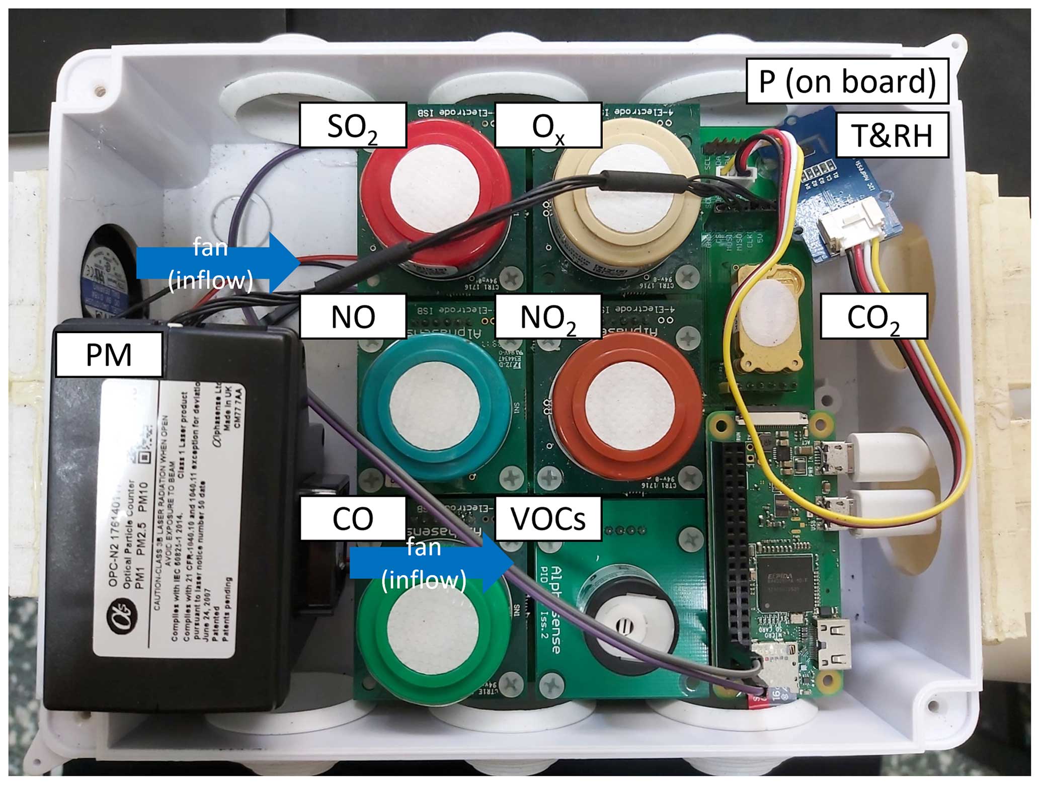
Two home-built AQB systems (AQB no. 1 and AQB no. 2) consist of multiple sensors that monitor meteorological parameters such as temperature (T), relative humidity (RH), and pressure (P), as well as gaseous species and particulate matter (PM) with a temporal resolution of seconds as shown in Fig. 1 with sensor information summarized in Table S1. The gas sensors include five Alphasense amperometric B4 series sensors that measure CO, NO, NO₂, O_x (O₃+ NO₂), and SO₂; a photo-ionization detector (PID-AH2, Alphasense) monitoring volatile organic compounds; and a non-dispersive infrared CO₂ sensor from Amphenol Advanced Sensors (T6713-5K). The PID sensor, equipped with a krypton lamp providing a photon energy of about 10.6 eV, cannot detect methane, which has a higher ionization potential of ∼ 13.7 eV (Glockler, 1926). Therefore, the data of non-methane hydrocarbons (NMHC) from TW-EPA are more comparable to PID data in our analysis. The PM sensor (OPC-N2, Alphasense), an optical particle counter, monitors the number size distribution between 0.38 and 17 µm, divided into 16 bins based on Mie scattering, with a sampling flow rate of ∼ 4 mL s⁻¹ and a refractive index of 1.5+0 i. In addition, the mass concentration of PM₁, PM_2.5, and PM₁₀ could be calculated from the number size distribution, assuming a particle density of 1.65 g cm⁻³. These sensors were controlled by a small single-board computer, Raspberry Pi Zero W, at a time resolution of 3 s with data stored in a microSD card and uploaded to cloud storage via 4G LTE. The entire system is housed in a remodeled enclosure with a dimension of 25 cm × 16 cm × 8 cm (L × D × H) and has well-ventilated openings for sampling and exhaust. The sampling flow rate is primarily controlled by an installed fan at ∼ 5.6 L min⁻¹, corresponding to a residence time of approximately 34 s in the box. This configuration allows the system to effectively monitor ambient air quality independently without the need of additional inlets.

Figure 1 The design of the AQB system.

2.2 Calibration campaign and reference data

The calibration of AQB sensors was carried out by co-locating them with the TW-EPA Nanzi station (Fig. S1) in Kaohsiung, Taiwan (22°44^′12^′′ N, 120°19^′42^′′ E) from 4 to 19 February 2021. Nanzi station is situated on the roof of a 15 m high building in a well-ventilated environment. The primary gaseous components, dry PM_2.5 and PM₁₀ concentrations, and basic meteorological parameters are continuously monitored using standard instruments, as summarized in Table S1. For electrochemical sensors in AQB, the performance can be influenced by environmental parameters such as temperature, relative humidity, and other chemical species that have high cross sensitivity (Concas et al., 2021; Karagulian et al., 2019; Mead et al., 2013). Therefore, in this study, a linear regression with a multivariate function of voltage and the environmental temperature was applied to retrieve concentrations for gas species. For PM, the reported values by beta attenuation mass monitor (BAM) in the TW-EPA station reflect the dry-state PM concentration by controlling the measurement at RH less than 50 % (i.e., a heating device applied to reduce the sampling flow to 35 % water saturation when the ambient RH is > 50 %). On the contrary, the optical particle counter (OPC) in AQB directly monitors ambient PM concentration. The difference between BAM and OPC data reflects the amount of liquid water content in ambient conditions. A simple linear regression between them might not completely reveal the influence of hygroscopicity. Therefore, the κ-Köhler equation (Petters and Kreidenweis, 2007) was applied to derive the κ as discussed in the following section.

2.3 Sensitivity coefficients of OPCs and particle hygroscopicity

To bridge the PM concentration gap between BAM and OPC, the sensitivity correction of OPC and the conversion of ambient particles to dry particles are required. The sensitivity coefficient (α) was evaluated as the mass concentration ratio of BAM and OPC data at low RH (≤50 %) having limited water content, as follows:

$$\begin{array}{}\text{(1)}& \mathit{\alpha }={\displaystyle \frac{M_{\mathrm{BAM}}}{M_{\mathrm{OPC}}}},\end{array}$$

where M_BAM andM_OPC are PM mass concentrations (µg m⁻³) measured by BAM and OPC, respectively. RH ≤ 50 % was applied as the threshold criteria for data selection to determine α, as the mass concentration of ambient particles might have significant water uptake at higher RH. The statistical distribution of M_BAM to M_OPC ratios at RH ≤ 50 % was analyzed to assign α as the mean value ± 0.5σ (σ: standard deviation) to prevent high-concentration data points from dominating the statistical result.

The particle size growth with the water saturation ratio (S) for a given κ can be evaluated using κ-Köhler equation as follows (Petters and Kreidenweis, 2007):

$$\begin{array}{}\text{(2)}& S={\displaystyle \frac{D_{\mathrm{amb}}^{\mathrm{3}}-D_{\mathrm{d}}^{\mathrm{3}}}{D_{\mathrm{amb}}^{\mathrm{3}}-D_{\mathrm{d}}^{\mathrm{3}}\left(\mathrm{1}-\mathit{\kappa }\right)}}\exp \left({\displaystyle \frac{\mathrm{4}{\mathit{\sigma }}_{s/a}{M}_{\mathrm{w}}}{RT{\mathit{\rho }}_{\mathrm{w}}{D}_{\mathrm{amb}}}}\right),\end{array}$$

where D_amb and D_d are the diameters (m) of the ambient and dry particulate matter, respectively; ${\mathit{\sigma }}_{s/a}$ is the surface tension of the particle (J m⁻²); M_w is the molecular weight of water (g mol⁻¹); R is the gas constant (J mol⁻¹ K⁻¹); T is the temperature; and ρ_w is the density of liquid water (1.0 g cm⁻³). The first term is the solute effect, while the second is the Kelvin effect. As the mass is dominated by the larger particles, the Kelvin effect in Eq. (2) is assumed to be negligible for simplification. The derived dry mass concentration (M_d,derived) from the measured ambient particles from OPC data can be expressed as follows (Pope et al., 2010; Crilley et al., 2018):

$$\begin{array}{}\text{(3)}& M_{\mathrm{d},\mathrm{derived}}=(\mathit{\alpha }\times M_{\mathrm{OPC}})\times {\left[\left({\displaystyle \frac{S\mathit{\kappa }}{\mathrm{1}-S}}\right)\times {\displaystyle \frac{{\mathit{\rho }}_{\mathrm{w}}}{{\mathit{\rho }}_{\mathrm{d}}}}+\mathrm{1}\right]}^{-\mathrm{1}},\end{array}$$

where ρ_d is the density of dry aerosol particles and is assumed to be 1.20 g cm⁻³ in this study. With the determined α values (Eq. 1), κ can be derived from the data points of aqueous particles at RH above 70 %, and the deliquescence RH (DRH) can be verified using ion chromatography (IC) analyzed composition with the Extended Aerosol Inorganics Model (E-AIM) model. The mean absolute percentage error (MAPE) parameter between M_d,derived and M_BAM was used to assess the appropriate κ value as follows:

$$\begin{array}{}\text{(4)}& \mathrm{MAPE}={\displaystyle \frac{{\sum }_{i=\mathrm{1}}^n\frac{\left|M_{\mathrm{d},\mathrm{derived},i}-M_{\mathrm{BAM},i}\right|}{M_{\mathrm{BAM},i}}}{n}}\times \mathrm{100}\mathit{\%},\end{array}$$

where n is the total number of data points. With the restricted range of α, κ can be derived under the minimum MAPE. The detailed process description for κ derivation is provided in the Supplement. Due to the heterogeneity between particles, PM₁₀ was divided into integrated fine particles (D_p≤2.5 µm) and coarse particles (2.5 µm <D_p≤10 µm) to evaluate the individual sensitivity coefficient and hygroscopicity.

2.4 Composition analysis

Hygroscopicity can also be determined using the volume fraction of the major components. Based on an earlier field campaign, the ion chromatography (IC) method was applied to quantify water-soluble components for samples (both PM_2.5 and PM₁₀) collected at Fooyin University (22°36^′09.8^′′ N, 120°23^′23.1^′′ E) in Kaohsiung from 15 to 28 January 2013. Ambient aerosol samples were collected using a pair of dichotomous aerosol samplers (model RP-2025, R&P Co., Inc., Albany, New York) to collect integrated fine and coarse particles on Teflon filters with sampling flow rates of 15.0 and 16.7 L min⁻¹, respectively. The samples were categorized into daytime and nighttime. Daytime samples were collected from 08:00 to 20:00 LT, and nighttime samples were collected from 20:00 to 08:00 LT the next day. The samplers were equipped with Teflon filters deployed for the measurement of water-soluble ions (Na⁺, Mg²⁺, K⁺, Ca²⁺, NH${}_{\mathrm{4}}^{+}$, Cl⁻, SO${}_{\mathrm{4}}^{\mathrm{2}-}$, and NO${}_{\mathrm{3}}^{-}$) via ion chromatography (model ICS-1000, Dionex). More information on the chemical analysis method can be found in Salvador and Chou (2014).

To derive the hygroscopicity from samplings, the ions from IC analysis were converted to chemical components via the following sequence: ammonium sulfate, ammonium bisulfate, ammonium nitrate (when there is residual ammonium), sodium nitrate, and sodium chloride. With the assumption of the hygroscopicity of insoluble components as zero and negligible residual ion contribution (less than 5 % of total mass), the overall hygroscopicity can be derived by the volume fraction (ε_i) weighted hygroscopicity from individual soluble component (i species) as follows:

$$\begin{array}{}\text{(5)}& \mathit{\kappa }={\sum }_i{\mathit{\epsilon }}_i{\mathit{\kappa }}_i={\sum }_i{\displaystyle \frac{v_i}{v_{\mathrm{total}}}}{\mathit{\kappa }}_i,\end{array}$$

where κ_i is the hygroscopicity of i species, v_total is the volume of particles, and v_i is the volume of i species. The conversion of particle mass to volume is based on a density of 1.20 g cm⁻³. The applied hygroscopicity, molecular weight, and density for the related chemical species are summarized in Table S2. With the assumption that these ions dissolve completely in the aqueous phase, which represents the maximum estimation, the hygroscopicity contributed by the residual ions were found to be approximately up to 1.8 % and 6.4 % of the overall κ value for integrated fine particles (PM_2.5) and coarse particles (PM_2.5−10), respectively. Given their limited impact on the hygroscopic behavior of the particles, the contribution of the residual ions was not taken into account in the calculation. Additionally, other PM_2.5 IC data for samples collected at the National Kaohsiung University of Science and Technology (22°46^′22.4^′′ N, 120°24^′03.4^′′ E) in Kaohsiung for the period of 8–18 December 2021 samples were also applied for further comparison (no PM₁₀ collection for that campaign). We opted for the 2013 dataset for more discussion due to its comprehensive analysis encompassing both PM_2.5 and PM_2.5−10. Furthermore, the composition data obtained from IC analysis was applied to E-AIM Model III (for systems containing H⁺, NH${}_{\mathrm{4}}^{+}$, Na⁺, SO${}_{\mathrm{4}}^{\mathrm{2}}$, NO${}_{\mathrm{3}}^{-}$, Cl⁻, and H₂O) to evaluate the characteristics of volume variation as a function of RH in the range of 30 % to 90 % (Clegg et al., 1998). The partitioning of selected trace gases (HNO₃, HCl, NH₃, and H₂SO₄) into the vapor phase was disabled to keep a consistent quantity of applied chemical species in the particle phase. The growth factor, $V_{\mathrm{amb}}/V_{\mathrm{d}}$, above DRH, was applied to retrieve the κ value using Eq. (2) but without the Kelvin effect term (Luo et al., 2020). Both the individual sample concentrations and the overall averaged composition conditions were analyzed to evaluate the hygroscopic behavior of the particles.

3 Results and discussion

3.1 Performance of AQB systems

Figure 2 shows the time series of the meteorological parameters and pollutant concentrations between calibrated AQB and TW-EPA data from 14 to 17 February 2021. T, RH, CO, and O_x showed a good correlation with r>0.9, while NO, NO₂, PM_2.5, and PM₁₀ had a moderate correlation (r≥0.48). The high correlation (r=0.976) for CO (with a lifetime of ∼ 2 months) indicates a similar air parcel sampled by both AQB and the instrumentation in TW-EPA. The PID sensor had consistent peaks with high NMHC concentrations and could not reveal temporal variation at low concentrations, resulting in a low correlation. Overall, the AQB system performs well in capturing the ambient variability of pollutants stated above. The low correlation of SO₂ was due to the cross sensitivity of this SO₂ sensor, which was highly sensitive to O₃ and NO₂ (about −120 % reported in the technical specifications of Alphasense). O₃ and NO₂ generally have higher concentrations than SO₂ and cause a significant contribution to the response of the SO₂ sensor. However, if high-SO₂-concentration events occur, the SO₂ sensor might reflect the variation in SO₂ concentration. The PM concentration shown in Fig. 2 was calibrated using a simple linear regression, which roughly reflects the trend of mass concentration but shows more significant deviations at higher RH due to more water uptake in particles, as discussed in Sect. 3.2. Most gas species showed a high correlation (r≥0.95) between different AQB systems except for NMHC (r=0.675) as summarized in Table S3. Further results and discussions focus on the PM analysis using AQB no. 1, which has a more consistent sampling rate during the observation period, unless stated otherwise.

Figure 2 The temporal profiles of calibrated AQB data (red lines) and the TW-EPA measurement (gray lines) for (a) temperature, (b) relative humidity, (c) CO, (d) NO, (e) NO₂, (f) O_x (≡ NO₂+ O₃), (g) non-methane hydrocarbon, (h) SO₂, (i) PM_2.5, and (j) PM₁₀ during the period of 14–17 February 2021 (4 of 16 d in period). All the species were calibrated using linear regression.

3.2 Comparison between OPC and BAM data

3.2.1 Sensitivity coefficient of OPC

Figure 3a and c show the scatter distribution of the mass concentrations between OPC (with no calibration) and BAM data for PM_2.5 and PM₁₀, respectively. Overall, the PM mass concentrations measured by OPC have a similar trend to those measured by BAM but exhibit some variability. The results reveal an apparent influence of ambient RH, indicating the contribution of water content. The red-shaded area represents a regression line with a slope corresponding to the inverse of the α derived from data points at ambient RH ≤ 50 % (17 out of 356 points, 5 %). The notable deviation of the red-shaded area from the 1:1 line towards the right side indicates the requirement of α>1 corrections, contributed by the different measurement principles and calibration techniques, which may result from the assumed particle density and refractive index (RI) (dust, density: 1.65 g cm⁻³; RI: 1.5+0 i). The estimated α values, as summarized in Table 1, are higher for PM₁₀ than for PM_2.5, i.e., 2.02 ± 0.34 vs. 1.26 ± 0.16, and are reasonably conclusive as tested with more data points selected at higher RH thresholds (Fig. S2). The α difference between PM_2.5 and PM₁₀ might be attributed to the complex composition of ambient particles, which differs from the samples used for instrument calibration, as well as possible sensitivity variations in OPC over time. With sensitivity calibration, the performance at ambient RH ≤ 50 % exhibits a strong correlation with MAPE at 12.8 % and 18.5 % as well as a root mean squared error (RMSE) at 3.7 µg m⁻³ and 10.3 µg m⁻³ for PM_2.5 and PM₁₀, respectively, as summarized in Table 2 excluding the two significant outliers (shown as hollow circles in Fig. 3). The results confirm the effectiveness of OPCs in capturing PM concentrations after proper calibration, consistent with other real-time outdoor field studies, reporting R² ranging from 0.34 to 0.97, RMSE ranging from 0.52 to 12.3 µg m⁻³, and MAPE about 22 % (Gillooly et al., 2019; Demanega et al., 2021; Sá et al., 2022; Crilley et al., 2018). Additionally, the OPC sampling flow rate has an impact on measurement performance. AQB no. 1 maintained a steady rate at 3.6 ± 0.2 L min⁻¹, whereas AQB no. 2 exhibits two distinct periods with sampling flow rates of 3.6–4.2 L min⁻¹ for the first period and 3.2–3.6 L min⁻¹ for the second period. The distinctive sampling flow rates result in a non-linear change in α, suggesting the need to separate the data into two parts to estimate the individual α (Fig. S3).

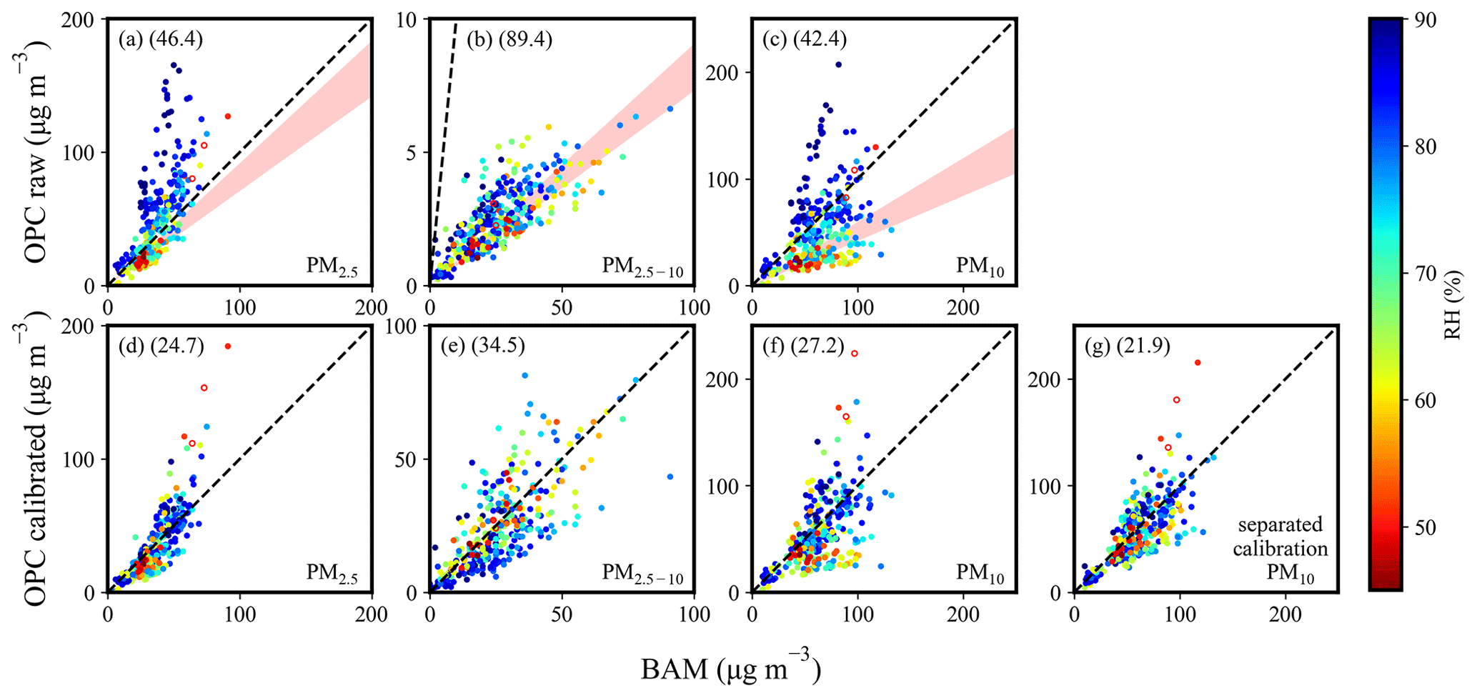
Figure 3 The correlation of mass concentration between BAM and OPC in AQB no. 1 (raw data or calibrated data): (a, d) PM_2.5, (b, e) PM_2.5−10, (c, f) PM₁₀, and (f) separated calibration PM₁₀. Panels (a)–(c) are the raw data, while panels (d)–(g) are the calibrated data. The marker color corresponds to relative humidity. The hollow points are the two significant outliers under conditions of RH ≤ 50 %. The shaded region represents the data associated with the sensitivity coefficient (α). The value in parentheses is the MAPE in percentage.

Table 1 The sensitivity coefficients and the hygroscopicity for PM_2.5, PM₁₀, and PM_2.5−10.

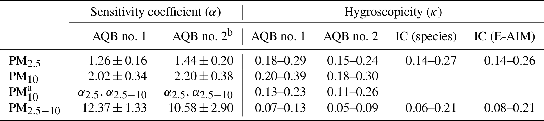
^a The hygroscopicity derived using different sensitivity coefficients for different size ranges. α_2.5 and α_2.5−10 are sensitivity coefficients for PM_2.5 and PM_2.5−10, respectively. More details are provided in the description of the Supplement. ^b The sensitivity of AQB no. 2 presents the value in the period of sampling flow rates at 3.6–4.2 L min⁻¹.

Table 2 Performance metrics of different calibration methods for PM_2.5, PM_2.5−10, and PM₁₀.

^a Only for data points at RH ≤ 50 %. The value in parentheses is the performance result without two significant outliers shown in Fig. 3. ^b Coefficient of determination (R²) is calculated as the proportion of variation in the calibrated dry mass concentration. ^c The combination of calibrated data from PM_2.5 all data (κ=0.29) and PM_2.5−10 all data (κ=0.09).

3.2.2 Hygroscopicity derivation

With the derived α, the hygroscopicities were retrieved using Eq. (3), resulting in κ ranging from 0.18 to 0.29 for PM_2.5 and 0.20 to 0.39 for PM₁₀ during the studied period, as summarized in Table 1. Figure 3d and f show the scatter distribution of the derived dry concentration vs. BAM concentration for PM_2.5 and PM₁₀, respectively. The results from the two OPCs exhibit slight differences but are consistent overall. Considering both the sensitivity coefficient and hygroscopicity, the performance of OPC in deriving dry PM concentration is significantly improved with lower MAPE, RMSE, and higher R² than the results obtained using only the sensitivity coefficient, as summarized in Table 2. With a similar methodology, Crilley et al. (2018) applied the κ-Köhler equation to compare measured data between OPC-N2 and tapered element oscillating microbalance (TEOM) and derived the κ ranging from 0.38 to 0.41 and 0.48 to 0.51 for PM_2.5 and PM₁₀, respectively, which is within the range for Europe (i.e., 0.36 ± 0.16) (Pringle et al., 2010).

Due to the heterogeneity of composition among different sizes, PM₁₀ can be divided into PM_2.5 and PM_2.5−10 for further analysis. The estimated α value for PM_2.5−10, as summarized in Table 1, is approximately 1 order of magnitude higher than that for PM_2.5. The lower κ for PM_2.5−10 might suggest a significant contribution from dust or other less hygroscopic species, consistent with the IC analyses in Table 3 and discussed further in Sect. 3.3. With the retrieved α and κ for PM_2.5 and PM_2.5−10, Fig. 3e shows the scatter distribution between the derived dry PM_2.5−10 from OPC and BAM data, exhibiting a MAPE of 31.8 %, which is more significant than the 24.8 % for PM_2.5. The higher MAPE might result from the low particle number concentration in the coarse mode, with only about 0.01 to 0.1 particles per bin per cubic centimeter in the size range of 3.0 to 10.0 µm. The results are consistent with the findings of Kaliszewski et al. (2020), which showed that the correlation between OPC-N3 (a newer version of OPC-N2) and AeroTrak 8220 (TSI Inc., Shoreview, MN, USA) measurement data decreases with particle size, from 0.3–0.5 µm (r=0.99) to 5–10 µm (r=0.74). The dry PM₁₀ derived from OPC through the divided PM_2.5 and PM_2.5−10 analysis demonstrates better consistency with the reported BAM data than the direct calibration method. This is evidenced by a lower MAPE in Fig. 3g (18.2 %) compared to Fig. 3f (29.2 %) and a significant improvement than the simple linear regression method, which has a higher MAPE at 62.5 % (Table 2). Moreover, the derived κ for PM₁₀ with the size-dependent sensitivity coefficient correction ranges from 0.13 to 0.23 (Table 1). This value falls between those for PM_2.5 and PM_2.5−10 and is more reasonable compared to κ derived with a fixed sensitivity coefficient (κ=0.20–0.39, higher than those for PM_2.5 and PM_2.5−10). The results substantiate the importance of considering composition heterogeneity among particle sizes for accurate dry PM derivation.

Table 3 The total mass concentration, major water-soluble composition, and concentration (mean value and standard deviation in µg m⁻³) of winter PM_2.5 and PM_2.5−10 in Kaohsiung by ion chromatography (“Others” represents the insoluble composition).

3.3 Hygroscopicity derivation using IC data

3.3.1 Composition analysis

The major soluble composition and concentrations obtained from the IC analysis are summarized in Table 3. The mean concentrations of PM_2.5 and PM_2.5−10 are 67 ± 19 and 36 ± 7 µg m⁻³, respectively. The determined soluble composition of PM_2.5 constitutes approximately 53 % of the mass fraction and is predominantly composed of NH${}_{\mathrm{4}}^{+}$, SO${}_{\mathrm{4}}^{\mathrm{2}-}$, and NO${}_{\mathrm{3}}^{-}$, which are formed through chemical reactions involving industrial and agricultural emissions. In contrast, ∼ 30 % of PM_2.5−10 is soluble components, including NO${}_{\mathrm{3}}^{-}$, SO${}_{\mathrm{4}}^{\mathrm{2}-}$, Na⁺, Cl⁻, NH${}_{\mathrm{4}}^{+}$, and some alkaline earth metal ions (Ca²⁺ and Mg²⁺), with a more significant proportion being insoluble components (∼ 70 %), likely attributed to dust, metallic elements, and unanalyzed organic components. The higher portion of sea salt (Na⁺ and Cl⁻) in PM_2.5−10 than in PM_2.5 is likely transported by the sea breeze during the daytime, while the increased fractions of Ca²⁺ and Mg²⁺ might correspond to sand or dust particles (Li et al., 2022).

The temporal variation of derived κ, based on the IC soluble composition analysis, ranges from 0.14 to 0.26 for PM_2.5 and 0.06 to 0.21 for PM_2.5−10, as shown in Fig. S4a and summarized in Table 1. A similar analysis for the winter of 2021 showed a similar κ range for PM_2.5, as illustrated in Fig. S5. This consistency across distinct study periods indicates typical winter hygroscopic characteristics for ambient PM_2.5 in Kaohsiung, applicable for further discussion with the OPC data. For PM_2.5−10, the more significant variability in κ compared to PM_2.5 can be attributed to substantial fluctuations of soluble composition in coarse particles, primarily driven by significant quantities of thenardite (Na₂SO₄) and halite (NaCl) (Tang et al., 2019). Due to the dominance of the northeast monsoon wind during the filter sampling period, the influence of the sea–land breeze was too relatively weak to cause apparent diurnal variation in κ.

The κ values derived from IC analysis reflect the temporal variation, while those from OPC analysis indicate the overall physical properties of ambient aerosols for the studied period. Factors such as spatial and temporal variations in aerosols, different campaign years and locations (∼ 20 km apart, as shown in Fig. S1), and technique uncertainties, such as ammonia and nitrate sampling evaporation during filter sampling (Hering and Cass, 1999; Chen et al., 2021), as well as OPC detection uncertainties and assumption required for calculation, can influence comparisons. However, the results (i.e., ∼ 0.22 (OPC) vs. 0.14–0.27 (IC) for PM_2.5 and ∼ 0.09 (OPC) vs. 0.06–0.21 (IC) for PM_2.5−10) summarized in Table 1 and Fig. 4a suggest that the derived κ values from OPC data likely reflect the mean hygroscopicity for the integrated fine and coarse particles during winter in Kaohsiung.

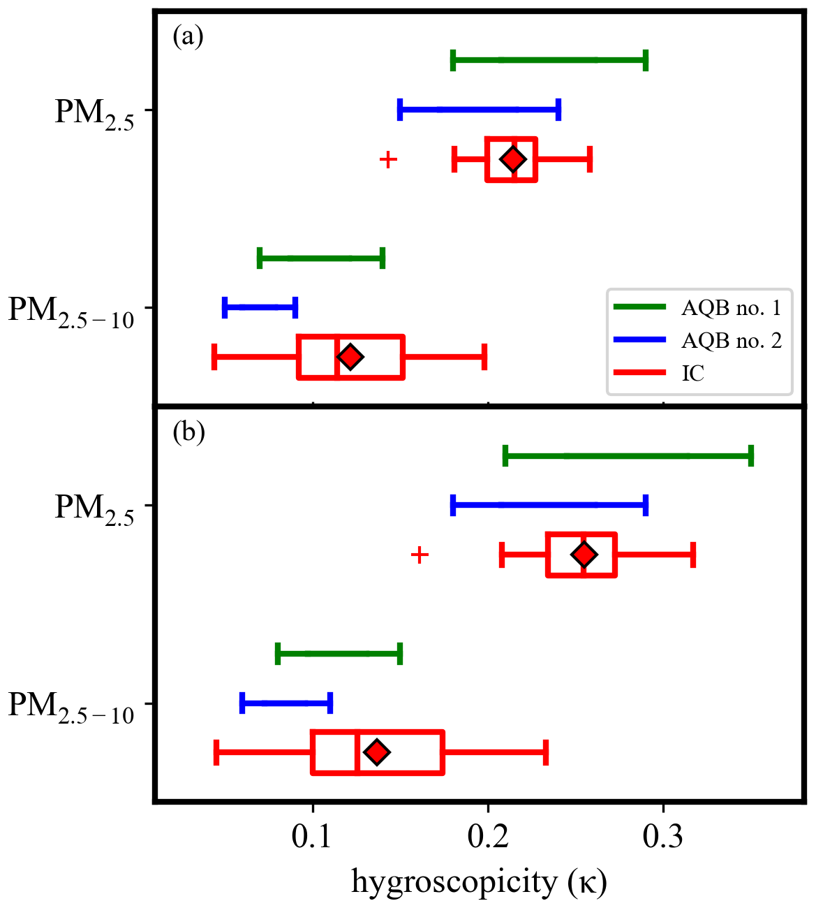
Figure 4 The hygroscopicities of PM_2.5 and PM_2.5−10 derived based on data from OPCs and ion chromatography with the assumption particle density of (a) 1.2 g cm⁻³ and (b) 1.42 ± 0.03 and 1.34 ± 0.07 g cm⁻³ for PM_2.5 and PM_2.5−10, respectively, based on analyzed composition. The average value is shown as a red diamond.

3.3.2 E-AIM analysis

With the measured composition, the hygroscopicity can be derived from the growth pattern. The particle growth might follow the κ-Köhler equation (Eq. 2) when all soluble species are fully dissolved, typically occurring above the DRH. Using the averaged soluble composition determined from the IC analysis, HGF as a function of RH calculated using E-AIM is shown in Fig. 5. For PM_2.5, partial deliquescence initiates at 60 % RH with some residual solid components such as ((NH₄)₂SO₄ and 2NH₄NO₃ ⋅ (NH₄)₂SO₄). Complete dissolution occurs at RH ∼ 72 %. In the case of PM_2.5−10, water uptake begins at 42 % RH, leaving a residual solid composed of 3NH₄NO₃(NH₄)₂SO₄, NH₄Cl, and NaNO₃ ⋅ Na₂SO₄ ⋅ H₂O until reaching 68 % RH. The daily DRH happens at 71.3 ± 4.9 % and 67.1 ± 3.4 % for PM_2.5 and PM_2.5−10, respectively, as shown in Fig. S4b and c. In the OPC data analysis, an RH threshold of ≤ 50 % was applied to determine the sensitivity. At this threshold, PM_2.5 particles have not yet deliquesced, and PM_2.5−10 shows minimal volume growth, indicating the applicability of the selected RH threshold for sensitivity calculation. A DRH threshold of 70 % was applied to ensure sufficient data points for κ calculation but slightly lower than the DRH of PM_2.5.

Figure 5 The volume ratio of a given soluble composition as a function of RH under thermodynamic equilibrium calculated using E-AIM at 298.15 K (composition is the averaged IC data with a molarity ratio of Na⁺ : NH${}_{\mathrm{4}}^{+}$ : Cl⁻ : SO${}_{\mathrm{4}}^{\mathrm{2}-}$:NO${}_{\mathrm{3}}^{-}$ as $\mathrm{7}:\mathrm{229}:\mathrm{0}:\mathrm{71}:\mathrm{94}$ for PM_2.5 and $\mathrm{65}:\mathrm{59}:\mathrm{16}:\mathrm{19}:\mathrm{70}$ for PM_2.5−10).

To assess the potential bias associated with the selected DRH threshold, Fig. S6 shows the HGF of mean soluble composition as a function of RH estimated using E-AIM. With Eq. (2) (without the Kelvin effect term) and the assumption of volume additivity between the particle and the water taken up, κ values derived using 70 % and 75 % thresholds show less than 1 % difference for PM_2.5 and PM_2.5−10 compositions but 13 % and 6 % less than that estimated from the composition calculation (Eq. 5) for PM_2.5 and PM_2.5−10, respectively. As the selected DRH threshold decreases, the derived κ decreases slightly due to the interference of adding data points with incompletely dissociated composition to the fitting analysis. However, the temporal composition variation in the applied OPC dataset (∼ 16 d of observation) might lead to a higher variation (Fig. S7), making the κ deviation due to the applied DRH threshold appear negligible in this study. Furthermore, the lower derived κ for E-AIM compared to the composition estimation is likely due to the applied individual κ values in composition estimation being based on CCN activation measurement, which was reported to be 10 % to 17 % higher than that derived from the growth factor analysis (Petters and Kreidenweis, 2007). During the particle growth process, the partial dissociation leads to the RH-dependent van't Hoff factor, as noted by Petters and Kreidenweis (2007). Similar findings were reported by Kreidenweis et al. (2008) regarding the differences in derived water contents between the κ-Köhler equation and E-AIM to be within ± 20 % under the condition of approximately 85 % RH, which might cause differences for κ evaluation. Overall, the differences in derived κ among methods are primarily due to the given hygroscopicity of chemical species, likely due to the fixed van't Hoff factor and the assumptions of volume additivity in the κ-Köhler equation.

3.4 Sensitivity of assumed parameters on derived hygroscopicity

For simplicity, κ was derived from OPC and BAM data without considering the Kelvin effect and under an assumed particle density. Neglecting the Kelvin effect may result in minor differences for particles larger than 100 nm under sub-saturated conditions (Pope et al., 2010; Topping et al., 2005; Crilley et al., 2018). To confirm the appropriateness, we assessed biases for particles at 0.1 and 1 µm without considering the Kelvin effect, as shown in Fig. S8. For particles with a κ value of 0.3 under RH ranging from 70 % to 95 %, the deviation of κ due to neglecting the Kelvin effect is −10 % for 0.1 µm particles and −1 % for 1 µm particles, decreasing with particle diameter. The particle diameter is overestimated under the same RH conditions because the positive Kelvin effect is ignored. To compensate for the deficiency in saturation, the balanced particle diameter needs to be larger with a more significant solute effect. However, the average mass-weighted mean diameter for PM_2.5 is about 1.3 µm. Therefore, neglecting the Kelvin effect in our analysis has limited influence on the derived κ.

Furthermore, the derived κ from OPC data (using Eq. 3) and IC data (using Eq. 5) are notably influenced by the assumed particle density. Assuming that the undetermined composition mainly consists of secondary organic species with a density of 1.2 g cm⁻³, within the reported densities ranging from 0.9 to 1.6 g cm⁻³ depending on the formation process (Malloy et al., 2009; Kostenidou et al., 2007; Zelenyuk et al., 2008), along with the properties of analyzed soluble chemical species summarized in Table S2, the calculated densities are 1.42 ± 0.03 and 1.34 ± 0.05 g cm⁻³ for PM_2.5 and PM_2.5−10, respectively (Fig. S9). These calculated densities are about 15 % and 10 % higher than the assumed fixed density (1.2 g cm⁻³) for PM_2.5 and PM_2.5−10, respectively. Consequently, the derived κ from OPC data increases by approximately 17 % for PM_2.5 and 9 % for PM_2.5−10, while the derived κ from IC data is proportional to density (i.e., 15 % and 10 % for PM_2.5 and PM_2.5−10, respectively) as shown in Fig. 4b. This influence is particularly noticeable for components with a high portion of higher-density species, such as black carbon (a non-hygroscopic species with κ∼ 0) having a high density of about 1.8 g cm⁻³ (Park et al., 2004; Shiraiwa et al., 2008). Despite the potential uncertainties associated with particle density, the derived κ exhibits consistency between the OPC and IC analyses.

4 Conclusions

In this study, we evaluated the performances of home-built air quality box (AQB) systems equipped with low-cost sensors and focused on the ambient variability of particulate matter (PM) concentrations to derive the hygroscopicity of PM and the conversion to dry particle concentrations. The AQB systems revealed their effectiveness in capturing meteorological parameters and most pollutant concentrations with high correlations (r≥0.96) for temperature, relative humidity, CO, and O_x (O₃+ NO₂) and moderate correlations (r≥0.48) for NO_x and PM, as compared to TW-EPA data. In the PM analysis, PM₁₀ was divided into PM_2.5 and PM_2.5−10 to account for compositional heterogeneity among different particle sizes. Comparing the OPC-monitored ambient PM data and the BAM data (for dry particles) at RH ≤ 50 %, the derived sensitivity coefficients (α) for PM_2.5−10 (10.58–12.37) were higher than those for PM_2.5 (1.26–1.44), likely due to the significant sensitivity variation in the OPC over time. By considering hygroscopicity with the κ-Köhler equation and assuming a constant composition density for sensitivity-corrected OPC data, the derived dry particle mass concentrations show improved consistency with BAM data compared to the simple linear regression approach. The derived κ values range from 0.15 to 0.29 for PM_2.5 and 0.05 to 0.13 for PM_2.5−10, consistent with those from IC soluble composition analysis (0.14 to 0.27 for PM_2.5 and 0.06 to 0.21 for PM_2.5−10) and primarily influenced by the proportion of soluble components, ∼ 53 % in PM_2.5 and ∼ 30 % in PM_2.5−10. The sensitivity analysis of various parameters showed that the effects of the chosen deliquescence relative humidity (DRH) thresholds and Kelvin effect have a minor impact on κ values (less than 1 %). Conversely, recalculating particle densities for PM_2.5 (1.42 ± 0.03 g cm⁻³) and PM_2.5−10 (1.34 ± 0.07 g cm⁻³) led to higher κ values by approximately 17 % and 9 %, respectively, compared to the results assuming a density of 1.2 g cm⁻³. Overall, the AQB systems are potentially helpful in understanding the temporal and spatial variability of air quality by effectively monitoring pollutant concentrations and providing the capability for hygroscopicity derivation. This study also emphasizes the need for careful consideration of uncertainties and calibration techniques to interpret low-cost sensor data accurately in atmospheric research.

Appendix A: List of symbols and abbreviations

AQB	air quality box
α	sensitivity coefficient
BAM	beta attenuation mass monitor
CCN	cloud condensation nuclei
Damb	diameters of the ambient particulate matter
Dd	diameters of the dry particulate matter
DRH	deliquescence relative humidity
E-AIM	Extended Aerosol Inorganics Model
εi	volume fraction of i species
HGF	hygroscopic growth factor
IC	ion chromatography
κ	hygroscopicity (single hygroscopicity
	parameter)
κi	hygroscopicity of i species
ρd	density of dry aerosol particles
ρw	density of liquid water
MBAM	particulate matter mass concentrations
	measured by BAM
Md,derived	derived dry mass concentration
Mw	molecular weight of water
MOPC	particulate matter mass concentrations
	measured by optical particle counter
MAPE	mean absolute percentage error
NMHC	non-methane hydrocarbons
OPC	optical particle counter
P	pressure
PM	particulate matter
PM2.5	integrated fine particles with
	a diameter ≤ 2.5 µm
PM2.5−10	coarse particles with a diameter in a range
	of 2.5 to 10 µm
R	gas constant (8.314 J mol−1 K−1)
RH	relative humidity
RI	refractive index
RMSE	root mean squared error
S	water saturation ratio
${\mathit{\sigma }}_{s/a}$	surface tension of the particle
T	temperature
TW-EPA	Taiwan Environmental Protection
	Administration
vi	volume of i species
vtotal	total volume of particles