Development of a continuous UAV-mounted air sampler and application to the quantification of CO₂ and CH₄ emissions from a major coking plant

The development in uncrewed aerial vehicle (UAV) technologies over the past decade has led to a plethora of platforms that can potentially enable greenhouse gas emission quantification. Here, we report the development of a new air sampler, consisting of a pumped stainless coiled tube of 150 m in length with controlled time stamping, and its deployment from an industrial UAV to quantify CO₂ and CH₄ emissions from the main coking plant stacks of a major steel maker in eastern China. Laboratory tests show that the time series of CO₂ and CH₄ measured using the sampling system is smoothed when compared to online measurement by the cavity ring-down spectrometer (CRDS) analyzer. Further analyses show that the smoothing is akin to a convolution of the true time series signals with a heavy-tailed digital filter. For field testing, the air sampler was mounted on the UAV and flown in virtual boxes around two stacks in the coking plant of the Shagang Group (steel producer). Mixing ratios of CO₂ and CH₄ in air and meteorological parameters were measured from the UAV during the test flight. A mass-balance computational algorithm was used on the data to estimate the CO₂ and CH₄ emission rates from the stacks. Using this algorithm, the emission rates for the two stacks from the coking plant were calculated to be 0.12±0.014 t h⁻¹ for CH₄ and 110±18 t h⁻¹ for CO₂, the latter being in excellent agreement with material-balance-based estimates. A Gaussian plume inversion approach was also used to derive the emission rates, and the results were compared with those derived using the mass-balance algorithm, showing a good agreement between the two methods.

1 Introduction

Atmospheric carbon dioxide (CO₂) and methane (CH₄) are the two major anthropogenic greenhouse gases (GHGs). Both CO₂ and CH₄ in the atmosphere have been increasing since the industrial revolution, particularly rapidly over the past 10 years. Global networks consistently show that the globally averaged annual mean CO₂ molar fraction in the atmosphere increased by 5.0 % from 2011 to 2019, reaching 409.9±0.4 ppm in 2019. Likewise, the globally averaged surface atmospheric molar fraction of CH₄ in 2019 was 1866.3±3.3 ppb, 3.5 % higher than in 2011 (IPCC, 2021). CH₄ is a stronger absorber of Earth's thermal infrared radiation than CO₂, with its global warming potential (GWP) 32 times greater than that of CO₂ over a 100-year horizon (Saunois et al., 2020). Although its molar fractions in the atmosphere are about 200 times lower than those of CO₂, the total radiative forcing of ∼ 1.0 W m⁻² for CH₄ is about half of that of CO₂ (∼ 2 W m⁻²) (IPCC, 2021), contributed by its direct radiative forcing of (0.6±0.1) W m⁻² and indirect forcing of 0.4 W m⁻² that results from chemical reactions, producing other GHGs including CO₂, O₃ and stratospheric water (Turner et al., 2019). Furthermore, although global anthropogenic CH₄ emissions are estimated to be only 3 % of the global anthropogenic CO₂ emissions in units of carbon mass flux, the increase in atmospheric CH₄ is responsible for about 20 % of the warming induced by long-lived greenhouse gases since pre-industrial times (Etminan et al., 2016). Both CO₂ and CH₄ are produced and released into the atmosphere from a variety of natural and anthropogenic sources. Natural emission sources include vegetation, oceans, volcanoes and naturally occurring wildfires, but most of the increases in atmospheric CO₂ and CH₄ are considered to have resulted from anthropogenic emissions, from sources including fossil fuel production and uses, agricultural activities, land use, and industrial processes (IPCC, 2021).

Quantification of CO₂ and CH₄ emissions from sources requires continuous measurements of their mixing ratios as well as meteorological parameters using a variety of stationary and mobile platforms, including ground-based vehicles (Rella et al., 2015; Brantley et al., 2014), towers (Helfter et al., 2016; Takano and Ueyama, 2021), aircraft (Li et al., 2017; Liggio et al., 2019) and satellites (Miller et al., 2013; Turner et al., 2015). Small uncrewed aerial vehicles (UAVs) have become emerging platforms due to recent rapid technological developments. They are flexible, versatile and relatively inexpensive. Most importantly, a UAV platform fills the sampling space between the ground and altitudes of up to hundreds of meters above ground, in which other mobile platforms have been unable to operate (Shaw et al., 2021). Due to their relatively low flying speeds, UAV platforms offer a high spatiotemporal resolution for sampling and thus enable accurate plume mapping. On the other hand, UAVs have limited endurance, being constrained by battery capacities and payloads, making them more suitable for small-facility flux quantification.

UAV platforms have been used to quantify CH₄ emissions in several studies, mainly focused on facility-scale emission sources including landfills (Allen et al., 2019; Bel Hadj Ali et al., 2020), coal mines (Andersen et al., 2021), dairy farms (Vinkovic et al., 2022), wastewater treatment plants (Gålfalk et al., 2021), and oil and gas facilities (Golston et al., 2018; Li et al., 2020; Nathan et al., 2015; Shah et al., 2020; Tuzson et al., 2021). UAV-based CH₄ measurements are generally made with three different methods: collecting onboard samples for subsequent analysis, tethered sampling to a sensor on the ground and online measurements (Shaw et al., 2021). Gas samples could be stored on board a UAV for subsequent analyses on the ground after landing, using air bags (Brownlow et al., 2016) or sampling canisters (Chang et al., 2016). Andersen et al. (2018) developed a UAV-based active AirCore system, consisting of long coiled stainless-steel tubing, a small pinhole orifice and a pump that drags air through the tube, which allow for a higher spatiotemporal resolution in the measurements. Direct comparisons between a quantum cascade laser absorption spectrometer (QCLAS) and the active AirCore measurements show that the active AirCore measurements are smoothed by 20 s and have an average time lag of 7 s. The active AirCore measurements also stretch linearly with time at an average rate of 0.06 s for every second of QCLAS measurement (Morales et al., 2022). The advances in active AirCore sampling have made UAV measurements for CH₄ emissions feasible, even if still with room for improvement. Studies of using UAVs for CO₂ plume detection and mapping from anthropogenic sources have also been reported (Reuter el al., 2021; Liu et al., 2022; Leitner et al., 2023; Chiba et al., 2019). Reuter et al. (2021) presented the development of a UAV platform to quantify the CO₂ emissions of anthropogenic point sources by deployment of an NDIR (non-dispersive infrared) detector and a 2-D ultrasonic acoustic resonance anemometer on the platform.

In this study, we developed a new active air sampling system for deployment from a UAV on a trajectory in three-dimensional space to measure CO₂ and CH₄. The complete sampler plus UAV system was deployed to quantify CO₂ and CH₄ emissions from the stacks of the main coking plant of the Shagang Group, the largest private steel maker in China. The top-down emission rate retrieval algorithm (TERRA) (Gordon et al., 2015) was applied to the UAV data to determine stack CH₄ and CO₂ emissions rates. The iron and steel industry is one of the largest contributing industries to global GHG emissions, accounting for around 7 % of global total GHG emissions (Hasanbeigi, 2022). Coke production is one major process of iron and steel making that generates emissions of CO₂ and CH₄. During coke production, coking coal is used to manufacture metallurgical coke that is subsequently used as the reducing agent in the production of iron and steel (U.S. Environmental Protection Agency, 2016). Coke oven gas is the main source of CO₂ and CH₄ emissions during coke production (Angeli et al., 2021; IPCC, 2006). China is the largest coke producer in the world, with coke production of 4.72×10⁹ t in 2020. The GHG emissions from coke production in China are reported based on the Tier-1 methodology of the IPCC Guidelines, which multiplies generic default emission factors with the tonnage of coke produced (Ministry of Ecology and Environment of China, 2018). Tier-1 methodologies are the simplest and least complex, requiring fewer resources to collect the necessary data and produce GHG emission estimates. The present UAV-measurement-based emission results can be compared with material-balance-based emission estimates and the emissions based on the Tier-1 emission factors and coke production at the plant, and they can shed light on the uncertainties related to Tier-1 emission factors in the case of CH₄ emissions.

2 Method

2.1 The air sampling system

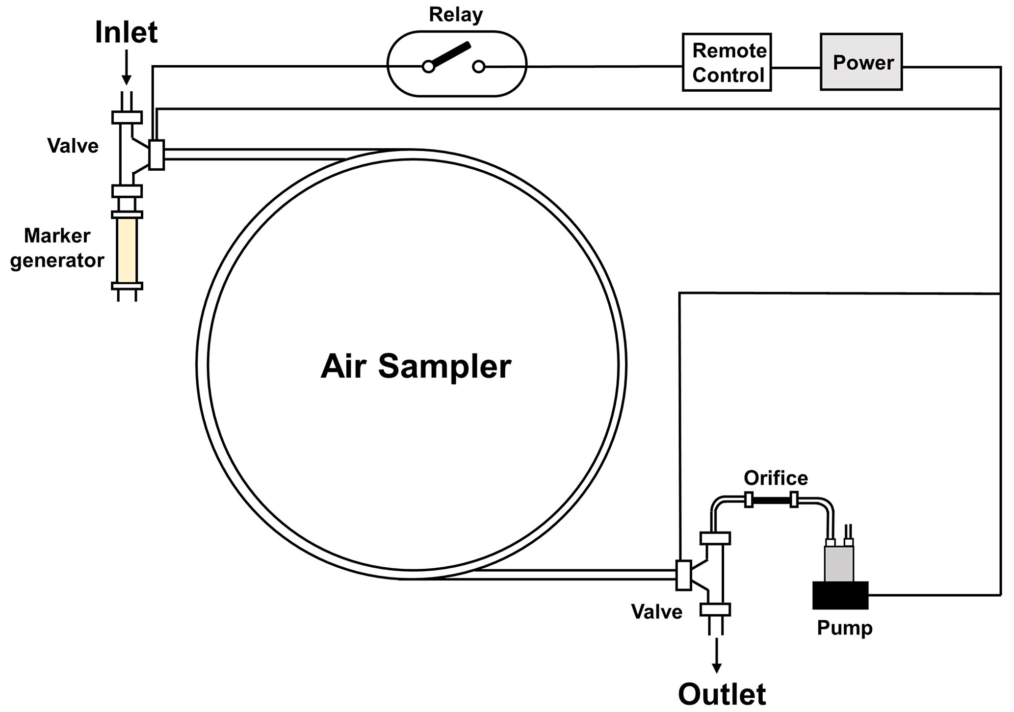
To realize GHG emission quantification by UAV measurement, a new compact air sampling system was developed based on a variation in the active AirCore method. The AirCore system contains a 150 m long stainless-steel tube, open at one end and closed at the other, that relies on positive changes in ambient pressure for passive sampling of the atmosphere (Karion et al., 2010). Figure 1 shows an overview of the patented design for this sampler. It consists of 150 m long thin-walled $\mathrm{1}/\mathrm{8}$ in. outside-diameter stainless-steel tubing, a pump, a micro-orifice, a CO₂ marker generator, two three-way solenoid valves and electric relays, with all electrical devices powered by a 12 V battery. The tubing is wound into a multilayer coil, in whose center the other components of the system are mounted. The system is housed in a highly compact patented carbon fiber assembly design of 280 mm diameter and 98 mm height that can be quickly mounted at and dismounted from the bottom of a UAV. The sampler weighs about 5.9 kg and allows for continuous sampling for up to 35 min.

Figure 1 Design of the air sampler.

The sampler air intake is mounted at 70 cm above the center of gravity of the UAV, placed near a sonic anemometer (below) for ensuring sampling of the same air mass as where wind speed is measured. The time stamp of the mixing-ratio observation was corrected for the short time lag of 4 s between sampling at the air intake and at the thin-walled stainless-steel tubing attributable to the length of the Teflon inlet tube. Shortly before every flight, the pump is remotely turned on to sample the CO₂ marker for 5 s and then to collect air samples. The CO₂ markers subsequently help in data extraction and analysis to identify the starting point and specific times during the UAV air sampling . During flight, the pump would alternatively sample the marker and the ambient air on a preset timing schedule. The sampling flow rate remains at 18 sccm during the entire flight, controlled with the micro-orifice which is placed between the pump and the coiled tubing. After landing, the pump is remotely turned off and the air sample in the sampling tubing is immediately analyzed with a cavity ring-down spectrometer (CRDS) (Picarro, Inc., CA, USA, model G2401) for CO₂ and CH₄ mixing ratios in the sampled air. Waiting longer would lead to unwanted mixing of the samples in the tubing. The air samples enter the tubing from the air inlet during sampling and leave the tubing from a different air outlet during later analysis. As a result, the samples at the beginning of the flight spend the same amount of time within the tubing as those at the end of the flight. Using the embedded CO₂ marker data, the CO₂ and CH₄ data series can be mapped to the sampling times and GPS locations during flight.

2.2 The 3-D sonic anemometer

Previous studies that applied UAV platforms for GHG monitoring generally relied on wind data from nearby ground weather stations (Morales et al., 2022; Allen et al., 2019). However, Gålfalk et al. (2021) show that wind speeds were inconsistent between a ground weather station at a 1.5 m height and an anemometer mounted on their UAV, especially when altitude increases, showing the need to have an onboard weather station for accurate flux calculations. In the present study, in order to obtain meteorological data along the flight track, a 3-D sonic anemometer (Geotech Inc, Denver, USA, model TriSonica Mini) is attached on the top of the UAV via a 450 mm carbon fiber pole. The anemometer measures three-component wind speed (U_x, U_y, w) and temperature (T). The measured data were further transformed into actual wind speeds and wind directions after corrections for UAV attitude (pitch, yaw, roll) changes and accounting for its airspeed, as well as the perturbations caused by the UAV rotor propellers using a patented correction algorithm. The GPS information, airspeed and attitude data (pitch, yaw, and roll) were extracted from the UAV data transmitted to the ground control station. The anemometer measures wind speeds within the range of 0 to 50 m s⁻¹, with an accuracy of ±0.1 m s⁻¹ below the wind speed of 10 m s⁻¹. The accuracy for wind direction measurement is ±1^∘. For temperature measurement, the operating range for the anemometer is between −40 and 85 ^∘C and the accuracy is ±2 ^∘C.

For anemometers mounted on multi-rotor UAVs, how to correct for the effects of the translational and rotational movements of the UAVs as well as the flows induced by the rotors to obtain accurate wind data is an ongoing research topic (Gålfalk et al., 2021; Wolf et al., 2017; De Boisblanc et al., 2014; Palomaki et al., 2017; Zhou et al., 2018). During flight, rotary wing UAVs create thrust by drawing air from above the rotors and expelling it downwards at a higher velocity. Such flows may extend to the anemometer position in addition to true atmospheric airflows, masking the true wind signals in the data from the anemometer (Wolf et al., 2017). Previous studies have conducted laboratory testing (Wolf et al., 2017; De Boisblanc et al., 2014; Palomaki et al., 2017) or flow field simulation (Zhou et al., 2018) to determine the appropriate distance to place anemometers onto multi-rotor UAVs to minimize the impact from the rotor-induced airflows. The anemometer in this research is mounted at an upward distance of 70 cm from the center of gravity of the UAV. A full digital model of the UAV, the anemometer and its mounting frame, and the air sampler was created. Using this digital model, computational fluid dynamics (CFD) simulations were performed to quantify wind speed disturbances caused by the UAV's rotor propellers to the anemometer during flight under a vast array of different wind conditions. An overall correction algorithm was developed in which parameters for propeller disturbances determined based on the CFD simulations were included along with correction schemes for false signals resulting from translational motions and changes in UAV pitch, roll and yaw.

2.3 The UAV

The air sampler and the anemometer are mounted on a hexacopter UAV (KWT-X6L-15). The UAV has a maximum flight time of ∼ 30 min at a maximum payload of 15 kg or longer with a lighter payload. Such flight endurance and carrying capacity meet our needs for loading the air sampler and the anemometer onto the UAV to realize emission quantification. The UAV is capable of flying in wind speeds of up to 14.4 m s⁻¹ to an altitude of about 4000 m and has a maximum horizontal flying speed of 18 m s⁻¹, a maximum ascending speed of 4 m s⁻¹ and a maximum descending speed of 3 m s⁻¹. The horizontal hovering precision of the GPS on the UAV is ±2 m, and the vertical hovering precision is ±1.5 m.

2.4 Air sample analysis

After landing, the air sample collected in the tubing is immediately analyzed with the CRDS analyzer. The withdrawal flow rate of the air from the sample tubing during analysis is an important parameter in optimizing the results. High withdrawal rates lead to unwanted mixing in the cavity of the analyzer. However, direct withdrawal of air from the sample tubing by the analyzer at a flow rate as low as the sampling flow rate of 18 sccm results in smoothing of concentrations from the inner-wall surface drag and desorption inside the tubing. We optimized the flow rate of the air from the sample tubing into the CRDS analyzer at ∼ 54 sccm, 3 times the sampling flow rate, by diluting the air sample with zero air, with two mass flow controllers separately controlling the flow rate of zero air and the withdrawal rate of the air sample (Fig. 2b).

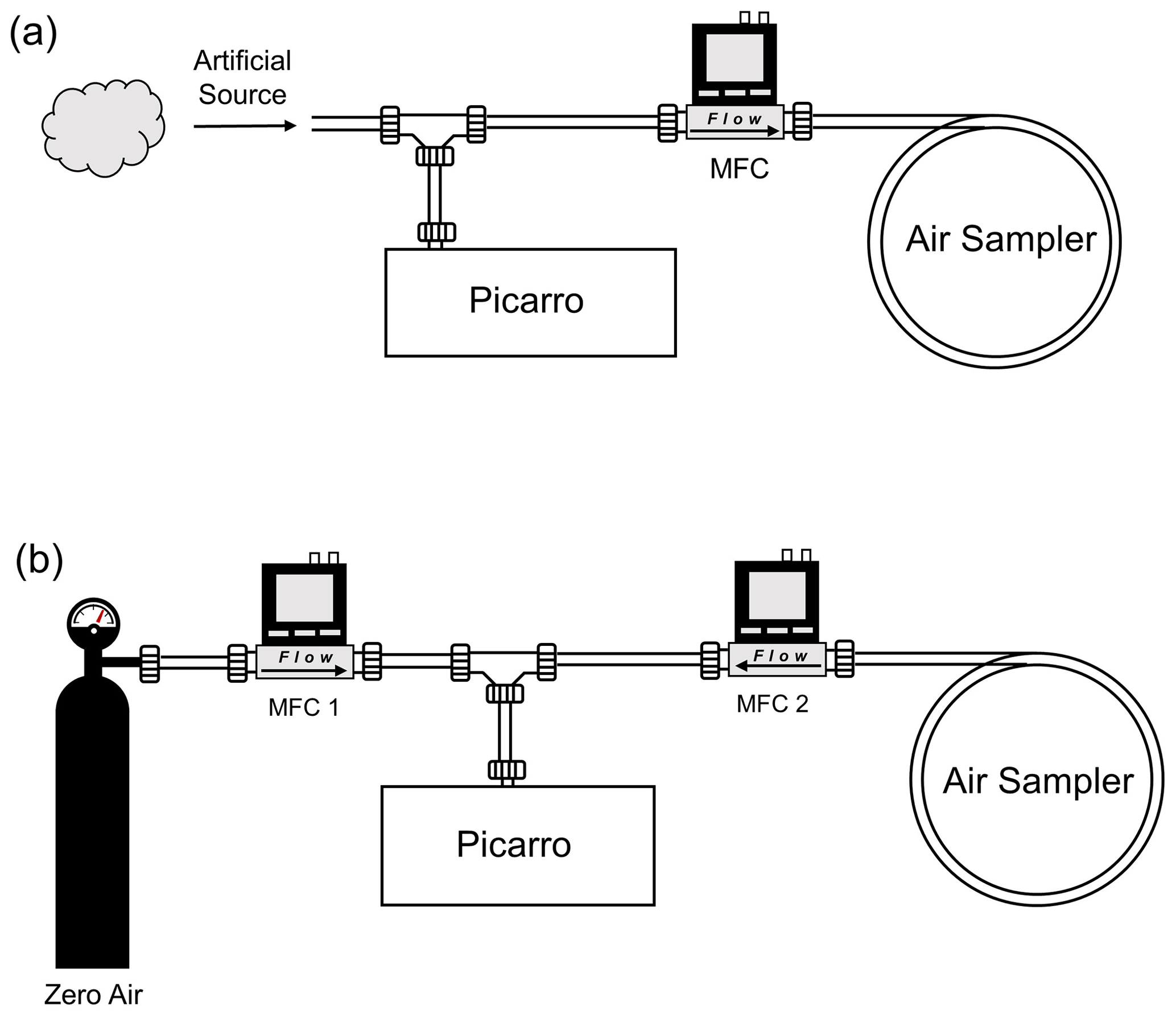
Figure 2 Diagram of the air sampler testing setup in the laboratory. (a) Simultaneous sampling by the air sampler and the Picarro CRDS analyzer. (b) Subsequent air sample analysis using the Picarro CRDS analyzer.

2.5 Mass-balance approaches for determining emission rates

The UAV-based measurements were coupled with the mass-balance approach TERRA to determine the emission rates of the measured pollutants using their measured mixing ratios and the meteorological data (three-component wind speed (U_x, U_y, w) and temperature (T)) collected on board the UAV during the flight. TERRA computes integrated mass fluxes through airborne virtual-box/screen measurements, including those made from aircraft and in this case UAVs. TERRA has been used successfully and extensively for emission rate determination of tens of volatile organic compounds (Li et al., 2017), CO₂ (Liggio et al., 2019), CH₄ (Baray et al., 2018), oxidized sulfur and nitrogen (Hayden et al., 2021), black carbon (Cheng et al., 2020), and secondary organic aerosol (Liggio et al., 2016) using aircraft measurements. To run TERRA based on a virtual-box flight, the first step is to map the CH₄ and CO₂ mixing-ratio data measured along the level flight tracks encircling a facility to the 2-D virtual walls of the virtual box, created from stacking the level flight tracks, that surrounds the facility. The 2-D virtual walls (or screens) are derived from the unwrapping of the virtual box to assist the presentation of the CH₄ and CO₂ plumes along the flight tracks, with the horizontal path length (i.e., the ground line projection of the fitted flight track) and altitude as the two dimensions. The start of the horizontal path is typically defined as the southeast corner of the virtual box, but the selection of this starting position has no effect on the emission rate computation, and the horizontal path distance increases in a counter-clockwise direction. This procedure results in a translation of each flight position point from a 3-D position of latitude (y), longitude (x) and altitude (z, meters above mean sea level) to a 2-D screen position of horizontal path distance $s=f(x,y)$. Subsequently, TERRA applies a simple kriging algorithm to interpolate the data and finally produces a mesh on the 2-D virtual box walls whose resolution can be set depending on applications. The kriging weights were obtained with an isotropic spherical semivariogram model. In TERRA, the nugget, sill and range can all be modified to fit the semivariogram model. The mixing ratios of both CH₄ and CO₂ are extrapolated from the lowest flight altitudes to the ground digital elevation using one of several methods or a combination thereof, namely (1) assuming a constant, (2) linear extrapolation between a constant and background, (3) a background value below flight altitudes, (4) a linear fit between the lowest flight altitude and zero at the ground, and (5) an exponential fit from the lower flight altitudes (Gordon et al., 2015). Concurrently measured wind speed from the UAV is decomposed into northerly and easterly components (U_N(s,z), U_E(s,z)) based on the wind direction and is similarly interpolated onto the 1 m × 2 m mesh. The decomposed wind speeds are further extrapolated to the ground digital elevation using a log profile fit (Gordon et al., 2015). Based on the interpolated/extrapolated CH₄ and CO₂ mixing ratio, temperature, pressure (calculated using the barometric height formula), and wind speeds, TERRA computes the fluxes of CH₄ and CO₂ through the virtual walls and finally their facility emission rates by integrating the fluxes.

To summarize, in TERRA the mass balance in computing the emissions within a control box for a given inert pollutant such as CH₄ or CO₂ is presented by

$$\begin{array}{}\text{(1)}& E_C=E_{C,\mathrm{H}}+E_{C,\mathrm{V}}-E_{C,\mathrm{M}},\end{array}$$

where E_C is the emission rate, E_C,H is the horizontal advective transfer rate through the box walls, E_C,V is the advective transfer rate through the box top and E_C,M is the increase in mass within the volume due to a change in air density. Other terms listed in the Gordon et al. (2015) computation algorithm that were used to solve for the total emission rate were often neglected as they contribute little to the total emission rates. Each term from Eq. (1) is estimated as

$$\begin{array}{}\text{(2)}& {\displaystyle }{E}_{C,\mathrm{H}}=M_{\mathrm{R}}\int \int X_C{\mathit{\rho }}_{\mathrm{air}}{U}_{\perp }\mathrm{d}s\mathrm{d}z,\text{(3)}& {\displaystyle }{E}_{C,\mathrm{V}}=M_{\mathrm{R}}{X}_{C,\mathrm{Top}}\int \int {\mathit{\rho }}_{\mathrm{air}}w\mathrm{d}x\mathrm{d}z,\text{(4)}& {\displaystyle }{E}_{C,\mathrm{M}}=M_{\mathrm{R}}\int \int \int X_C{\displaystyle \frac{\mathrm{d}{\mathit{\rho }}_{\mathrm{air}}}{\mathrm{d}t}}\mathrm{d}x\mathrm{d}y\mathrm{d}z,\end{array}$$

where M_R is the ratio of the compound molar mass to the molar mass of air, X_C(s,z) is the mixing ratio of the compound in question, ρ_air(s,z) is the air density, w is the vertical wind velocity at the box top, X_C,Top is the mixing ratio at the top of the box, and $U_{\perp }(s,z)$ is the horizontal wind vector normal to the flight track calculated from the northerly and easterly components (U_E(s,z), U_N(s,z)):

$$\begin{array}{}\text{(5)}& U_{\perp }(s,z)={\displaystyle \frac{U_{\mathrm{N}}(s,z)\mathrm{d}s/\mathrm{d}x-U_{\mathrm{E}}(s,z)\mathrm{d}s/\mathrm{d}y}{\sqrt{{\left(\mathrm{d}s/\mathrm{d}x\right)}^{\mathrm{2}}+{\left(\mathrm{d}s/\mathrm{d}y\right)}^{\mathrm{2}}}}}.\end{array}$$

The vertical transfer rate term E_C,V is estimated by computing the air mass vertical transfer rate, determined from air mass balance within the box, and multiplying it with the CO₂ or CH₄ mixing ratios at the box top. This term is normally negligible in other top-down emission estimate approaches since it is typically minuscule compared to horizontal fluxes, but it can affect the computed emission rates when vertical air movement becomes more significant, such as under unstable atmospheric conditions. E_C,M is often ignored in other mass-balance approaches; in TERRA it is estimated by taking the time derivative of the ideal gas law in temperature and pressure during the flight time, and typically it does not change significantly over the duration of 30 min or so for the UAV flight.

To suit the UAV measurements, the following modifications to the TERRA algorithm were made: (1) a much higher interpolation resolution for the kriging mesh was implemented for application to the UAV measurements in this study, with the interpolation mesh size adjusted to 1 m (vertical) by 2 m (horizontal), as UAVs fly significantly shorter distances compared to applications to piloted aircraft for which the interpolation resolution was 20 m (vertical) by 40 m (horizontal); (2) the modified TERRA now applies an embedded routine to automatically fit flight tracks using least squares, while this procedure was previously conducted manually offline through an geographic information system when using TERRA; and (3) the modified version of TERRA has added an algorithm for correcting negative weights during kriging interpolation following Deutsch (1995). TERRA was updated at Peking University, was recoded using the Python language, and runs under a browser–server environment with a new graphical user interface (GUI) and new interactive data flow.

3 Laboratory tests

3.1 Validation of the air sampler

Prior to flights in the field, we validated the air sampler in laboratory experiments by first sampling artificial air while making simultaneous online measurements of the artificial air with the CRDS analyzer, then analyzing the sampled artificial air with the same CRDS analyzer and finally comparing the results from the air sampler to the online measurements. An experimental apparatus was constructed for the simultaneous sampling of the same artificial air with the air sampler and the CRDS analyzer through a tee junction (Fig. 2a) and for subsequent air sample analysis using the same CRDS analyzer (Fig. 2b). In the artificial air, CH₄ and CO₂ standards were control-released into the lab air from an 8 L gas cylinder filled with a gas mixture of 5 ppm CH₄, 2 ppm CO and 600 ppm CO₂ to generate the artificial air source. The outlet of the standard gas cylinder was held at varying distances to the tee junction over time to yield a time series of different CH₄ and CO₂ mixing ratios, which were designed to mimic plumes expected in the real atmosphere. During analysis, the flow rate through the zero air (Mass Flow Controller 1) is adjusted to make sure that the flow rate through the air sampler (Mass Flow Controller 2) is stable and consistent at 54 sccm (Sect. 2.4).

Figure 4a illustrates the mixing ratios of CO₂ and CH₄ time series obtained from the air sampler and online measurements by the CRDS analyzer. It can be seen that the measured results from the air sampler and the online CRDS analyzer measurements are in good agreement throughout the tests, and the correlation coefficient is estimated to be 0.89 and 0.73 for CH₄ and CO₂ (Fig. 4c and f). For the measurements with the air sampler, short-term variations and noise in the CH₄ and CO₂ mixing ratios, which were fully captured by the CRDS analyzer during the online measurements, were smoothed out, while the main features and tendencies were preserved. In fact, the air sampler measurement results should be a smoothed version of the CRDS analyzer online measurements due to mixing in the analyzer cavity, molecular diffusion during sample storage in the sampler, inner-wall surface drag and desorption during the sample's withdrawal from the tubing during analysis, as well as Taylor dispersion during sampling and analysis (Karion et al., 2010). Dilution with zero air during later CRDS analysis also contributes to the smoothing.

3.2 Data deconvolution to achieve high time resolution

While it is impractical to delineate the individual smoothing effects when the air sample passes through the coupled system of the sampler plus the analysis setup as described above, the measured concentration y(t) can be treated as a result of the convolution of the air concentration before sampling x(t) and of a smoothing kernel g(i) consisting of a series of weights, which are inherently determined by factors including the sampler properties (tubing length, inner diameter, temperature, absorptive properties, flow rates), storage time, dilution and mixing in the cavity of the instrument. The smoothing can be described as

$$\begin{array}{}\text{(6)}& \begin{array}{rl}y\left(t\right)& ={\sum }_{i=r}^{s}g\left(i\right)x(t-i)+n\left(t\right),\\ & t=s,s+\mathrm{1},\mathrm{\dots },n-\mathrm{1}+r\end{array}\end{array}$$

or expressed as a convolution of the form

$$\begin{array}{}\text{(7a)}& y\left(t\right)=g\left(t\right)\times x\left(t\right)+n\left(t\right),\end{array}$$

where y(t) is the measured concentration at time t; x(t) the air concentration; and n(t) the unknown noise, assumed to be independent of x(t). The kernel g(i) contains $s-r+\mathrm{1}$ non-zero kernel weight terms ($\mathrm{0}<g\left(i\right)<\mathrm{1}$). When all four terms in Eq. (7a) undergo Fourier transform, Eq. (7a) can be expressed in the frequency domain as follows:

$$\begin{array}{}\text{(7b)}& Y\left(f\right)=G\left(f\right)X\left(f\right)+N\left(f\right).\end{array}$$

In order to characterize the kernel weights g(i), a second lab experiment was conducted during which the sampler first sampled zero air for some time and then sampled the CO₂ and CH₄ standards for 1 s, before returning to sampling zero air again, creating an original concentration pulse signal in the x(t):

$$\begin{array}{}\text{(8)}& x\left(t\right)=\left\{\begin{array}{cc}C,& t=j\\ \mathrm{0},& t\ne j\end{array}\right.,\end{array}$$

where j is the jth second when the sampler collected the standard of a known concentration C. This air sample was then analyzed with the CRDS as described above. After sampling, storing and analyzing, smoothing of the original concentration pulse leads to the concentration signal output Y(t) as follows:

$$\begin{array}{}\text{(9)}& \begin{array}{rl}& y\left(t\right)\\ & =\left\{\begin{array}{cc}{\sum }_{i=r}^{s}g\left(i\right)x(t-i)+n\left(t\right)& t-i=j\text{and}i=r,\\ =g(t-j)C+n\left(t\right),& r+\mathrm{1},\mathrm{\dots },s\\ n\left(t\right),& t-i\ne j\end{array}\right.,\end{array}\end{array}$$

where y(t) is the measured concentrations from the air sampler after sampling the concentration pulse and is non-zero when $t-i=j$, with the index i taking the values from r to s. The noise n(t) term is zero for $t-i\ne j$ and can be assumed to have similar behavior for $t-i=j$. Therefore,

$$\begin{array}{}\text{(10)}& \begin{array}{rl}g\left(i\right)& =g(t-j)={\displaystyle \frac{\mathrm{1}}{C}}y\left(t\right)-{\displaystyle \frac{\mathrm{1}}{C}}n\left(t\right),t=i+j\\ & \text{and}i=r,r+\mathrm{1},\mathrm{\dots },s.\end{array}\end{array}$$

The second lab experiment showed that y(t), and therefore the kernel g(t), consists of 70 non-zero values. To remove the noise n(t), g(t) is further smoothed using a box-car running mean of five terms:

$$\begin{array}{}\text{(11)}& \begin{array}{rl}\widehat{g}\left(t\right)& ={\displaystyle \frac{\mathrm{1}}{\mathrm{5}}}{\sum }_{k=t-\mathrm{2}}^{k=t+\mathrm{2}}g\left(k\right)\approx {\displaystyle \frac{\mathrm{1}}{C}}y\left(t\right),t=i+j\\ & \text{and}i=r,r+\mathrm{1},\mathrm{\dots },s.\end{array}\end{array}$$

It could be seen from Fig. 3 that $\widehat{g}\left(t\right)$ has an asymmetrical distribution with a right-trailing tail and a half-height width of approximately 20 s for CO₂ and 21 s for CH₄, indicating that the smoothing had significantly reduced the sampling/analysis method time resolution to about 20 s from the 1 s resolution of the original pulse in the air concentration. The kernel shows that the influence that the neighboring points have on a given point decreases with increases in the gap between the two points.

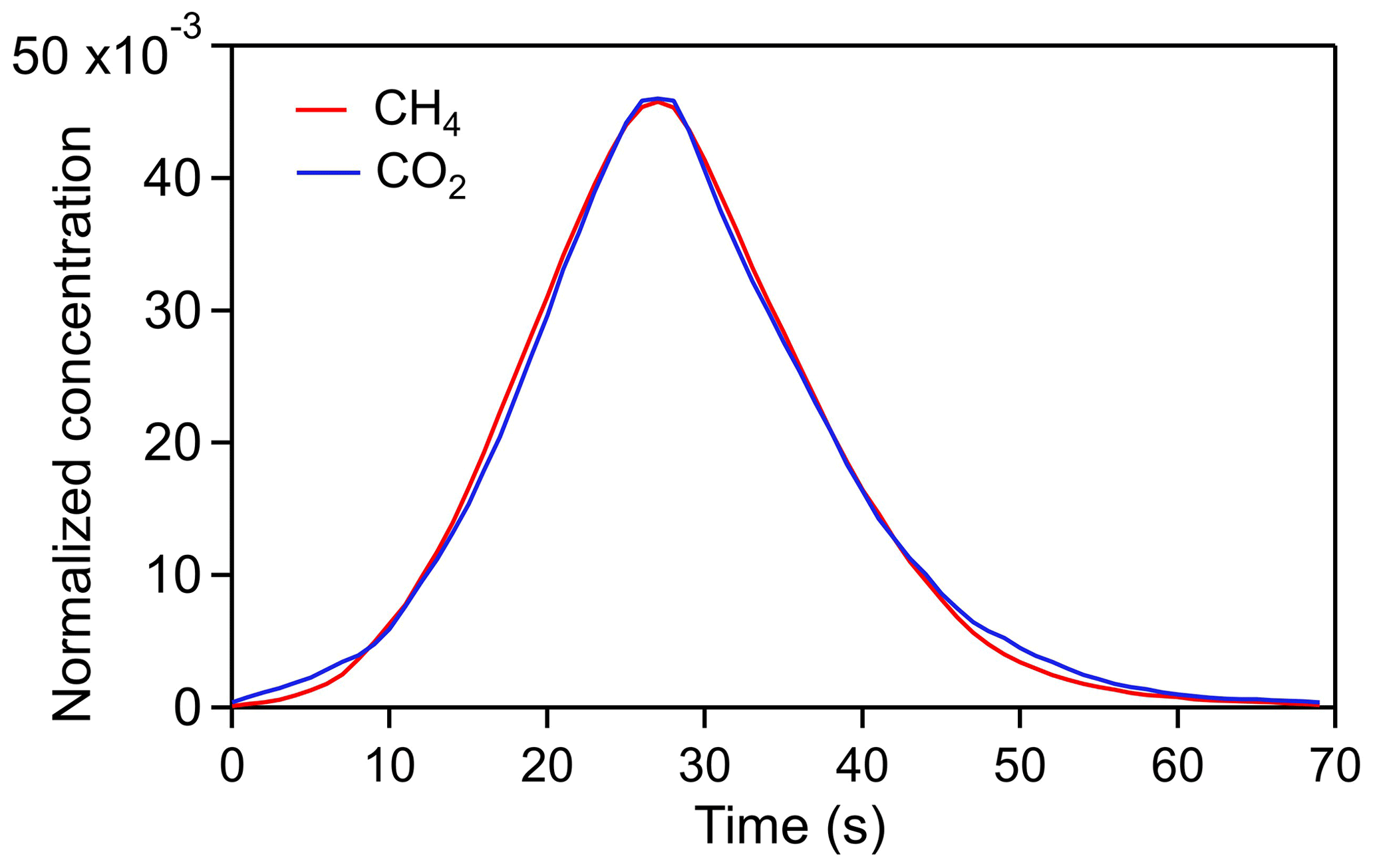
Figure 3 The output of the 1 s signal after sampling, storing and analyzing using the air sampler for CO₂ and CH₄, normalized by their respective concentrations in the standard. As shown in the text, these curves are the actual kernel weights of $\widehat{g}\left(t\right)$.

To test whether the kernel weights $\widehat{g}\left(t\right)$ can smooth the online measured concentrations from the first lab experiment (top line in Fig. 4a and b), the weights $\widehat{g}\left(t\right)$ were used to convolute with the data from the online measurements (i.e., x(t)), resulting in an estimated $\widehat{y}\left(t\right)$ (Fig. 4a and b, third line) that is in excellent agreement with the measurements from the air sampler, with the correlation coefficients increased to 0.99 and 0.98 for CH₄ and CO₂ (Fig. 4d and g).

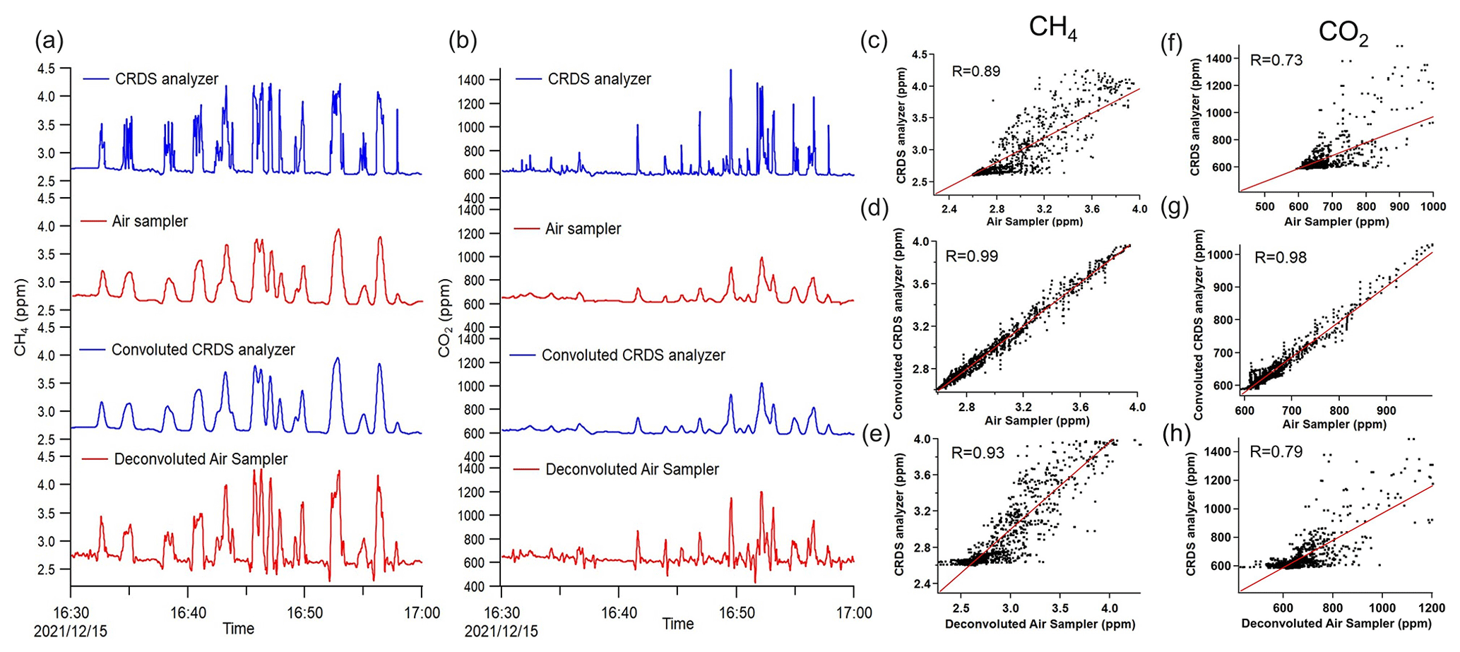
Figure 4 (a, b) Mixing ratios of CO₂ and CH₄ measurements by online measurements with CRDS (the first line) and the air sampler (the second line) in laboratory tests. The third line represents the smoothed CRDS data after convolution with the kernel $\widehat{g}\left(t\right)$, and the fourth line represents the deconvoluted series after Wiener deconvolution. The signals of the same color represent the original signals and the corresponding signals after convolution or deconvolution. The date format is year/month/day, and the time is local time. (c–e) Correlation plots of CH₄. (f–h) Correlation plots of CO₂.

The ultimate goal of determining $\widehat{g}\left(t\right)$ in Fig. 3 is to deconvolve y(t) from the air sampler to obtain the original concentration series x(t) using a number of deconvolution techniques. In the present study, we used the deconvolution method based on the Wiener theorem (Lin and Jin, 2013). The theorem provides the Wiener convolution filter h(t) so that x(t) can be estimated as follows:

$$\begin{array}{}\text{(12)}& \widehat{x}\left(t\right)={\sum }_{i=-\mathrm{\infty }}^{\mathrm{\infty }}h\left(i\right)y(t-i)=h\left(t\right)\times y\left(t\right),\end{array}$$

where y(t) is the measured concentration, and $\widehat{x}\left(t\right)$ an estimate of x(t). In the frequency domain, Eq. (12) may be rewritten as a product of two scalars:

$$\begin{array}{}\text{(13)}& \widehat{X}\left(f\right)=H\left(f\right)Y\left(f\right),\end{array}$$

where $\widehat{X}\left(f\right)$, H(f) and Y(f) are the Fourier transforms of $\widehat{x}\left(t\right)$, h(t) and y(t), respectively. The Wiener convolution filter h(t) is derived from the minimization of the mean square error:

$$\begin{array}{}\text{(14)}& \mathit{ϵ}\left(f\right)=E{\left|X\left(f\right)-\widehat{X}\left(f\right)\right|}^{\mathrm{2}},\end{array}$$

with E denoting the expectation. When Eqs. (7b) and (13) are substituted into Eq. (14) and the quadratic is expanded, the mean square error ϵ(f) can be differentiated with respect to H(f) and the derivative $\frac{\mathrm{d}\mathit{ϵ}\left(f\right)}{\mathrm{d}H\left(f\right)}$ is set to zero to achieve the minimization; under the assumption that the noise N(f) is independent of X(f), H(f) is derived as

$$\begin{array}{}\text{(15)}& H\left(f\right)={\displaystyle \frac{G\left(f\right)S\left(f\right)}{{\left|G\left(f\right)\right|}^{\mathrm{2}}S\left(f\right)+N\left(f\right)}},\end{array}$$

where G(f) is the Fourier transform of $\widehat{g}\left(t\right)$ derived from the second lab experiment described above S(f)=E|X(f)|² and N(f)=E|N(f)|² are the mean power spectral densities of the original concentration series x(t) and the noise n(t), respectively. Equation (15) could be rewritten as

$$\begin{array}{}\text{(16)}& \begin{array}{rl}H\left(f\right)& ={\displaystyle \frac{\mathrm{1}}{G\left(f\right)}}\left[{\displaystyle \frac{{\left|G\left(f\right)\right|}^{\mathrm{2}}}{{\left|G\left(f\right)\right|}^{\mathrm{2}}+N\left(f\right)/S\left(f\right)}}\right]\\ & ={\displaystyle \frac{\mathrm{1}}{G\left(f\right)}}\left[{\displaystyle \frac{{\left|G\left(f\right)\right|}^{\mathrm{2}}}{{\left|G\left(f\right)\right|}^{\mathrm{2}}+\mathrm{1}/\text{SNR}\left(f\right)}}\right],\end{array}\end{array}$$

where $\text{SNR}\left(f\right)=S\left(f\right)/N\left(f\right)$ is the signal-to-noise ratio.

Substituting Eq. (16) into Eq. (13), $\widehat{X}\left(f\right)$, the Fourier transform of $\widehat{x}\left(t\right)$, is derived. The deconvolution is completed with the inverse Fourier transform of $\widehat{X}\left(f\right)$ to give $\widehat{x}\left(t\right)$, the estimated air concentrations. The deconvolved series of CH₄ and CO₂ restored with the Wiener convolution filter are shown in Fig. 4a and b, and the correlation coefficients between the deconvoluted results and the online measurements with the CRDS analyzer are 0.93 and 0.79 for CH₄ and CO₂ (Fig. 4e and h), higher than those between the original air sampler measurement and the CRDS analyzer. These results indicate the effectiveness of the Wiener theorem in deconvolving a smoothed series to a much higher time resolution while accounting for noise. The restored series is improved in terms of time resolution, from about 20 s mentioned above to about 3–4 s after the deconvolution. The lab test data from the online measurements contain strong high-frequency components, artificially manipulated to provide an extreme case for testing the deconvolution algorithm. Such high frequencies lead to some residual noise in the deconvolved results, primarily as a result of choosing the cutoff frequencies for the mean power spectral densities S(f) and N(f). Nevertheless, such a situation will be improved for sampling in the real atmosphere where sub-second high-frequency variations are not common.

4 Field application

To apply the UAV-based measurement system described above to atmospheric measurements of CO₂ and CH₄, flights were made at the Shagang Group located in Jiangsu, China, on 28 December 2021. The Shagang Group is a major iron and steel company on the south shore of the Yangtze River (31.9704^∘ N, 120.6443^∘ E). The company produces over 40×10⁶ t of steel each year, making it one of China's top five steel producers. On-site coke making for iron production is located in the western part of the Shagang steel complex. The coke-making process is to dry distill coal in a coking oven at ∼ 1000 ^∘C temperature to boil off volatile components to form coke (metallic coal). During coke production, combustion of coking oven gas, blast furnace gas from steel making and coal tar plus light oil for heating the coking oven are the main CO₂ and CH₄ emission sources.

Two coking plant stacks were chosen as the target emission source for the field UAV flight. During flight, the UAV was flown in a rectangular pattern (200 m × 500 m) that encloses the two stacks, with repeated flight tracks at nine altitude levels that, when stacked, created a virtual box and intercepted the emitted CO₂ and CH₄ plumes on the downwind side of the box. The UAV ascended from the ground to 135 m a.g.l. and started the box flight at this altitude, ascending 15 m every level and reaching a maximum altitude of 255 m a.g.l. before landing. The UAV maintained a constant horizontal speed of 8 m s⁻¹ during flight. The flight lasted for approximately 30 min. It is assumed that the plume remains steady during the time of measurement. After landing, the air sample collected in the sampler was immediately analyzed with the CRDS analyzer as per the procedure depicted above in Fig. 2b.

5 Result and discussion

5.1 CH₄ and CO₂ mixing-ratio enhancement from the coking plant

Figure 5a shows the time series of CH₄ and CO₂ mixing ratios measured with the air sampler at the coking plant during the flight (red line). The air sampler sampled for a total of 30 min during the flight. After landing, the air sample was analyzed for 10 min, as the analysis flow rate triples the sampling flow rate (54.0 sccm vs. 18.0 sccm). The timescales of instrument readings were then stretched three times to restore the original timescales. The CH₄ and CO₂ time series were then deconvolved using the convolution kernel obtained from laboratory test (Sect. 3.2) to restore the mixing-ratio time series in air (black line). The meteorological parameters during the time of flight were measured by the 3-D anemometer, showing consistent southwesterly winds (Fig. 5b). The average wind speed is 4.7±4.9 m s⁻¹, and the average wind direction is 216.4±38.4^∘ during the time of flight. Consistency of wind measurements can be seen from the two wind rose plots for the northern wall and the southern wall, respectively. During the flight, the maximum mixing ratio measured was 5.6 ppm for CH₄ and 1356 ppm for CO₂. During the 30 min flight, a total of five CO₂ makers were generated during the 30 min of sampling (Fig. 5a), and the decreases in the marker concentrations are corrected with a Gaussian form function.

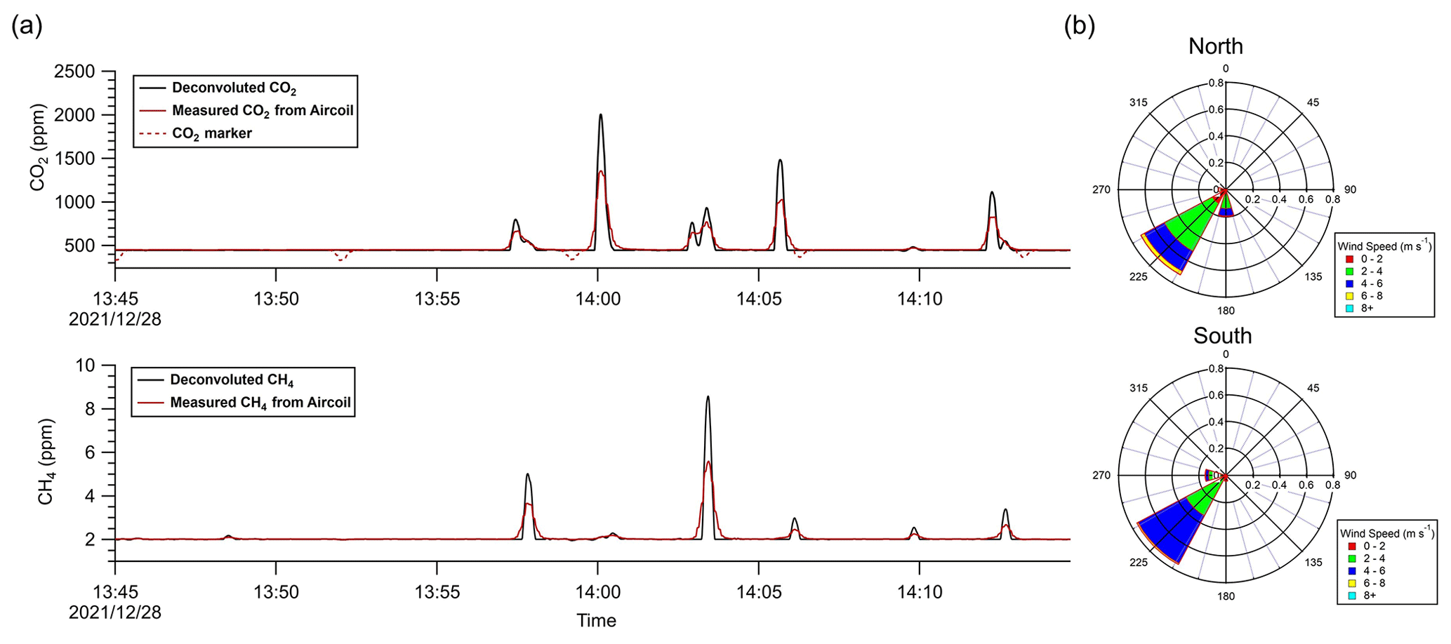
Figure 5 (a) The red line represents CH₄ and CO₂ mixing ratios measured from the air samples collected with the air sampler during the flight at the coking plant. The black line represents the deconvolved CH₄ and CO₂ time series, and the dashed-red-line sections represent the original marker CO₂ concentrations every 7 min. (b) Wind rose plots for the northern and southern wall based on the onboard meteorological measurements during the flight.

5.2 Emission estimation

The CO₂ and CH₄ emission rates for the stacks from the coking plant were estimated by applying a version of the computation algorithm TERRA specifically modified to suit UAV measurements. The deconvolved mixing-ratio time series of CO₂ and CH₄ were used in the TERRA algorithm. The algorithm first maps the mixing ratios to the walls of the virtual box, then applies a kriging scheme to interpolate the data and produces a 2 m (vertical) by 1 m (horizontal) mesh on the virtual box walls (200 m × 500 m) (Fig. 6). The semivariogram of the flight points was fitted with a spherical model (range = 300, sill = 3, nugget = 0). Wind speed and wind direction are first decomposed into northerly and easterly components and then further converted to vectors that are normal to and parallel to the walls of the virtual box before kriging. Background CH₄ and CO₂ were determined using upwind measurements. The background between upwind data was linearly interpolated and box-car-smoothed within a 3–4 min moving window to derive a variable baseline CH₄ and CO₂ for the entire 30 min flight. As shown in Fig. 6, the CH₄ and CO₂ plumes can be seen at different locations on the downwind side of the box wall, which indicates that the CH₄ plume and the CO₂ plume probably came from different sources within the box. Using the modified version of TERRA, the emission rates for the two stacks in the coking plant were calculated to be 0.12±0.01 t h⁻¹ for CH₄ and 110±20 t h⁻¹ for CO₂. The uncertainties for the estimates were derived from detailed analyses of each uncertainty source including measurement error in the mixing ratio and wind speed, the near-surface wind extrapolation, the near-surface mixing-ratio extrapolation, the box-top mixing ratio, the box-top height, and deconvolution.

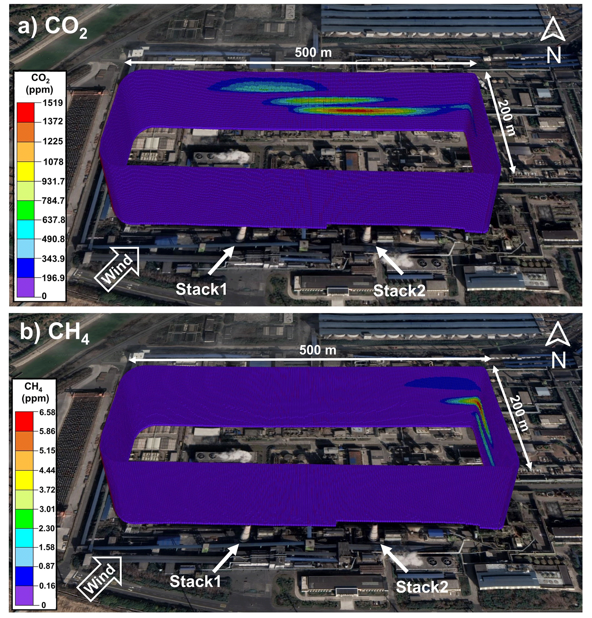
Figure 6 Virtual flight box for monitoring CO₂ (a) and CH₄ (b) during the flight. The CO₂ and CH₄ plumes were captured on the north and east wall, respectively. The wind came from the southwestern direction. Satellite imagery ©Google Earth 2019.

5.3 Uncertainty analysis

To determine the overall uncertainty in the emission rates, each source of uncertainty contributing to the overall uncertainty needs to be identified and quantified. For the emission rate quantification from UAV measurement, the sources of uncertainties include the following: measurement uncertainties in the mixing ratios and wind speeds (δ_M), the near-surface wind extrapolation (δ_Wind), the near-surface mixing-ratio extrapolation (δ_Ex), the box-top mixing ratio (δ_Top), box-top height (δ_BH), and uncertainties due to data deconvolution as shown in the main text (δ_Deconv). Each uncertainty is treated as an independent estimate, and all uncertainties are propagated in quadrature to determine the overall uncertainty in the estimated emission rate:

$$\begin{array}{}\text{(17)}& {\mathit{\delta }}^{\mathrm{2}}={\mathit{\delta }}_{\mathrm{M}}^{\mathrm{2}}+{\mathit{\delta }}_{\mathrm{Wind}}^{\mathrm{2}}+{\mathit{\delta }}_{\mathrm{Ex}}^{\mathrm{2}}+{\mathit{\delta }}_{\mathrm{Top}}^{\mathrm{2}}+{\mathit{\delta }}_{\mathrm{BH}}^{\mathrm{2}}+{\mathit{\delta }}_{\mathrm{Deconv}}^{\mathrm{2}}.\end{array}$$

The accuracy of the mixing-ratio measurements from the Picarro CRDS analyzer is 50 and 1 ppb for CO₂ and CH₄, respectively. By adding variations in the measured mixing ratios based on the measurement accuracies and re-applying TERRA, the derived emission rates varied within 1 % for both CO₂ and CH₄. Thus, the uncertainties in the emission rates due to mixing-ratio measurements (δ_M) were estimated at 1 % for both CH₄ and CO₂.

The anemometer measures wind speeds with an accuracy of ±0.1 m s⁻¹ at wind speeds < 10 m s⁻¹ and wind directions with an accuracy of ±1^∘. The uncertainty in the wind measurements (δ_Wind) was estimated using error propagation in the normal wind $U_{\perp }(s,z)$, as it is calculated from the northerly and easterly wind components and thus from wind speed (WS) and wind direction (WD):

$$\begin{array}{}\text{(18)}& {\displaystyle }{\mathit{\delta }}_{U_{\perp }}=\sqrt{{\mathit{\delta }}_{\mathrm{easterly}}^{\mathrm{2}}+{\mathit{\delta }}_{\mathrm{northerly}}^{\mathrm{2}}+\mathrm{2}{\mathit{\sigma }}_{\mathrm{easterly}-\mathrm{northerly}}},\text{(19)}& {\displaystyle }{\mathit{\delta }}_{\mathrm{easterly}}=\left|\text{WScos}\left(\text{WD}\right){\mathit{\sigma }}_{\mathrm{WD}}\right|,\text{(20)}& {\displaystyle }{\mathit{\delta }}_{\mathrm{northerly}}=\left|\text{WSsin}\left(\text{WD}\right){\mathit{\sigma }}_{\mathrm{WD}}\right|.\end{array}$$

Using this calculation, the uncertainty in the normal wind ${\mathit{\delta }}_{U_{\perp }}(s,z)$ was derived at each location. The uncertainty that contributed to the total emission rates was examined by setting the normal wind to its upper and lower bounds defined by its uncertainty range and followed by computing the emission rates using TERRA. The derived CH₄ and CO₂ emission rates varied by 1.5 % and 1.9 %, respectively. Hence the uncertainties from wind speed measurements (δ_Wind) were conservatively estimated to be 2 % for both CH₄ and CO₂.

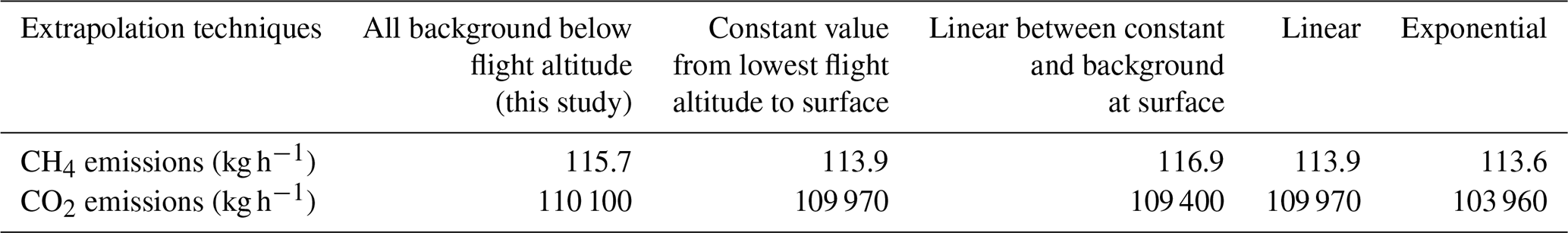
Due to a lack of near-surface measurements along the box walls, extrapolation of CH₄ and mixing ratios from the lowest flight path (∼ 150 m above ground level) to the ground level has been shown to be a source of potentially large uncertainty within TERRA. The magnitude of the uncertainty depends on the nature of the emissions; for example, surface emissions which may not be fully captured by the flight altitude range have higher uncertainties at ≈ 20 %, whereas elevated stack emissions which are fully captured by the flight altitude range lead to much smaller uncertainties of < 4 % in the emission estimates (Gordon et al., 2015). In the present study, to estimate uncertainties due to extrapolating mixing ratios from the lowest flight track to the ground (δ_Ex), results from all extrapolation techniques (i.e., linear to the ground, constant value to the ground, linear to background value, or some combination of methods) were derived and compared with the result using a background value below flight altitudes (Table 1). Therefore, this term of uncertainty was evaluated at 2 % and 6 % for CH₄ and CO₂, respectively.

Table 1 Emission rates derived using different extrapolation techniques.

Additional components contributing to uncertainties in the computed emission rates specific to the box approach include the box-top mixing ratio (δ_Top) and box-top height (δ_BH). The TERRA box approach assumes a constant mixing ratio at the box top (X_C,Top) by averaging the measured value at the top level. The term δ_Top is determined from the 95 % confidence interval ($\mathrm{2}\mathit{\sigma }/\surd n$) of the interpolated measurements. The calculated confidence interval of the mixing ratio at the box top is 0.01±0.13 ppm for CH₄ and 70.1±89.1 ppm for CO₂. Top average mixing ratios of 0.14 ppm for CH₄ and 159.2 ppm for CO₂ are set as input parameters to derive resulting uncertainties in the emissions rates. Thus, 106.6 kg h⁻¹ for CH₄ and 93 760 kg h⁻¹ for CO₂ were derived. Then, this uncertainty term is conservatively taken as 8 % and 16 % for CH₄ and CO₂.

The uncertainty due to the choice of box height, δ_BH, within TERRA is estimated by recomputing the emission rate with a reduced box height (z) of 100 m. The recalculated emission rate after reducing the box height of 100 m is 106.4 kg h⁻¹ for CH₄ and 113 500 kg h⁻¹ for CO₂; thus δ_BH is estimated as 8 % for CH₄ and 3 % for CO₂.

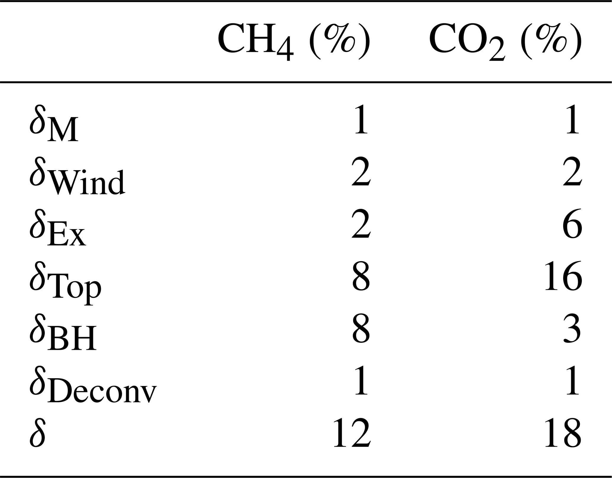
For cases that use the air sampling system instead of online measuring instruments, as the CH₄ and CO₂ time series measured from the air sampler were deconvoluted to restore the unsmoothed time series before being input into the TERRA algorithm, it is necessary to account for the uncertainty that comes from such deconvolution as outlined in the main text. Time series before and after deconvolution were applied to the TERRA algorithm to obtain the total emission rates. The computations show that emission rates before and after deconvolution vary within 1 %, which was taken as the uncertainty δ_Deconv. The assessment of uncertainties for the TERRA-computed emission rates from the coking plant is given in Table 2.

Table 2 Assessment of percent uncertainties for CH₄ and CO₂ emission rate estimations. The sources of uncertainties include the following: measurement uncertainties in the mixing ratios and wind speeds (δ_M), the near-surface wind extrapolation (δ_Wind), the near-surface mixing-ratio extrapolation (δ_Ex), the box-top mixing ratio (δ_Top), box-top height (δ_BH), and uncertainties due to data deconvolution as shown in the main text (δ_Deconv).

5.4 Comparison with Gaussian inversion approach

The TERRA computation results can be further evaluated. Of the multiple CH₄ plumes that were captured on the north and east walls of the virtual box, the largest CH₄ one resembles a nearly perfect Gaussian plume distribution and is clearly associated with the east stack of the two, for which the emission rate may be recalculated using the Gaussian plume model. The Gaussian plume model makes basic assumptions that the plume is emitted from a point source and that the atmospheric turbulence is constant in space and time (Visscher, 2014). In this study, the captured plume was completely elevated and thus not constrained by boundaries. In the absence of boundaries, the equation for pollutant mixing ratios in Gaussian plumes is as follows:

$$\begin{array}{}\text{(21)}& c={\displaystyle \frac{Q}{\mathrm{2}\mathit{\pi }\stackrel{\mathrm{‾}}{u}{\mathit{\sigma }}_y{\mathit{\sigma }}_z}}\exp \left(-{\displaystyle \frac{y^{\mathrm{2}}}{\mathrm{2}{\mathit{\sigma }}_y^{\mathrm{2}}}}\right)\exp \left(-{\displaystyle \frac{(z-h{)}^{\mathrm{2}}}{\mathrm{2}{\mathit{\sigma }}_z^{\mathrm{2}}}}\right),\end{array}$$

where c is the concentration at a given position x, y and z (g m⁻³); Q is the emission rate (g s⁻¹); $\stackrel{\mathrm{‾}}{u}$ is the mean wind speed (m s⁻¹); h is the effective source height (m); and σ_y and σ_z are dispersion parameters in the horizontal (lateral) and vertical directions, respectively (m).

The dispersion parameters σ_y and σ_z were obtained by fitting the spatial distribution of CH₄ mixing ratios on the measurement screen into a Gaussian function. As the wall intercepting the plume is not perpendicular to the wind direction, the plume was projected to a different virtual wall perpendicular to the wind direction before fitting the Gaussian function. By calculating the standard deviations of the Gaussian distributions in the y and z directions, σ_z is estimated to be 6.3±0.3 m and σ_y is 15.7±0.4 m. The downwind measurement plane is examined to find the point with the highest CH₄ mixing ratio of 6.575 ppm and its location (s=160 m, z=217 m). For the separate CH₄ plume, the Gaussian plume model gives an emission rate of 40±6.8 kg h⁻¹. The uncertainty is quantified by considering the accuracy of the mixing-ratio measurement, the variation in wind speed and the confidence interval for the dispersion parameters given by Gaussian function fitting. CH₄ measurement uncertainties from the instrument comprise < 1 %. The uncertainty contributed by the mean wind speed estimation was examined by varying the average wind speed by the standard deviation of the wind data around the plume (3.8±0.6 m s⁻¹), followed by input into Gaussian plume model. This mean wind speed sensitivity analysis resulted in CH₄ emission rates that varied by 16 %. The same sensitivity analysis was done with σ_y (15.7±0.4 m) and σ_z (6.3±0.3 m), which resulted in CH₄ emission rates that varied by 4 % and 3 %, respectively. Thus, the total uncertainty is added in quadrature to be 17 %. The TERRA algorithm is able to obtain the emission rate for a selected section through a certain area of the screen. For this isolated CH₄ plume, the TERRA algorithm computed an emission rate of 65±8 kg h⁻¹, which is comparable to the emission rate estimation from the Gaussian plume model.

5.5 Validation of UAV-based emissions and comparison with IPCC-based emissions

The coking process is one of the most energy-consuming operations during iron and steel production and tends to emit large amounts of CO₂ and CH₄. According to the Chinese national GHG inventory report, CO₂ and CH₄ emissions from coke production in iron and steel production processes were calculated using the Tier-1 method in the IPCC Guidelines (Ministry of Ecology and Environment of China, 2018). In the Tier-1 method, default emission factors for coke production are used to estimate the CO₂ and CH₄ emissions without considering local variations:

$$\begin{array}{}\text{(22)}& E_{{\mathrm{CO}}_{\mathrm{2}}}=P_{\mathrm{coke}}\times {\text{EF}}_{{\mathrm{CO}}_{\mathrm{2}}}\text{and}{E}_{{\mathrm{CH}}_{\mathrm{4}}}=P_{\mathrm{coke}}\times {\text{EF}}_{{\mathrm{CH}}_{\mathrm{4}}},\end{array}$$

respectively, where $E_{{\mathrm{CO}}_{\mathrm{2}}}$ and $E_{{\mathrm{CH}}_{\mathrm{4}}}$ represent the CO₂ and CH₄ emission rates from coke production; P_coke represents coke production; and ${\text{EF}}_{{\mathrm{CO}}_{\mathrm{2}}}$ and ${\text{EF}}_{{\mathrm{CH}}_{\mathrm{4}}}$ are the IPCC default emission factors for CO₂ and CH₄, which are 0.56 t CO₂ t⁻¹ of coke and 0.1 g CH₄ t⁻¹ of coke, respectively. The measured Shagang coking plant consists of two coke oven batteries, each with its own stack. Each battery produced 127.8 t coke h⁻¹, thus totaling 255.6 t coke h⁻¹ (P_coke) between the two batteries during the UAV measurement period with a coke yield of 78.5 %. A material-balance analysis revealed that CO₂ emitted from the stacks during the full coking process was 103±32 t CO₂ h⁻¹ (see the Supplement). In comparison, the UAV measurement-based emission rate obtained in this study is 110±18 t CO₂ h⁻¹, which is consistent with the CO₂ emissions based on the material-balance analysis. For comparison, multiplying the IPCC default emission factor with the coke production at the Shagang coking plant yields an emission rate from coking of 143 t CO₂ h⁻¹, higher than both the material-balance-based result by about 39 % and the UAV-based result by 30 %. This suggests that the IPCC default emission factor is too high for this particular coking plant.

On the other hand, the UAV-measurement-based emission of 0.12±0.014 t h⁻¹ for CH₄ is 4 orders of magnitude higher than $\mathrm{1.28}\times {\mathrm{10}}^{-\mathrm{5}}$ t h⁻¹ emissions for CH₄ estimated using the IPCC Tier-1 emission factor EF${}_{{\mathrm{CH}}_{\mathrm{4}}}$. The IPCC emission factor for coke production is derived by averaging plant-specific CH₄ emissions data for 11 European coke plants reported in the IPPC I&S BAT document (European IPPC Bureau, 2001), but information about the data collection method such as sampling methods, analysis methods, time intervals, computation methods and reference conditions is not available according to the report. It is important to note that the present UAV measurement represents a one-time measurement where there was only one flight conducted in this campaign. The result clearly serves the purpose for validating the overall methodology from air sampling and analysis and computing the emission rates to estimating the associated errors. The fundamental assumption in the mass-balance approach is that plumes and emissions remain constant throughout the measurement period. Given the short duration of the flight and the good comparison between the present emission result and the material-balance emission estimate, such an assumption appears to be valid. However, a hypothesis of a constant emission rate over time remains to be tested. Conducting multiple flights over time, computing emission rates and assessing their uncertainties will allow for statistical sampling of the probability distribution of the emission rates and hence deriving the mathematical expectation of the emission rate. Only then can the derived emission factors be used for inventory preparation and/or comparison with existing ones with statistical confidence. Given the limited circumstance of having only one flight in this study, it becomes clear such a purpose cannot be achieved. Consequently, the emission values of CH₄ derived from measurements in this section are only suitable for qualitative comparisons with published emission factors. The comparison results indicate that real-world emission factors may significantly differ from the default emission factors, but more work is needed. The additional CH₄ may come from the leakage of the coke oven gas when it is recycled as fuel in firing the coke oven (see the Supplement). Both reasons point to a need for further emission measurements to determine the local emission factors and a further validation of the CH₄ emission factors of coke production.

6 Conclusions

In this paper, we present the development of a UAV measurement system for quantifying GHG emissions at facility levels. The key element of this system is a newly designed air sampler, consisting of a 150 m long thin-walled stainless-steel tube with remote-controlled time stamping. Through laboratory testing, we found that the air sampler generated smoothed time series data compared to online measurement by the CRDS analyzer. To address the smoothing effect, we developed a deconvolution algorithm to restore the resolution of the time series obtained by the air sampler. For field validation, the new UAV measurement system was deployed to obtain CO₂ and CH₄ emissions from the main coking plant of the Shagang Group. Mixing ratios of CO₂ and CH₄ together with meteorological parameters were measured during the test flight. The mass-balance algorithm TERRA was used to estimate the coking plant CO₂ and CH₄ emission rates based on the UAV-measured data. For further analysis, we compared these emission results with those derived using Gaussian plume inversion approach and carbon material-balance methods, demonstrating good consistency among different approaches. In addition, when compared the top-down UAV-based measurement results to those derived from the bottom-up emission inventory method, the present findings indicate that the IPCC emission factors can be significantly different from the actual emission factors.