Surface distributions and vertical profiles of trace gases (CO, O₃, NO, NO₂) in the Arctic wintertime boundary layer using low-cost sensors during ALPACA-2022

Electrochemical gas sensors (EGSs) have been used to measure the surface distributions and vertical profiles of trace gases in the wintertime Arctic boundary layer during the Alaskan Layered Pollution and Chemical Analysis (ALPACA) field experiment in Fairbanks, Alaska, in January–February 2022. The MICRO sensors for MEasurements of GASes (MICROMEGAS) instrument set up with CO, NO, NO₂, and O₃ EGSs was operated on the ground at an outdoor reference site in downtown Fairbanks for calibration, while on board a vehicle moving through the city and its surroundings and on board a tethered balloon, the helikite, at a site at the edge of the city. To calibrate the measurements, a set of machine learning (ML) calibration methods were tested. For each method, learning and prediction were performed with coincident MICROMEGAS and reference analyser measurements at the downtown site. For CO, the calibration parameters provided by the manufacturer led to the best agreement between the EGS and the reference analyser, and no ML method was needed for calibration. The Pearson correlation coefficient R is 0.82, and the slope of the linear regression between MICROMEGAS and reference data is 1.12. The mean bias is not significant, but the root mean square error (290 ppbv, parts per billion by volume) is rather large because of CO concentrations reaching several ppmv (parts per million by volume) in downtown Fairbanks. For NO, NO₂, and O₃, the best agreements for the prediction datasets were obtained with an artificial neural network, the multi-layer perceptron. For these three gases, the correlation coefficients are higher than 0.95, and the slopes of linear regressions with the reference data are in the range 0.93–1.04. The mean biases, which are 1 ± 3, 0 ± 4, and 3 ± 12 ppbv for NO₂, O₃, and NO, respectively, are not significant. Measurements from the car round of 21 January are presented to highlight the ability of MICROMEGAS to quantify the surface variability in the target trace gases in Fairbanks and the surrounding hills. MICROMEGAS flew 11 times from the ground up to a maximum of 350 m above ground level (a.g.l.) on board the helikite at the site at the edge of the city. The statistics performed over the helikite MICROMEGAS dataset show that the median vertical gas profiles are characterized by almost constant mixing ratios. The median values over the vertical are 140, 8, 4, and 32 ppbv for CO, NO, NO₂, and O₃. Extreme values are detected with low-O₃ and high-NO₂ and NO concentrations between 100 and 150 m a.g.l. O₃ minimum levels (5th percentile) of 5 ppbv are coincident with NO₂ maximum levels (95th percentile) of 40 ppbv, which occur around 200 m a.g.l. The peaks aloft are linked to pollution plumes originating from Fairbanks power plants such as those documented during the flight on 20 February.

1 Introduction

Low-cost electrochemical gas sensors (EGSs) have been widely used for air quality (AQ) applications for more than a decade (Karagulian et al., 2019; Kang et al., 2022, and references therein). Their use is still expanding due to their affordability and the need to fill gaps in existing air quality monitoring networks to better track and understand pollution patterns. However, their calibration is challenging but critical to guarantee their validity and reliability (Kang et al., 2022). Most of the applications take place with sensors set up on the ground in urban environments at mid-latitudes in the USA (Zimmerman et al., 2018; Casey et al., 2019; Malings et al., 2019), Europe (Mead et al., 2013; Popoola et al., 2016; Spinelle et al., 2015, 2017; Schmitz et al., 2023), or China (Wei et al., 2018; Smith et al., 2019; Liu et al., 2021; Liang et al., 2021). Interestingly, Schmitz et al. (2023) installed low-cost sensors at the ground level and at different altitudes on buildings in Berlin streets to document the horizontal and vertical gradients of O₃ and NO₂ in street canyons. Nevertheless, very few publications deal with the use of EGSs on board flying platforms; Li et al. (2017) presented EGS O₃ measurements from an unpiloted aerial vehicle (UAV), and Schuldt et al. (2023) discussed CO, NO, NO₂, and O₃ observations from a Zeppelin in Germany. Furthermore, to our best knowledge, low-cost AQ sensors have not been applied in the Arctic region, especially in winter, except for particulate matter and CO₂ in the Svalbard archipelago (Carotenuto et al., 2020).

During the winter, extremely low temperatures prevail in the Arctic, accompanied by very stable meteorological conditions and large temperature inversions at the surface (surface-based inversion, SBI) or within the first few hundreds of metres above the ground (elevated inversions, EIs) (Mayfield and Fochesatto, 2013). Consequently, high emissions from home heating systems and road traffic are trapped near the ground, producing severe air pollution episodes (Schmale et al., 2018). The international Alaskan Layered Pollution and Chemical Analysis (ALPACA) field campaign (Simpson et al., 2024) in January–February 2022 was designed to understand the processes responsible for the regular episodes of poor air quality in Fairbanks. ALPACA was the first large-scale international experiment investigating these issues in the Arctic, where anthropization linked to the exploitation of natural resources (e.g. minerals, energy, and marine) and growing human settlements are expected to accelerate with the on-going accelerated warming of the Arctic (Rantanen et al., 2022). As part of ALPACA, outdoor surface observations of trace gases, volatile organic compounds (VOCs), and particles were performed at the Community and Technical College (CTC) of the University of Alaska Fairbanks (UAF) (64.841° N, 147.727° W; 136 m a.s.l.) in downtown Fairbanks. The MICRO sensors for MEasurements of GASes (MICROMEGAS) instrument, equipped with NO, NO₂, CO, and O₃ EGSs, was deployed at different sites and on different platforms during the ALPACA campaign. First, MICROMEGAS was regularly operated over periods of hours to days throughout the campaign at the outdoor CTC site for calibration purposes. It was also used on board road vehicles to map surface pollution in and around Fairbanks. As the primary target of the MICROMEGAS deployment in ALPACA, vertical profiles of trace gases were collected up to 350 m above ground level (a.g.l) with a tethered balloon at the UAF farm site at the northwestern edge of Fairbanks (64.853° N, 147.859° W; 138 m a.s.l.). The tethered balloon combines the features of a helium balloon and a kite to remain stable with winds up to 15 m s⁻¹; it is hereafter referred to as a helikite (Pohorsky et al., 2024b).

This novel use of EGSs in extremely cold and polluted conditions on board moving platforms requires careful calibration and validation. The EGS performances are usually found to be very good in the laboratory with controlled conditions and gas concentrations (Mead et al., 2013), but it is challenging to obtain the precision and accuracy required for AQ applications in ambient conditions. Indeed, the EGS output voltages show dependences on relative humidity (RH) and temperature (Mead et al., 2013; Popoola et al., 2016; Spinelle et al., 2015; Liang et al., 2021). Water vapour modifies the equilibrium between the sampled air and the sensor electrodes, and temperature impacts the diffusion of gases into the sensors and the current of the electrodes (Popoola et al., 2016; Cross et al., 2017; Pang et al., 2018). Cross-sensitivities with trace gases other than the targeted gas could also be a challenge for EGSs (Kang et al., 2022). Finally, the relationships between the measured voltages and the impacting atmospheric parameters vary with the range of the ambient conditions (gas concentrations, temperature, and RH). These relationships are subject to changes and drifts when the sensors are used for long periods with changing conditions or in different locations. Regular measurement periods at the CTC allowed the establishment of a comprehensive database for MICROMEGAS EGS calibration throughout the ALPACA-2022 campaign.

The calibration of EGSs is an on-going research area. Results from calibration methods from hundreds of publications about low-cost sensors have been reviewed by Karagulian et al. (2019) and Kang et al. (2022). To calibrate the sensors, one needs to select the type of calibration data and the calibration method. The calibration can be based on explicit relationships between the sensor outputs and the ambient parameters derived from laboratory measurements in controlled conditions, such as in Wei et al. (2018). Nevertheless, laboratory conditions cannot span all the possible outdoor or indoor conditions, and most calibration methods are derived from field measurements. One also needs to choose the calibration method which provides the best function to fit reference observations with EGS measurements. Most of the recent methods used for EGS calibration fall into the vast field of machine learning (ML) (Spinelle et al., 2015, 2017; Bigi et al., 2018; Casey et al., 2019; Malings et al., 2019; Liang et al., 2021; Bittner et al., 2022). We have therefore tested various ML methods based on the EGS literature and selected the best one for each of our target gases. After dealing with the calibration issue, we present an original use of EGSs to document trace gas distributions in the wintertime Arctic boundary layer (ABL).

In Sect. 2, we start by providing details about the observations such as the MICROMEGAS instrument (Sect. 2.1) and the Modular Multiplatform Compatible Air Measurement System (MoMuCAMS) that hosted this instrument during the balloon flights (Sect. 2.2). We then describe the reference analysers used for calibration and validation of MICROMEGAS (Sect. 2.3). The operational strategy of MICROMEGAS during the ALPACA-2022 campaign and the different sites at which it was operated are presented in Sect. 2.4. The diverse calibration methods considered here, crucial elements for the adequate use of EGS, are introduced in Sect. 2.5. Section 3 is dedicated to the presentation of the results, starting with the calibration and validation of the different EGSs (CO, NO, NO₂, and O₃) using the reference measurements made at the CTC site (Sect. 3.1). Comparisons with independent measurements were performed with instruments from the MoMuCAMS platform at the UAF farm site on the ground (Sect. 3.2.1) and during balloon flights (Sect. 3.2.2) for CO and O₃. An example of the surface mapping of trace gases from on-road mobile sampling is discussed in Sect. 3.3. The vertical profiles obtained during the tethered balloon flights are finally discussed in Sect. 3.4, and conclusions are presented in Sect. 4.

2 Observations

2.1 MICROMEGAS instrument

The MICROMEGAS instrument contains A4 (NO, NO₂, ${\mathrm{O}}_x={\mathrm{O}}_{\mathrm{3}}+{\mathrm{NO}}_{\mathrm{2}}$, and CO) EGSs purchased from Alphasense Ltd. The sensors are set up on four-sensor AFEs (analogue front-ends), which are electronic boards from Alphasense including the amplification and filtering of the sensor signals. The acquisition electronics consist of an ADC (analogue-to-digital converter) and a secure digital (SD) card recorder. The EGSs are complemented with two Sensirion SHT75 relative humidity (RH) and temperature sensors. According to its data sheet, the SHT75 sensors measure relative humidity and temperature with 1.8 % and 0.3 °C accuracy and 8 and 5 s response time, respectively. The position of the instrument was recorded from a Diglent Pmod GPS with 3 m 2D satellite positioning accuracy. Data from the EGSs, temperature and RH sensors, and GPS were recorded with 1 Hz frequency. All sensors and electronics are set up in a 20 × 20 × 15 cm polystyrene box for which the inside temperature is regulated with a thermal regulator connected to a thin 4 W film heater. The sensors are set up on specific gas hoods built in PVDF (polyvinylidene fluoride) and provided by Alphasense. The outside air is pumped in with a mini 3.3 V diaphragm pump, providing a flow of 0.3 L min⁻¹.

2.2 MoMuCAMS balloon platform

The MoMuCAMS is the platform developed to document in situ vertical profiles of aerosol properties, namely CO, CO₂, and O₃, in the lowermost atmosphere flying on board a tethered balloon called the helikite (Pohorsky et al., 2024b). MoMuCAMS allows various combinations of instruments for the observation of multiple aerosol properties (number concentration, size distribution, optical properties, and chemical composition and morphology), as well as CO, CO₂, and O₃ concentrations and meteorological variables (temperature, relative humidity, and pressure). CO measurements are performed with a MIRA Pico instrument (Aeris Technologies) with a precision better than 1 ppbv (parts per billion by volume), according to the manufacturer. The O₃ instrument is a 2B Tech monitor with 1 ppbv (2 %) precision (see Pohorsky et al., 2024b). The MIRA PICO instrument weighs 2.7 kg, and the 2B Tech O₃ monitor weighs 1.9 kg.

2.3 UAF reference measurements

The CTC site was the ALPACA reference site for outdoor pollution in downtown Fairbanks (Simpson et al., 2024). At this site, trace gases (NO, NO₂, O₃, CO, and SO₂) and CO₂ were measured by reference instruments from 1 January to 16 March 2022 (Cesler-Maloney et al., 2024). CO was measured with a gas filter correlation analyser, O₃ with an ultraviolet photometric analyser, and NO and NO₂ with a chemiluminescence analyser. The gas analysers were calibrated roughly every week at the CTC site. The data were delivered with minute and hour averages. The CTC hourly averaged time series of temperature, difference in temperature between 3 and 23 m, humidity, CO₂, and trace gas concentrations are displayed in Fig. 1. Temperature variations were important during the campaign, with the occurrence of alternating warm and cold periods. This is particularly apparent for the period from 29 January to 10 February. The first part of this period (29 January to 3 February) is characterized by low temperatures and high surface pressures (not shown) corresponding to anticyclonic conditions (Fochesatto et al., 2025). Such conditions promote the formation of a SBI (Mayfield and Fochesatto, 2013). The temperature inversion is clearly seen in Fig. 1 with the enhanced 23–3 m temperature gradient. The trapping of pollutants in the SBI is also captured with hourly NO concentrations above 100 ppbv and enhanced CO (> 1 ppmv, parts per million by volume) and CO₂ concentrations. It was so polluted that titration by NO resulted in O₃ levels lower than 1 ppbv during that period. The anticyclonic period ends on 3 February during the early afternoon, leading to an abrupt increase in temperature, the decline in the SBI, the decrease in NO, NO₂, CO, and CO₂, and the increase in O₃. The temperature at 3 m rises by 10 °C (from −27 to −17 °C), the 23–3 m inversion drops from 5.5 to 0.8 °C, and NO drops from 167.8 to 5.5 ppbv within only 4 h (from 11:00 to 15:00 AKST, Alaska standard time).

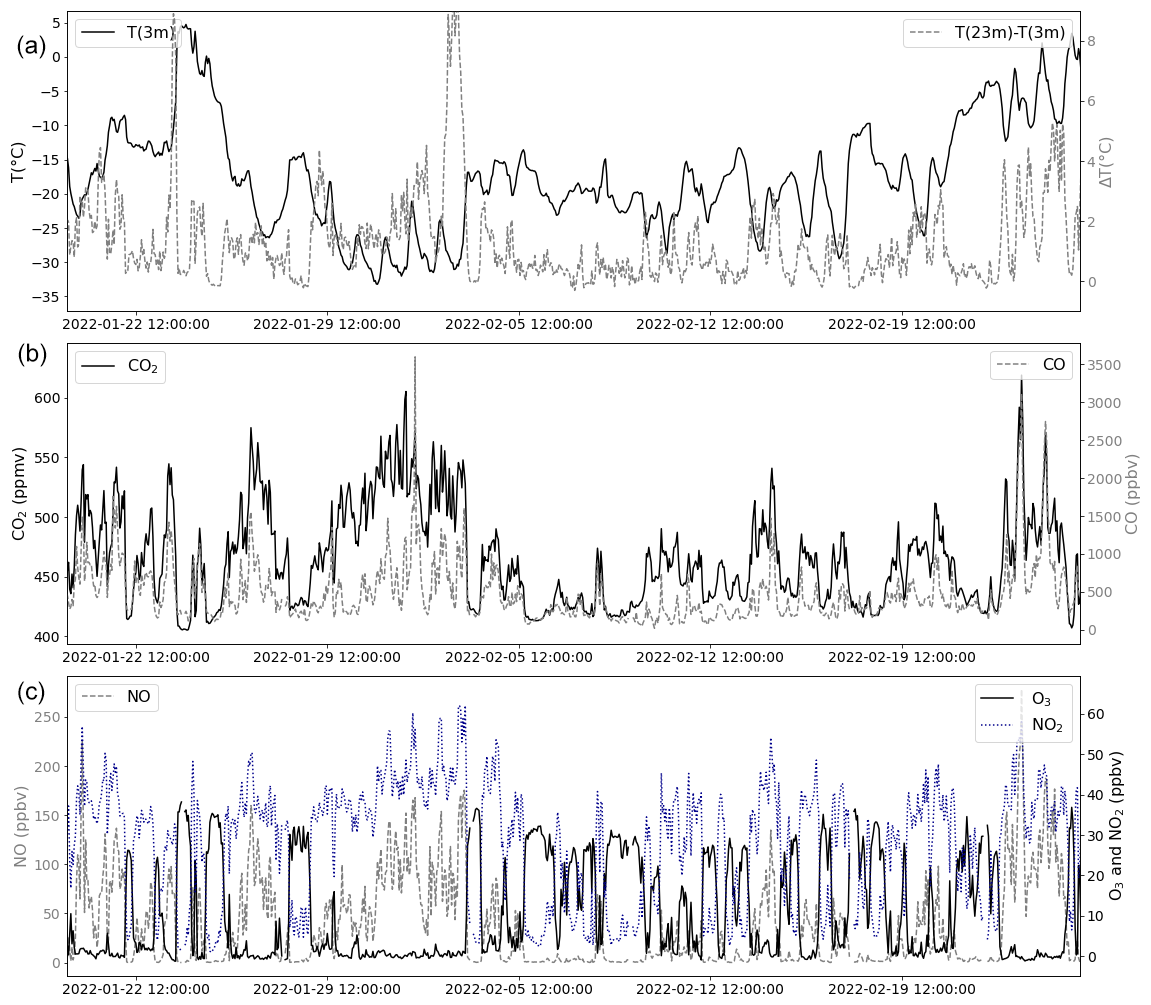
Figure 1 Time series of hourly averaged CTC measurements. (a) Temperature at 3 m (red; left axis) and T(23 m)–T(3 m) (dashed grey line; right axis). (b) CO₂ (solid black line; left axis) and CO (dashed grey line; right axis). (c) NO (dashed grey line; left axis), NO₂ (dotted blue line; right axis), and O₃ (solid black line; right axis).

The trace gas concentrations at the CTC are therefore highly variable, depending on the local meteorological conditions. This was taken into account when choosing the learning and prediction datasets, notably the concentration ranges, to perform and validate the calibration of the EGSs.

2.4 MICROMEGAS deployment strategy

During the ALPACA 2022 field experiment, the MICROMEGAS instrument was deployed in three different ways. It was operated at the CTC site for calibration against reference analysers for seven periods corresponding to a total of 250 h (see Fig. 2). At the CTC, the temperature recorded on one of the EGSs (see Fig. 3) displays a moderate variability (11 to 28 °C) compared to the outside temperature, which varies from −34 to 5 °C (see Fig. 1). According to their data sheets, the A4 sensors can be operated over a wide range of temperatures from −30 to 50 °C for NO, NO₂, and CO and −20 to 50 °C for O_x (https://www.alphasense.com/, last access: 24 February 2025). The thermal regulation of the sensors limits the effect of outside temperature variations on the measured concentrations. Nonetheless, this effect is accounted for when calibrating the data, as described in Sect. 2.5. The outside air RH sampled by the MICROMEGAS SHT75 sensor varies between 28 % and 83 %, with the lowest values recorded during the coldest period from 29 January to 3 February.

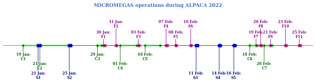
Figure 2 Timeline of MICROMEGAS operations during ALPACA 2022 with (green; C1 to C7) calibration periods at the CTC site, (red; F1 to F11) flights on board the helikite at the UAF farm site, and (blue; S1 to S7) car (“Sniffer”) rounds on board road vehicles.

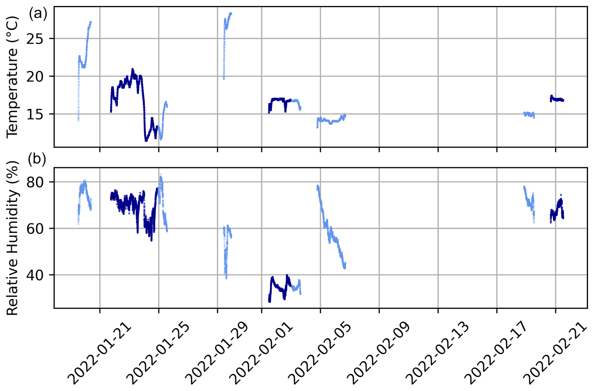
Figure 3 Time series of the (a) temperature of EGSs for learning (light blue) and prediction (dark blue) periods. (b) Relative humidity (RH) of air sampled by the EGSs.

MICROMEGAS was also deployed five times between 21 January and 16 February in a vehicle for the surface mapping of pollution in and around Fairbanks. The MICROMEGAS insulated box was placed inside a larger plastic box on the roof of the vehicle. The vehicle was driven at a speed slower than 20 m h⁻¹ in order to sample distances shorter than 500 m min⁻¹. It also stopped frequently for a few minutes to sample specific locations.

Finally, MICROMEGAS was incorporated in the MoMuCAMS platform to be deployed with other instruments on board the helikite at the UAF farm site. The balloon payload was designed to sample vertical profiles of trace gases and particles and possibly intercept pollution plumes in the ABL. The MICROMEGAS instrument weighs only 2 kg. It could therefore replace the MoMuCAMS CO and O₃ instruments for less than half their combined weight to save space and weight in order to fly with a more complete aerosol package (see Pohorsky et al., 2024b). More importantly, it also measures NO and NO₂, which are not part of the MoMuCAMS instrumental package. MICROMEGAS performed 11 successful balloon flights. Nighttime flights reached higher altitudes (up to 350 m a.g.l.) and lasted longer (up to 5 h) than daytime flights because of air traffic regulations.

Data from the MoMuCAMS CO and O₃ instruments were compared to the calibrated MICROMEGAS observations when the instruments were jointly operated at the UAF farm site (Sect. 3.2.1) and during helikite flights (Sect. 3.2.2).

2.5 Calibration methodology

As mentioned in the Introduction, low-cost EGSs calibration can be conducted under controlled atmospheric conditions (gas concentrations, temperature, and humidity) in laboratories or ambient conditions in the field. The latter option allows the sampling of more realistic conditions that better match the environmental conditions encountered during observations. Furthermore, during the ALPACA-2022 campaign, we had observations with reference analysers for four target gases (CO, O₃, NO, and NO₂) at the CTC site. We have therefore chosen the second option for our calibration.

2.5.1 Regression method

The calibration methods themselves fall into two categories, namely parametric and non-parametric methods. Many studies use parametric ML methods that simplify the function to be fit to a known form. The simplest forms are univariate or multivariate linear or quadratic functions which are often used as reference methods (Spinelle et al., 2015, 2017; Bigi et al., 2018; Casey et al., 2019; Malings et al., 2019; Liang et al., 2021; Bittner et al., 2022). The calibration model from the manufacturer, called “raw” in the paper, is based on a linear regression (LR) between calibrated gas concentrations and the voltages output by the electrodes of the sensors.

More sophisticated forms could be artificial neural networks (ANNs; Casey et al., 2019; Malings et al., 2019; Spinelle et al., 2015, 2017). Non-parametric ML algorithms have also been used such as decision trees (Bigi et al., 2018; Smith et al., 2019), support vector machines (Bigi et al., 2018), Gaussian processes (Smith et al., 2019; Malings et al., 2019), or k nearest-neighbour clustering (Malings et al., 2019; Bittner et al., 2022). To take advantage of parametric and non-parametric methods, some authors have also developed hybrid models combining, for instance, linear regression and random forest (Zauli-Sajani et al., 2021; Zimmerman et al., 2018; Malings et al., 2019; Bittner et al., 2022).

Parametric and non-parametric methods have their advantages and drawbacks. Non-parametric methods generally provide better fits than parametric methods because the form of the relationship between the EGS gas concentrations (output) and input parameters (working and auxiliary electrode voltages, humidity, and temperature) is less constrained. Nevertheless, they have difficulties for prediction in conditions (target or interfering gas concentrations, temperature, or humidity) that fall outside of the learning dataset. In contrast, parametric models generally allow broader and more reliable extrapolations to conditions outside of those of the learning dataset. However, they are subject to a lower flexibility of the input–output relationships, which are set to a given function or set of functions.

Spinelle et al. (2015) (respectively, Spinelle et al., 2017) proposed LR or multivariate linear regressions (MLRs) and ANN methods for the calibration of O₃ and NO₂ (respectively, NO, CO, and CO₂) sensors. As they concluded that simple LRs and MLRs are characterized by high uncertainties, we tested the MLR and slightly different linear methods. LR minimizes a difference in order to reproduce best a mean value. Quantile regressions (QRs) allow us to minimize the differences to best reproduce a given quantile (q) such as the median (q = 0.5). We therefore tested QR methods with q = 0.25 (QR0.25), 0.5 (QR0.5), and 0.75(QR0.75).

Spinelle et al. (2015) also used two types of ANNs, namely radial-based functions and a multi-layer perceptron (MLP). They found out that the former did not yield satisfactory results and thus discarded it. Spinelle et al. (2015, 2017) relied on MLPs because they provided very good results. Following their recommendations, we tested calibrations with a MLP. The MLP is a supervised learning algorithm that requires tuning multiple hyperparameters to achieve optimal results. After preliminary tests varying these hyperparameters, the results of the MLP calibration were not found to be very sensitive to the number of neurons, layers, and iterations that we set to 10, 10, and 4000, respectively. The results appeared more sensitive to the regularization parameter α (introduced to mitigate overfitting). Large α values promote smaller weights, thus improving the fit for high variances but potentially leading to overfitting; lower α values favour larger weights and, hence, better fix high biases, which may result in underfitting. Based on our preliminary tests, we present the best results which were achieved with α between 1 and 1000.

Non-parametric methods such as random forest (RF) are also used for EGS calibration (Bigi et al., 2018; Smith et al., 2019). We tested two renowned ensemble non-parametric methods, namely the histogram-based gradient-boosting trees (HGBT) and the RF. The RF model is set with 100 estimators (trees in the forest), with 5 samples required to be at a leaf node and a minimum of 2 samples required to split an internal node. The HGBT model has a maximum number of iterations of the boosting process (maximum number of trees) set to 100 and a maximum number of leaves for each tree set to 15. Our calibration ML tools are based on Python libraries from the scikit-learn initiative (https://scikit-learn.org/stable/, last access: 24 February 2025) described in Pedregosa et al. (2011).

To select the most robust method, the calibration data had to be split into two parts, with one for the learning of the calibration functions (Eq. 1 below) and one to validate the predictions made by these functions. The use of randomly selected training and prediction data yields excellent results, with Pearson correlation coefficients (R) generally exceeding 0.95 for the training and prediction data. The fact that the performances of the different models are almost identical, as are the results obtained from the training and prediction data, does not allow selecting the best model with this random choice of prediction data. Furthermore, when the trained models are applied to balloon data, some of them produce inconsistent results such as constant gas concentrations during portions of the flights and abrupt transitions from one constant value to another. This is particularly true for the non-parametric methods, namely RF and HGBT, which struggle to extrapolate beyond the training dataset. Indeed, during balloon flights, weather conditions and especially pollution levels differ from those encountered in the city at the CTC site. In order to overcome those difficulties, the CTC data were split into two equal and independent parts of ∼ 125 h (see Fig. 3), with both containing very cold and highly polluted periods and warmer and less polluted periods. The choice of two independent subsets instead of a validation set randomly selected from the whole dataset allows us to test methods more robustly, particularly their ability to extrapolate when conditions fall outside the training set limits, as will be presented in Sect. 3.1.

The pollution levels of the learning and prediction periods can clearly be inferred from NO levels in Fig. 7. It has to be noted that the learning and prediction periods were identical for the four gases.

2.5.2 Regression parameters

As mentioned earlier, the output voltages of the EGS depend not only on the concentration of the target gas but also on that of interfering gases, as well as RH and temperature (T). Therefore the calibration function f to be adjusted must be a function of all these parameters. As we do not have direct measurements of the interfering gases, we use the voltage of the working electrode V_w and of the auxiliary electrode V_a of the EGS targeting these gases when available. For the EGS targeting gas G0 with cross-sensitivities to gases G(i) with i = 1 to n, the generic calibration function can be written as

$$\begin{array}{}\text{(1)}& \begin{array}{rl}\left[G\mathrm{0}\right]=f(& V_{\mathrm{w}}\left(G\mathrm{0}\right),V_{\mathrm{a}}\left(G\mathrm{0}\right),V_{\mathrm{w}}\left(G\right(\mathrm{1}\left)\right),V_{\mathrm{a}}\left(G\right(\mathrm{1}\left)\right),\mathrm{\dots },\\ & V_{\mathrm{w}}\left(G\right(n\left)\right),V_{\mathrm{a}}\left(G\right(n\left)\right),\text{RH},T).\end{array}\end{array}$$

According to its data sheet from Alphasense, the CO-A4 EGS does not present important cross-sensitivities to other trace gases. Furthermore, Liang et al. (2021) do not use interfering gases for the calibration of CO-B4 Alphasense sensors in monitoring AQ in Chinese cities. Therefore, no interfering gases are introduced in the calibration function (Eq. 1) for CO.

With laboratory measurements, Lewis et al. (2016) showed that for Alphasense B4 EGS the working electrode of O_x sensors is equally sensitive to O₃ and NO₂, the electrode of NO sensors to NO and NO₂, and the electrode of NO₂ sensors mostly sensitive to NO₂ and less sensitive to NO. Some regression models for NO and NO₂ include the net (V_w−V_a) voltages from the NO and NO₂ sensors (Bigi et al., 2018). Based on these studies with varying approaches, we performed sensitivity tests with various combinations of trace gases for the NO, NO₂, and O_x sensors. For NO, the addition of the NO₂ voltage as a variable in its calibration function makes no significant difference, and no interfering gases are accounted for in the NO regression. For NO₂, the addition of voltages from the NO sensor in Eq. (1) slightly improves the agreement with the reference data, and therefore NO is accounted for in the NO₂ regression as a cross-sensitive gas. For O₃, the best results are obtained with the addition of the voltages of the NO₂ and also of the NO sensor.

2.5.3 Evaluation statistics

To choose the best calibration method for each trace gas, it is necessary to evaluate how the fit obtained with each method reproduces the reference data in terms of absolute value (accuracy) and variability (precision). The accuracy (systematic error) is quantified by the mean bias error (MBE) (i.e. average difference between the reference and the calibrated data); the precision or average magnitude of the errors is approximated by the root mean square error (RMSE) (i.e. the square root of the average of the squared differences between reference and calibrated data). The agreement regarding the phase of the variations can be assessed with the Pearson correlation coefficient R. The agreement regarding the amplitude of the variations can be evaluated with the ratio between the standard deviation of the calibrated data and that of the reference data.

The Taylor diagram, commonly used in meteorology and climate science, takes advantage of the trigonometric relationship between the RMSE, standard deviations, and correlation coefficients to synthetically display the performances of multiple datasets against a reference dataset (Taylor, 2001). It consists of a circular grid, with each dataset represented by a point and with the reference dataset placed at the centre of the x axis (e.g. see Fig. 4). The distance between a data point and the reference point provides the RMSE of the experiment, and the distance from the centre of the diagram provides the ratio of the standard deviations. The correlation coefficient between the reference and the experiment is given by the azimuthal position of the point. For each experiment, the RMSEs and standard deviations are normalized by the standard deviation of the reference data to display the results from multiple experiments on a single diagram.

3 Results

3.1 Validation against reference measurements

For comparison with reference data at the CTC site, MICROMEGAS data were averaged in 1 min intervals. For the four trace gases, the correlation coefficient R, MBE, and RMSE from comparisons between MICROMEGAS-calibrated data and reference learning and prediction data at the CTC are gathered in Table 1 for the selected calibration methods. We also provide the slope of the linear regressions fitted between MICROMEGAS and reference data.

Table 1 Statistics of the comparisons between MICROMEGAS and reference data at the CTC, including the correlation coefficients (R), mean bias error (MBE), root mean square error (RMSE), and slope of the regression line fitted (MICROMEGAS versus reference) between both datasets.

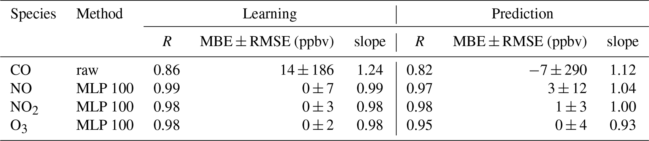
The choice of the calibration method for each target trace gas is explained in the following subsections which present the detailed calibration results for CO (Sect. 3.1.1), NO (Sect. 3.1.2), NO₂ (Sect. 3.1.3), and O₃ (Sect. 3.1.4).

3.1.1 CO

The Taylor diagram of the CO sensor displays the results from the different calibration methods for the learning and prediction datasets at the CTC (Fig. 4a). As expected, the performances are better for the learning dataset than for the prediction dataset, with larger correlation coefficients (0.86 < R < 0.96 for learning and 0.74 < R < 0.83 for prediction) and ratios of variabilities relative to the reference data closer to unity. The HGBT and RF achieve the best agreement for learning but almost the worst for prediction. These non-parametric methods are characterized by a strong flexibility that enable them to match the reference dataset very well, but they have difficulties with predicting data that fall even slightly outside of their learning database. In our case, learning and prediction datasets are chosen within periods with similar weather and pollution conditions but with some differences that are probably the reason for the lower performances with the prediction dataset.

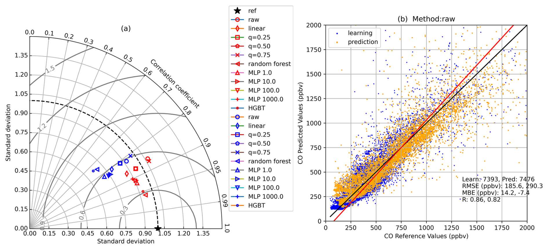
Figure 4 CO calibration methods. (a) Taylor diagram for MICROMEGAS versus CTC reference measurements with (red symbols) learning data and (blue symbols) prediction data. (b) Scatter plot of MICROMEGAS raw data versus CTC with (orange symbols) learning data and (blue symbols) prediction data, together with the (black line) unity and (red line) linear regression.

Except for the non-parametric methods, all the calibration methods have R values slightly larger than 0.8 for the prediction dataset (Fig. 4a). The differences come from their ability to reproduce the amplitude of the CO variability from the reference dataset, with ratios varying from 0.71 (MLP1.0) to 0.97 (QR0.75). The performances of the raw data in reproducing the variability in the reference data are almost similar to the performances of QR0.75, but the raw data MBE is much smaller, at −7 instead of 61 ppbv (see Table 1), and we have therefore chosen to use the raw data for the CO EGS.

The time series of CO measurements (raw data) from MICROMEGAS and the reference CO analyser are displayed in Fig. 5. MICROMEGAS captures well the very large CO variations from hundreds to thousands of ppbv. However, the absolute biases can reach 1 ppmv for the highest concentrations. As a result, the absolute RMSE between the reference and MICROMEGAS CO data for the prediction dataset is rather large (290 ppbv).

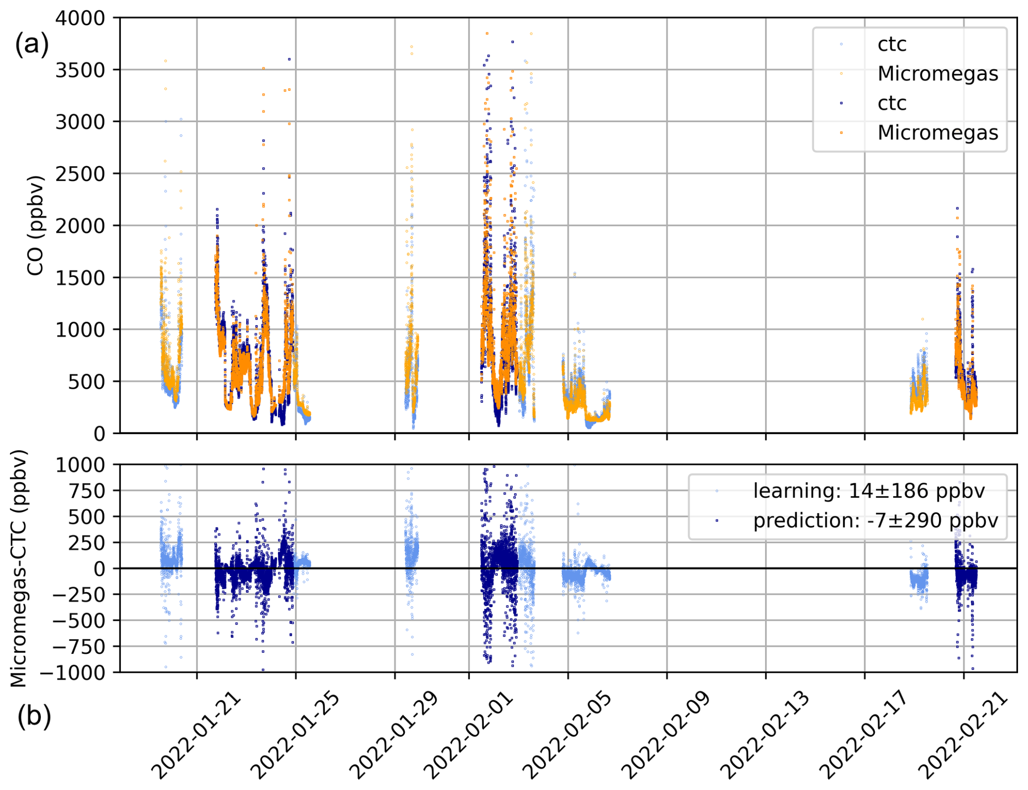
Figure 5 (a) Time series of CO measurements (raw data) at the CTC site (blue symbols) reference analyser data (orange symbols) MICROMEGAS data. Learning data are in light colours and prediction data in dark colours. (b) Time series of the differences between the MICROMEGAS and the reference analyser data for (light blue symbols) learning data and (dark blue symbols) prediction data.

3.1.2 NO

The NO Taylor diagram (Fig. 6a) differs greatly from the CO one. All the experiments have correlation coefficients R > 0.9, and the majority of them are even larger than 0.95. The variabilities in the MICROMEGAS experiments are mostly in the range 0.90–1.05 times the variabilities in the reference data, and the RMSEs are lower than 30 % of the reference data variability. We have chosen the MLP100 method because it displays the largest R and a variability ratio of 1.0. Furthermore, the slope of the linear regression between the reference and MICROMEGAS data is very close to unity (Fig. 6b and Table 1), with only a very limited number of negative MICROMEGAS NO values which do not exceed a couple of ppbv (Fig. 6b).

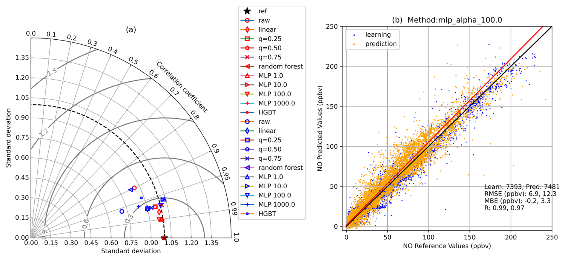
Figure 6 NO calibration methods. (a) Taylor diagram for MICROMEGAS versus CTC reference measurements with (red symbols) learning data and (blue symbols) prediction data. (b) Scatter plot of MICROMEGAS MLP-100 data versus CTC with (orange symbols) learning data and (blue symbols) prediction data, together with the (black line) unity and (red line) linear regression.

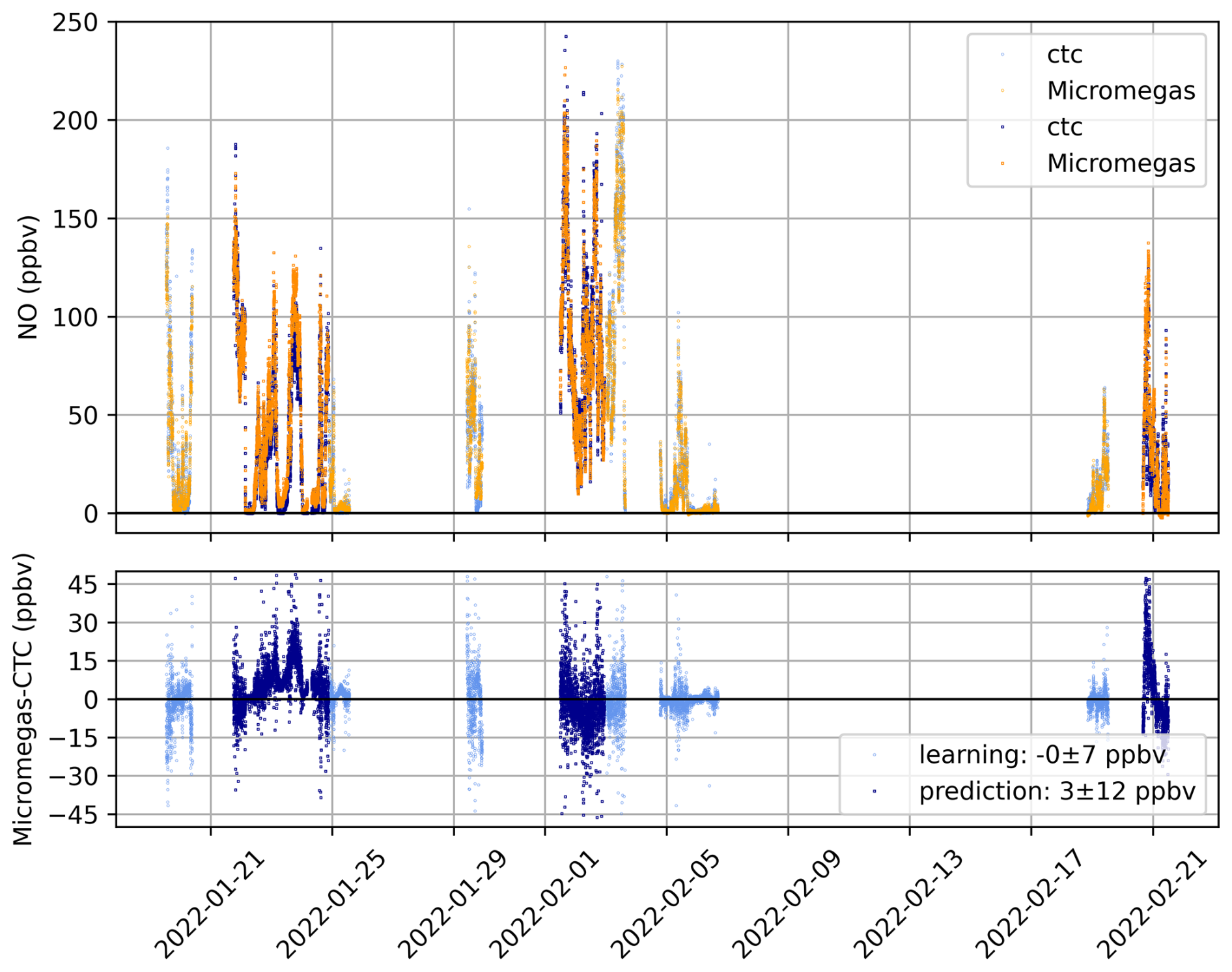
The ability of MICROMEGAS to capture the NO large variability (0–250 ppbv) is illustrated by the time series at the CTC displayed in Fig. 7. The discrepancies are larger for the prediction than for the learning dataset, with biases reaching ±50 and ±30 ppbv, respectively. Nevertheless, the global RMSE for prediction remains moderate at 12 ppbv, and the MBE of 3 ppbv is not significant.

Figure 7 Same caption as Fig. 5 but for NO (MLP100 calibration function).

3.1.3 NO₂

The NO₂ Taylor diagram is very similar to the NO one (Fig. 8a). Most experiments have R > 0.95, and variability ratios are even closer to unity than for NO. For the prediction, most experiments provide very similar results. We have chosen MLP100, which performs slightly better than MLP1 or MLP10. Even if they are able to reproduce the variability in the reference data correctly, linear regressions are excluded because, contrary to MLP, they provide significantly negative values. The raw calibration method displays a good correlation with the reference data but only just half of its variability.

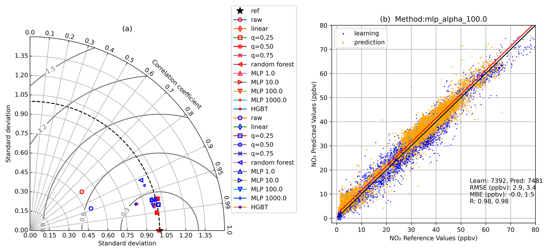
Figure 8 NO₂ calibration methods. (a) Taylor diagram for MICROMEGAS versus CTC reference measurements with (red symbols) learning data and (blue symbols) prediction data. (b) Scatter plot of MICROMEGAS MLP-100 data versus CTC with (orange symbols) learning data and (blue symbols) prediction data, together with the (black line) unity and (red line) linear regression.

The scatter plot between MICROMEGAS and reference NO₂ data (Fig. 8b) shows excellent agreement with a linear regression slope of unity.

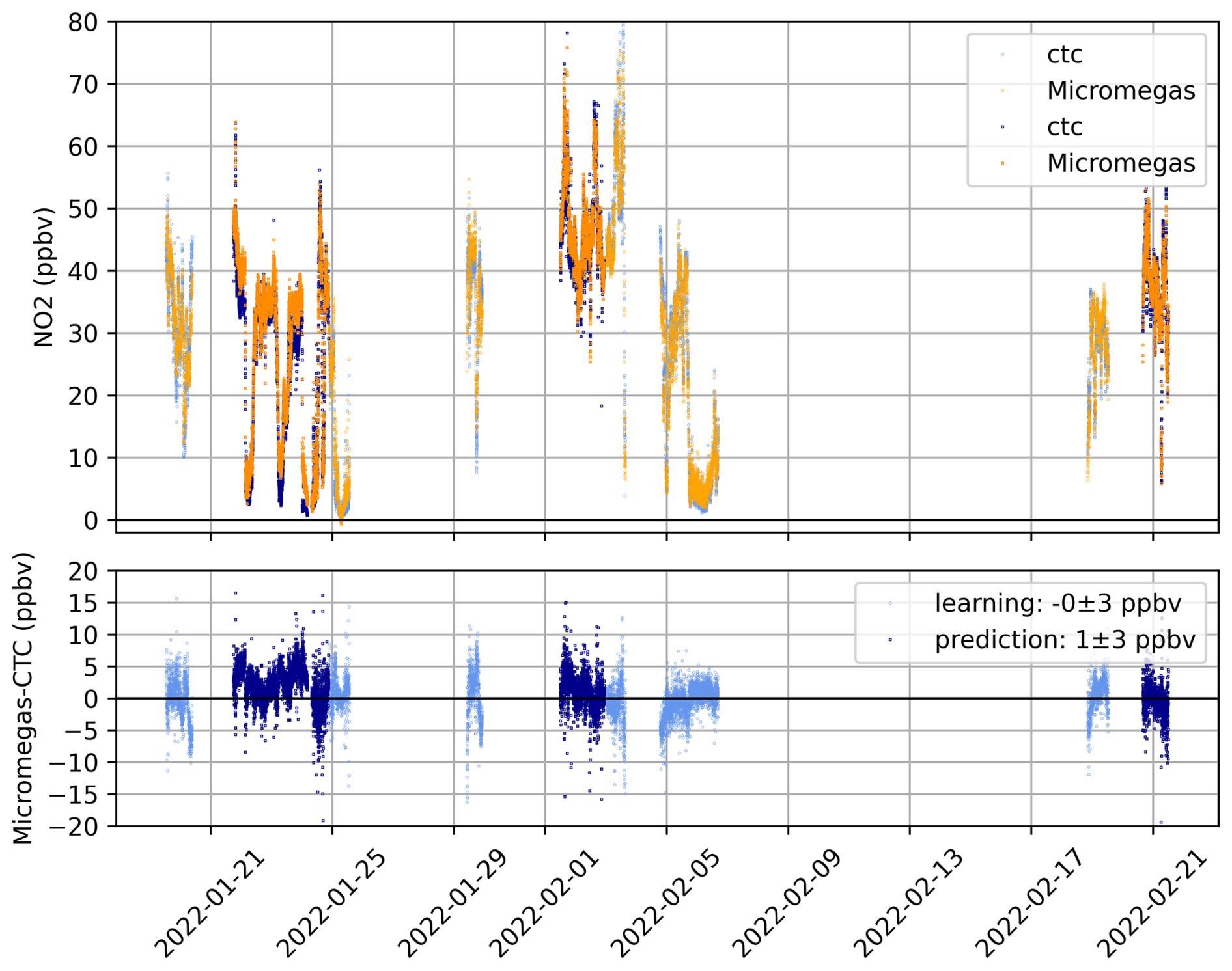
As expected from the previous analysis, MICROMEGAS data closely follow the NO₂ variations from the reference analyser (Fig. 9). The difference between both datasets is within ±10 ppbv (95th percentile), with a very low mean bias (1.5 ppbv), and the RMSE (3 ppbv) is about 4 times lower than for NO.

Figure 9 Same caption as Fig. 5 but for NO₂ (MLP100 calibration function).

3.1.4 O₃

For O₃, the prediction results are characterized by decreased performances relative to the learning results and to the NO₂ prediction results (Fig. 10a). The best calibration method is clearly MLP100, with a correlation coefficient of 0.95 and an amplitude of variability that is only 10 % lower than that of the reference. The scatter plot displays the bimodal O₃ distribution with low values (< 5 ppbv) from an almost complete O₃ titration by NO during high-pollution periods, and O₃ between 20 and 40 ppbv during cleaner periods. The linear regression slope (0.93) is lower than for the other gases (Table 1) but remains quite close to unity. The MLP100-calibrated O₃ data are never negative, contrary to O₃ from linear calibration methods.

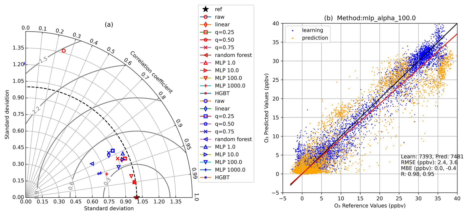
Figure 10 O₃ calibration methods. (a) Taylor diagram for MICROMEGAS versus CTC reference measurements with (red symbols) learning data and (blue symbols) prediction data. (b) Scatter plot of MICROMEGAS MLP-100 data versus CTC with (orange symbols) learning data and (blue symbols) prediction data, together with the (black line) unity and (red line) linear regression.

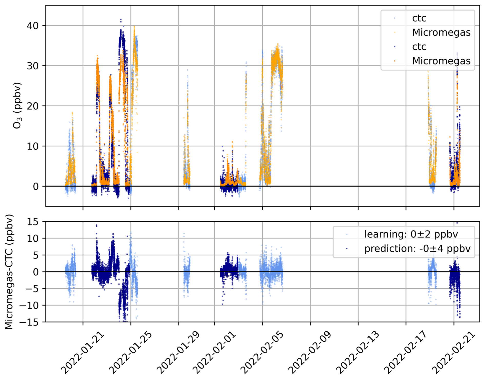
MICROMEGAS O₃ captures the variations in the reference O₃ (Fig. 11) with the alternance of polluted periods with little O₃ and cleaner periods with about 30 ppbv of O₃ in anti-correlation with the NO levels (Fig. 7). For the prediction dataset, biases can reach absolute values larger than 10 ppbv for the highest levels of O₃ but the mean bias is 0 ± 4 ppbv.

Figure 11 Same caption as Fig. 5 but for O₃ (MLP100 calibration function).

3.2 Comparisons of CO and O₃ from MICROMEGAS to analysers from MoMuCAMS

3.2.1 At the UAF farm site on the ground

MICROMEGAS was operated on the ground at the UAF farm site before the helikite flights or between two successive flights for five periods of hours to days. When they were not flying, CO and O₃ MoMuCAMS instruments (see Sect. 2) were also operated at the UAF farm site. The MoMuCAMS CO PICO (respectively, O₃ 2B Tech) instrument was operated for 129 h (respectively, 105 h) in coincidence with MICROMEGAS at the site. The results from comparisons between the CO and O₃ instruments are displayed in Figs. 12 and 13, respectively, and the corresponding statistics are presented in Table 2.

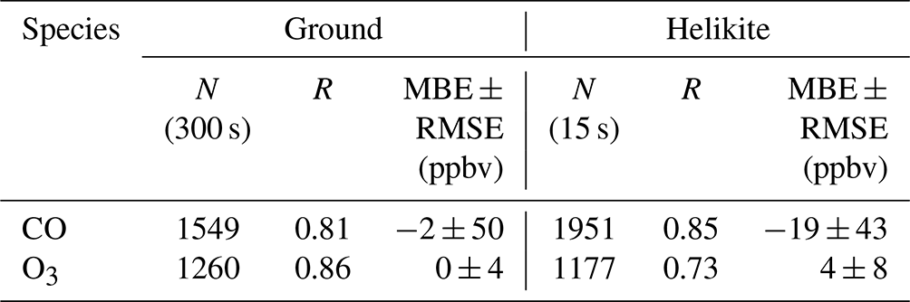
Table 2 Statistics of the comparisons between MICROMEGAS and MoMuCAMS analysers CO and O₃ data at the UAF farm site and on board helikite, including the correlation coefficient (R), mean bias error (MBE), root mean square error (RMSE), and ratio of MICROMEGAS on analyser standard deviations. N stands for the number of data points. Data were averaged for 300 s periods on the ground and 15 s on board helikite.

The UAF farm site at the edge of the city is less polluted than the CTC site downtown. The CO concentrations remain within the 100–300 ppbv range (Fig. 12), while CO concentrations at the CTC are mostly over 500 ppbv and often exceed 1 ppmv (see Fig. 1). At the UAF farm, O₃ is seldom fully titrated by NO, with concentrations mostly between 20 and 40 ppbv and below 10 ppbv over rare and short periods (Fig. 13). This is in contrast with the CTC, where O₃ is fully titrated by NO over several periods that can last many days (Fig. 1).

CO from MICROMEGAS has no systematic bias (−2 ± 50 ppbv) relative to the PICO instrument. The RMSE (50 ppbv) is much lower than at the CTC because the absolute CO values are much lower. According to Fig. 12, the absolute differences between both instruments rarely exceeds 50 ppbv. The correlation coefficient (R = 0.81) between MICROMEGAS and PICO CO data at the UAF farm is very close to the one for the CO prediction data at the CTC (Table 1).

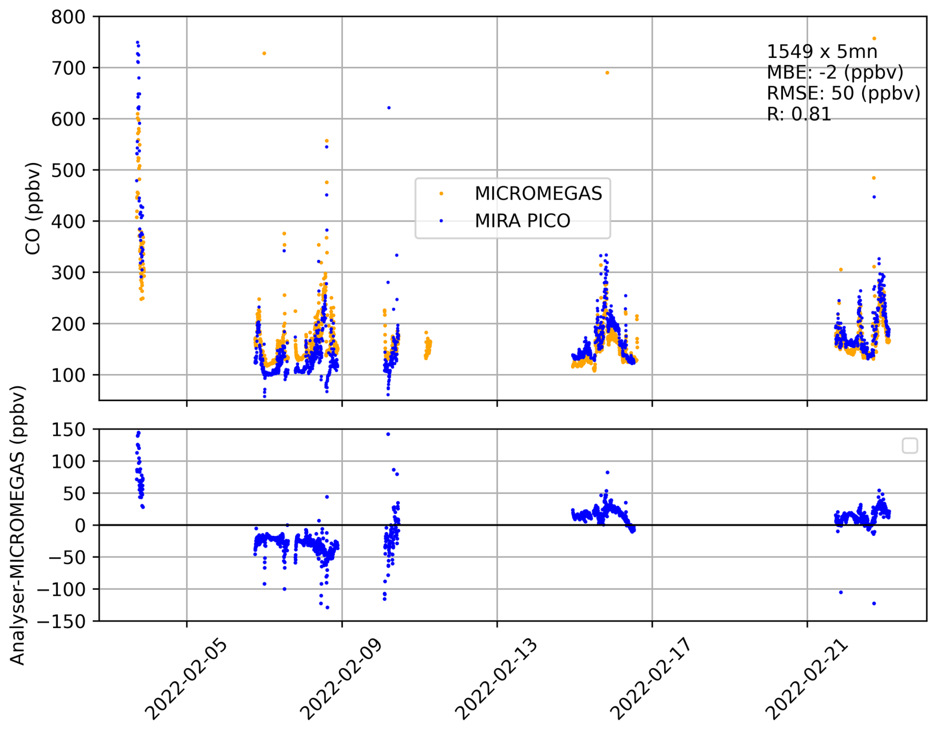
Figure 12 Time series of CO measurements at the UAF farm site, with (orange symbols) MICROMEGAS data and (blue symbols) MoMuCAMS analyser (MIRA PICO) data. The differences (“Analyser–MICROMEGAS”) are displayed in the bottom panel.

For O₃, no systematic bias (0 ± 4 ppbv) is observed between MICROMEGAS and the 2B Tech instrument. Moreover, the MBE (0 ppbv) and RMSE (4 ppbv) are identical to those computed for the prediction dataset at the CTC (Table 1). The correlation coefficient (R = 0.86) is nonetheless lower than at the CTC (Table 1). This is probably related to the O₃ variability, which is lower at the UAF farm with no complete O₃ titration and only few periods with low-O₃ concentrations.

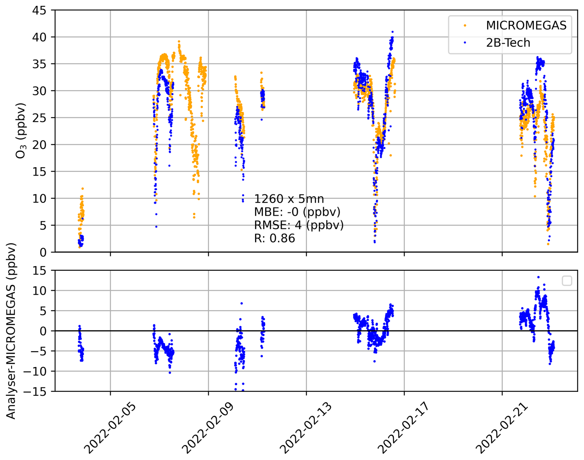
Figure 13 Time series of O₃ measurements at the UAF farm site with (orange symbols) MICROMEGAS data and (blue symbols) MoMuCAMS analyser (2B Tech) data. The differences (“Analyser–MICROMEGAS”) are displayed in the bottom panel.

3.2.2 On board the helikite

For a limited number of flights, MICROMEGAS was flown part of the time with the CO PICO or O₃ 2B Tech analysers and with both for one flight (23 February). The comparison dataset is more limited than at the ground with only 8 and 4 h of coincident measurements for CO and O₃, respectively. Despite the limited dataset and the significantly shorter averaging time compared to ground-based data (15 s versus 300 s), the statistics (see Table 2) remain very good, with even better agreement for CO. For O₃, the correlation coefficient (0.73) is noticeably lower than it was on the ground but remains acceptable, and the mean bias (4 ppbv) and RMSE (8 ppbv) are larger than at the ground. It is noteworthy that the averaging time for in-flight data is 20 times shorter, which results in increased noise and, consequently, a lower correlation coefficient and a larger RMSE.

The time series of CO and O₃ from MICROMEGAS and MoMuCAMS analyser data and flight altitudes for the flight of 23 February are displayed in Fig. 14. This flight is characterized by four ascents and descents between the ground and 120  m a.g.l. over a total duration of 2 h. Both types of instruments exhibit identical variations in CO and O₃, with a more polluted layer (high CO and low O₃) near the surface and background concentrations above the surface layer, resulting in high correlation coefficients between the datasets (0.97 for CO and 0.78 for O₃).

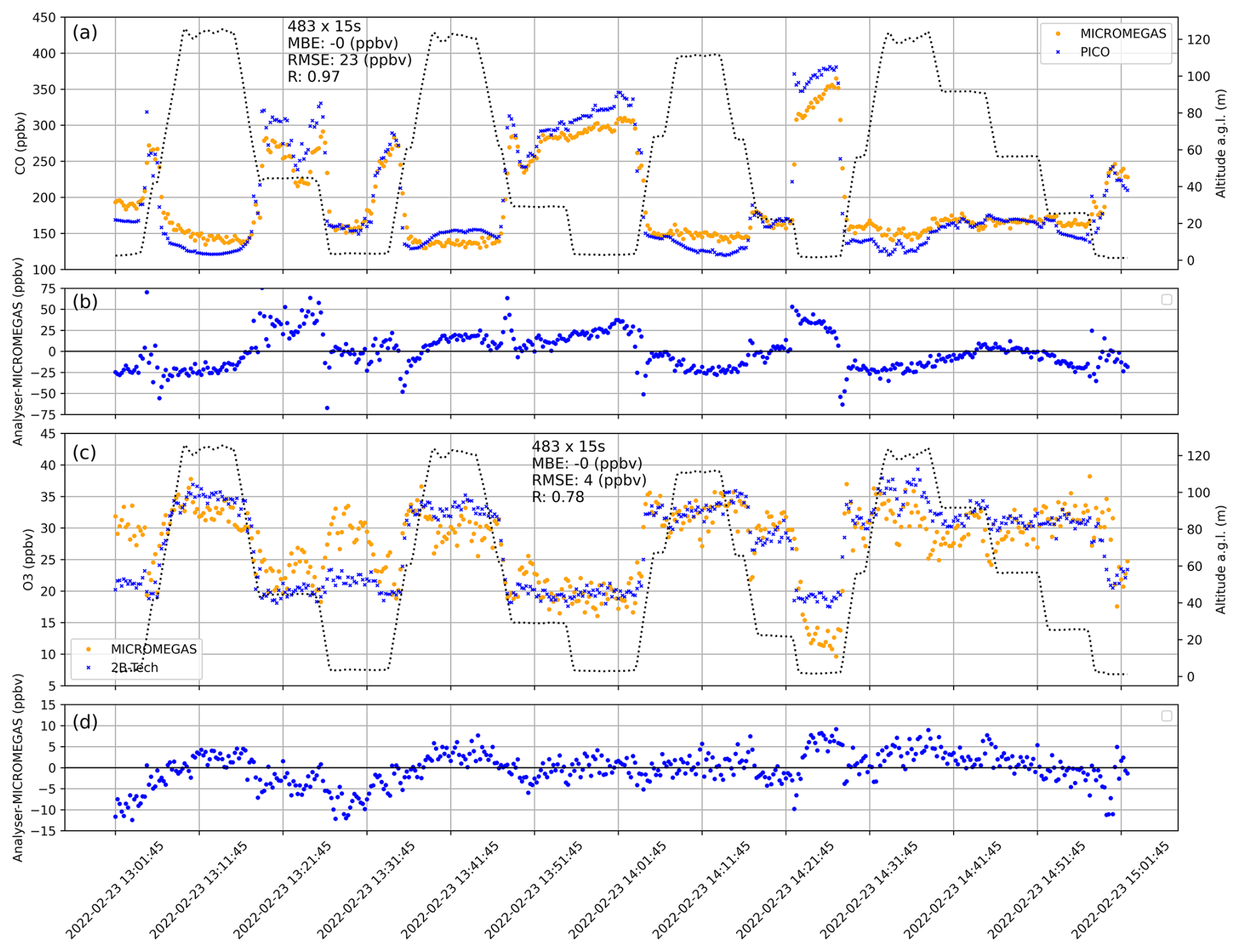
Figure 14 Time series of MICROMEGAS and MoMuCAMS measurements of CO in panel (a) and O₃ in panel (c) during the flight of 23 February with (orange symbols) MICROMEGAS data and (blue symbols) MoMuCAMS analyser data. The dotted black line on the right y axis represents the altitude of the balloon. The differences (“Analyser–MICROMEGAS”) are displayed in panel (b) for CO and panel (d) for O₃.

The comparison of in-flight data therefore shows that the EGS are not significantly impacted by the ascents and descents during the flights. The low vertical speed and limited-altitude excursion prevent variations in sensor behaviour during flights.

3.3 On-road mobile sampling

As mentioned in Sect. 2, MICROMEGAS was deployed 7 times on the roof of a vehicle to perform on-road mobile samplings in Fairbanks and its surroundings. We present here MICROMEGAS measurements from the first drive performed on 21 January from 12:39 to 16:40. The car was parked in a street next to the CTC measurement site at the start (12:39 to 13:09) and at the end (16:32 to 16:38) of the drive. The car first headed towards the residential neighbourhood of Hamilton Acres and stopped next to the instrumented site called The House. The next stop was at the Birch Hill Recreation Area. The car then headed west on College Road and reached the UAF farm site, after a stop at the Aurora residential area, and drove up to the top of Chena Ridge via Chena Ridge Road before descending towards Fairbanks Airport via Chena Pump Road. It then headed east on Parks Highway to reach the CTC site by going north (see Fig. 15).

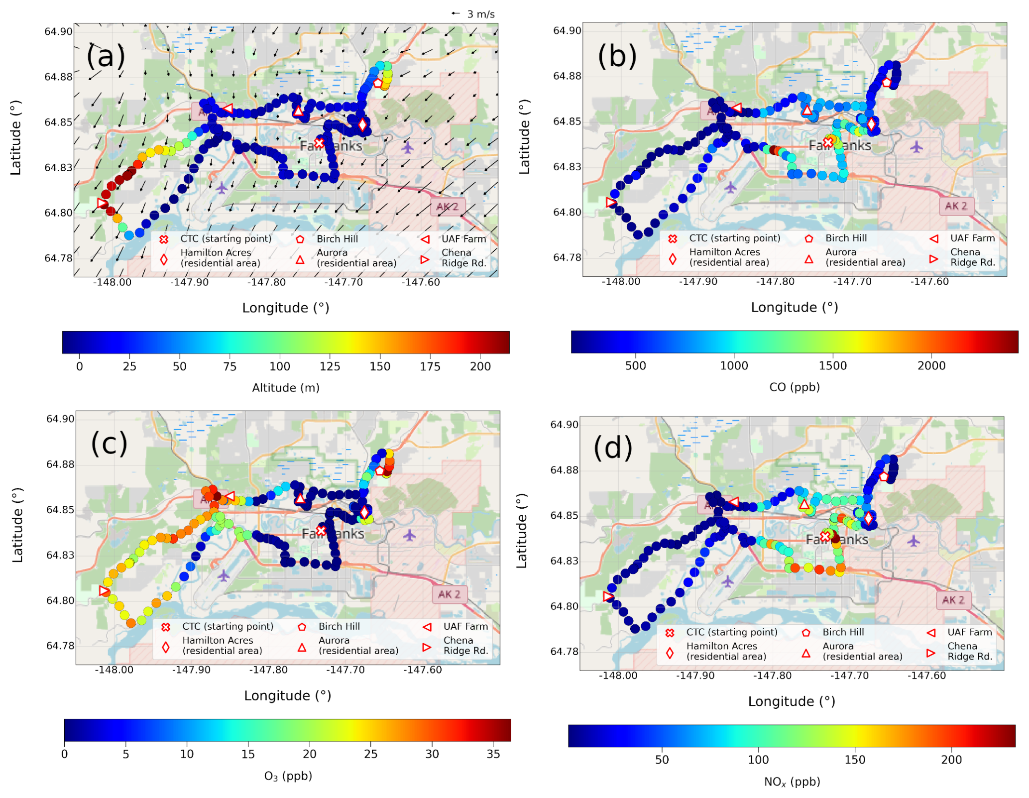
Figure 15 Maps with MICROMEGAS measurements from the drive of 21 January for (a) altitude with superimposed 0–10 m winds from the Weather Research and Forecasting (WRF) Model simulation (12:00–16:00 average). (b) CO, (c) O₃, and (d) NO_x. © OpenStreetMap contributors 2024. Distributed under the Open Data Commons Open Database License (ODbL) v1.0.

According to the CTC data (see Fig. 1), the period of the drive is characterized by relatively warm temperatures for the season (∼ −10 °C) and significant temperature inversions between 3 and 23 m altitude (between −2 and −1.5 °C). It is identified as strongly stable according to Brett et al. (2025), promoting elevated pollution levels. During the 4 h of the drive, the pollution levels increased at the CTC from 590 to 1610 ppbv for CO and from 40 to 110 ppbv for NO (see Fig. 16). Such increases probably result from the diurnal variability in road traffic.

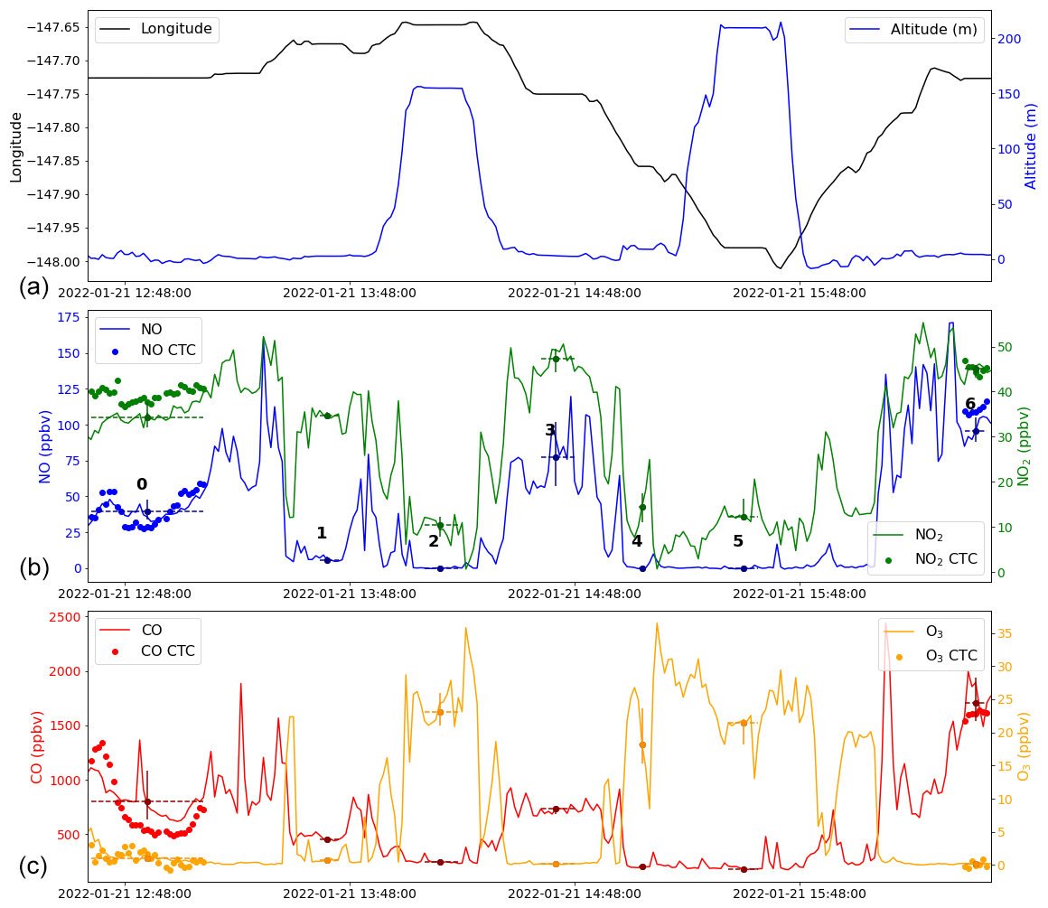
Figure 16 Time series of (a) longitude and altitude (b) NO and NO₂ and  (c) CO and O₃ for the drive of 21 January (minute averages). For each trace gas, the solid line corresponds to MICROMEGAS measurements, and full circles correspond to measurements from the reference analysers at the CTC for the two periods at the beginning and at the end of the drive when the car was parked in a street next to the CTC site. The full circles in darker colours correspond to the median MICROMEGAS values during the car stops. The horizontal dashed bars represent the duration of the stop and the vertical solid one the 10th–90th percentile range. The numbers on top of the NO line in the middle panel identify the stops as follows: (0) CTC, (1) Hamilton Acres, (2) Birch Hill, (3) Aurora, (4) UAF farm, (5) Chena Ridge, and (6) CTC.

The comparison between the CTC reference measurements and MICROMEGAS data (Fig. 16) clearly indicates that MICROMEGAS captures the variations in trace gas concentrations between the start and the end of the drive. It is noteworthy that MICROMEGAS is also able to capture the CO and NO variability very well for the half-hour at the CTC site before the car moves away. For O₃, the concentrations are close to zero during both stops at the CTC, and the agreement is excellent, with biases lower than 0.2 ppbv. MICROMEGAS slightly overestimates NO₂ (5.4 ppbv) at the beginning, and the bias decreases to 0.1 ppbv at the end. The NO bias is negligible at the start (−0.3 ppbv) and MICROMEGAS is underestimating NO by 14 ppbv at the end. For CO, the biases are larger at the beginning (210 ppbv) than at the end (101 ppbv). For the four trace gases, the biases are in good agreement with the intervals from Table 1. It has to be noted that at the beginning, MICROMEGAS sampled a peak with largely enhanced CO (and slightly enhanced NO) which was not detected by the reference analyser (Fig. 16). This discrepancy is most likely resulting from the location of MICROMEGAS on the roof of the car which was parked about 10 m away from the CTC trailer and closer to the traffic emissions than the analyser's inlet located on the roof of the trailer. Therefore, MICROMEGAS probably sampled a plume from the traffic that did not reach the analyser's inlet.

The pollutant maps of Fig. 15 display significant variations among the sampled areas. The first striking feature is that the O₃ concentrations (Fig. 15c) are strongly correlated with the altitude (Fig. 15a) on both uphill legs of the drive reaching Birch Hill to the northeast and Chena Ridge to the southwest. Elevated areas are indeed isolated from the strong emissions from the city, especially during temperature inversion periods. The background air sampled on the hill slopes is therefore also characterized by CO and NO_x concentrations lower than in the city. The large concentrations of NO_x and CO on the south leg of the drive from the airport to the CTC, following Airport Way and Parks and Richardson highways, are due to the sampling of air impacted by the traffic during the rush hours. NO_x concentrations are lower on the northern leg on Johansen Expressway and College Road, probably because of less traffic at the beginning of the afternoon.

The two residential areas sampled at 1 h intervals have different levels of pollutants. The Hamilton Acres area has a low level of NO (5 ppbv) and CO (450 ppbv) compared to the Aurora area, where NO reaches 77 ppbv and CO 730 ppbv (see Fig. 16). The levels of NO₂ are also larger at Aurora (47 ppbv) than at Hamilton Acres (35 ppbv). During the drive, at the beginning of the afternoon less traffic was seen in those residential areas. Nevertheless, at the Aurora site, the 0–10 m winds simulated by the WRF model (see Brett et al., 2025) are weak and blowing from the north, bringing air polluted by traffic on Johansen Highway to the residential area to the south. Stronger winds are blowing from the northeast (Fig. 16a), bringing clean air from outside of the city to Hamilton Acres. The differences in the wind strength and direction probably explain the difference in pollution levels between the two residential areas. The area around the UAF farm to the northwest of the airport is marked by enhanced O₃ and low-NO_x and CO concentrations as a result of the north flow bringing background air (Fig. 15a).

3.4 Vertical profiles from helikite flights

As mentioned earlier (Fig. 2), MICROMEGAS performed 11 helikite flights in the MoMuCAMS platform from 30 January to 25 February 2022. The helikite was operated as follows: the balloon made an initial ascent at maximum vertical speed (20 m min⁻¹) before descending in stages. Then, the cycle of ascents and descents is repeated several times. When a plume is detected (CO₂ and particles concentrations enhanced with respect to background concentrations), the balloon ascends and descends within the altitude range corresponding to this plume and makes prolonged stops of a few minutes around the altitude of maximum concentrations (see Pohorsky et al., 2024, for details). For the flights, MICROMEGAS data were averaged in 15 s bins corresponding to 5 m vertical displacement at maximum velocity.

The general statistics with the median values and the 95th, 80th, 20th, and 5th percentiles computed over the 11 flights are displayed in Fig. 17; Table 3 provides the median values and 20th and 80th percentiles computed over the whole dataset. For the four trace gases, the median values remain within relatively narrow ranges of values over the 0–350 m vertical range. Extreme values are particularly noticeable for NO₂, with peaks of up to 40 ppbv, 10 times larger than the median value and for O₃ with troughs down to 5 ppbv. Nevertheless, extreme values of CO, NO, and NO₂ observed during the flights remain low compared to what was observed at the CTC during long polluted episodes (Fig. 1). This is due to the location of the UAF farm, which is far from the large pollution sources and rather upwind of the dominant winds from the northern sector at Fairbanks.

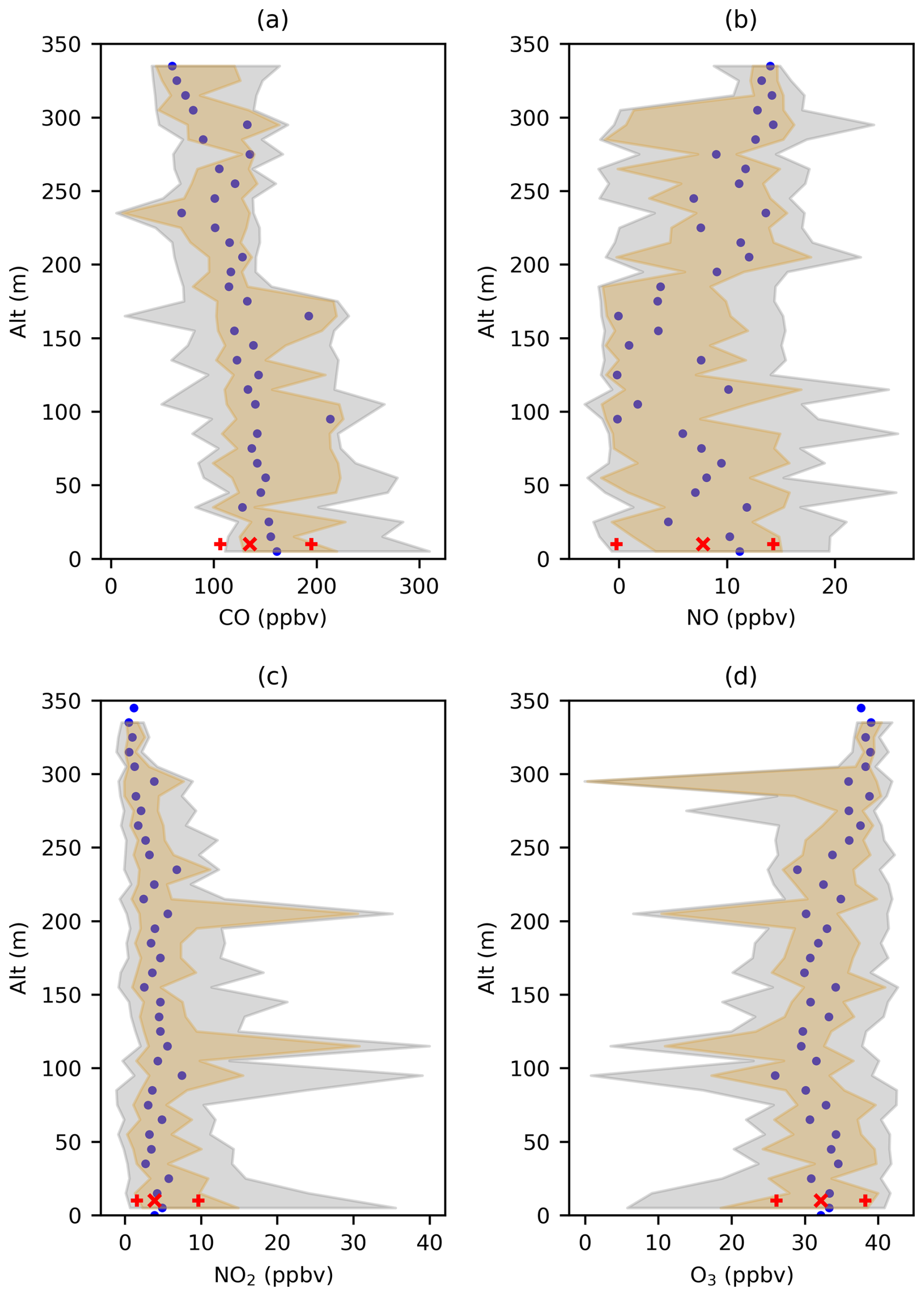
Figure 17 Statistics of the vertical profiles of CO, NO, NO₂, and O₃ (blue dots) median values. The orange shaded area shows the 20th–80th percentile range; grey shaded area shows the 5th–95th percentile range, with (red ×) the median value and (red +) 20th and 80th percentiles shown for the whole helikite profile dataset.

Table 3 Statistics (20th percentile, median, and 80th percentile) of the MICROMEGAS helikite data for the whole ALPACA-2022 campaign and for the flight of 20 February (numbers in parentheses).

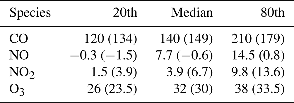
An example of a helikite flight with a plume detected on 30 January was given in Simpson et al. (2024). During that flight, peaks of NO₂ are recorded between 50 and 100 m and between 200 and 250 m, coincident with CO₂ enhancements. In Brett et al. (2025), MICROMEGAS NO_x and CO flight data were used to evaluate Lagrangian simulations of pollution plumes originating from power plants to the east of the UAF farm site and emitted aloft from elevated chimney stacks. They focused on the flights of 30 January and 8–9 and 25 February. Here, we present the data for the four trace gases (CO, NO, NO₂, and O₃) for the flight on the morning of 20 February when pollution plumes are detected aloft (Fig. 18). The origin of the pollution plume and the layering of the ABL during this flight are discussed in a separate on-going study. We focus here on the multispecies measurements of such a plume with the MICROMEGAS-calibrated data. The statistics over the whole flight are presented in Table 3. For CO, NO₂, and O₃, the median values are within the 20th–80th percentile ranges from the whole helikite datasets. The NO values on the flight are generally lower than the median value; nonetheless, this difference is still consistent with the evaluation of NO made in Sect. 3.1.2. Indeed, the mean bias between MICROMEGAS and the CTC reference data (3 ± 12 ppbv) encompasses the difference of −8.3 ppbv between the NO median of the whole helikite dataset and of the 20 February flight. The CO, NO₂, and O₃ values measured during the flight generally fall within the 20th–80th percentile from Table 3 but some extreme values are detected a few times at different altitudes. A plume located approximately between 120 and 180 m was sampled during three short periods (from 07:17 to 07:33, 09:54 to 10:11, and 10:46 to 10:59 AKST) during the flight. In the plume, CO and NO₂ concentrations reach maxima of, respectively, 417 and 46 ppbv, and O₃ decreases to 0 ppbv following titration. NO is enhanced with a maximum value of 11 ppbv in the plume but only clearly between 09:55 and 09:58. Finally, another plume is detected between 273 and 300 m from 09:22 to 09:33, with NO mixing ratios up to 27 ppb; it is correlated with O₃ titration but with very limited NO₂ and CO enhancements. According to the Lagrangian modelling of Brett et al. (2025), the plume at 150 m is originating from the UAF-C or Chena–Aurora power plant in Fairbanks, and the 285 m plume is not attributed.

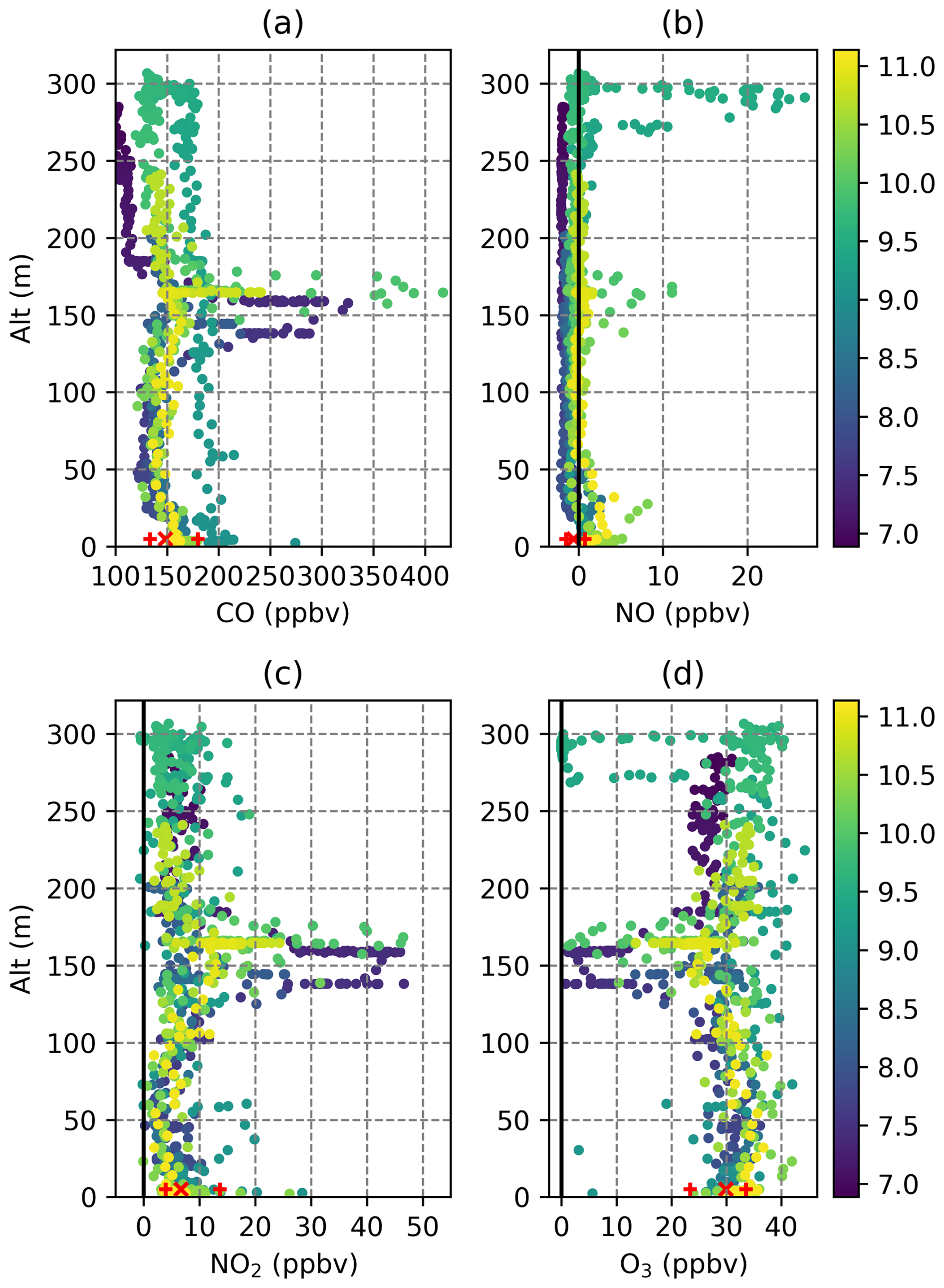
Figure 18 MICROMEGAS profiles of (a) CO, (b) NO, (c) NO₂, and (d) O₃ for the helikite flight on the morning of 20 February. The colours correspond to the hour (AKST) of observation since the start of the data acquisition, with the (red ×) median value and (red +) 20th and 80th percentiles for the whole flight.

4 Conclusions

The MICROMEGAS instrument has been successfully operated at Fairbanks, Alaska, during the ALPACA field experiment in January–February 2022 to sample surface distributions and vertical profiles of trace gases in the wintertime Arctic boundary layer. MICROMEGAS includes EGSs to measure NO, NO₂, O₃, and CO, as well as temperature and relative humidity sensors and a GPS for localization. It has been deployed on board a vehicle for seven on-road sampling drives in Fairbanks and the surroundings and at the UAF farm site to the northwest of Fairbanks on board a tethered balloon (the helikite) for 11 flights up to a maximum altitude of 350 m a.g.l. In order to calibrate and validate the EGSs, we also operated MICROMEGAS coincident with reference analysers at the instrumented CTC site downtown in Fairbanks for ∼ 250 h.

For the EGSs calibration, we have tested linear (quantile regressions) and non-linear (multi layer perceptron) parametric methods and also non-parametric (random forest and histogram-based gradient-boosting trees) methods. The use of Taylor diagrams allowed us to evaluate the ability of the different calibration methods to reproduce the variability from the reference data and to determine the optimal method. For CO, the linear relationship between the gas concentration and the sensor voltages provided by the manufacturer (raw method) provides the best agreement for prediction data, and we used no other calibration method. For NO, NO₂, and O₃, an excellent agreement was reached for the learning data with the non-parametric random forest method, but the performances are largely reduced for the predictions. The perfect learning is probably linked to the fact that non-parametric methods, such as random forest, are able to fit a large number of functional forms contrary to parametric methods which have fixed functional forms. The degraded results for the prediction results from the lower ability of the non-parametric methods to extrapolate outside of the learning database relative to parametric methods. The multivariate quantile regressions have correct performances concerning the reproduction of variabilities but provide too many negative values. This is due to the basic linear functional form that extrapolate to values which are outside of the reference data range. For NO, NO₂, and O₃, the best prediction results are obtained with multi-layer perceptron (MLP) artificial neural networks with 10 layers of 10 neurons when the network regularization parameter α is set to 100 (MLP100). The MLP parametric function is complex enough to reproduce the non-linear relationships between the different parameters and allows an extrapolation to reproduce data outside of the learning dataset, which is essential for the use of the sensors away from the calibration site. For these three gases, the variability in the reference analyser is very well captured by the EGSs. The correlation coefficients (R) characterizing the agreement of the phase of the variations are ranging from 0.95 to 0.97, and the standard deviation ratios characterizing the agreement of the amplitude of the variations are close to 1. The slopes of the linear regressions between the EGSs and reference data are very close to unity (0.93–1.12) for the four gases, also indicating a similar amplitude of the variabilities and no strong concentration dependences of the biases. The MLP also avoids obtaining values outside of the range of the reference dataset and especially negative values.

The selected calibration methods were applied to the MICROMEGAS data obtained during on-road mobile samplings in and around Fairbanks and helikite flights at the UAF farm site. Comparisons between the MICROMEGAS data and the reference measurements at the CTC site at the beginning and at the end of the drive of 21 January confirmed the high quality of the calibrated data under challenging conditions, with the instrument on the roof of a car in very cold temperatures. Similarly, comparisons with surface CO and O₃ data recorded at the UAF farm site demonstrated that the sensors accurately reproduced the variations in these gases with pollution conditions that are very different from those at the calibration site. The data from the drive of 21 January demonstrated the ability of the EGSs to capture the spatial variability in the pollution in and around Fairbanks. In particular, the data highlighted the contrast not only between the surrounding hills, characterized by background concentrations, and the polluted city but also between different residential areas and various traffic routes depending on the time of day. Flight data enabled the documentation of variations in trace gases with altitude in the ABL. The median concentrations of pollutants are mostly representative of background conditions and display relatively weak vertical gradients, but significant variabilities were measured at the surface and at various altitudes. The variations in altitude are caused by pollution plumes from elevated sources such as power plants, which were sampled on a few occasions when the UAF farm site was downwind of the city. The flight data from 20 February are exemplary of the ability of MICROMEGAS to quantify the trace gas concentrations in a power plant pollution plume.

Our study showed that EGSs provide a good solution for documenting the surface and vertical distributions of gaseous pollutants over large ranges of concentrations and under extremely cold conditions on board mobile platforms. However, it should be noted that during ALPACA 2022, the balloon flights took place at a fixed site upwind of the main surface (on-road traffic and domestic heating) or altitude (power and heating plants) pollution sources, which significantly limited the sampling of pollution plumes. The deployment of such sensors on UAVs at various locations in and around polluted Arctic cities like Fairbanks would allow for better characterization of the dilution and physicochemical evolution of pollution plumes at different altitudes in the ABL.

The sensors were thermoregulated in an insulated box with a simple and lightweight system based on a thermal switch and a thin heating film. Nevertheless, they are supposed to operate down to very low temperatures. It would be interesting to use them without thermal regulation to determine whether they can still function properly with the calibration method presented in this study. This could allow us to further reduce the system's weight, size, and energy consumption.

Regardless of the application of EGS, it is important to keep in mind that calibration with high-quality reference data is the crucial step for obtaining accurate measurements. This is probably the most significant limitation when using these sensors. Our study demonstrated that meaningful results could be achieved with the appropriate calibration method, even beyond the calibration dataset limits. It would be interesting to observe the sensors' behaviour in areas further away from urban sources, where concentration variations are low around background levels.