A novel assessment of the vertical velocity correction for non-orthogonal sonic anemometers

Non-orthogonal sonic anemometers are used extensively in flux networks and biomicrometeorological research. Previous studies have hypothesized potential underestimation of the vertical velocity turbulent perturbations, necessitating correction to increase flux measurements by approximately 10 %, while some studies have refuted that any correction is needed. Those studies have used cross-comparisons between sonic anemometers and numerical simulations. Here we propose a method that yields a correction factor for vertical velocity that requires only a single sonic anemometer in situ but requires some assumptions and adequate fetch at a sufficient distance above roughness elements where surface similarity is valid. Correction factors could be important in adjusting flux network and other flux data, as well as assessing the energy budget closure that is used as one of the flux data quality measures. The correction factor is confirmed in one field experiment and comparison between a CSAT3 and RMY 81000VRE, but it does not work well for the more complex form factors shown in a field comparison of an IRGAson and a CSAT3a.

1 Introduction

Three-axis sonic anemometers logged at high frequencies (usually 5 to 60 Hz+) are in widespread use in trace gas exchange, energy budget, and micrometeorological studies. These devices, like virtually all instrumentation, have some limitations and may need corrections and calibration. The most prevalent three-axis sonic anemometers use non-orthogonal axes, with the firmware calculating high-frequency orthogonal axes velocity components, the sonic temperature (approximately the virtual temperature), or the wind vector direction and magnitude. Compared with sonic anemometers with orthogonal axes where transducer pairs are located 90° from each other, non-orthogonal sonic anemometer transducers are clustered with angles less than 90°. In non-orthogonal sensors, flows from each velocity component are not independent, so post-processing corrections within the anemometer firmware are performed to separate individual orthogonal velocity components. Because non-orthogonal sonic anemometers are used in multiple sites around the world, such as in international networks like FLUXNET and AmeriFlux, to calculate quasi-continuous carbon dioxide and water exchange, and the energy budget including sensible heat, any correction to their measurements is very important. In the past decade, extensive discussions have arisen on whether non-orthogonal flux measurements need correction for potential flow distortion and, if so, how large the correction should be. This discussion is very important to decreasing potential bias errors in trace gas exchange measurements such as carbon and water vapor fluxes, in addition to helping balance energy budget closure.

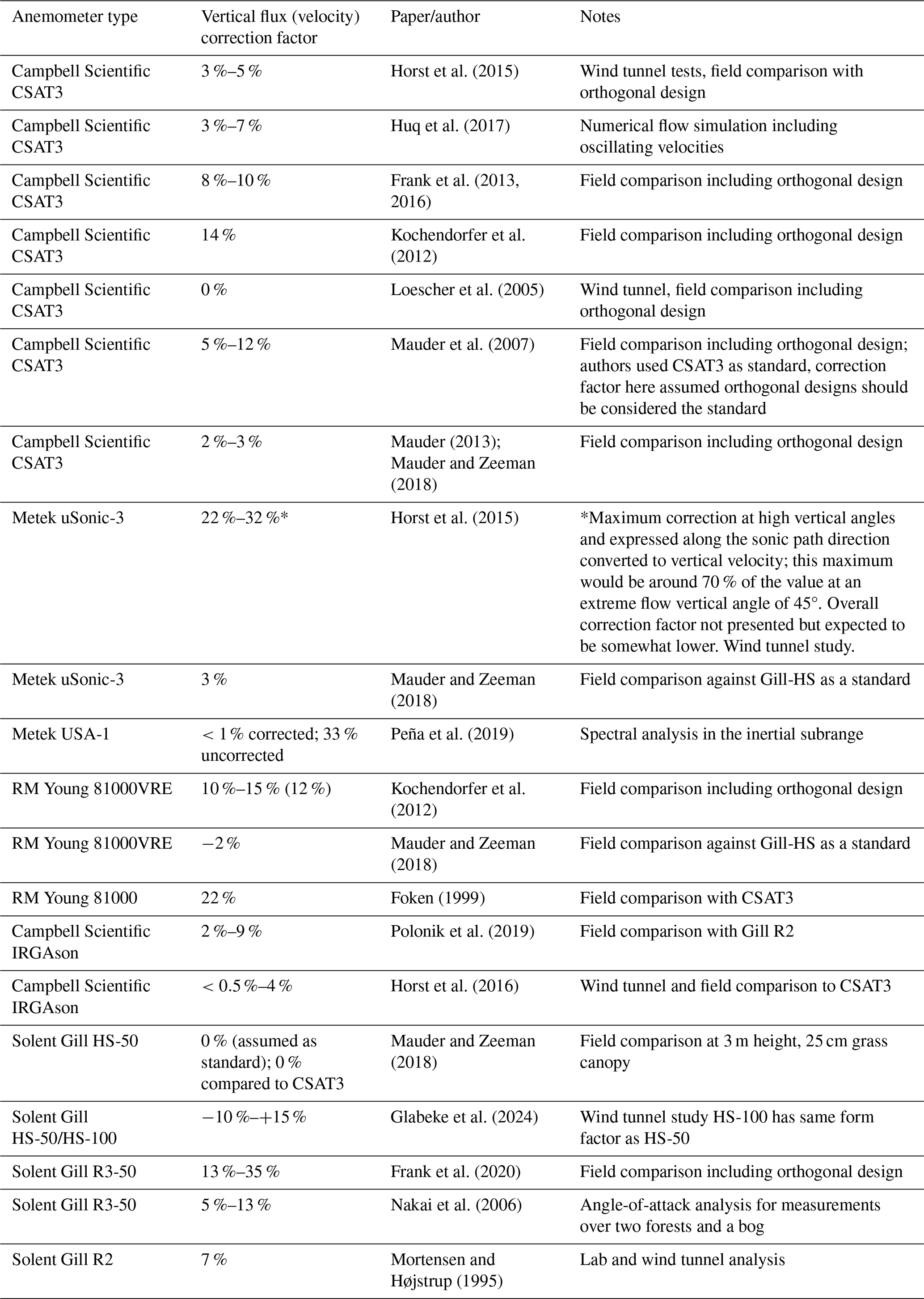
Studies about potential correction factors have involved (1) comparing non-orthogonal sonic anemometers with orthogonal designs; (2) orienting and comparing sonic anemometers, including at different vertical angles both in the field and in wind tunnels; (3) numerical and analytical fluid dynamic simulations of flow around the anemometer configurations and idealized shapes; or (4) examining the spectral output of the anemometers (Wyngaard, 1981; Mortensen and Højstrup, 1995; Foken et al., 1997; Beyrich et al., 2002; Loescher et al., 2005; Nakai et al., 2006; Mauder et al., 2007, 2013; Mauder and Zeeman, 2018; Kochendorfer et al., 2012; Frank et al., 2013, 2016, 2020; Horst et al., 2015, 2016; Huq et al., 2017; Peña et al., 2019). While many of these studies have noted underreporting of the turbulent vertical velocity fluctuations by more than 10 % for some anemometer types, others have found little correction is needed for the vertical velocity (as shown in Table 1).

Table 1 Summary of some selected previous research on vertical velocity correction factors.

In this paper, we test a method that involves standard turbulence data from any individual sonic anemometer (the standard deviation of the vertical velocity, σ_w, and the friction velocity, u^*). From the ratio ${\mathit{\sigma }}_w/u^{*}$ from any single sonic anemometer under near-neutral conditions, a vertical velocity correction factor can be determined, which can henceforth be applied to vertical flux exchange measurements. Although previous papers have discussed using ${\mathit{\sigma }}_w/u^{*}$ to test correction factors derived independently by other fashions and/or a qualitative assessment of measurement validity (Horst et al., 2015; Lloyd, 2023; Wang et al., 2017), none, that we have found, suggest using that ratio itself can independently determine the correction factor. Multiple sonic anemometers do not have to be used for cross-comparison, and some assumptions or limitations used in computational flow simulations at lower Reynolds numbers and wind tunnel studies that have different turbulence regimes, all not necessarily representing field conditions, are not needed. However, our method, as tested here, is not able to examine the change in correction factors with stability as in Horst et al. (2015), but, if an assumed ${\mathit{\sigma }}_w/u^{*}$ relationship is known independently as a function of stability, the method could be extended to non-neutral conditions. We test our method on four types of non-orthogonal anemometers (CSAT3/CSAT3a, IRGAson, Solent Gill HS-50, and RM Young 81000VRE “long neck”), used in seven independent field campaigns, carried out years apart and in two different continents, and directly compare the results of the correction factors by comparing the vertical flux calculations from CSAT3 and RM Young 81000VRE bare ground field data and from CSAT3a and IRGAson bare ground field data under a wide range of stabilities. We use bare ground or short stubbled surfaces primarily to develop the method under relatively ideal conditions.

2 Methodology

2.1 Theory

Our method is based on previously derived sonic data (generally orthogonal sensor design with a vertical sensor path orientation, except Thurtell et al., (1970), which was a pressure sphere anemometer) showing a near-neutral ratio of ${\mathit{\sigma }}_{wm}/u^{*}$ is constant at around 1.3 or, to three significant figures, 1.25 (Thurtell et al., 1970; Haugen et al., 1971; Wyngaard et al., 1971; Merry and Panofsky, 1976; Panofsky et al., 1977; Panofsky and Dutton, 1984; Sharan et al., 1999). The original Kansas experiment data used Kaijo Denki PAT-311 sonic anemometers (Haugen et al., 1971) with a vertical probe path, orthogonal to the plane of the horizontal axis paths. Given that the vertical velocity could be affected by sensor configuration and flow distortion, we define a factor (C_w) that corrects for the potential underestimation of measured vertical velocity w_m (Eq. 1). We assume that any given sonic anemometer should give this ratio under near-neutral conditions. If a sonic anemometer reports a ratio that is lower than 1.25, we can use C_w such that the corrected ratio is 1.25. We recognize that orthogonal sonic anemometer designs may also exhibit flow distortion in the x and y directions while being less likely to distort flow in the vertical direction. This is discussed briefly below further. We also note that if the true ${\mathit{\sigma }}_w/u^{*}$ value were to be assumed equal to 1.2 or 1.3 instead of 1.25, the correction factors we report would need adjustment to be approximately 8 % lower or 8 % higher, respectively.

Applied to non-orthogonal sonic anemometers, the factor C_w can be multiplied by the measured σ_wm to correct for vertical velocity underestimation (Eq. 1). Below we use the subscript “m” to indicate sonic-anemometer-measured values. On the other hand, for correcting measured u^*, the factor would translate to the square root of C_w because u^* is the square root of $\stackrel{\mathrm{‾}}{u_m{w}_m}$ (or even if $\stackrel{\mathrm{‾}}{v_m{w}_m}$ is used in defining u^*, the same result would occur). As shown in Eqs. (2) and (3), the near-neutral ratio of 1.25 to the measured σ_wm over measured u^* (below assuming negligible $\stackrel{\mathrm{‾}}{v_m{w}_m}$ contribution) reported by a sonic anemometer yields the square root of C_w, allowing one to solve for C_w.

$$\begin{array}{}\text{(1)}& {\displaystyle }w=C_w{w}_m;{\mathit{\sigma }}_w=C_w{\mathit{\sigma }}_{wm}\text{(2)}& {\displaystyle }\stackrel{\mathrm{‾}}{uw}=C_w\stackrel{\mathrm{‾}}{w_{m}u};u^{\ast }=\sqrt{C_w\stackrel{\mathrm{‾}}{u{w}_m}}=\sqrt{C_w}{u}_m^{\ast }\text{(3)}& {\displaystyle \frac{{\mathit{\sigma }}_w}{u^{\ast }}}={\displaystyle \frac{C_w{\mathit{\sigma }}_{wm}}{\sqrt{C_w}{u}_m^{\ast }}}=\sqrt{C_w}{\displaystyle \frac{{\mathit{\sigma }}_{wm}}{u_m^{\ast }}}=\mathrm{1.25}\text{(4)}& {\displaystyle }\sqrt{C_w}={\displaystyle \frac{\mathrm{1.25}}{\frac{{\mathit{\sigma }}_{wm}}{u_m^{\ast }}}}\text{(5)}& {\displaystyle }{C}_w={\left({\displaystyle \frac{\mathrm{1.25}}{\frac{{\mathit{\sigma }}_{wm}}{u_m^{\ast }}}}\right)}^{\mathrm{2}}\end{array}$$

We assume that for non-orthogonal anemometers, the horizontal velocities u and v are not significantly underestimated because the typical sensor and physical structure are generally relatively open in the horizontal plane. However if they are affected by either the physical structure or firmware used to calculate orthogonal components or both, the following correction factors for the longitudinal velocity (C_u) and cross-wind velocity (C_v) could be put into Eq. (2) for the more comprehensive equation of u^*, especially above the surface layer, in the boundary layer where $\stackrel{\mathrm{‾}}{v_m{w}_m}$ may be appreciable:

$$\begin{array}{}\text{(6)}& \begin{array}{rl}{u}^{\ast }& =\sqrt[\mathrm{4}]{C_u^{\mathrm{2}}{C}_w^{\mathrm{2}}(\stackrel{\mathrm{‾}}{u_m{w}_m}{)}^{\mathrm{2}}+C_v^{\mathrm{2}}{C}_w^{\mathrm{2}}(\stackrel{\mathrm{‾}}{v_m{w}_m}{)}^{\mathrm{2}}}\\ & =\sqrt{C_w}\sqrt[\mathrm{4}]{C_u^{\mathrm{2}}(\stackrel{\mathrm{‾}}{u_m{w}_m}{)}^{\mathrm{2}}+C_v^{\mathrm{2}}(\stackrel{\mathrm{‾}}{v_m{w}_m}{)}^{\mathrm{2}}}.\end{array}\end{array}$$

Equation (6), if C_u and C_v both equal 1 under ideal conditions, collapses to Eq. (2) for the u^* correction, where u^* could be based on either the surface layer $\stackrel{\mathrm{‾}}{u_m{w}_m}$ or the basic equation expanded in Eq. (6) for conditions when $\stackrel{\mathrm{‾}}{v_m{w}_m}$ cannot be ignored. It should be noted that some surface layer sonic anemometer rotation protocols include the “roll” rotation where $\stackrel{\mathrm{‾}}{v_m{w}_m}$ is minimized, whereas the first two rotations are more straightforward and are more commonly used for pitch and azimuthal (yaw) axis rotations. The same considerations could be applied to orthogonal sonic anemometers; that is, their horizontal velocity components could be distorted (Frank et al., 2016), as earlier alluded to. This has the implication that Eq. (6) could still be used in this case, but the value of 1.25 in the earlier equations might require modification if the horizontal component distortion effects influenced the friction velocity u^*.

Because we are only considering near-neutral conditions, we do not have to worry about the correction factor iteratively influencing the stability parameter ($z/L$), as $z/L$ will be close to zero anyway. The method can also be used to examine if the correction factor is dependent on azimuthal angle, so long as near-neutral conditions occur at those angles. We note our assumptions might not always be strictly applicable, with the non-orthogonal physical configurations coupled with different firmware versions pushing the limits of our assumptions. Also, we assume that the correction factor would be approximately the same in near-neutral conditions as in non-neutral conditions, which may not be true based on the potential for increased pitch angles in turbulent eddies, changing the shadowing factors of sonic anemometer design.

By plotting ${\mathit{\sigma }}_w/u^{*}$ versus $z/L$, we determined the limits of near-neutrality conditions by observing a zone where ${\mathit{\sigma }}_w/u^{*}$ was approximately constant. In most cases, this was in the $z/L$ range between −0.10 and 0. Our data showed a slight increase in ${\mathit{\sigma }}_w/u^{*}$ as the stability transitioned from near zero to stable conditions with $z/L>\mathrm{0}$, so we limited near-neutral stability conditions to the slightly unstable values of $z/L$. In our datasets, the $\stackrel{\mathrm{‾}}{v_m{w}_m}$ contribution to u^* was generally negligible compared to $\stackrel{\mathrm{‾}}{u_m{w}_m}$ because we were measuring in the surface layer, so Eq. (2) could be used.

2.2 Experimental setup and data used

The field campaigns examined here involved bare ground or short stubble with over 100:1 fetch : height ratios. Sonic anemometer data were rotated into the mean wind (azimuth rotation) and vertically (pitch rotation) and were not subject to planar rotation as described by Paw U et al. (2000). Data from a total of 13 Campbell Scientific Incorporated (CSI CSAT3s) were used, of which 12 were used to yield uncertainty estimates for the correction factor. The CSAT3s were examined in four independent field campaigns, with most of the CSAT3 20 Hz data taken from five CSAT3s at 3.45 m height and five CSAT3s at 6.90 m height and summarized in 30 min periods, from the HATS experiment (Kleissl et al., 2003). Two CSAT3s were used at the University of California Davis Campbell Tract experimental site (38°32.2^′ N, 121°46.7^′ W; 18 m a.s.l.) during two different field campaigns, with one CSAT3 at 0.93 m in 2011 and the other in 2005 at 1.2 m (Kochendorfer and Paw U, 2011) and another CSAT3 in a 2018 UC Davis Delta evapotranspiration project (Paw U et al., 2019) at 1.5 m, with data gathered at 10 Hz and summarized for 30 min periods. One CSAT3 was used in an independent comparison with an RM Young 81000 at the C10 site in Roberts Island of the Delta region of the Sacramento–San Joaquin Valley in a UC Davis Delta project (Paw U et al., 2019).

One CSAT3a was studied in a comparison with an IRGAson in Delta site 113, Courtland, California, USA (38°18^′58.59^′′ N, 121°32^′49.24^′′ W; 4 m a.s.l.). Both sensors were installed at 1.7 m from the soil surface, faced the same direction, and were separated horizontally by a 3.2 m distance. For both sonics, data were gathered at 10 Hz and processed using EddyPro, without the shadow correction option selected (see below for a rationale in the discussion of the results from Horst et al., 2015). Two additional IRGAsons were also studied without another sonic anemometer present for comparison. One IRGAson was installed in Clarksburg, California, USA (38°21^′47.16^′′ N, 121°34^′10.85^′′ W; 3 m a.s.l.), at a height of 1.25 m (Delta site 55), while the other was deployed at Walnut Grove, California, USA (38°15^′5.55^′′ N, 121°35^′3.18^′′ W; 3 m a.s.l.), at a height of 1.8 m (Delta site 34). For the IRGAsons, data were gathered at 10 Hz and processed using EddyPro. For the RM Young 81000VRE anemometers, the UC Davis Delta evapotranspiration project campaign data were used for the sonic anemometers mounted at 1.5 m at two different field sites, Roberts Island and Union Island (Paw U et al., 2019), with data logged at 5 Hz. Note that because the RM Youngs internally sample data at 160 Hz, the 5 Hz logging rate does not result in any frequency-related covariance underestimation but can have a slightly greater statistical uncertainty (Bosveld and Beljaars, 2001; Paw U et al., 2018). For the Solent Gill HS-50 sonic anemometers mounted at 2 m, 10 Hz data were from the LIAISE experiment in Spain. The anemometers were mounted on arms oriented 180° from each other. The Land surface Interactions with the Atmosphere in the Iberian Semi-Arid Environment (LIAISE) field experiment took place in the Lleida region of Catalonia, Spain, in the spring and summer of 2021. Although the purpose of the LIASE experiment was to study the impact of agriculture on the water cycle in irrigated regions, there were extensive surface energy budget, surface layer, and boundary layer measurements. One of the LIAISE sites, Els Plans, was located at a fallowed winter wheat field. There was remaining hay and stubble on the ground, so it was not completely bare soil. A 50 m mast was installed at Els Plans, which included eight Gill HS-50s mounted at 2, 10, 25, and 50 m a.g.l. (Brooke et al., 2024). In this study, we only use the 2 m height to ensure that measurements are in the surface layer. There were two anemometers located at 2 m height, “Sonic A” with an orientation of 338° and “Sonic B” with an orientation of 158°.

Table 2 Summary of field experiments used in this study.

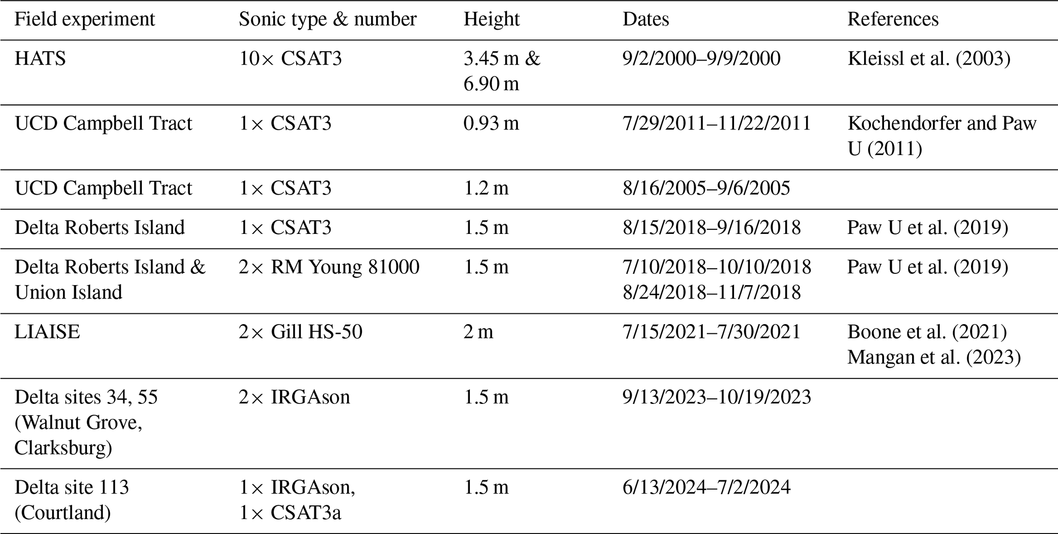
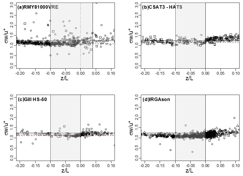
Figure 1 Vertical standard deviation ratio divided by friction velocity (${\mathit{\sigma }}_w/u^{*}$), as a function of stability $z/L$ in the near-neutral interval of −0.20 to 0.10, for four sonic anemometer types. Vertical lines show near-neutral ranges used to determine C_w. A horizontal line indicates the assumed 1.25 ratio. (a) RMY 81000VRE. (b) HATS CSAT3s. (c) Gill HS-50 sonic anemometer. (d) IRGAson sonic anemometers. Circles are for site 113, squares for site 55, and triangles for site 34. Dashed lines indicate the median ratio (${\mathit{\sigma }}_w/u^{*}$) determined in the near-neutral range; for the Gill HS-50, the long black dashed lines indicate the median ratio for “Sonic B”, and the shorter red dashed lines indicate the median ratio for “Sonic A”.

${\mathit{\sigma }}_w/u^{*}$ data were filtered for wind directions coming into the anemometer in a default range of $+/-\mathrm{45}$° centered towards the maximum fetch and sonic anemometer orientation, in the opposite direction from the tower/mast mounts, to minimize the influence of any flow distortion not caused by the transducers and their mounts. Different ranges of azimuthal angles were examined. For the 10 HATS CSAT3s that had two heights, 3.45 and 6.90 m, with 5 individual CSAT3s at each height, data were only used when approximately constant flux conditions existed, that is, when the u^* between the two heights were within 5 % of each other. Near-neutral was defined as unstable conditions with zeta $>-\mathrm{0.1}$ and <0.00 for most cases, except for the RM Young 81000VRE case where the near-neutral zeta was defined for zeta $>-\mathrm{0.1}$ and zeta <0.04 (see Fig. 1). Zeta is defined here as $z/L$, where z is the height of measurement, and L is the Monin–Obukhov length.

At the UC Davis Delta Roberts Island C10 site, both an RM Young 81000 and a CSAT3 were run at the same time, so an application test of our theory was made by correcting both the CSAT3 and the RM Young 81000 sensible heat H data with their respective C_w correction factors to see if the corrected data from the two separate sonic anemometers would agree better than if they were uncorrected. At Delta site 113, a test of the theory was made by comparing a CSAT3a with an IRGAson, to see if the theoretical correction factors matched the sensible heat H data for these two sonic types.

3 Results and discussion

3.1 Correction factors C_w

This method yields vertical velocity and vertical flux C_w correction factors compatible with previous studies using other methods, especially for the CSAT3s. Of the four sonic anemometer types analyzed, the IRGAson (see further discussion below) and RM Young “long neck” anemometers had the greatest C_w correction factors of 1.19–1.37; the Solent Gill HS-50s had a correction factor of 1.21 (average of 1.283 and 1.137); and the CSAT3s and the CSAT3a had correction factors of 1.11–1.23 (median 1.13), with a standard deviation of 0.07 for the 13 CSAT3 anemometers.

Table 3 Vertical velocity correction factors C_w calculated in this study.

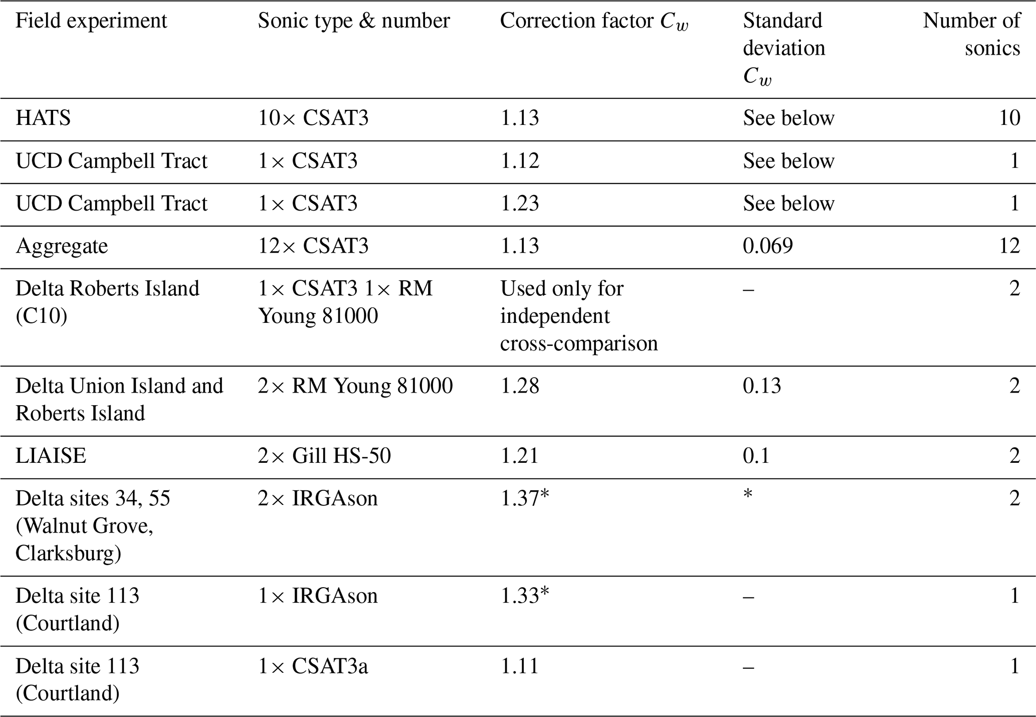
^* Cross-comparison with CSAT3a indicates assumptions made to calculate the theoretical C_w are not fully applicable for the IRGAson form factor. The IRGAson practical correction factor C_w should be the same as the CSAT3a, as explained in the text.

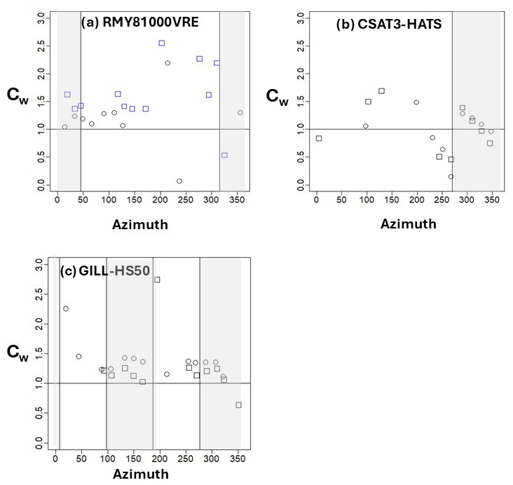
Figure 2 Correction factor C_w for the RM Young 81000VREs as a function of azimuthal angle relative to north (a), the HATS CSAT3s (b), and the Gill HS-50s (c). The vertical lines and gray shading represent the optimum angles between 315 and 45° as assessed during the experimental design phase (a), between 270 and 360° (b), and between 97–187° for the circles and 277–7° for the square symbols (c). For the RM Young 81000s, the circles represent data from the Roberts Island site, and the squares Union Island. For the CSAT3s, the circles represent the median for five sonic anemometers at the 3.45 m height and the squares five sonic anemometers at the 6.90 m height. For the Gill HS-50, the circles represent a sonic on the arm oriented to the east, and the squares the sonic on an arm oriented to the west, with block medians taken for the correction factors spanning 20° intervals.

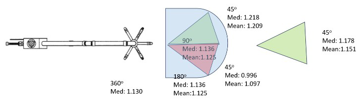
Figure 3 Correction factor C_w as a function of azimuthal angle sectors, for the HATS CSAT3 data.

The proposed method was tested for the correction factor C_w as a function of azimuthal angle ranges for the Gill HS-50s (Fig. 2). The proposed method was also tested for correction factor C_w as a function of azimuthal angle ranges for the CSAT3s (Figs. 2 and 3). Because the IRGAson geometry is asymmetrical when viewed in the x-axis direction of the sensor, we examined correction factors for different azimuthal angles. However, the details of the IRGAson are not presented here, as we present evidence that our theoretical method's assumptions appear not to have been met when analyzing the IRGAson.

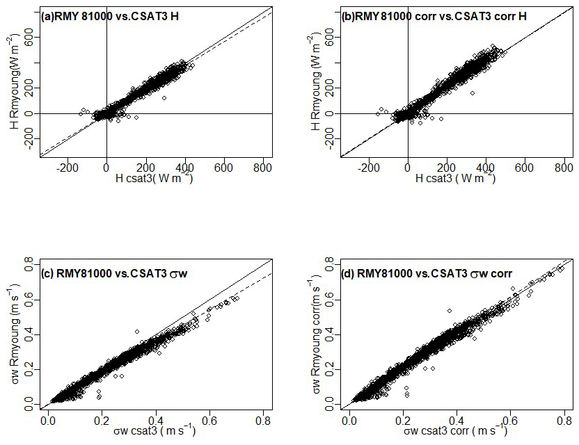
Figure 4 (a) Uncorrected RM Young 81000VRE sensible heat plotted against uncorrected CSAT3 sensible heat, with the regression line $Y=\mathrm{0.9465}X-\mathrm{0.4533}$ W m⁻² shown by a dashed line and the 1:1 line shown by a solid line. (b) Corrected RM Young 81000VRE sensible heat plotted against corrected CSAT3 sensible heat, with the regression line $Y=\mathrm{0.9947}X-\mathrm{0.5383}$ W m⁻² shown by a dashed line. (c) Uncorrected RM Young 81000VRE σ_w plotted against uncorrected CSAT3 σ_w, with the regression line $Y=\mathrm{0.90354}X+\mathrm{0.0005112}$ m s⁻¹ shown by a dashed line. (d) Corrected RM Young 81000VRE σ_w plotted against corrected CSAT3 σ_w, with the regression line $Y=\mathrm{1.0235}X+\mathrm{0.0006543}$ m s⁻¹ shown by a dashed line.

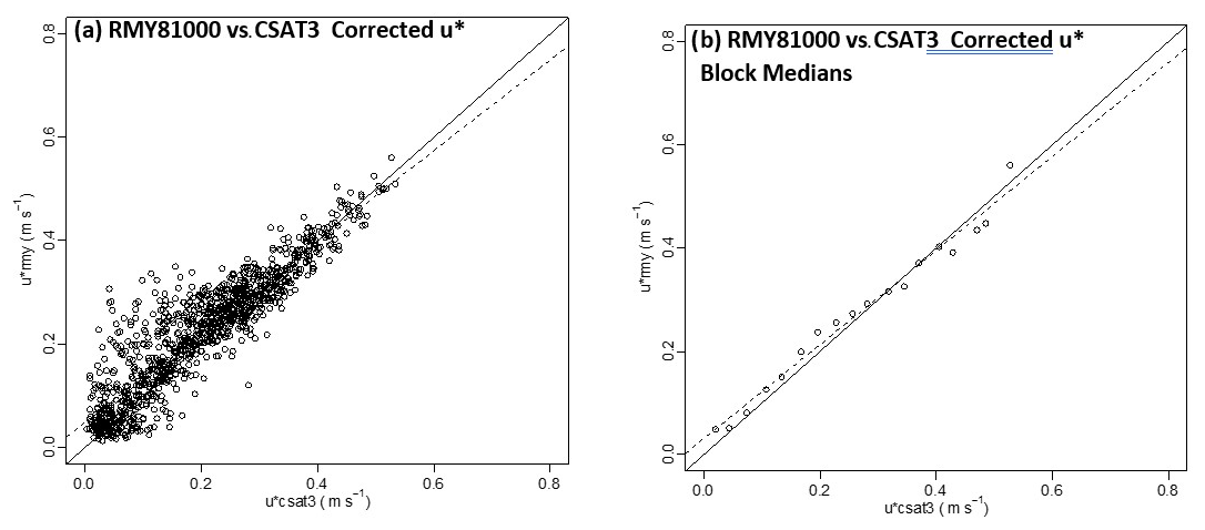
Figure 5 (a) Corrected RM Young u^* plotted against corrected CSAT3 u^*, $Y=\mathrm{0.9384}X-\mathrm{0.03225}$ m s⁻¹. (b) Block medians of corrected RM Young 81000 u^* plotted against corrected CSAT3 u^*, $Y=\mathrm{0.9345}X+\mathrm{0.0302}$ m s⁻¹.

3.2 Sonic anemometer field intercomparisons

The correction factors were tested on the CSAT3 and RM Young 81000 sited in the Delta fallow field for the sensible heat. When the CSAT3 was corrected with the average CSAT3 factor of 1.13, and the RM Young 81000 corrected by its individual correction factor using our method (1.188), there was excellent agreement (Fig. 4, slope of 0.9947, intercept of −0.538 W m⁻²), but when the RM Young 81000 was corrected by the average factor from Table 4 (1.28), the sensible heat of the RM Young 81000 was overcompensated (slope of 1.07, intercept of −0.58 W m⁻²) (not shown in figures). The uncorrected sensible heat showed the RM Young 81000 H was lower than that for the CSAT3 (slope of 0.947, intercept of −0.453 W m⁻², Fig. 4). The excellent agreement implies that the correction method is applicable for a range of stabilities and not confined to near-neutral conditions for vertical scalar fluxes and for these two sensor head configurations but that some uncertainty in correction can occur when using the average correction factors. The uncorrected vertical velocity standard deviation shows the RM Young 81000 was lower than the CSAT3 (slope of 0.9035,intercept of 0.000511 m s⁻¹), while the corrected data had a slope of 1.0235 and an intercept of 0.000654 m s⁻¹ (Fig. 4). The agreement for u^*, on the other hand, was not as good, although it still improved the agreement, with a corrected (for the individual RM Young 81000) slope of 0.9384 and intercept of 0.032 m s⁻¹ (Fig. 5), compared to the uncorrected slope of 0.8817 with an intercept of 0.0285 m s⁻¹. The figure shows a great deal of overestimated scatter for the RM Young u^* in the intermediate range of u^* from around 0.05 m s⁻¹ to around 0.2 m s⁻¹; taking block medians of the data over intervals of the x axis to reduce the effect of the scatter did not change the regression results much, with a similar slope of 0.9345 and intercept at 0.030 m s⁻¹ (Fig. 5). This implies some of the assumptions we have made may be violated in terms of the distortion or firmware influences on the horizontal velocity measurements and the correlation coefficient between the vertical and horizontal velocity components, when applied to a range of stabilities. This issue affects the u^* calculation more than the simpler vertical velocity correction for the scalar sensible heat flux.

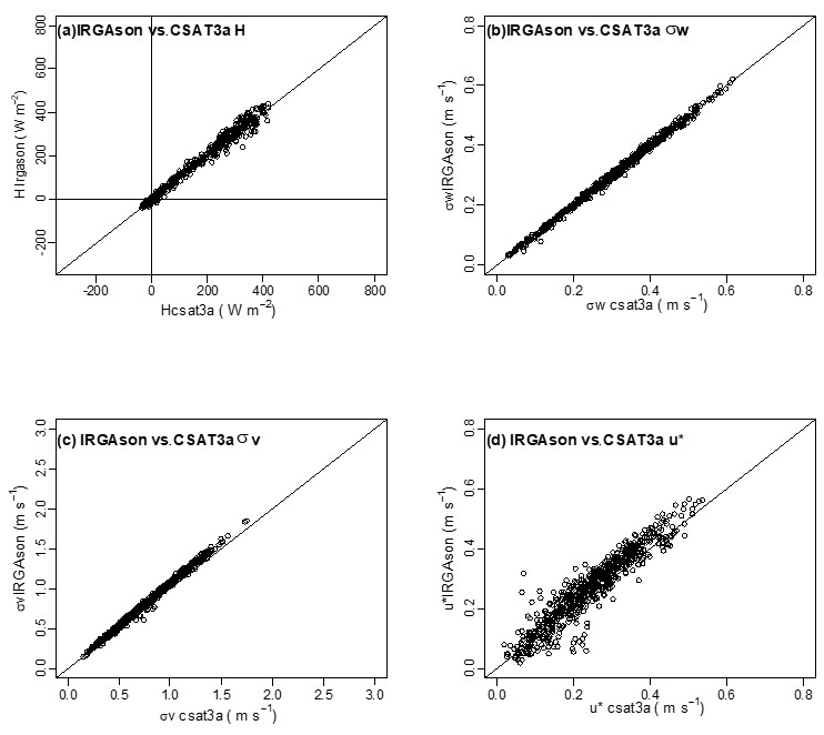
Figure 6 Comparison of (a) Sensible Heat, H, (b) vertical velocity standard deviation, σ_w, (c) cross wind velocity standard deviation σ_v and (d) u^* between the CSAT3a and IRGAson at Delta site 113.

In the field test between the CSAT3a and the IRGAson, sensible heat covariance $\stackrel{\mathrm{‾}}{w^{\prime }{T}^{\prime }}$ was within 1 %, and the σ_w was also within 1 % (Fig. 6). This implies the vertical velocity correction factor for the IRGAson should be considered the same as for the CSAT3a, that is a C_w of around 1.11, similar to that for CSAT3s. However, our ${\mathit{\sigma }}_w/u^{*}$ analysis method results in a C_w of 1.33–1.37 for the IRGAson (Table 3), which contrasts with the direct comparison between the two anemometers. Analysis of the data shows the IRGAson u^* was greater than that for the CSAT3a, including at near-neutral conditions, creating a greater value for C_w from our method (Fig. 6). This was not seen in the standard deviations of the longitudinal and vertical wind components but did show up in the cross-wind standard deviation (matching earlier reports of the cross-wind anomalies in Horst et al., 2016), so this implies that either the complex sensor head geometry, the internal data processing, or both yielded this overestimate of Reynolds stress covariance and u^* while not relatively affecting the vertical velocity measurements compared to the CSAT3a (Fig. 6). Horst et al. (2016) reported that the IRGAson yielded a lower u^* than their reference CSAT3s, but they calculated their u^* as the surface layer stress based on $\stackrel{\mathrm{‾}}{u^{\prime }{w}^{\prime }}$, while we were using the total Reynolds stress term with both $\stackrel{\mathrm{‾}}{u^{\prime }{w}^{\prime }}$ and $\stackrel{\mathrm{‾}}{v^{\prime }{w}^{\prime }}$, which could explain our different results for u^*. The basic assumptions in our theory that only the vertical velocity would be affected and that the effect would propagate into u^* as a square root relationship compared to a direct propagation into the vertical velocity were apparently not appropriate for the IRGAson. This result also means that the departure of the IRGAson's ratio ${\mathit{\sigma }}_w/u^{*}$ from the idealized 1.25 value cannot be used as a general quality control assessment for its vertical eddy covariance measurements, a method suggested in some sources (Horst et al., 2016; Wang et al., 2017; Lloyd, 2023).

Literature data for the ratio of ${\mathit{\sigma }}_w/u^{*}$ in near-neutral conditions also were generally compatible with our analysis. While the CSAT3/CSAT3a C_w correction factors (1.11–1.23, median 1.12) are close to literature CSAT3 values (1.03–1.14), the literature IRGAson factors of 1.005–1.09 are somewhat lower than our theory's calculation of 1.33–1.37 but similar to the correction factor of 1.11 for the IRGAson when based on the theoretical correction factor for the CSAT3a and the observed equivalence of the sensible heat and vertical velocities between these two sonic head configurations at a common test site. Horst et al. (2015) reported a ${\mathit{\sigma }}_{wm}/u^{*}$ value of 1.17 for uncorrected CSAT3 data, which using our method would yield a C_w of 1.14, well within our range of CSAT3 C_w results. They also reported a similar ${\mathit{\sigma }}_{wm}/u^{*}$ value (1.16) for the shadow correction that can be implemented in models like the CSAT3a or IRGAson, so it appears that implementing the built-in shadow correction option would not affect our method or results. Interestingly, the method applied to instruments over tall canopies yields comparable values to the literature and our study but with some difference. Wang et al. (2017) report, for a 10 m forest canopy and sonic anemometers 5 m above this height, the near-neutral ${\mathit{\sigma }}_{wm}/u^{*}$ values of 1.19 and 1.18 for IRGAson and Gill WindMaster, which would translate to C_w correction factors of 1.10 and 1.12, respectively, using our method. The RM Young 81000 comparison by Foken (1999) of a 22 % correction relative to a CSAT3 would translate to an absolute correction of 38 %, or higher than our value of 28 %, if the CSAT3 is considered to have a 13 % correction. The Gill HS-50 results of 21 % correction is higher than the range of literature values. The lowest literature value was assumed to be 0 % (Mauder et al., 2017) and approximately equal to the CSAT3 when compared with other sonic anemometers (Horst et al., 2016), which would then imply a 13 % correction between −10 % and +15 % (Glabeke et al., 2024).

4 Summary and conclusions

We present a method to estimate vertical velocity and flux corrections for sonic anemometers, using commonly reported turbulent statistics from a single anemometer, instead of comparisons that require the test anemometer and reference orthogonal sonic anemometers to be side by side, laboratory or numerical methods, or methods requiring raw high frequency data. The vertical velocity factor C_w is multiplied by vertical eddy covariance fluxes to correct them for transducer shadowing. This method could provide correction factors associated with objects near the test anemometer, such as the tower or mast mounting assembly, electronic support environmental enclosures, and solar panels, in addition to transducer and sonic anemometer head design flow distortion to the vertical wind speed.

Application of our correction method could improve energy budget closure by 10 % to over 20 % depending on the anemometer type and would thereby increase calculated eddy-covariance-based fluxes. Several assumptions are made which may not always be applicable, and here we present tests over relatively ideal sites with low roughness (bare ground or stubble and good fetch). Our study demonstrates that the standard deviation of the vertical velocity and friction velocity data gathered under near-neutral stability from an individual sonic anemometer can be used to estimate a vertical velocity and vertical flux correction factor, for some of the most common sonic anemometers, under any stability conditions. The values are consistent with the literature for the CSAT3 range of suggested correction factors (1.13), the CSAT3a at 1.11, and the Gill HS-50 (1.21), while the correction factor for the RM Young 81000VRE is higher, 1.28. The theoretical correction factor of 1.33–1.37 for the IRGAson did not match results from a direct comparison with a CSAT3a, and our direct field comparison implied the CSAT3a correction factor of 1.11 should also be used for IRGAsons. This implies our theory's assumptions did not appear valid for the IRGAson configuration, partially because of cross-wind turbulence overestimation, probably related to the relatively complex IRGAson form factor. Our results also mean that one general quality assessment of eddy covariance vertical fluxes, based on the closeness of the near-neutral values of ${\mathit{\sigma }}_w/u^{*}$ to 1.25, cannot be reliably applied to the IRGAson or other similar sonic anemometer systems with unusual shape/form factors but is appropriate for usage with typical sonic anemometers like the CSAT3 family, RM Young 81000VRE, the Gill HS-50, and similar anemometers. This form of analysis could be tested in the future for usage over taller roughness landscapes, such as crops, orchards, and forests, given enough fetch for measurement heights over the roughness layer.