Algorithm for continual monitoring of fog based on geostationary satellite imagery

This study presents an algorithm for the detection of fog and low stratus (FLS) over Europe based on the infrared bands of the SEVIRI (Spinning Enhanced Visible and InfraRed Imager) instrument on board the Meteosat Second Generation geostationary satellites. As the method operates based on the SEVIRI infrared observations only, it is expected to be stationary in time and thus can provide a coherent and detailed view of FLS development over large areas over the 24 h day cycle. The algorithm is based on a gradient boosted tree machine learning model that is trained with ground truth observations from METeorological Aerodrome Report (METAR) stations and the SEVIRI observations at bands centered at 8.7, 10.8, 12.0, and 13.4 µm wavelengths. The METAR data used here comprise a total number of 2 544 400 data points spread over the winters (i.e., 1 September to 31 May) of the years 2016–2022 and 356 locations across Europe. Among them, the data points corresponding to 276 stations and the winters of 2016–2018 and 2019–2021 (∼ 45 % of all data points) were used to train the algorithm. The remaining data points comprise four independent datasets which were used to validate the algorithm's performance and applicability to time spans and locations within the study area (i.e., Europe) that extend beyond those covered by the data points used for the algorithm training, as well as to compare the algorithm's accuracy at the locations of METAR stations with that of the existing state-of-the-art daytime FLS detection algorithm Satellite-based Operational Fog Observation Scheme (SOFOS). Validation of the algorithm against the METAR data showed that the algorithm is well suited for the detection of FLS. Specifically, the algorithm is found to detect FLS with probability of detection (POD) values ranging from 0.70 to 0.82 (for different inter-comparison approaches) and false alarm ratios (FARs) between 0.21 and 0.31. These numbers are very close to those achieved by SOFOS for differentiating FLS from other sky conditions at the tested locations and time spans. These results also showed that the technique's applicability in the study region extends beyond the particular locations and time spans covered by the data points used for training the algorithm.

1 Introduction

Fog and low stratus (FLS) are both persistent aggregations of water particles in liquid and/or solid phases, i.e., clouds close to the Earth's surface. As the cloud base height is the only real difference between the two (fog: touching the ground; low stratus: above ground), they are frequently treated together as a single category from the satellite perspective (i.e., FLS). FLS influences various aspects of life on the Earth: on the one hand it may act as source of water supply (e.g., Shanyengana et al., 2002; Lehnert et al., 2018), as well as a modifier in the global climate system (Vautard et al., 2009). On the other hand, it causes large economic costs in the transport, health, and energy sectors (Köhler et al., 2017; Pérez-Díaz et al., 2017). For these reasons, continuous (and ideally near-real-time) detection of FLS and monitoring of its spatiotemporal patterns and developments is essential. An important application lies in solar energy usage. With the rising share of electricity generated from photovoltaic (PV) systems, the prediction of current and future solar irradiance and, hence, PV power output becomes crucial for the operation of modern power grids. In the context of PV power production, the detection and monitoring of FLS is particularly important as FLS, unlike moving clouds, can persist longer and impact larger regions simultaneously, making regional power grid balancing a challenging task.

Geostationary satellites have an outstanding potential for the detection and monitoring of FLS. That is because they continuously scan the Earth from the same angle over the 24 h of the diurnal cycle, providing spatiotemporally coherent spectral images of the Earth. To exploit this potential, to this day several FLS detection methods have been developed and applied (e.g., Ellrod, 1995; Cermak and Bendix, 2008, 2007; Egli et al., 2018; Nilo et al., 2018; Kim et al., 2019; Underwood et al., 2004; NWC SAF, 2019; Fuchs et al., 2022; Klüser et al., 2015), which detect FLS by performing a sequence of spectral and/or spatial tests on satellite measurements. Although these methods have proven to be useful exploring the FLS characteristics (e.g., Cermak et al., 2009; Egli et al., 2017; Pauli et al., 2022a, b, 2024), they usually consist of a solar-zenith-angle-dependent and separate daytime and nighttime schemes, making use of spectral channel characteristics particular for either night or day. This, however, makes the continuous monitoring and forecasting of FLS life cycle and occurrence at the critical point of the day (i.e., sunrise) impossible. For example, an FLS detection method may operate based on shortwave reflectances, as FLS-covered regions typically have high reflectivity and smooth texture in the visible spectral region (Lee et al., 2011). But as no reflectance data are available during nighttime, a whole other algorithm would be required to be applied over nighttime. FLS can also be detected by testing the difference between the brightness temperatures in medium-wave (MIR) and long-wave (LIR) infrared bands (typically referring to radiation at wavelengths between 3–8 and 8–15 µm, respectively) against threshold values. That is because the FLS droplets are typically smaller than those of other cloud types. As a result, FLS shows a greater contrast between the brightness temperatures measured at MIR and LIR bands compared to other clouds (Hunt, 1973). However, as MIR has a solar component during daytime, application of this technique requires daytime and nighttime separation. This is, for example, the case for the cloud-type product (includes FLS) which can be derived from the algorithm APOLLO-NG (AVHRR Processing scheme Over cLouds, Land and Ocean – Next Generation; Klüser et al., 2015) and the software package NWC/GEO (NWC SAF, 2019), which is also used by the Royal Netherlands Meteorological Institute for producing the MSG-CPP products (available at https://msgcpp.knmi.nl/, last access: 17 February 2025). To overcome this limitation and enable consistent FLS detection across the entire diurnal cycle, an approach that relies solely on observations in the LIR bands would be required.

The main objective of the present study is to develop and validate a single fully diurnal FLS detection algorithm for Europe based on geostationary satellite observations. The guiding hypothesis of the present study is that FLS can be discriminated from cloud-free regions and non-FLS clouds based on spectral LIR data with an accuracy comparable with the existing state-of-the-art daytime FLS detection algorithms. Satellite detection of FLS using only LIR bands only is a quite challenging task and historically believed to be a rather impossible one (Güls and Bendix, 1996). That is mainly because FLS emits at temperatures very close to that of the Earth's surface. Nonetheless, Andersen and Cermak (2018) succeeded at developing a method for FLS detection over the Namib desert (located in southern Africa) which operates solely based on the brightness temperatures measured at the LIR bands of the Spinning Enhanced Visible and InfraRed Imager (SEVIRI) sensor on board the Meteosat Second Generation (MSG) spacecraft. Specifically, they discriminated FLS from cloud-free land by analyzing the spatial structure (texture) of images constructed from the differences between the brightness temperatures measured at 12.0 and 8.7 µm SEVIRI channels. The main underlying assumptions associated with this method are (i) the 12.0–8.7 µm values are typically greater for clouds than for land surface, and (ii) the 12.0–8.7 µm calculated for bare soil shows a higher level of spatial heterogeneity compared to smooth FLS top surfaces. Andersen and Cermak (2018) showed that, although small, there are distinct differences between the spectral signatures of a clear land and FLS in the LIR region, which makes their distinction possible. Nevertheless, this method is applicable to regions where the mentioned assumptions are met (i.e., deserts and possibly arid regions) and cannot be easily extrapolated to the much more complex geospheric and atmospheric conditions of Europe. Therefore, to this date, no approach for the continual 24 h detection of FLS over Europe exists.

This study presents and validates a single machine learning (ML) algorithm for the detection of FLS over land across Europe, based on Meteosat–SEVIRI bands centered at 8.7, 10.8, 12.0, and 13.4 µm wavelengths. Furthermore, it provides an intercomparison between the accuracy of this method and that of the existing state-of-the-art daytime FLS detection algorithm Satellite-based Operational Fog Observation Scheme (SOFOS; Cermak and Bendix, 2008; Cermak, 2006) to address the objectives of the study. The method presented here is based on a gradient boosted tree (XGBoost) ML model that is trained with observations from METeorological Aerodrome Report (METAR) stations and the LIR observations of SEVIRI on board Meteosat-10 and Meteosat-11 platforms. As the method presented here operates solely based on the spectral data in the LIR region, it is expected to be applicable during the 24 h of the diurnal cycle over European lands. Thus, it is suitable for continuous monitoring of FLS over Europe and can reveal a detailed view of the diurnal and spatial patterns of FLS over Europe. This can be of essential value for the analysis of FLS occurrence and related processes as well as improvement of methods for PV power forecasting. It can also serve as a precondition for statistics-based nowcasting.

2 Data

2.1 Satellite observations

SEVIRI is a multi-purpose scanning (passive) radiometer on board MSG geostationary satellites operated by the European Organization for Exploitation of Meteorological Satellites (EUMETSAT; Aminou, 2002). This instrument has been in operation by EUMETSAT at 0° latitude and longitude at the altitude of ∼ 35 800 km above mean sea level since early 2004 and is intended to remain in service at 0° until 2033 (expected lifetime of the last MSG mission, i.e., Meteosat-10). SEVIRI measures upwelling radiance at the top of the atmosphere (TOA) for the Earth's whole disk covering Europe, the North Atlantic, and Africa in 12 spectral channels in 15 min intervals (12 min scanning time followed by 3 min of processing time). Eleven of the SEVIRI channels are narrow-band channels which are spread over the spectral region between 0.56 (visible) to 14.4 µm (LIR) and have a sampling spatial resolution of 3×3 km² at nadir. The remaining one is a broadband high-resolution visible channel (0.6–0.9 µm) with a sampling resolution of 1 km at nadir. The level 1.5 product of SEVIRI (Hanson and Mueller, 2004; Schmetz et al., 2002; Tranquilli et al., 2016) consists of geolocated, radiometrically preprocessed TOA upwelling radiances observed by SEVIRI (spacecraft-specific effects have been removed) at its 12 channels. The present study uses the level 1.5 radiances measured by MSG SEVIRI instruments positioned at 0° latitude and longitude. The data include measurements from channels centered at 0.6, 0.8, 1.6, 3.9, 8.7, 10.8, and 12.0 µm wavelengths. These data were acquired from EUMETSAT (EUMETSAT, 2017) for the region covering Europe and north Africa and includes the winter periods (i.e., 1 September–31 May) between the years 2016 and 2022. These data were measured by the SEVIRI instruments on board the MSG-3 and MSG-4 platforms. The acquired data were calibrated and converted to reflectances (ρ; for 0.6, 0.8, and 1.6 µm channels) and brightness temperatures (BTs; for 3.9, 8.7, 10.8, 12.0, and 13.4 µm channels) following the procedure explained in EUMETSAT (2017) using the satpy Python package (Martin et al., 2021). The summer months (i.e., June, July, and August) were excluded from the analysis because the FLS occurrence frequency is very low over these months (Egli et al., 2017) and their inclusion in the analysis largely affects the imbalance between the observed FLS-positive and FLS-negative cases (see Table 1 for more information).

2.2 SOFOS

As a reference for the newly developed algorithm, the existing and validated satellite-based Operational Fog Observation Scheme (SOFOS; Cermak and Bendix, 2008; Cermak, 2006) was used. A daytime-only technique, this approach was developed specifically for MSG SEVIRI and makes use of the visible, mid-infrared, and thermal-infrared channels in a series of threshold tests. These include per-pixel spectral tests as well as tests applied on spatially coherent and distinct areas of pixels.

2.3 Ground-based observations

The METAR (METeorological Aerodrome Report) data comprise the reports of weather measurements performed at a network of meteorological stations located at airports across the world. The primary objective of these measurements is aviation safety, but they also have an application in meteorology. The METAR parameters cloud base height (CBH; m), sky cloud cover (CC; okta), and horizontal visibility (HV; km) for the period 1 September 2016 to 31 May 2022 were acquired and used in the present study to identify the FLS conditions based on ground-based observations. These parameters are either retrieved automatically (instrumentation is not standardized) or estimated by human observers at each station at temporal frequencies of 1 h or less. The temporal frequency of the observations performed at these stations is related to the weather conditions, airport size, and traffic. In particular, stations located at large and busy airports are equipped with automatic devices and tend to have a higher frequency of observations compared to small airports. Also, under weather conditions violating flight safety such as fog occurrence or extreme weather, the frequency of the observations at these stations is increased to ensure flight safety.

The acquired data were first subjected to a quality control procedure to filter out the stations with unreliable observations. Specifically, the stations not meeting at least one of the following conditions were considered unreliable and were discarded from the analysis: (1) average number of observations per hour greater than 1.5 for the data period, (2) average number of empty observations less than 0.05 during the data period, or (3) continuous data gaps less than 1 month. The underlying assumption for defining these tests is that the data from stations with a rather homogeneous frequency of observations is more likely to have reliable accuracy and consistency. The quality control thresholds applied here have been defined empirically and as such are restrictive enough to filter out the stations with unreliable observations and yet relaxed enough to get a reasonable number of temporally homogeneous observations for further analysis. By applying the abovementioned filters, 591 out of 947 stations were discarded. The locations of the remaining 356 stations were spatially matched with the SEVIRI grid using the smallest distance between the center of each SEVIRI pixel and the station location. For the temporal matching, the METAR times of observation were first rounded up to the closest 15 min intervals (t_m) of SEVIRI. Then, the SEVIRI images with the timestamps t_m+15 min were considered the temporally matched images, as the actual SEVIRI scanning time for the study area is much closer to the end of each 15 min interval. The location of these stations is illustrated in Fig. 1. As can be inferred from this figure, the stations selected are spread across Europe (plus four in north Africa), covering a wide range of regions with various surface types, altitudes, and meteorological conditions.

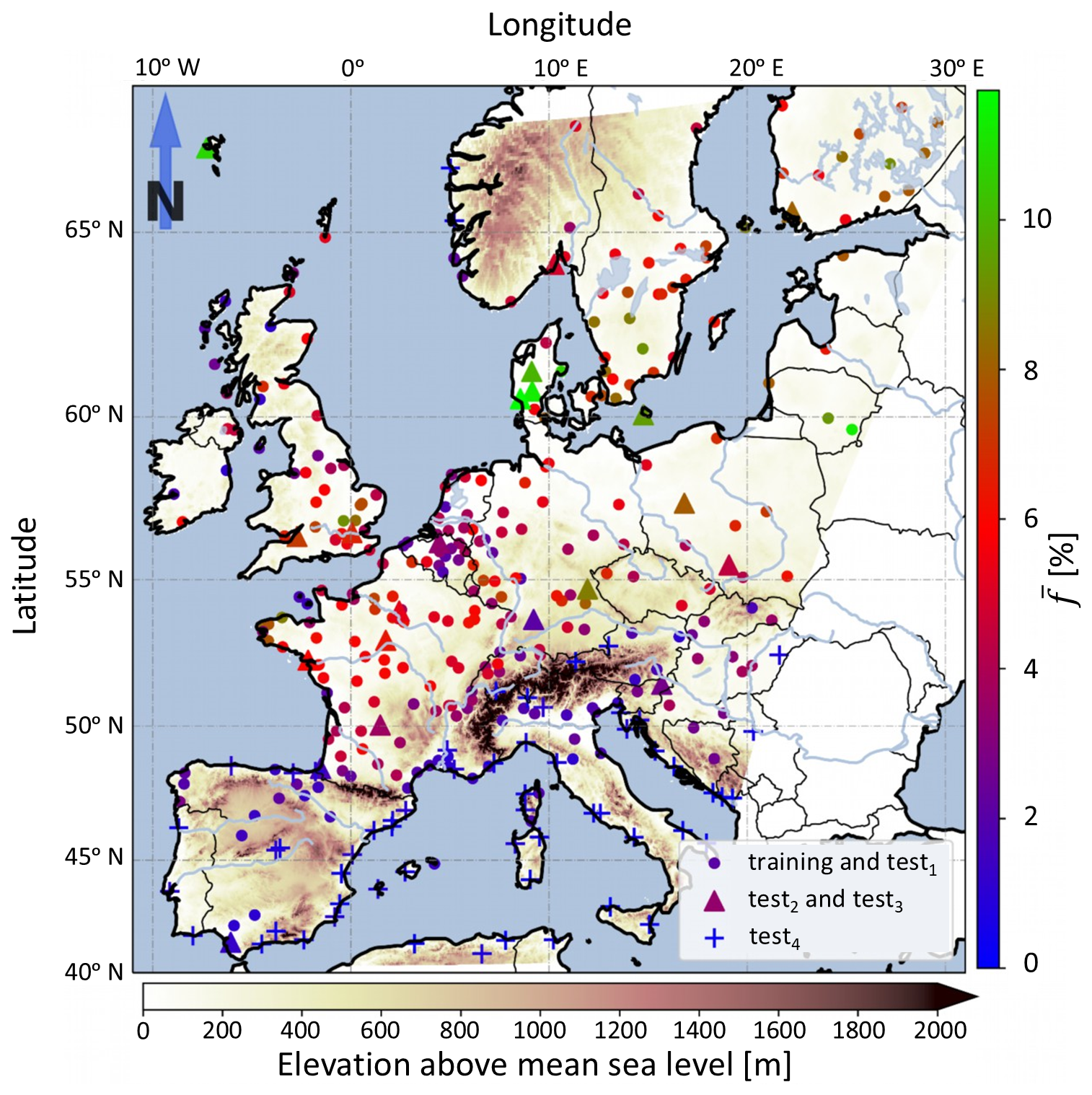
Figure 1 Geographical location of the selected ground observation (METAR) sites. The horizontal color bar indicates the elevation above mean sea level for the study area (m; obtained from EUMETSAT Satellite Application Facility on Land Surface Analysis: last access: 16 January 2023 – 13:36 GMT+1). The filled circles show the geographical locations of the stations included in the training and test₁ datasets. The triangles illustrate the geographical locations of the stations included in the datasets test₂ and test₃ (see Sect. 2.4 for more information). The locations of the stations included in the test₄ dataset are shown with plus (“+”) signs. The vertical color bar indicates the mean annual FLS occurrence frequency ($\stackrel{\mathrm{‾}}{f}$; %) at the location of the station as described in Sect. 2.4 of the paper based on the modified ground-based FLS labels (before selecting the confident labels).

3 Methods

3.1 FLS labels

The present study uses the ground-based identified FLS occurrences as the basis for algorithm development and validation purposes. The FLS occurrences were identified using the CBH, CC, and HV measurements performed at the selected METAR stations (see Sect. 2.2 for more information). Fog was defined by HV values below 1 km and low stratus by CBH below 1 km and CC above 5 oktas (Egli et al., 2017). Then, Observations with either fog or low stratus were marked FLS-positive, while those missing HV, CBH, or CC data were marked undefined. Observations with neither fog nor low stratus were labeled FLS-negative.

The FLS labels produced this way indicate whether FLS is detected from the perspective of a ground-based observer/instrument. However, these labels may not be consistent with what is observed from space, as the satellite's field of view (FOV) may be contaminated with layers of non-FLS clouds passing through its line of sight (LOS). This is particularly relevant in Europe, where about 30 % of FLS events are obscured by other clouds (Cermak, 2018). Additionally, the FLS-negative labels indicated above do not specify the sky condition (cloudy or cloud-free land) in the satellite's FOV. To cope with these two issues, the non-FLS clouds blocking the satellite's LOS were identified using the SEVIRI spectral measurements. Particularly, a series of spectral tests were performed using the collocated SEVIRI ρ_0.6, ρ_1.6, BT_3.9, BT_8.7, BT_10.8, BT_12.0, and BT_13.4 data corresponding to each data point. These tests are the same as those used in the SOFOS algorithm for classification of the SOFOS classes “water”, “cirrus”, and “ice” clouds (Cermak and Bendix, 2008) and can discriminate non-FLS clouds from FLS and cloud-free land.

The ground-based FLS labels were updated based on the above-mentioned tests performed on the SEVIRI data as follows: FLS-negative observations from ground data were classified as “clear-sky” if no non-FLS clouds were detected and as “non-FLS-cloud” if clouds were present. For FLS-positive points, those with non-FLS clouds present were classified as “multi-layer” (FLS beneath non-FLS clouds), while others remained “FLS”. It is worth mentioning that as the non-FLS cloud screening procedure explained above uses the SEVIRI ρ_0.6, and ρ_1.6 data, its applicability is limited to daytime (i.e., solar zenith angles ≤80°). For this reason, despite the availability of both the SEVIRI and METAR data over day and night, the FLS labels derived here are limited to the daytime only. It should also be noted that, despite overall reliability of the procedure applied here for the detection of non-FLS cloud contaminated cases, the method sometimes fails to detect non-FLS clouds, leading to occasional misclassifications (e.g., multi-layer or non-FLS-cloud cases labeled as FLS or clear-sky). Nevertheless, initial tests of a machine learning model showed that using this procedure is essential for making the ground observations compatible with what is seen from space.

3.2 FLS flag quality assessment

The quality of the modified FLS labels in terms of sky condition homogeneity was assessed by comparing the labels corresponding to each timestamp at each station with that of its previous and next timestamps at the same station. Particularly, for each three consecutive data points at the same location the middle data point was set to

• “no confidence” if the time difference between the first and third data points was greater than 1 h or the FLS label if neither the first nor the third data point were the same as the middle one;

• “semi-confident” if the FLS label for one of the first or third data points was the same as that of the middle one;

• “confident” if the FLS label for both the first and third data points was the same as that of the middle one.

This quality control procedure was considered to identify data points with a homogeneous sky condition and to minimize the uncertainties associated with spatiotemporal matching of the SEVIRI data with the ground station data, the coordinate system used for geolocation of SEVIRI pixels, and coordinates of the ground stations. The SEVIRI pixels have a spatial resolution of about 3 km at nadir which results in a resolution between 4 and 8 km over Europe. Plus, there is up to 0.3 km of uncertainty associated with the procedure applied by EUMETSAT for georeferencing SEVIRI images. Additionally, the satellite is not exactly stationary on the geostationary ring, and its true position varies slightly with time because all satellites are drifting from their nominal position. On the other hand, the ground stations are not exactly located at the center of the SEVIRI pixels, and some are indeed on the borders of the pixels. Also, there may exist occasions where the METAR location within the pixel has a different sky cover compared to the majority of the pixel area. This can be the case with pixels contaminated by the edges of non-FLS clouds or cloud layers which are forming but are not yet fully developed (see Jahani et al., 2020, 2022; Koren et al., 2007). The sky conditions for the data points surviving this quality control procedure are assumed to be homogeneous at the subpixel level.

3.3 Training and testing datasets

The entire data were split into five datasets, namely “training”, “test₁”, “test₂”, “test₃”, and “test₄”. Table 1 summarizes the characteristics of these datasets, and Fig. 1 shows the location of the stations included in each of them. The training dataset was used for training the ML algorithm. The test₁ dataset was intended to evaluate the performance of the trained model over locations seen by the model during training but at time spans beyond those used for model training. The datasets test₂, test₃, and test₄ were intended for quantifying the accuracy of the trained model over locations which were never seen by the model during the whole study period. The sampling for the data split was done based on the time frame of the observations and the FLS occurrence regimes identified according to FLS flags described in Sect. 2.4.

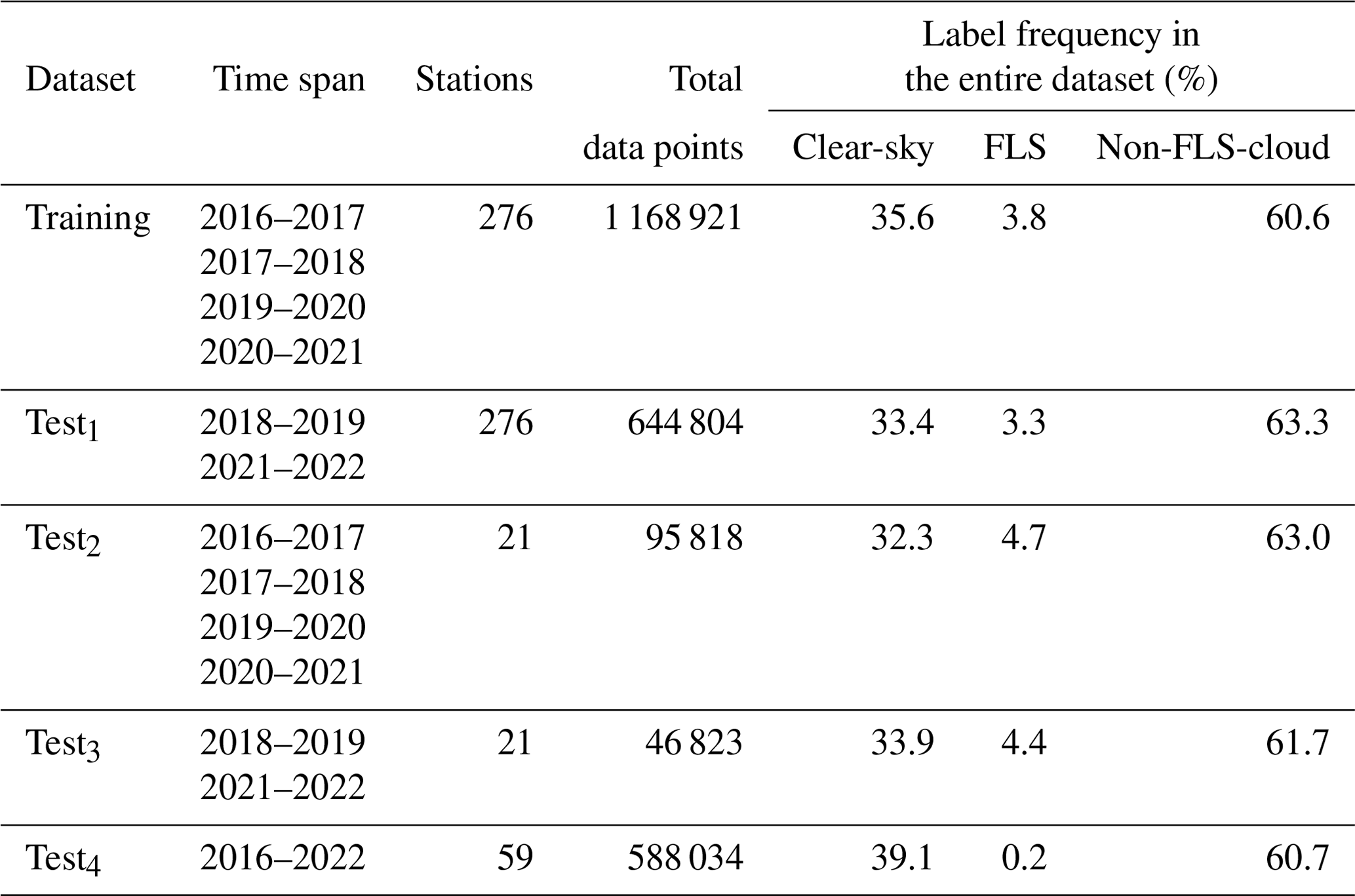
To split the data, the annual frequency of FLS occurrence at each station was first determined by calculating the ratio of the daytime FLS-positive labels to all valid labels in METAR per winter year (i.e., 2016–2017, 2017–2018). In the second step, the annual ratios were averaged over the study period to obtain the mean annual frequency of FLS occurrence at each station ($\stackrel{\mathrm{‾}}{f}$, range of the values obtained: 0.0 %–12.0 %). In the third step, the stations were grouped into 23 bins based on their $\stackrel{\mathrm{‾}}{f}$ values (bin widths: 0.5 %). The entire data corresponding to the stations falling in the first two $\stackrel{\mathrm{‾}}{f}$ bins (i.e., $\stackrel{\mathrm{‾}}{f}<\mathrm{1}$ %) were considered the test₄ dataset (59 stations). This dataset was intended to evaluate the algorithm's performance at locations where FLS rarely occurs. In the fourth step, from each of the 21 remaining $\stackrel{\mathrm{‾}}{f}$ bins, one random station per bin was selected to construct the test₂ and test₃ datasets. Among all the data points corresponding to these 21 stations, those that cover the winters (September to May) of 2018–2019 and 2021–2022 comprise the test₃ dataset, and the remaining ones comprise the test₂ dataset. These two datasets are considered for validating the algorithms at locations other than those used for training the ML model. As can be understood, the difference between the two is the time span covered by them. In particular, the time spans covered by the test₂ dataset are the same as those of the dataset used for training, and test₃ dataset covers time spans beyond those covered by the training dataset. Lastly, the test₁ and training datasets were then constructed by splitting the data corresponding to the 276 stations which were not allocated to test₂, test₃ or test₄. Specifically, the data points corresponding to the winters (September to May) of 2018–2019 and 2021–2022 comprised the test₁ dataset, and those corresponding to the winters of 2016–2017, 2017–2018, 2019–2020, and 2020–2021 comprised the training dataset. As can be inferred, the data points corresponding to the stations with $\stackrel{\mathrm{‾}}{f}$ less than 1 % were not included in the training dataset. These data were excluded from the training dataset to decrease the imbalance between the FLS-positive and FLS-negative cases. That is because the initial tests of the algorithm indicated that the data corresponding to the stations with $\stackrel{\mathrm{‾}}{f}$ less than 1 % in the training dataset vastly increase the imbalance between FLS-positive and FLS-negative cases, which leads to a decrease in the algorithm's skill for detecting the FLS cases. These data points were, however, included in the analysis as the test₄ dataset to evaluate the algorithm's performance at places that FLS rarely occurs. Next, the cases of “no confidence” and “semi-confident” FLS were removed from the five datasets, and the cases of “multi-layer” conditions were relabeled as non-FLS-cloud for the test₁, test₂, test₃, and test₄ datasets but were removed completely from the training dataset. They were removed from the training dataset to eliminate cases that could introduce ambiguity, ensuring the ML model is trained on data with a clear distinction between non-FLS-cloud and the two other classes (i.e., clear-sky and FLS). The METAR FLS labels generated in this way (hereafter referred to as “MFLs”) serve as the ground truth and will be used for the model development and validation purposes. A summary of the data included in the final four datasets is given in Table 1. A schematic description of the process followed in this section for the creation of the MFLs included in all five datasets is provided in Fig. A1. As this table shows, the training, test₁, test₂, and test₃ datasets contained an overall number of 1 168 921, 644 804, 142 641, and 588 034 data points, respectively. This table also shows that the number of non-FLS cases (i.e., clear-sky and non-FLS-cloud classes combined) is substantially higher than the FLS cases. Nevertheless, the fraction of FLS cases is in the same range for the datasets training (3.8 %), test₁ (3.3 %), test₂ (4.7 %), and test₃ (4.4 %), whereas that of test₄ (0.2 %) is considerably lower than that of the other three datasets. It should be noted that the FLS labels prior to the application of quality flags were used for the data split because the goal was to sample data based on different FLS regimes, whereas the quality checks were mainly applied to flag data points that are likely to represent homogeneous sky conditions.

Table 1 Summary of the data contained in the training, test₁, test₂, and test₃ datasets. The values given in this table are based on the final datasets (i.e., they are derived based on confident FLS labels).

3.4 Machine learning algorithm

In the present study, an XGBoost (gradient boosted tree) model was developed for FLS detection over Europe based on SEVIRI observations in the LIR (long-wave infrared) spectral region. XGBoost is a well-tested supervised ML (machine learning) technique which has been successfully applied to many regression and classification problems. It extracts the nonlinear relationships between sets of input variables/features and a target output variable through constructing an ensemble of sequentially built regression trees (also referred to as “weak learners”) to the data. The regression trees are added one at a time to the ensemble to correct for the deficiencies in the previous regression tree and to minimize a specified loss function. All these trees together construct a powerful statistical model referred to as “XGBoost”. For this model, the prediction is performed by summing over all the regression trees. Once the model is trained, the role of each input feature in constructing the boosted decision trees within the model is indicated based on a metric referred to as “feature importance”. The more an input feature is used to make key decisions with decision trees, the higher its importance. For more information about XGBoost, refer to Mitchell and Frank (2017), Friedman (2001), and Natekin and Knoll (2013). The open-source XGBoost Python implementation (https://xgboost.readthedocs.io/en/stable/index.html, last access: 28 March 2023) was used in the present study.

The XGBoost model was trained to predict the labels FLS, non-FLS-cloud, and cloud-free based on a set of input variables generated from the channel combinations BT_12.0, BT_8.7–BT_12.0, BT_10.8–BT_12.0, and BT_12.0–BT_13.4 plus the standard deviation of each of these variables in a spatial window 3×3 pixels in size with the central pixel being the target pixel.

The pixel values of the mentioned variables contain information about the cloud presence, cloud top height, phase, and the particle radius for the area falling within the limits of the target pixel. Specifically, the SEVIRI channels centered at 8.7, 10.8, and 12.0 µm wavelengths fall within the atmospheric window region (where the absorption by the atmospheric gases is minimal) and the one at 13.4 µm is in a CO₂ absorption region. BT_8.7–BT_12.0 and BT_10.8–BT_12.0 provide data on the spectral dependency of the emissivity of the surface/cloud covering the scanned scene. These data give information about the size and thermodynamic phase of the particles at the cloud top (Strabala et al., 1994) in the case of cloudy scenes and about surface properties for the clear-sky scenes (e.g., Petitcolin and Vermote, 2002; Andersen and Cermak, 2018). BT_12.0–BT_13.4 is linked to the absorption depth of CO₂, which can be used as a proxy for determining the depth of the atmospheric column. This information can be interpreted as the height of the emitting body (surface/cloud). BT_12.0 is a proxy for the temperature of the emitting body, which can play a role in the determination of its height and phase. The standard deviations of the channel combinations mentioned above summarize the heterogeneity of this information over the 3×3 pixel area around the target pixel. The standard deviations were considered because the different land and cloud types tend to show different degrees of spectral and spatial heterogeneity.

The hyperparameters of the model were tuned to optimize the model's performance and avoid overfitting. This was done based on the statistical indicators explained in Appendix B. To this aim, a grid search was performed to find the optimum values of the XGBoost hyperparameters learning rate (0.3), maximum depth (5), minimum child weight (1), number of regression trees (100), alpha (0), and lambda (1). The XGBoost model trained this way was then applied to all SEVIRI scenes acquired in the present study (see Sect. 2.1), including the SEVIRI pixels over water.

3.5 Feature selection

The set of input variables mentioned in Sect. 3.4 was selected by analyzing the spectral SEVIRI LIR data and the corresponding MFLs included in the training dataset with the objective of creating the simplest model possible that can capture general differences between FLS and the two other classes (i.e., non-FLS-cloud and cloud-free). Here, the simplest model is defined as an accurate model (according to Eqs. B1–B7) capable of detecting FLS based on minimal spectral and spatial input data. To select the most relevant input features for discriminating FLS from the two other classes (i.e., those that reduce the error the most), we tested the data corresponding to the LIR channels centered at 8.7, 9.7, 10.8, 12.0, and 13.4 µm wavelengths along with all the 10 possible combinations which can be derived from subtracting them from one another. This was done by applying the feature selection technique referred to as “backwards elimination”. To this aim, an XGBoost model was initially trained to predict FLS labels using all the input features. The features were then iteratively removed (one feature was dropped per iteration) based on their low gains in fitting (feature importance), leading to a series of models totaling 15. The simplest combination of input features was then selected by comparing the accuracy of models 2 to 15 with that of the first model (the most complex one was considered the reference). This revealed that the accuracy drops gradually as features decrease, with a significant drop when a key feature is removed. The model just before this drop signifies the minimal essential feature set. Additional tests also indicated that including the standard deviations of these variables in a 3×3 pixel area around the target pixel helps to increase the accuracy of the model, and for this reason they were considered input features to the model.

3.6 Validation

The skills of the newly proposed ML and the existing SOFOS FLS detection algorithms were quantified and compared by validating them against the MFLs corresponding to the training, test₁, and test₂ datasets. The validation for each dataset was performed by calculating the statistical indicators probability of detection (POD), false alarm ratio (FAR), probability of false detection (PFD), critical success index (CSI), accuracy (ACC), bias score (BS), and distance from optimal point (d) as indicated in Appendix B. These statistical indicators were calculated using all data points included in each dataset to evaluate and compare both algorithms' overall performance over the training and four test datasets.

4 Results and discussion

Figure 2 summarizes the results obtained from validating the ML and SOFOS FLS algorithms against the MFLs corresponding to the training, test₁, test₂, test₃, and test₄ datasets. The statistical indicators given in this figure were calculated using all data points present in the five datasets (see Table 1 for more information); therefore they can be interpreted as the overall performance of the algorithms over all regions and time spans covered by each dataset. Validation of the ML product versus the MFLs included in the training dataset revealed an overall classification accuracy of 0.60 and 0.98 in terms of CSI and ACC metrics for the algorithm, respectively. The algorithm was able to correctly label about 80 % of the FLS and 99 % of the non-FLS (clear-sky or non-FLS-cloud) situations included in the training dataset (POD: 0.80; PFD: 0.99). The FAR score obtained by the ML product for the same dataset was 0.30, which resulted in a d of 0.36. The FAR of 0.30 indicates that 30 % of the situations labeled as FLS by the ML product were reported as non-FLS by the ground-based MFLs. Because of these false alarms the FLS occurrence frequency computed for the training dataset based on the ML product is overestimated by about 14 % compared to the determination made by the MFLs (BS: 1.14). Overall, these numbers show that the ML algorithm proposed here was capable of detecting the majority of the FLS situations over the locations and time spans included in the training dataset. Considering that the algorithm was trained using these exact data points, it can be inferred that the algorithm was able to capture the subtle yet discernible distinctions between FLS and non-FLS situations (in the LIR spectral region) at locations and time spans covered by the training dataset. This is further reinforced by comparing these error metrics with those calculated for the daytime SOFOS algorithm for validation versus the same dataset: the CSI, ACC, and PFD scores obtained by SOFOS were 0.59, 0.98, and 0.98, respectively, which are close to what was obtained by the ML algorithm. On the other hand, SOFOS showed a higher POD (0.92) compared to the ML algorithm, which was achieved at the cost of a higher FAR (0.38), leading to larger d and BS (0.38 and 1.47, respectively). Specifically, the number of data points labeled as FLS by SOFOS was 14 027 (29 %) greater than what was reported as FLS by the ML algorithm. Only about one-third of these data points, however, were correct calls, and the rest were false alarms. In fact, all of these false alarms must have been identified as clear-sky by the MFLs. That is because the criteria considered in the MFLs for screening out the non-FLS clouds is the same as the one used by SOFOS. Thus, the case of the non-FLS-cloud class included in the MFLs matches well with that of SOFOS, and the validation approach presented here essentially evaluates the skill of SOFOS in discriminating the FLS and clear-sky situations from each other. One implication of these differences can be the fact that the ML algorithm considers a stricter criterion compared to SOFOS for classifying a situation as FLS, resulting in a more confident FLS identification. On the other hand, these misclassifications could also correspond to the cases of snow-covered land under clear-sky conditions. Nonetheless, heterogeneity of topography at a subpixel scale could have a strong impact on this evaluation. This is particularly important here due to the coarse resolution of the SEVIRI pixels over Europe. Subpixel heterogeneity of topography can be problematic for validating these products as the sky conditions in the area covered by the SEVIRI pixel are not well represented by station measurements. Specifically, there may exist situations where the station measurements indicate a clear-sky condition, whereas the majority of the SEVIRI pixel area is covered by FLS (and vice versa). However, understanding the influence of topographical heterogeneity at a subpixel scale on the FAR and BS scores can be quite challenging and is out of the scope of the current study.

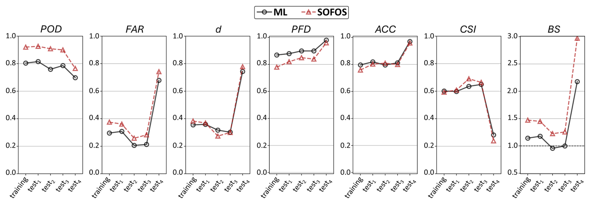
Figure 2 Validation results of the ML (black circles) and SOFOS FLS detection algorithms (red triangles) versus the modified METAR FLS labels (MFLs) for the training, test₁, test₂, test₃, and test₄ datasets.

Based on the preceding discussion, it can be inferred that the ML algorithm is competent and appropriate for distinguishing between FLS and non-FLS situations. This accomplishment aligns with the initial hypothesis of this study, which states that spectral LIR data can be used to differentiate FLS from cloud-free land and non-FLS clouds with comparable accuracy to an existing state-of-the-art daytime FLS detection algorithm. The information provided in Fig. 2 overall suggests that the ML algorithm applicability expands beyond locations and time periods covered by the training dataset. Specifically, the results obtained from validation versus the test₁ dataset confirm the technique's applicability to time periods that are not included in the training dataset. The CSI, ACC, and PFD scores obtained by the ML model for validation versus the test₁ dataset were, respectively, equal to 0.60, 0.98, and 0.99, which are the same as those reported for the training dataset. Nonetheless, POD and FAR values derived from validating the ML algorithm with the test₁ dataset were slightly higher than those obtained through validation with the training dataset (0.82 and 0.31, respectively). Consequently, this results in a slightly increased BS (1.18), while the value of d remains the same (0.36). As can be inferred from Fig. 2, the statistics obtained by the ML algorithm over test₂ and test₃ compare very well with those obtained by SOFOS. In particular, ACC, CSI, and PFD were merely the same for both algorithms over the two test datasets. On the other hand, the POD and FAR values obtained by SOFOS were both higher than those obtained by the ML algorithm, which results in a similar d but higher BS scores. Validation with the test₂ dataset confirms the algorithm's FLS detection capability at locations outside the training dataset but within the same time spans. The results obtained from the test₃ dataset prove the algorithm's effectiveness at locations and time periods not encountered during training. Validation versus the test₄ dataset is particularly important here because neither of the two algorithms were originally designed for regions included in the dataset. Nonetheless, results obtained from this validation should be interpreted with care due to the low number of FLS cases (as identified by MFLs) included in this dataset. In particular, the test₄ dataset only includes nearly 0.2 % FLS cases, and as a result, even one random misclassification can have a strong impact on the error metrics FAR, d, CSI, and BS. For this reason, the evaluation of the algorithm in this region is done solely based on the metrics POD, PFD, and ACC. As can be seen in Fig. 2, validation of the ML (SOFOS) algorithm with test₄ yielded high values of POD, PFD, and ACC equal to 0.70 (0.76), ∼ 1.0 (∼ 1.0), and ∼ 1.0 (∼ 1.0), respectively. These numbers prove that the ML algorithm developed in the present study is applicable to regions where FLS rarely occurs.

Overall, the error metrics given above (and shown in Fig. 2) show that the ML FLS detection algorithm developed here is suited for application over Europe. In particular, the algorithm features an accuracy very similar to that of the state-of-the-art daytime SOFOS algorithm but has the advantage of operating based on SEVIRI LIR bands, which allows its application over the 24 h of the diurnal cycle. It is worth mentioning that the error metrics calculated here for SOFOS are somewhat different compared with those reported in Cermak and Bendix (2008) and Egli et al. (2018) for this algorithm, although the METAR data were used for validation purposes in the two studies. Specifically, the POD, FAR, and CSI, as reported by Cermak and Bendix (2008) for SOFOS, ranged from 0.76 to 0.83, 0.02 to 0.06, and 0.73 to 0.82, respectively. In the study by Egli et al. (2018), the reported values of POD and FAR for SOFOS were 0.52 and 0.66, respectively. There are several reasons contributing to these differences. One reason can be the additional processing steps involved in the present study for the generation of MFLs compared to the other two studies: applying the quality flags and marking the non-FLS cloud contaminated pixels. The difference in the location of the stations selected and the number of data points utilized for the validation highly impact the validation results. Additionally, as these error metrics are calculated as relative statistics, the absolute number of FLS and non-FLS cases included in the datasets used for validation can make a big difference in the results obtained. This is particularly important here because they are calculated relative to a small subset of the data: the FLS-positive cases (as identified by the truth or predicted product) which are inherently low in number. This is especially relevant in Europe, where about 30 % of FLS events are obscured by other clouds (Cermak, 2018). As a result of the relatively small denominator, they can show a relatively high degree of sensitivity to a few misclassifications. In addition, it should be noted that they do not provide a global image about the overall classification accuracy of the product, as they do not account for the true-negative instances, which are very large in number for FLS. For these reasons, although the metrics POD, FAR, CSI, and BS provide essential and detailed information about the product's performance, they need to be interpreted with care. To account for these two matters the error metrics ACC and PFD were introduced. As the denominator of these metrics is rather large and they take the true-negative instances into consideration, they are expected to be better suited for showing the product's overall performance over the whole dataset.

Figure 3 provides detailed insights into the false-negative and false-positive (see Appendix B) predictions of the FLS ML technique across the five datasets. In Fig. 3a it can be seen that the majority (∼ 80 %–90 %) of pixels falsely classified as FLS by the ML algorithm (i.e., false alarms) were actually clear-sky pixels. Similarly, Fig. 3b shows that ∼ 83 %–92 % of false-negative pixels (i.e., undetected FLS pixels) were predicted as clear-sky pixels by the ML algorithm. These results suggest that the algorithm has room for improvement in distinguishing between clear sky and FLS. Indeed, finding it challenging for the algorithm to separate clear-sky from FLS (especially in the complex geo- and atmospheric conditions of Europe) is expected because FLS emits at temperatures close to the Earth's surface, resulting in only small differences between the LIR spectral signatures of clear-sky and FLS conditions. Although the algorithm shows some limitations in distinguishing between clear-sky and FLS, its performance is acceptable for meeting the objectives of the study, especially given that it is a lightweight approach relying solely on calibrated MSG SEVIRI LIR data. Nevertheless, its accuracy can be further enhanced by incorporating auxiliary datasets. For example, integrating digital elevation maps (e.g., as in Egli et al., 2018) and surface or atmospheric temperature and humidity information from external sources (e.g., from reanalysis as in NWC SAF, 2019) could improve POD and FAR. Additionally, applying pixel- or spatial-based pre- and/or postprocessing steps, such as those used in Pauli et al. (2022a) and Andersen and Cermak (2018) may help to better identify FLS events and correct potential misclassifications, leading to a decreased FAR. These enhancements, however, fall outside the scope of the present study and are left for future work.

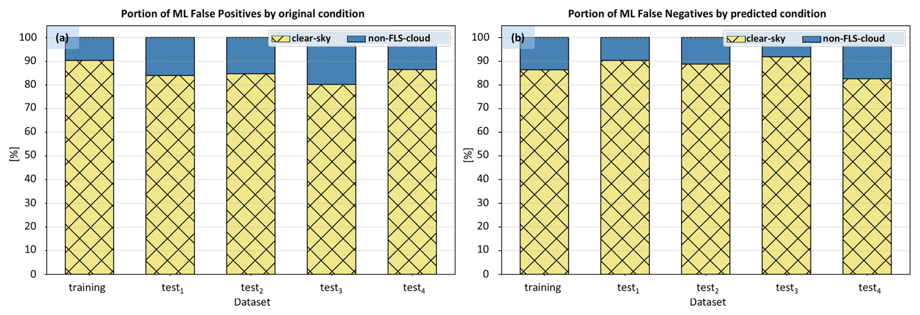
Figure 3 Detailed information on false-positive and false-negative (see Appendix B) predictions of the FLS ML technique across training, test₁, test₂, test₃, and test₄ datasets. Panel (a) shows the percentage of false-positive instances that were clear-sky and non-FLS cloud contaminated according to the ground truth dataset (i.e., MFL). Panel (b) shows the percentage of false-negative instances that were categorized as clear-sky and non-FLS-cloud by the ML algorithm.

Figure 4 illustrates the calibrated SEVIRI level 1.5 products over the study region on 2 March 2021 – a representative day with the presence of persistent FLS in Europe – at three distinct scan times (13:00, 16:30, and 20:00 UTC), along with the corresponding outputs generated by the ML FLS detection algorithm developed in this study. In this figure, the panels in the left column (a, d, and g) show ρ_0.6. Panels in the middle column (b, e, and h) show a false-color RGB image constructed based on the SEVIRI LIR data, with the red, green, and blue channels being BT_12.0–BT_13.4, BT_8.7–BT_12.0, and BT_10.8–BT_12.0, respectively. Panels in the right column (c, f, and i) illustrate the classifications produced by the ML FLS detection algorithm, with the classification categories including clear-sky (khaki), FLS (red), and non-FLS-cloud (blue). In each panel, solar zenith angle values are represented by colored contour lines. The data presented in this figure highlight the consistency of the ML FLS detection algorithm across different conditions: daytime (top row), the day–night transition (middle row), and nighttime (bottom row), as well as over various surface types, including water, land, and land–water transition points. Supplement Video S1 shows the full sequence of the false-color RGB satellite images and the corresponding classification maps over the 24 h cycle of 2 March 2021.

The presence of a widespread FLS event around 55° N, with partial contamination by non-FLS clouds can be observed in Fig. 4a. Additionally, two smaller regions are visible: one near 50° N, 15° E and another near 50° N, 10° W. These areas are characterized by a smooth texture and high reflectivity. In Fig. 4b, the FLS-covered regions are distinguishable by their smooth texture and dark red coloration, while the non-FLS clouds appear in green with greater spatial variability compared to FLS regions. Figure 4c demonstrates the algorithm's effectiveness in identifying both FLS-covered regions and the non-FLS clouds passing over these areas. Notably, the algorithm's performance remains robust, with no sudden changes or misclassifications observed, even when applied to water, land, or land–water transition points. Apart from slight changes in the coverage, FLS persists over the mentioned regions until the end of that day (see Supplement Video S1 for more information), which can be traced in Fig. 4e and h. As can be seen in Fig. 3f and i, the algorithm continues to accordingly and consistently identify the FLS-covered regions over land and water during the day–night transition time and at night. Here again, the algorithm's performance remains robust, with no sudden or solar-zenith-angle-dependent changes/misclassifications observed.

However, it is worth mentioning that for the three scans shown here the algorithm categorizes the area near 47° N, 10° E (the Alps), which appears to be snow-covered, as non-FLS cloud contaminated. This is because, as Fig. 4b, e, and h show, snow-covered land and non-FLS clouds exhibit similar characteristics in the LIR range.

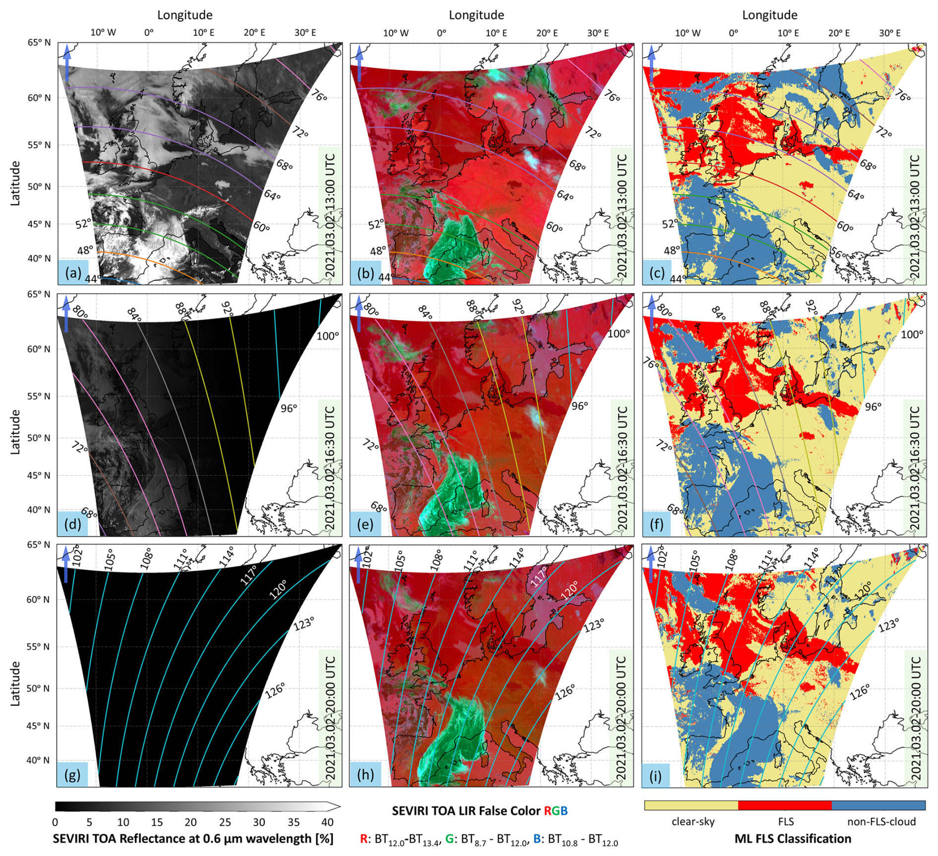
Figure 4 Comparison between calibrated SEVIRI level 1.5 products over the study region on 2 March 2021 at three different scan times (13:00, 16:30, and 20:00 UTC) and the corresponding outputs yielded from the ML FLS detection algorithm developed in the present study. Panels in the left (a, d, and g), middle (b, e, and h), and right columns (c, f, and i), respectively, represent ρ_0.6 (%); false-color RGB composite based on BT_8.7, BT_12.0, and BT_13.4; and the classifications produced by the ML FLS detection algorithm. FLS classification categories include clear-sky (khaki), FLS (red), and non-FLS-cloud (blue). Overlaid colored contour lines represent solar zenith angle (degrees) for reference. Note: solar zenith angles greater than 95° are represented in turquoise. Supplement Video S1 shows the full sequence of the false-color RGB satellite images and the corresponding classification maps over the 24 h cycle of 2 March 2021.

5 Summary, conclusions, and outlook

The main objective of the present study was to develop a diurnally stable algorithm for the detection of FLS over Europe based on observations from the SEVIRI instrument on board MSG satellites with an accuracy comparable with that of a state-of-the-art daytime FLS detection algorithm. The algorithm proposed here consists of a gradient boosting (XGBoost) machine learning model that is trained to classify each SEVIRI pixel as clear-sky, FLS, or non-FLS-cloud based on SEVIRI observations in the LIR bands. Specifically, the classification is performed based on pixel values of BT_12.0, BT_8.7–BT_12.0, BT_10.8–BT_12.0, and BT_12.0–BT_13.4 plus the standard deviation of each of these variables in a spatial window 3×3 pixels in size with the central pixel being the target pixel.

A total of 6 years of daytime ground-based observations from METeorological Aerodrome Report (METAR) stations at 356 European locations were utilized to generate ground truth FLS labels for training and evaluating the algorithm. Lastly, a comparison between the accuracies of the newly proposed ML and the existing daytime FLS detection algorithm (SOFOS) was performed to address the objective of the study.

The results obtained from validating the FLS products against the training and the four test datasets revealed that the ML FLS detection algorithm proposed here is capable of discriminating FLS from other sky conditions and that its applicability in the study region (i.e., Europe) extends beyond the particular locations and time spans covered by the data points used for training the algorithm. Specifically, the ML algorithm features an accuracy very close to that of SOFOS over all five datasets. The main difference between the two is in the POD, FAR, and BS metrics: SOFOS features a slightly higher POD compared to the ML algorithm. On the other hand, it suffers from a higher FAR and BS compared to the ML algorithm. One could argue that these differences occur due to the fact that the ML algorithm considers a more restricted criteria for classifying a situation as FLS, resulting in a more confident FLS classification. Another advantage that the ML algorithm has over SOFOS is that it operates solely based on SEVIRI channels in the LIR spectral region, which allows it to be applicable over the 24 h of the day cycle. In addition, the ML FLS detection algorithm presented here is efficient in terms of computation time. This makes the algorithm very suitable for operational purposes such as monitoring, nowcasting, and forecasting of FLS as well as reprocessing the historical SEVIRI data. Furthermore, as the algorithm is the first of its kind that is a single algorithm applicable over day and night over Europe, it can potentially provide new insights into the FLS life cycle over Europe and help enhance the performance of existing FLS forecast products. This will be of particular use in the development of short-term forecasts of FLS dissipation for applications such as photovoltaic power forecasting.

While the algorithm achieves the accuracy required for this study, a closer examination of its false-positive and false-negative (see Appendix B) predictions across the five datasets suggests that it could be improved in distinguishing between clear-sky and FLS conditions. Its accuracy can be enhanced by incorporating auxiliary datasets (e.g., digital elevation maps and surface and atmospheric temperature and humidity information from external sources) and pixel- or spatial-based pre- and/or postprocessing steps.

It should be noted that there are limitations associated with the validation procedure performed here: although the algorithm presented here classifies the state of the sky in the three categories clear-sky, FLS, and non-FLS-cloud, the validation procedure presented here only evaluates its skill in differentiating the FLS situations from clear-sky and non-FLS-cloud. Its skill in discriminating between clear-sky and non-FLS-cloud situations remains unvalidated due to limited information obtained from METAR observations. Further, although the ML algorithm presented here operates based on SEVIRI LIR bands, we were not able to provide a quantitative evaluation of its accuracy over nighttime, as the procedure applied here for the identification of the non-FLS clouds falling within SEVIRI's FOV consisted of thresholding the SEVIRI channels falling within the limits of the solar spectrum. Additionally, it should be noted that all data points used in the present study for algorithm evaluation are located over land and limited to the European region. For this reason, the algorithm's applicability over water and in other areas was not quantitatively validated. Nevertheless, the diurnal stability and applicability of the algorithm over water as well as its ability to discriminate non-FLS clouds from clear-sky situations were confirmed through the visual inspection of several sequences of satellite images and the corresponding classification maps. See Supplement Video S1 for more information. In this animation, the left panel shows a false-color RGB image constructed based on the calibrated SEVIRI level 1.5 data with the red, green, and blue channels being BT_12.0–BT_13.4, BT_8.7–BT_12.0, and BT_10.8–BT_12.0, respectively. In this panel, the green color represents the high clouds, and the light and dark red colors represent clear-sky and FLS, respectively. The right panel shows the outputs of the ML FLS detection algorithm developed in the present study.

In addition to the limitations discussed above, there are other limiting factors contributing to the validation process performed here, which originate from the spatiotemporal matching of the SEVIRI pixels with the METAR locations, heterogeneity of the land surface topography and sky condition at the subpixel level, and the differences in the measurement devices and calibration standards used to generate the METAR observations. However, the encouraging results obtained show that the spatiotemporal matching of SEVIRI and METAR datasets in this study has been effective and the preprocessing procedure applied here successfully screened out many of the ambiguous situations.

In summary, the FLS detection algorithm developed here is accurate and applicable over the 24 h cycle of the day, providing new insights into FLS studies and enabling the development of existing/new FLS fore- and/or now-casting techniques. The positive results obtained here, and the potential of the algorithm encourage the extension of the validation to other regions observed by the SEVIRI instrument. Ideally, the algorithm presented here can be further developed to discriminate between fog and low stratus, detect FLS layers that are placed underneath optically thin non-FLS clouds, and/or differentiate snow-covered from snow-free lands.

Appendix A: Workflow followed for the creation of the training and testing datasets

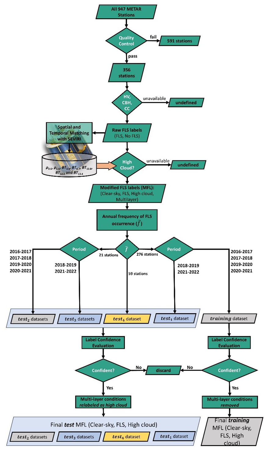
Figure A1 Schematic description of the process followed in Sect. 2 for the creation of the MFLs (modified FLS labels) included in the training, test₁, test₂, test₃, and test₄ datasets.

Figure A1 schematically describes the process followed in Sect. 2 for the creation of the MFLs (modified FLS labels) included in the training, test₁, test₂, test₃, and test₄ datasets.

Appendix B: Equations of statistical validation metrics

$$\begin{array}{}\text{(B1)}& {\displaystyle }\text{POD}=N_{\mathrm{TP}}/(N_{\mathrm{TP}}+N_{\mathrm{FN}})\text{(B2)}& {\displaystyle }\text{FAR}=N_{\mathrm{FP}}/(N_{\mathrm{TP}}+N_{\mathrm{FP}})\text{(B3)}& {\displaystyle }\text{PFD}=N_{\mathrm{TN}}/(N_{\mathrm{FP}}+N_{\mathrm{TN}})\text{(B4)}& {\displaystyle }\text{CSI}=N_{\mathrm{TP}}/(N_{\mathrm{TP}}+N_{\mathrm{FN}}+N_{\mathrm{FP}})\text{(B5)}& {\displaystyle }\text{ACC}=(N_{\mathrm{TP}}+N_{\mathrm{TN}})/(N_{\mathrm{TP}}+N_{\mathrm{TN}}+N_{\mathrm{FP}}+N_{\mathrm{FN}})\text{(B6)}& {\displaystyle }\text{BS}=(N_{\mathrm{TP}}+N_{\mathrm{FP}})/(N_{\mathrm{TP}}+N_{\mathrm{FN}})\text{(B7)}& {\displaystyle }d=\left(\right(\text{POD}-\mathrm{1}{)}^{\mathrm{2}}+{\text{FAR}}^{\mathrm{2}}{)}^{\mathrm{0.5}}\end{array}$$

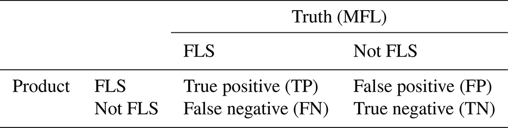
Here N_TP, N_FN, N_FP, and N_TN, respectively, are the number of true positives, false negatives, false positives, and true negatives, as described in Table B1. POD quantifies the skill of the method in correctly identifying the FLS cases. FAR indicates the portion of false alarms among all the cases classified as FLS by the algorithm. PFD highlights the portion of the non-FLS cases which have been correctly classified as non-FLS by the algorithm. CSI is a metric indicating the overall correctness of the FLS classification. ACC shows the portion of the cases which have been correctly identified as FLS and non-FLS. The metrics POD, FAR, PFD, CSI, and ACC vary between 0 and 1. An ideal detection algorithm should have a POD, PFD, CSI, and ACC equal to 1 and FAR equal to 0. BS reflects the overall bias of the product. BS varies between 0 and $+\propto$, with the optimal value being 1. The values of BS greater and smaller than 1 reflect over- and underestimation of the FLS class, respectively. As can be inferred from Eq. (6), d is a metric obtained by combining the statistical indicators POD and FAR and compares the performance of the algorithm with the ideal algorithm (FAR: 0; POD: 1). In other words, it indicates how distant the performance of the FLS detection algorithm is in comparison to that of the best algorithm which can ideally exist. The d value varies between 0 and $\sqrt{\mathrm{2}}$, with 0 being the ideal value.

Table B1 Confusion matrix explaining how the true positives, false negatives, false positives, and true negatives are determined.