SAMURAI-S: Sonic Anemometer on a MUlti-Rotor drone for Atmospheric turbulence Investigation in a Sling load configuration

This study introduces the SAMURAI-S, a novel measurement system that incorporates a state-of-the-art sonic anemometer combined with a multi-rotor drone in a sling load configuration, designed to overcome the limitations of traditional mast-based observations in terms of spatial flexibility. This system enables the direct measurement of 3D wind vectors while hovering, providing a significant advantage in manoeuvrability and positional accuracy over fixed mast setups. The capabilities of the system were quantified through a series of 10 to 28 min flights, conducting close comparisons of turbulence measurements at altitudes of 30 and 60 m against data from a 60 m tower equipped with research-grade sonic anemometers. The results demonstrate that SAMURAI-S matches the data quality of conventional setups for horizontal wind measurements while slightly overestimating vertical turbulence components. This overestimation increases with wind speed.

1 Introduction

Since the 1960s, mast- and tower-based sonic anemometry have been the standard for high-frequency turbulence measurements in atmospheric boundary layer (ABL) research (Foken, 2006; Mauder et al., 2021). With continuous technological development over the years, state-of-the-art sonic anemometers allow for in situ flux estimation (e.g. Foken et al., 2012) and for the spectral characterization (e.g. Midjiyawa et al., 2021) of turbulence. However, several studies in ABL meteorology and wind energy, such as Fernando and Weil (2010), Mahrt (2014), or Veers et al. (2019), highlight the limitations of those traditional tower-based measurements, emphasizing the need for more flexible approaches to address a broader range of relevant ABL processes.

Some examples illustrating mast-based measurement limitations include the study of the coherence of turbulence (Cheynet et al., 2018), a key design parameter for modern wind turbines. For such an investigation, erecting multiple 300 m masts close to each other would be required, which is impractical. The same holds for the detailed investigation of wind turbine wakes within a wind farm, as, for example, explored by Porté-Agel et al. (2020), as variability in wind speed and direction make a proper positioning of masts in such dynamic conditions practically unfeasible. Other research topics that require alternative sensor carriers include the investigation of the wave boundary layer (Wu and Qiao, 2022), air–sea exchange over the ocean (Taylor et al., 2018), and air–ice–sea interactions in polar regions, e.g. over open water areas within the sea ice (Marcq and Weiss, 2012).

Airborne platforms have been used to extend the range of turbulence-related measurements. Fixed-wing uncrewed aerial vehicles (UAVs), often employing multi-hole probes (Mansour et al., 2011; Wildmann et al., 2014a, b; Båserud et al., 2016; Witte et al., 2017; Calmer et al., 2018; Alaoui-Sosse et al., 2019; Rautenberg et al., 2019), have demonstrated their capability in turbulence sampling along the flight track across larger areas. However, the inability to hover or move very slowly restricts their ability to measure in situations requiring stationary point measurements or localized vertical profiling.

Conversely, tethersonde systems equipped with sonic anemometers can provide quasi-stationary measurements and are effective in vertical profiling (Ogawa and Ohara, 1982; Hobby, 2013; Canut et al., 2016). However, those systems require considerable logistical effort and have clear operational limits regarding wind speed and atmospheric turbulence, which strongly affect their controllability. Consequently, tethered systems cannot be easily deployed in remote areas and complex terrain or safely operated near structures and buildings, such as in urban areas or near wind turbines and wind farms.

Rotary-blade UAVs offer a more suitable sensor platform for localized and stationary measurements (Abichandani et al., 2020). Recent studies have explored the use of different methods of atmospheric flow measurements, using either the UAV's motion and attitude as a proxy for wind estimates (Segales et al., 2020; González-Rocha et al., 2020; Shelekhov et al., 2021; Wetz et al., 2021; Wildmann and Wetz, 2022) or by mounting miniaturized sonic anemometers (Palomaki et al., 2017; Li et al., 2023) on the vehicle. Both methods show limitations for turbulence investigations due to the limited sampling frequency and, for most small sonic anemometers, the inability to measure the full 3D flow. First attempts of flying research-grade sonic anemometers (Hofsäß et al., 2019; Thielicke et al., 2021) have shown promising results concerning the measurement of the mean wind speed, but full turbulence measurement capabilities are still unproven.

One main reason is that the propeller-induced flow (PIF) by the UAV can affect and disturb the on-board flow measurements. Mounting an extension arm to place the wind sensor either to the front (Hofsäß et al., 2019), to the side, or above the drone (Thielicke et al., 2021) is one obvious possibility to minimize the PIF effect. Any mass placed outside the centre of gravity of the UAV will inevitably compromise flight stability and complicate flight control. Thus, it is necessary to thoroughly investigate and characterize the PIF for appropriate sensor placement considerations (Ghirardelli et al., 2023; Jin et al., 2024; Flem et al., 2024). The second option, which mitigates the potential PIF influence on the measurements without significantly impacting flight control and stability, is to deploy the flow sensor as a sling load under the drone.

Based on the latter concept, this study introduces SAMURAI-S (Sonic Anemometer on a MUlti-Rotor drone for Atmospheric turbulence Investigation in a Sling load configuration) as a novel measurement system for airborne atmospheric research using drones. To the authors' knowledge, this represents the first attempt to deploy a research-grade sonic anemometer as a suspended payload under a UAV, in contrast to the conventional approach of mounting such instruments rigidly to the UAV structure at relatively short distances (typically on the order of decimetres to a metre), as in the studies above.

Carrying the turbulence sampling payload 18 m under a rotary-wing UAV, the sensor is located outside any measurable PIF effect (Flem et al., 2024). The payload consists of a sonic anemometer, an inertial navigation system (INS), a data acquisition unit, and a mounting frame. This design aims to overcome the limitations mentioned above, thus providing state-of-the-art sonic anemometry data with the added benefits of mobility, hover capability, and adaptable positioning. This will enable detailed turbulence analysis in various settings, including observations close to structures and in urban environments where other methods fail.

This research aims to assess the accuracy and reliability of the developed measurement approach. The methodology involves a comparative analysis between traditional mast-mounted 3D sonic anemometers and the one suspended under the drone. Another key aspect of this study is to evaluate the applicability of a dynamic tilt and motion compensation algorithm to account for the inevitable motion of the payload caused by wind drag and the drone's movements. This algorithm utilizes in situ velocity and attitude data linked to the movement and orientation of the anemometer recorded by the INS. It aims to convert sonic anemometer turbulence measurements obtained from a moving platform to a natural wind or streamline coordinate system, as commonly used in ABL research.

The paper is organized as follows. Sect. 2 details the design of the UAV payload system. Section 3 introduces the algorithm developed to account for the payload motion. This section also outlines the data post-processing techniques employed in the experimental comparison. Section 4 describes the experimental design for system validation, including the measurement site and the setup of the mast instrumentation. Section 5 compares the integral and spectral flow characteristics derived from the mast- and drone-mounted sonic anemometers. Finally, Sect. 6 summarizes the main findings of the study and concludes that SAMURAI-S provides a novel airborne instrument platform with a great potential for effectively measuring ambient turbulent flow with unprecedented flexibility.

2 The SAMURAI-S system

2.1 Airframe

Several important design criteria guided the selection of an appropriate airframe. Turbulence measurement with a drone-mounted sonic anemometer requires lifting a payload of roughly 4 kg. This weight estimate results from the required components, i.e. a research-grade sonic anemometer, an inertial navigation system (INS), a battery, a data logger, and a mounting frame. A flight time of at least 15 to 20 min is required to collect turbulent flow time series that allow robust turbulence statistics for variances and covariances, as well as spectral analysis (Van der Hoven, 1957; Kaimal and Finnigan, 1994). Finally, to comply with European regulations for drone operations in the open category, we wanted to limit the UAV's maximum take-off weight (MTOW) to 25 kg, which also aids the logistical aspects of deploying the system in the field. At the same time, we considered flight safety, stability, and precision in positioning design priorities since they are crucial in different real-world scenarios, such as operations near infrastructure, human presence, or complex environments.

To address these considerations, we opted for the Foxtech D 130 (Fig. 1).

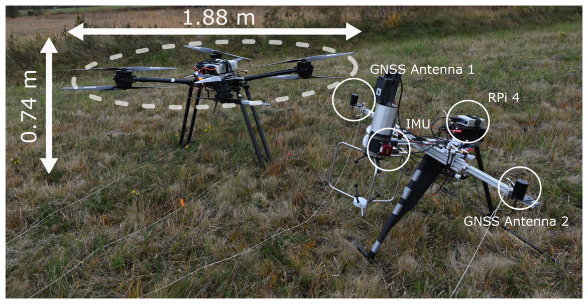
Figure 1 The SAMURAI-S system, showing the Foxtech D130 octocopter (left) and the sampling payload (right). The D130 is an ×8 configuration UAV measuring approximately 1.9 m × 0.7 m. The payload features a cross-shaped aluminium frame, with a longer arm (0.9 m) supporting two Here3 GNSS antennas and a shorter arm (0.6 m) holding an RM Young 81000 ultrasonic anemometer (mounted upside down) and a Raspberry Pi 4 powered by a dedicated power bank. An inertial measurement unit (IMU) is positioned on the side of the anemometer. Key components of the payload are highlighted in the figure.

This UAV has a nominal maximum payload of 20 kg and a maximum flight time in hovering mode of up to 45 min without payload, depending on the atmospheric conditions. It is equipped with eight coaxial contra-rotating propellers, where four pairs of propellers, each driven by brushless electric motors, share the same rotational axis and are mounted on arms extending from the main body (×8 configuration). The configuration of the propellers provides redundancy in case of a motor failure. The frame of the UAV weighs approximately 9 kg. In its default configuration, it is powered by two 6S lithium polymer (LiPo) batteries, each with a capacity of 22 Ah, resulting in a take-off weight of roughly 15 kg excluding the sensor payload. The UAV mounts a CubePilot Cube Orange autopilot unit combined with two global navigation satellite system (GNSS) antennas (Here3). The inclusion of an open-source autopilot unit in the Foxtech D130's standard configuration, combined with its modular design that supports customization and easy rebuilding, ultimately led us to select this model over other alternatives available on the market. The UAV's specifications are shown in Table 1.

Table 1 Specifications of the Foxtech D130.

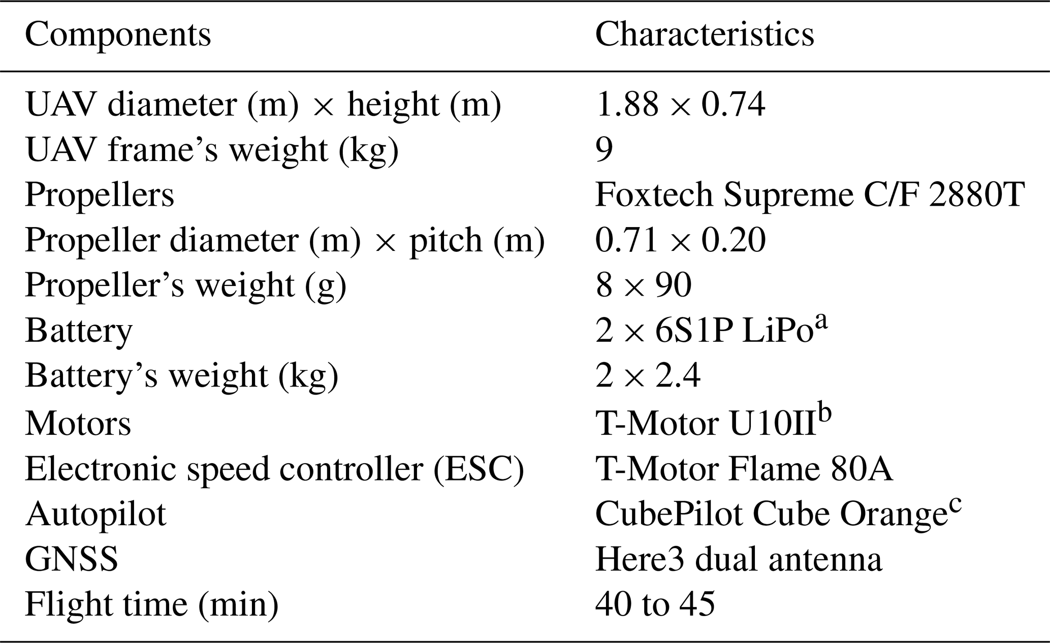
^a 22 Ah; 22.2 V; 30C. ^b 8.6 kg maximum thrust when paired to Foxtech Supreme C/F Propeller 2880T. ^c ArduCopter v4.3.6 in August and v4.4.3 in December.

2.2 Sensor placement

The placement of the sonic anemometer is critical for the quality of the turbulence observations, as it has been shown that placing the sensor at a certain distance from the propellers effectively reduces the impact of the PIF (Prudden et al., 2016; Thielicke et al., 2021; Wilson et al., 2022). However, this approach requires identifying the volume significantly affected by the PIF, which varies with the UAV's geometry (Guillermo et al., 2018; Lei and Cheng, 2020; Lei et al., 2020). Moreover, the angular momentum resulting from the additional weight mounted outside the UAV's centre of gravity could significantly compromise flight stability.

To limit the influence of the PIF on velocity measurements, sensors mounted on a boom above the mean rotor plane of UAVs have been used in the past (Palomaki et al., 2017; Shimura et al., 2018; Natalie and Jacob, 2019; Thielicke et al., 2021; Wilson et al., 2022). This mounting configuration is designed to achieve an evenly balanced weight distribution around the drone by aligning the sensor's weight with the UAV's vertical axis and centre of mass. Nevertheless, this point is true primarily in low wind conditions. In scenarios with stronger winds, the drone must tilt further to counteract the increased drag, affecting the initial balance and tilt angle. Finding the right boom length that effectively reduces PIF while maintaining the drone's manoeuvrability and determining its best orientation remains a subject of ongoing research.

Previous studies (Ghirardelli et al., 2023; Jin et al., 2024), based on the Foxtech D130, suggest that the best trade-off between boom length and PIF reduction while keeping the payload close to the UAV's fuselage is achieved by positioning the boom upwind, with the sensor at the boom's end. This orientation avoids the areas significantly affected by the PIF as shown by Ghirardelli et al. (2023). However, to fully take advantage of this configuration, it is necessary to automatically align the sensor or UAV with the mean instantaneous wind direction, i.e. requiring an automatic flight control loop such as the “weathervaning” algorithm recently implemented in ArduCopter v4.4.0 (see https://ardupilot.org/copter/docs/weathervaning.html, last access: 7 May 2025) or through adjustments in forward flight. To the authors' knowledge, a reliable prototype of this design has yet to be developed.

In this study, we present a novel approach, carrying the sonic payload platform as sling load 18 m under the drone, corresponding to about 26 rotor diameters (D). This setup places the payload in a stable equilibrium state instead of mounting it above the drone. When the payload is suspended beneath the drone, it creates a pendulum, swinging around the point of minimal potential energy. This natural stability allows the payload to stabilize itself through its oscillations, reducing the need for the drone to actively counteract these movements. The PIF features depend more on thrust rather than UAV's geometry in the far field of the drone, i.e. in a distance of more than 5D from the rotor plane, when the individual rotor downwash regions have merged to one (Ghirardelli et al., 2023; Flem et al., 2024). This should extend the applicability of the payload setup to a wider range of multi-copter platforms.

Simulations and observations were used to estimate the required vertical displacement of the wind sensor below the UAV. As detailed in Ghirardelli et al. (2023), simulations within a domain extending 9.0 m below the drone revealed that the ambient wind effectively carries away the downdraughts. Notably, airflow closely resembled free-flow conditions at this domain's lower boundary, directly under the drone and where wind speeds surpassed 2.5 m s⁻¹. This observation was further supported by Jin et al. (2024), which utilizes a configuration of three continuous-wave (CW) Doppler lidars to measure the PIF generated by the Foxtech D130 in hover mode. The measurements indicated a negligible PIF distortion at a distance of 4.5 m below the Foxtech D130, in an ambient flow of 4.0 ms⁻¹. Finally, Flem et al. (2024) showed how, for the same drone model and in the absence of a background flow, the downdraught drops by more than 40 % in the range between 1.5 to 6 m under the plane of the rotors. An additional empirical confirmation can be derived from visual observations of a multi-rotor drone over the surface of a lake in low wind conditions (Flem et al., 2024), showing that the PIF of the drone does not reach the surface, with the UAV hovering at a height of 15D above the water. To add a margin of safety, we opted to double the distance identified in the computational fluid dynamics (CFD) simulations.

2.3 Payload description

The payload consists of an RM Young 81000 sonic anemometer, an SBG System Ellipse-D inertial navigation system (INS) equipped with two GNSS antennas, and a Raspberry Pi 4 (RPi 4) microprocessor serving as a data logger (Figs. 1 and 2). The SBG Systems Ellipse-D is a compact INS featuring a dual-antenna GNSS receiver. It includes a MEMS-based inertial measurement unit (IMU) and uses an extended Kalman filter (EKF) to fuse inertial and GNSS data. Tables 2 and 3 provide key specifications of the sonic anemometer and the INS, respectively.

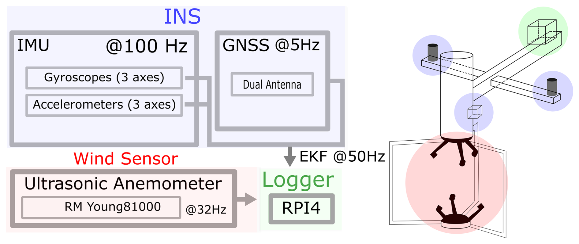
Figure 2 Diagram and blueprint of the measurement and acquisition system showing how data flow from the sensors to the logger. On the left, two main sensor outputs – INS (highlighted in blue) and the ultrasonic anemometer (highlighted in red) – are depicted as being stored and logged by the RPi 4 (highlighted in green). The diagram also indicates the sampling rates, namely 32 Hz for the ultrasonic anemometer and a 50 Hz extended Kalman filter (EKF) output from the INS, which fuses data from a 100 Hz IMU signal and 5 Hz GPS data. On the right, a schematic of the payload shows the physical placement of each component, colour-coded to match the diagram on the left.

Table 2 Specifications of the RM Young 81000 sonic anemometer.

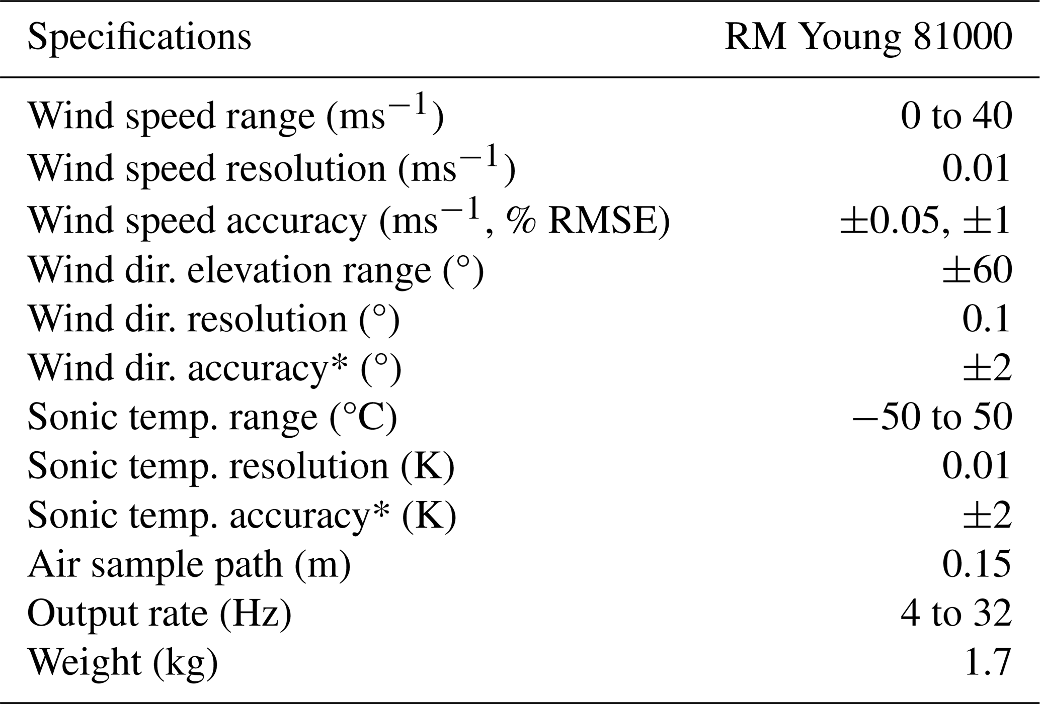
* 0 to 30 ms⁻¹ range.

Table 3 Specifications of the SBG Systems Ellipse-D inertia navigation system with real-time kinematic (RTK) aiding for airborne applications.

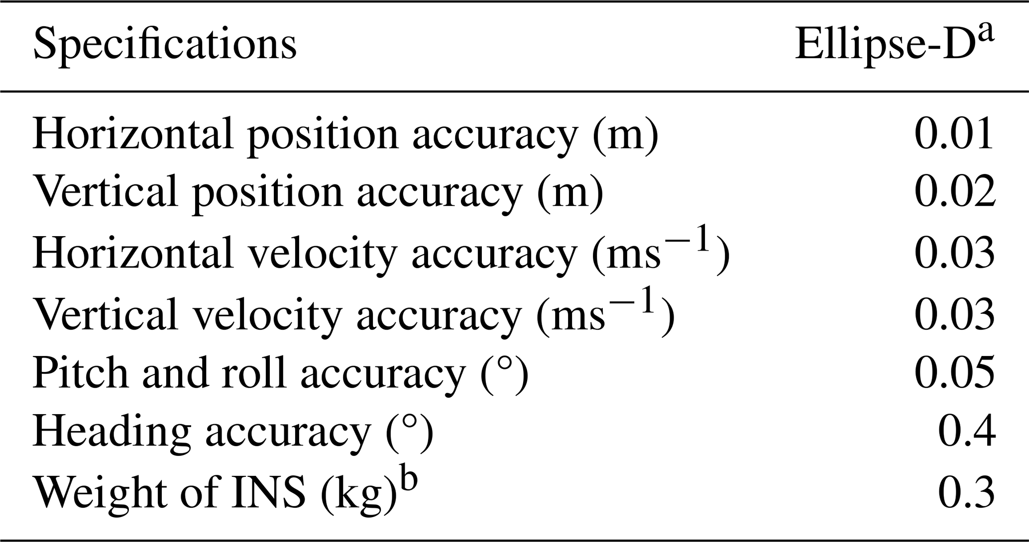
^a Data were logged using the sbgBasicLogger program (sbgECom library v3.2.4011, https://github.com/SBG-Systems/sbgECom, last access: 7 May 2025). ^b including GNSS antennas.

For the integration of the different sensors, the battery, and the data logger, we constructed a horizontal T-shaped aluminium frame with a 0.55 m long main bar and a 1 m long crossbar. In addition, we added a T-shaped support leg to better protect the sensors during landing, transport, and storage and a triangular wind vane to aid the sensor alignment with the mean wind direction and dampen lateral and rotational oscillations around the yaw axis.

The sonic anemometer was mounted upside down in the front of this frame, with the INS attached via a custom-fitted mounting plate to the side of its cylindrical support structure, assuring parallel alignment of both sensor coordinate systems. The crossbar of the frame served as an attachment point for two nylon ropes used to link the payload to the sides of the UAV and a 0.94 m long baseline for the two GNSS antennas mounted on the tips of the bar. The data logger and a battery were positioned at the tail of the frame.

The attachment points for the ropes were aligned with the pitch axis of both the UAV and the sling load (SL) frame. The entire payload system was balanced for the sonic anemometer's pitch by shifting the position of the crossbar, the battery, and the data logger. According to this payload design and placement, the roll motion is directly transferred to the sonic anemometer from the drone, whereas the yaw motion results from a combination of the drone’s dynamics and aerodynamic drag, and the pitch depends mainly on the payload balance. Although the drone–payload setup behaves like a compound pendulum due to the two suspension ropes attached to the same weight (the payload), it has been treated as a simple pendulum for simplicity. The natural oscillation period (T) is estimated using the formula $T=\mathrm{2}\mathit{\pi }\sqrt{\frac{l}{g}}$, where l is the length of the ropes, and g=9.81 ms⁻² is the gravitational acceleration. This calculation yields an oscillation period of approximately 8.5 s, corresponding to a frequency of 0.12 Hz. Preliminary analysis of the sonic data, conducted before performing the motion compensation, consistently revealed a distinct peak at this frequency across all flights.

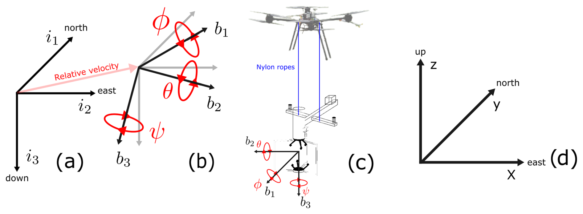
Figure 3 Panel (a) illustrates the inertial frame (NED), where the axes i₁, i₂, and i₃ point northward, eastward, and downward, respectively. Panel (b) depicts the body frame centred at the sonic anemometer’s sampling volume, with axes b₁, b₂, and b₃ pointing forward, to the right, and downward, respectively. This panel also includes the Euler angles ϕ, θ, and ψ depicting the orientation of the body frame relative to the inertial frame, along with the relative velocity vector ${\mathit{V}}_i^b$. Panel (c) illustrates how the payload is attached to the drone by two nylon ropes so that the drone's motion influences the payload’s body frame. This configuration causes the payload to inherit the drone's yaw (ψ) and roll (θ) motions while allowing it to pitch freely. Finally, panel (d) shows the meteorological frame that represents the wind vector U, with eastward, northward, and upward axes.

2.4 Flight operation

The operation of the SAMURAI-S system requires a team of three: a radio control (RC) pilot, a ground control station (GCS) operator, and a payload operator. Before each flight, the UAV and the payload are positioned approximately 10 m apart. The UAV batteries are securely connected, and a telemetry and an RC link are established. The two ropes are attached to two release servos on the UAV, ensuring that they are free of entanglement with the landing gear or ground obstacles. The payload is powered on and held steady to allow proper IMU initialization and gyro calibration. Finally, the operator connects to the RPi 4 Wi-Fi hotspot to verify data streams from the sonic anemometer and the INS, checking for stable GNSS signal and EKF solutions.

During take-off, the payload operator holds the payload steady while the RC pilot executes a vertical ascent to an altitude of approximately 10 m, ensuring that the ropes lift freely without entanglement. Once the ropes are taut, the payload operator releases the payload, and the RC pilot increases the ascent speed. From this point onward, the flight typically continues in auto mode, following a predefined flight plan, including an algorithm to actively adjust the UAV's heading to face the wind (weathervaning).

Throughout the flight, the GCS operator monitors the system's performance and payload data as long as the Wi-Fi connection to the RPi 4 is maintained. After completing the programmed flight plan, a return-to-launch (RTL) command can be triggered automatically or by the RC pilot. In addition, other fail-safe mechanisms, including low battery, are set to trigger an automatic RTL command based on preset conditions.

During landing, the RC pilot takes control as the UAV approaches the landing area, while the payload operator prepares to catch the payload. During the initial fast descent phase, the UAV is flown diagonally to avoid potential stability issues, such as the vortex ring state (Chenglong et al., 2015; Talaeizadeh et al., 2020). The UAV then descends slowly, with the pilot counteracting any swaying of the payload to ensure a smooth catch. Once the payload is secured, the GCS operator releases the ropes via the servos. The RC pilot then increases the distance between the UAV and the payload before initiating the final landing phase. When the UAV is landed, the payload is placed on the ground, and the data acquisition is stopped. After each flight, the data from the payload and flight controller are downloaded and quickly checked, the UAV and payload are powered off, and the batteries are recharged for future flights.

The system consistently performs excellently, showing no stability issues during the flight, take-off, or landing phases, even under strong wind conditions of up to 15 ms⁻¹.

3 Payload data processing workflow

This section outlines the methodological approach to convert the raw flow data sampled by the payload into the natural wind vector expressed in the standard meteorological coordinate system. One primary challenge is handling asynchronous raw sensor output expressed in different coordinate frames. In addition, it is necessary to compensate for the motion of the payload. The workflow presented herein addresses both points through a three-stage process. First, the sonic and INS outputs were filtered to remove faulty data and outliers. Next, these outputs were synchronized, creating a unified temporal framework. Finally, dynamic rotational and translatory transformations were applied to account for changes in the orientation of the payload and its movements, which primarily come from swinging motions during hovering. For clarity, we first introduce the reference systems, which describe the coordinates in which the data are collected and the rotations performed.

3.1 Wind vector, coordinate frames, and transformation

We here define two right-handed coordinate systems to describe the motion of the payload: the inertial frame and the body frame, denoted by the indices i_n and b_n ($n=\mathrm{1},\mathrm{2},\mathrm{3}$), respectively. The inertial (or NED) frame is Earth-fixed, and its axes (i₁, i₂, i₃) are oriented northward, eastward, and downward, respectively (Fig. 3a). The body frame is centred at the sonic anemometer's sampling volume and moves along with the payload. Its axes are defined based on the geometry of the payload, with b₁ pointing forward, b₂ to the right side, and b₃ downward (e.g. Palomaki et al., 2017). Its orientation (attitude) and movements relative to the inertial frame can be described by the Euler angles and the velocity vector measured by the INS, respectively (Fig. 3b).

To transform the raw flow measurements from body frame coordinates (V_b) to inertial frame coordinates (V_i), a rotation matrix $R(\mathit{\varphi },\mathit{\theta },\mathit{\psi })$ is applied (Beard and McLain, 2012; Wetz et al., 2021). This matrix, defined by the roll, pitch, and yaw angles (ϕ, θ, and ψ), adjusts the raw wind vector to reflect the orientation of the payload relative to the inertial frame and is fully detailed in Appendix A. By subtracting the relative velocity vector ${\mathit{V}}_i^b$, accounting for the movement of the body frame relative to the inertial frame, it is possible to eliminate any component of the velocity due to the motion of the payload, isolating the natural wind vector in the inertial frame. The equation that accounts for both of these dynamic corrections is expressed as

$$\begin{array}{}\text{(1)}& {\mathit{V}}_i=R(\mathit{\varphi },\mathit{\theta },\mathit{\psi }){\mathit{V}}_b-{\mathit{V}}_i^b.\end{array}$$

A final orthogonal rotation by right angles is needed to retrieve the wind vector (U) in the standard meteorological coordinate frame, the natural wind coordinate system, with x, y, and z pointing east, north, and up, respectively (Fig. 3c).

$$\begin{array}{}\text{(2)}& \mathit{U}=\left(\begin{array}{ccc}\mathrm{0}& \mathrm{1}& \mathrm{0}\\ \mathrm{1}& \mathrm{0}& \mathrm{0}\\ \mathrm{0}& \mathrm{0}& -\mathrm{1}\end{array}\right){\mathit{V}}_i\end{array}$$

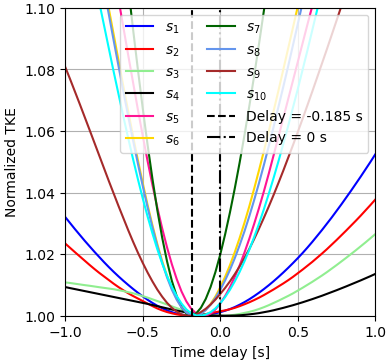
Figure 4 Normalized turbulent kinetic energy (TKE) curves across validation flights (named s₁ to s₁₀) plotted as a function of time delay (in seconds) of the sonic anemometer output relative to the INS output. Each TKE profile is normalized by its minimum value to facilitate direct comparisons. Vertical lines at −0.185 s (dashed line) and 0 s (dot-dash line) indicate the time window where all minimum values are located. The axis limits are set to −1 to 1 for the x axis and 1 to 1.1 for the y axis to highlight subtle differences among the profiles.

3.2 Data filtering

The sonic anemometer, providing the three wind velocity components and the sonic temperature, was set to a sampling frequency of 32 Hz. Each data instance was timestamped according to the RPi 4 internal clock. Since the RPi 4 does not have a GNSS signal, the internal clock does not necessarily correspond to the exact UTC. Therefore, these timestamps were converted to microseconds (µs) from the start of the logging interval, using the first recorded timestamp as an offset.

The raw INS output consists of 100 Hz IMU data and 5 Hz GNSS data. The IMU provides angular rates (gyroscope data) and accelerations (accelerometer data), while the GNSS supplies the local velocity, latitude, longitude, altitude, and roll and yaw angles. Furthermore, the INS outputs EKF data at 50 Hz, fusing inputs from both GNSS and IMU. It consists of 3D velocity data and Euler angles, both given in the NED inertial frame, as well as latitude, longitude, and altitude data. Given the prototype nature of the developed system, the data processing was exclusively based on the EKF output (Table 3).

Moreover, the SBG Ellipse-D INS allows the output of position, velocity, and attitude data at a geometrically specified location relative to the sensor. For convenience, we thus configured the INS to output data in the body frame centred on the sonic anemometer measurement volume. Each data point from the INS was timestamped with the INS internal time in nanoseconds from the start of the data log and in UTC post-GNSS signal acquisition. Figure 2 shows a schematic representation of the payload system.

Before any steps in the filtering workflow, the raw time series were adjusted to account for the sonic anemometer's upside down mounting orientation. This ensured the measured vectors were appropriately rotated in the body frame coordinates.

As an initial filter, we removed all data collected before establishing a valid and stable GNSS time. Following this, data points exceeding the measurement range of the instruments were discarded from further analysis. The filtering thresholds were determined based on the sensor specifications provided by the manufacturers. Additionally, following a despiking method adopted from Mauder et al. (2013), outliers were removed using a moving absolute deviation (MAD) filter relying on a sliding window of 10 s and a distance of ±7 MAD from the median. The combined number of missing and flagged points, following this procedure, did not exceed 2 % in any flight dataset. Thus, they were filled using linear interpolation. The third and final step of the filtering process consisted of identifying the time windows corresponding to the hovering state of the drone. This involved a two-step filtering approach. Initially, a filter was applied based on the median altitude ±3 m, followed by a ±4 m median filter on horizontal movements to address horizontal swinging. Finally, the EKF output was downsampled to 32 Hz to match the sampling frequency of the sonic anemometer via linear interpolation.

3.3 Data synchronization and coordinate transformation

Ensuring accurate synchronization between the INS and the sonic anemometer outputs is crucial for correctly applying Eq. (1), designed to compensate for payload motion during flight. To address potential synchronization discrepancies, we implemented an iterative process that involves progressively changing the time lag of the sonic anemometer relative to the INS within a range of ±2 s, with each step corresponding to $\mathrm{1}/\mathrm{32}$ s. At each adjustment step, Eq. (1) was applied to the sonic data, and we calculated the mean turbulent kinetic energy (TKE) from the resulting time series, defined as

$$\begin{array}{}\text{(3)}& \mathrm{TKE}={\displaystyle \frac{\mathrm{1}}{\mathrm{2}}}\left({\mathit{\sigma }}_u^{\mathrm{2}}+{\mathit{\sigma }}_v^{\mathrm{2}}+{\mathit{\sigma }}_w^{\mathrm{2}}\right).\end{array}$$

Notably, the TKE as a function of the time lag consistently shows a reversed bell shape with the minimum located between −0.185 to 0 s, as shown in Fig. 4.

Apart from the location of the time lag, this figure also indicates that potential errors associated with an imperfect time-lag correction, e.g. by a few time increments, would result in small relative errors in the computed TKE.

The time series adjusted using the time lag that minimizes the TKE were selected for further analysis. This selection was based on the assumption that the payload movement is most effectively compensated at this optimal lag. Finally, these time series were transformed into natural wind coordinates using Eq. (2).

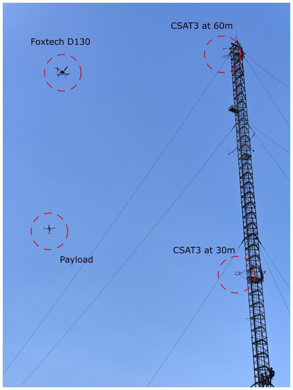
Figure 5 SAMURAI-S hovering side by side with the reference mast. The two CSAT sonic anemometers are mounted at 30 m and 60 m a.g.l., oriented towards 218.0 and 230.5 °, respectively.

4 Data and methods for the validation experiment

The validation study was conducted at the Plateforme Pyrénéenne d'Observations Atmosphériques (P2OA) in Lannemezan, southwestern France, during two special observation periods in August and December 2023, as part of the Model and Observation for Surface Atmosphere Interactions (MOSAI) campaign. During these periods, the SAMURAI-S, reusable radiosondes, multiple eddy-covariance stations, meteorological masts, and various remotely piloted aircraft systems were used to study the effects of surface heterogeneities on the local wind conditions. Additionally, a tethered balloon equipped with a sonic anemometer (Canut et al., 2016) provided a complementary method for assessing atmospheric turbulence. While this constitutes an important experimental dataset, the current work focuses solely on validating the SAMURAI-S system. Detailed analysis of the scientific data from the experimental campaign is reserved for future publications.

The P2OA observatory is located in a rural and heterogeneous area, characterized primarily by agricultural fields and forests, with a typical length scale of 500 m (e.g. BLLAST; Lothon et al., 2014). The site has a 60 m meteorological tower with a triangular lattice structure (Fig. 5). The terrain around the tower is predominantly flat and is characterized by a heterogeneous mix of grazing land, grasslands, crop fields, and forest. Within 1 km of the 60 m tower, grasslands are more prevalent.

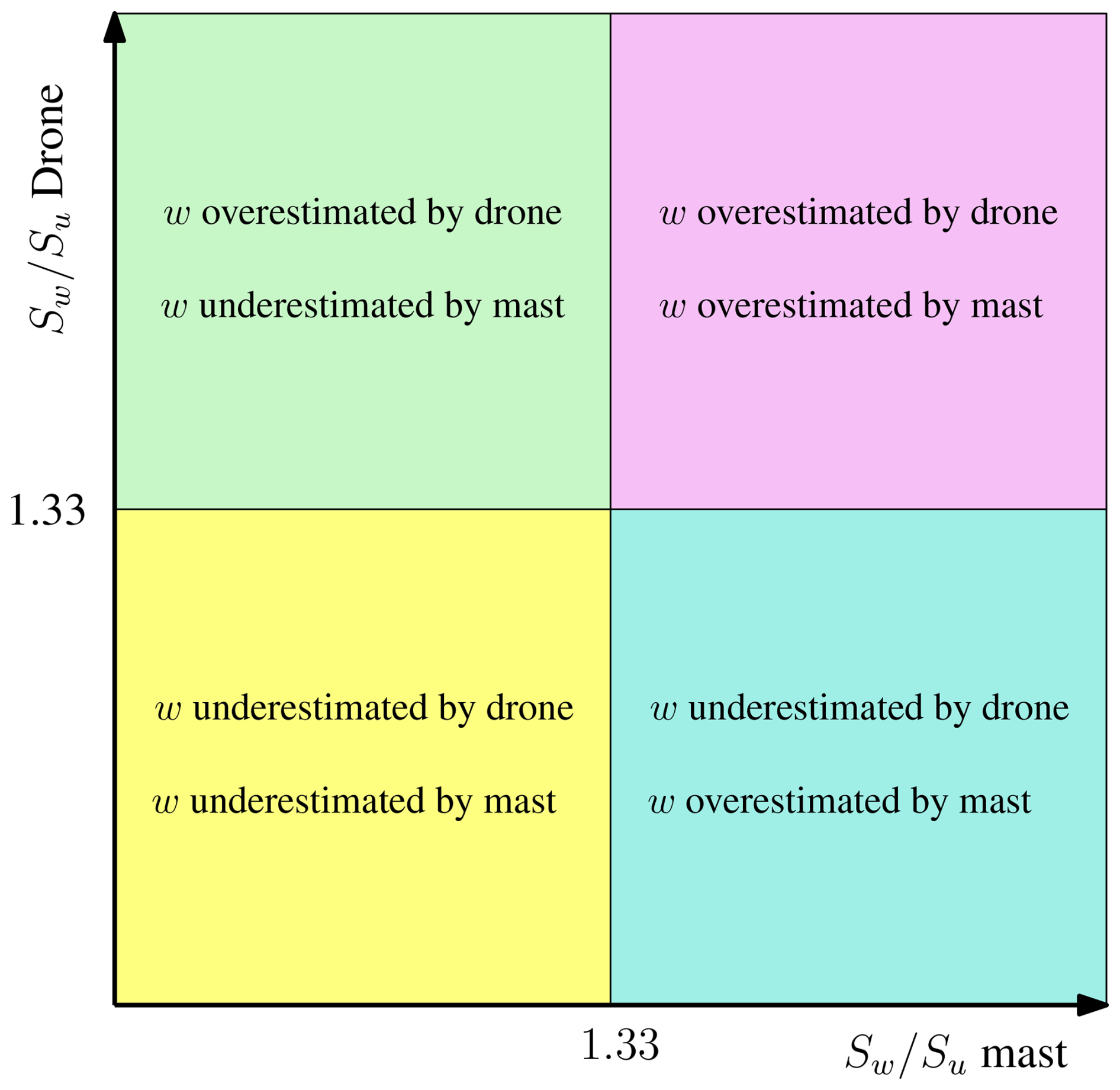
Figure 6 Quadrant analysis of the spectral ratios $S_w/S_u$ to identify which sensor configuration may overestimate or underestimate the vertical velocity component. For brevity, “drone” refers to the drone-mounted sonic anemometer in this figure, and “mast” refers to the mast-mounted sonic anemometer.

The tower is equipped with slow-response sensors for temperature, humidity, wind speed, and direction at five levels (2, 15, 30, 45, and 60 m) and eddy-covariance systems at three levels (30, 45, and 60 m), of which only the lowermost and uppermost systems were operational during our validation period. Two Campbell Scientific CSAT3 sonic anemometers were mounted on horizontal booms on the tower at heights of 30 and 60 m above the ground (633 and 663 m above mean sea level), with an azimuth of 218.0 and 230.5 °, respectively. These anemometers operated with a sampling frequency of 10 Hz, recording the three velocity components and the sonic temperature. The validation study described herein comprises several hovering flights of SAMURAI-S at target altitudes of 30 and 60 m near the mast.

Table 4 Summary of the 10 samples assessed in this study.

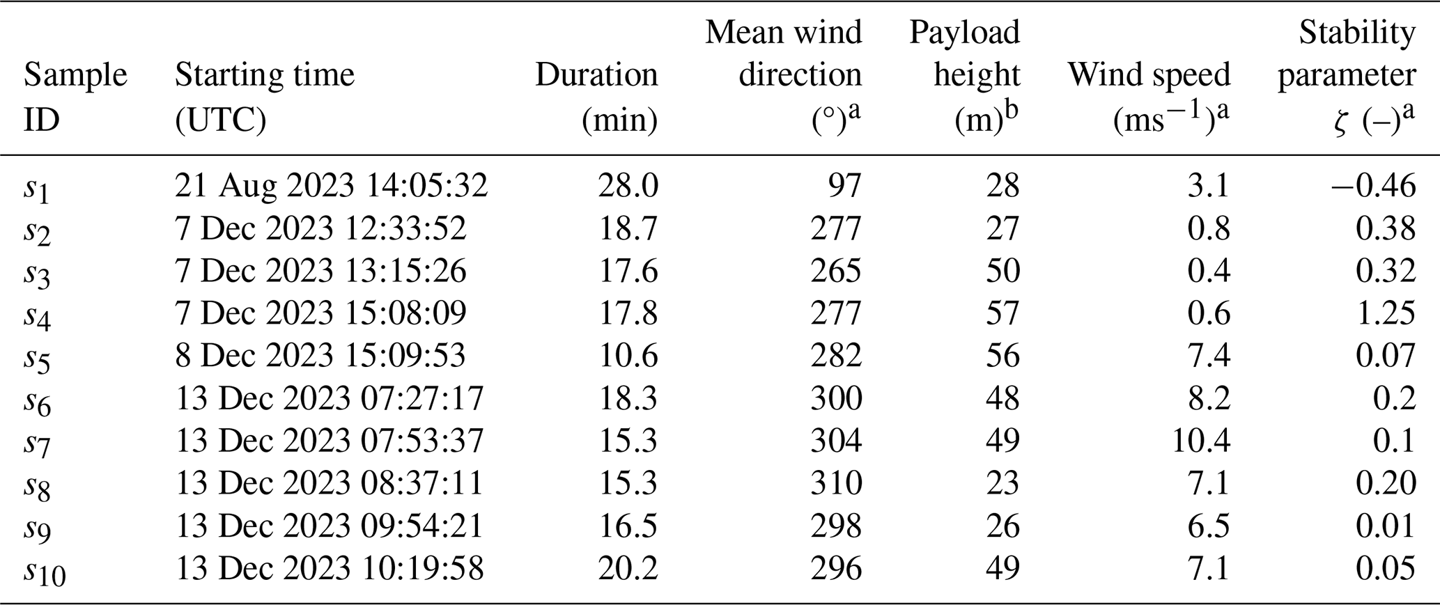
^a Value estimated by the mast-mounted sonic anemometer closest to the payload height during the hovering window. ^b Average height of the drone during the hovering window.

4.1 Tower validation study: theoretical framework

For this validation study, we express the wind vector U in a coordinate system that is aligned with the mean flow streamlines (Kaimal and Finnigan, 1994). In this coordinate system, the three velocity components (u, v, and w) correspond to the along-wind, across-wind, and vertical (upward) directions, respectively. We apply Reynolds decomposition, splitting each component $i=u,v,w$ into a mean part, $\stackrel{\mathrm{‾}}{i}$, and a fluctuating part, i^′. The fluctuating component with a zero mean is treated as a stationary, homogeneous, ergodic, and Gaussian random process. The standard deviations of the u, v, and w components are represented by σ_u, σ_v, and σ_w. Additionally, the skewness and kurtosis of these components, which quantify the deviation from the assumption of Gaussian fluctuations, are denoted by γ_i and κ_i.

This study utilizes the blunt and pointed spectral models (Olesen et al., 1984; Tieleman, 1995) to examine whether the velocity spectra conform to the $-\mathrm{5}/\mathrm{3}$ power law in the inertial subrange. The models are a good approximation of the turbulence spectra in the atmospheric surface layer. In this study, they are expressed in their dimensionless form as

$$\begin{array}{}\text{(4)}& {\displaystyle \frac{f{S}_u\left(f\right)}{u_{*}^{\mathrm{2}}}}={\displaystyle \frac{a_u{f}_r}{{\left(\mathrm{1}+b_u{f}_r\right)}^{\mathrm{5}/\mathrm{3}}}},\text{(5)}& {\displaystyle \frac{f{S}_v\left(f\right)}{u_{*}^{\mathrm{2}}}}={\displaystyle \frac{a_v{f}_r}{{\left(\mathrm{1}+b_v{f}_r\right)}^{\mathrm{5}/\mathrm{3}}}},\text{(6)}& {\displaystyle \frac{f{S}_w\left(f\right)}{u_{*}^{\mathrm{2}}}}={\displaystyle \frac{a_w{f}_r}{\mathrm{1}+b_w{f}_r^{\mathrm{5}/\mathrm{3}}}},\text{(7)}& {\displaystyle \frac{f\mathrm{Re}\left(S_{uw}\left(f\right)\right)}{u_{*}^{\mathrm{2}}}}={\displaystyle \frac{a_{uw}{f}_r}{{\left(\mathrm{1}+b_{uw}{f}_r\right)}^{\mathrm{7}/\mathrm{3}}}},\end{array}$$

where a_i and b_i, with $i=\mathit{\{}u,v,w,uw\mathit{\}}$, are coefficients empirically determined, and f_r is a reduced frequency defined as

$$\begin{array}{}\text{(8)}& f_r={\displaystyle \frac{fz}{\stackrel{\mathrm{‾}}{u}}}.\end{array}$$

The Obukhov length (Monin and Obukhov, 1954) can be calculated as

$$\begin{array}{}\text{(9)}& L=-{\displaystyle \frac{u_{*}^{\mathrm{3}}{\stackrel{\mathrm{‾}}{\mathit{\theta }}}_v}{g\mathit{\kappa }\left(\stackrel{\mathrm{‾}}{w^{\prime }{\mathit{\theta }}_v^{\prime }}\right)}},\end{array}$$

where ${\stackrel{\mathrm{‾}}{\mathit{\theta }}}_v$ is the mean virtual potential temperature approximated by the sonic temperature, κ=0.40 is the von Kármán constant, and $\stackrel{\mathrm{‾}}{w^{\prime }{\mathit{\theta }}_v^{\prime }}$ is the buoyancy flux. The non-dimensional stability parameter ζ is defined as $\mathit{\zeta }=z/L$, where z is the height above the surface.

Figure 7 Drone altitude (a) and horizontal position relative to the tower (b) during the measurement periods of the 10 validation flights. The sonic anemometers on the mast are mounted at heights of 30 and 60 m, oriented at 218.0 and 230.5 °, respectively. Wind directions for each flight are shown as coloured arrows, originating from the average horizontal positions. The arrow lengths correspond to a reference vector of 2 ms⁻¹. © Google Earth 2024, using 2024 imagery of Maxar Technologies

Following Kolmogorov's hypothesis of local isotropy in the inertial subrange, the spectral ratios $S_w/S_u$ and $S_v/S_u$ should converge toward $\mathrm{4}/\mathrm{3}$ as the frequency increases (Busch and Panofsky, 1968; Kaimal et al., 1972). To compare the effectiveness of the mast-mounted and drone-mounted sonic anemometers in resolving turbulence with minimal flow distortion, we apply a quadrant analysis based on the comparison of the ratio $S_w/S_u$ between the two sensor configurations (Fig. 6). In the ideal scenario, data points in this figure would cluster around the centre of the plot, as the $\mathrm{4}/\mathrm{3}$ ratio is reached by both the drone- and mast-based data. Deviations from this ratio could indicate flow distortion caused by the supporting structure, the sensor head, or both (Cheynet et al., 2019; Peña et al., 2019). A spectral ratio approaching but not reaching $\mathrm{4}/\mathrm{3}$ may suggest that isotropy in the inertial subrange is not achieved within the investigated frequency range (Chamecki and Dias, 2004). A spectral ratio that plateaus without reaching the $\mathrm{4}/\mathrm{3}$ law may reflect flow distortion, typically manifesting as an underestimation of the vertical velocity component. It should be noted that Kolmogorov's hypothesis of local isotropy in the inertial subrange may not apply under non-stationary conditions, e.g. in very stable atmospheric conditions with intermittent turbulence. Thus, the quadrant analysis was conducted only for samples with a mean wind speed above 2 ms⁻¹, which was sufficient in this study to eliminate samples that did not exhibit characteristics consistent with the framework adopted here to describe turbulence.

In this study, the spectral ratios are studied using a limited frequency range of interest, which is computed using the reduced frequency f_r (Eq. 8), and f_r>2 following Kaimal et al. (1972). An upper boundary f_r<10 is also applied to ensure a fairer comparison between the drone and mast data.

4.2 Statistical uncertainties

The uncertainties associated with turbulent flux measurements are analysed using the methodology described by Wyngaard (1973), Forrer and Rotach (1997), and Stiperski and Rotach (2016). This approach quantifies the random error arising from a fixed averaging period (τ) and the mean wind speed ($\stackrel{\mathrm{‾}}{u}$). Within this framework, the uncertainties in the momentum fluxes (a_uw, a_vw), the buoyancy flux ($a_{w{\mathit{\theta }}_v}$), and those associated with any turbulent variable ξ are expressed as the following non-dimensional quantities:

$$\begin{array}{}\text{(10)}& {\displaystyle }{a}_{uw}^{\mathrm{2}}={\displaystyle \frac{z}{\mathit{\tau }\stackrel{\mathrm{‾}}{u}}}\left({\displaystyle \frac{\stackrel{\mathrm{‾}}{(u^{\prime }{w}^{\prime }{)}^{\mathrm{2}}}}{u_{*}^{\mathrm{4}}}}-\mathrm{1}\right),\text{(11)}& {\displaystyle }{a}_{vw}^{\mathrm{2}}={\displaystyle \frac{z}{\mathit{\tau }\stackrel{\mathrm{‾}}{u}}}\left({\displaystyle \frac{\stackrel{\mathrm{‾}}{(v^{\prime }{w}^{\prime }{)}^{\mathrm{2}}}}{u_{*}^{\mathrm{4}}}}-\mathrm{1}\right),\text{(12)}& {\displaystyle }{a}_{{\mathit{\theta }}_{v}w}^{\mathrm{2}}={\displaystyle \frac{z}{\mathit{\tau }\stackrel{\mathrm{‾}}{u}}}\left({\displaystyle \frac{\stackrel{\mathrm{‾}}{(w^{\prime }{\mathit{\theta }}_v^{\prime }{)}^{\mathrm{2}}}}{(\stackrel{\mathrm{‾}}{w^{\prime }{\mathit{\theta }}_v^{\prime }}{)}^{\mathrm{2}}}}-\mathrm{1}\right),\text{(13)}& {\displaystyle }{a}_{{\mathit{\xi }}^{\mathrm{2}}}^{\mathrm{2}}={\displaystyle \frac{\mathrm{4}z}{\mathit{\tau }\stackrel{\mathrm{‾}}{u}}}\left({\displaystyle \frac{\stackrel{\mathrm{‾}}{{{\mathit{\xi }}^{\prime }}^{\mathrm{4}}}}{(\stackrel{\mathrm{‾}}{{{\mathit{\xi }}^{\prime }}^{\mathrm{2}}}{)}^{\mathrm{2}}}}-\mathrm{1}\right).\end{array}$$

These uncertainties reflect the assumption of ergodicity, which states that the time average converges towards the ensemble average given a sufficiently long averaging period. This assumption is at the core of the turbulence analysis with ultrasonic anemometers. Consequently, these uncertainties are inversely proportional to both the averaging time and the wind speed. Eqs. (10) to (12) are typically associated with greater uncertainties than Eq. (13), as the estimation of covariance requires a longer averaging period than variance estimates (Kaimal and Finnigan, 1994). The relative magnitude of uncertainties also depends on terrain roughness and stability conditions. Following the recommendations of Stiperski and Rotach (2016) and Cheynet et al. (2019), uncertainties below 0.5 indicate high-quality measurements.

4.3 Integral length scales

The integral length scales of turbulence are one-point statistics that quantify the spatial structure of turbulent eddies. These length scales are used both in micrometeorology and wind engineering for structural design. One integral length scale can be defined per velocity component. In this study, the integral length scales were estimated in two steps. First, the integral timescale was determined by fitting an exponential function to the autocovariance function of the velocity fluctuations. The autocovariance function for a given velocity component, ξ, is defined as

$$\begin{array}{}\text{(14)}& {\displaystyle }{R}_{\mathit{\xi }\mathit{\xi }}\left(\mathit{\tau }\right)=\stackrel{\mathrm{‾}}{{\mathit{\xi }}^{\prime }\left(t\right){\mathit{\xi }}^{\prime }(t+\mathit{\tau })},\end{array}$$

where R_ξξ(τ) is the autocovariance function at lag τ. The integral timescale, T_ξ, was then obtained by a least-square fit of an exponential function to Eq. (14):

$$\begin{array}{}\text{(15)}& {\displaystyle }{R}_{\mathit{\xi }\mathit{\xi }}\left(\mathit{\tau }\right)\approx R_{\mathit{\xi }\mathit{\xi }}\left(\mathrm{0}\right)\exp \left({\displaystyle \frac{-\mathit{\tau }}{T_{\mathit{\xi }}}}\right).\end{array}$$

In the second step, Taylor's frozen turbulence hypothesis was applied to convert the integral timescale into the integral length scale. Taylor's hypothesis is generally valid for moderate and low turbulence intensities. Hereinafter, we define turbulence as “frozen” when the following conditions are satisfied:

$$\begin{array}{}\text{(16)}& {\displaystyle }{I}_u={\displaystyle \frac{{\mathit{\sigma }}_u}{\stackrel{\mathrm{‾}}{u}}}<\mathrm{0.5}\text{and}\stackrel{\mathrm{‾}}{u}>\mathrm{1}{\mathrm{m}\mathrm{s}}^{-\mathrm{1}}.\end{array}$$

Under these conditions, the integral length scale, L_ξ, is given by

$$\begin{array}{}\text{(17)}& {\displaystyle }{L}_{\mathit{\xi }}{\displaystyle }=\stackrel{\mathrm{‾}}{u}{T}_{\mathit{\xi }}.\end{array}$$

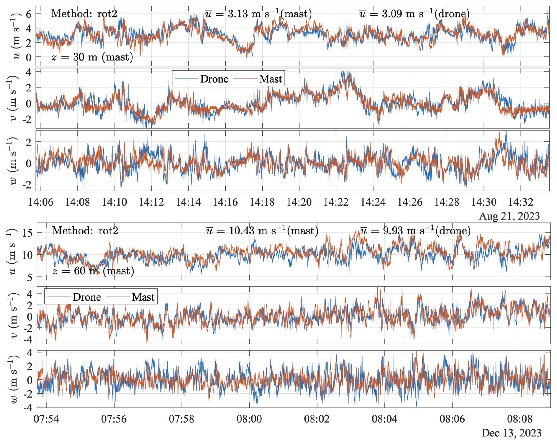
Figure 8 Velocity time series of the wind components: streamwise (u), crosswind (v), and vertical (w), from drone- and mast-based setups during flights s₁ (upper panel) and s₇ (lower panel). The time series from the drone and tower-based setup are coloured blue and orange, respectively. The double rotation (Method: rot2) was applied to both the drone and tower data. The variable z corresponds to the height of the sonic anemometer mounted on the tower, which was the one closest to the drone-mounted sonic anemometer hovering altitude. At the same time, $\stackrel{\mathrm{‾}}{u}$ denotes the average streamwise wind component calculated over the sampling period.

4.4 Data processing

Data from the payload and the mast-mounted anemometers are collected at different locations. Therefore, the same turbulent structures may be detected at slightly different times due to flow advection. To address this, the two datasets are initially synchronized by an automated procedure that iteratively identifies and applies the optimal time shift (up to a maximum of 6 s) that maximizes the cross-correlation of the horizontal velocity fluctuations. The procedure then uses linear interpolation to align the time series and ensure both datasets capture the same turbulent features. Subsequently, the data are downsampled by a factor of 4, and an anti-aliasing finite impulse response (FIR) filter of order 4 is applied. This leads to a sampling frequency of 8 Hz, which was adequate for properly comparing the two datasets.

Misalignments due to small errors in estimating the orientation of the sonic anemometers mounted on the tower or the relative positioning between the INS and the sonic anemometer on the payload can occur. To detect such discrepancies, the datasets from both the payload and the mast (set as the reference) are compared after retrieving the velocity components – namely u, v, and w – using single, double, or triple rotation methods (McMillen, 1988). While the single rotation aligns u with the mean wind direction, the double-rotation method involves an additional pitch rotation, ensuring $\stackrel{\mathrm{‾}}{w}=\mathrm{0}$. In contrast, triple rotation includes a third rotation around the roll axis to ensure the crosswind component of the kinematic momentum flux ($\stackrel{\mathrm{‾}}{v^{\prime }{w}^{\prime }}$) becomes zero. A preliminary comparison involving these three rotations showed limited differences, demonstrating the suitability of the measurement setup. For simplicity, the double-rotation method was chosen for both the mast-mounted and the drone-mounted anemometers for further analysis.

Integral and spectral turbulence characteristics are studied using linearly detrended data. Auto-power spectral densities (PSDs) and cross-power spectral densities (CPSDs) of the velocity and temperature fluctuations are estimated using Welch's method (Welch, 1967). We divided the data into three segments with 50 % overlap. An additional step includes smoothing the PSDs by bin-averaging them over 100 logarithmically spaced bins (Kaimal and Finnigan, 1994).

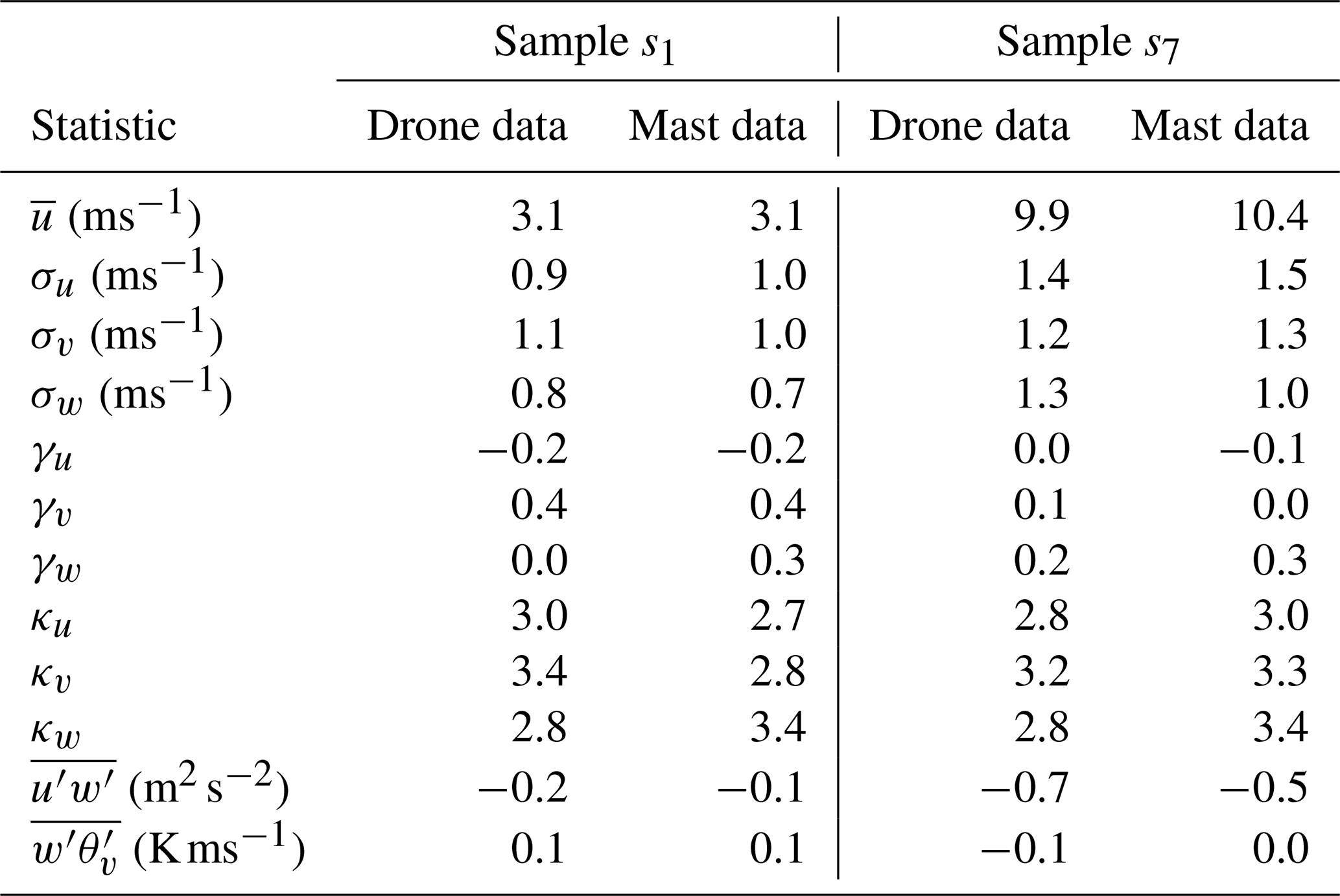
Table 5 Mean and turbulent flow statistics for samples s₁ and s₇ for drone and mast data. Samples s₁ and s₇ refer to the samples described in Table 4. σ_i, γ_i, and κ_i, where $i=u,v,w$, refer to the standard deviation, skewness, and kurtosis estimates, respectively. The table also includes the momentum flux values ($\stackrel{\mathrm{‾}}{u^{\prime }{w}^{\prime }}$) and buoyancy flux values ($\stackrel{\mathrm{‾}}{w^{\prime }{\mathit{\theta }}_v}$).

5 Results and discussion

In this study, we examine a dataset comprising 10 samples, labelled s₁ to s₁₀ in Table 4, to assess turbulence measurements obtained via the drone-mounted sonic anemometer.

These samples were chosen from 17 initial flights, with the selection criteria based on at least 10 min of continuous, high-quality EKF output corresponding to hovering flight. Notably, s₂, s₃, and s₄ have mean flows of less than 2 ms⁻¹. The assumptions of turbulence being stationary, homogeneous, ergodic, and modelled as a Gaussian random process might not hold for these flights, making them unsuitable for the quadrant analysis framework proposed in Sect. 4.1. Nevertheless, they were included in the analysis for the sake of completeness.

Figure 7 shows the associated altitude of the payload above the ground (left panel) and the hovering distance from the tower during the measurement periods (right panel).

Although all flights were analysed, for brevity Sect. 5.1 features a detailed comparison of the exemplary cases from samples s₁ and s₇ as they exhibit markedly different characteristics. Sample s₁ targeted a height of 30 m and features convective conditions ($\mathit{\zeta }=-\mathrm{0.46}$) with rather weak wind of 3.1 ms⁻¹. Conversely, sample s₇, which targeted 60 m, is characterized by stable stratification conditions (ζ=0.1) and the highest wind speed in the series (10.4 ms⁻¹). It will be shown that while s₁ exhibits an excellent correlation between the drone-mounted anemometer and its mast-mounted counterpart, s₇ presents some discrepancies in the vertical component when comparing the two anemometers. Following these detailed examinations, we systematically compare all samples in Sect. 5.2. Finally, we conclude the comparison by presenting flux uncertainties between the drone- and mast-based datasets in Sect. 5.3.

5.1 Cases of samples s₁ and s₇

This section focuses first on the second-order structure of turbulence (i.e. variances and covariances) of s₁ and s₇, as these samples show strongly contrasting characteristics, as pointed out in the previous section. The third and fourth statistical moments (i.e. skewness and kurtosis) are also briefly discussed for completeness. Figure 8 presents time series of the velocity components u, v, and w for samples s₁ and s₇. Results related to temperature are presented separately later in the section.

Table 5 expands on this comparison by showing the statistical moments for the three velocity components between the reference mast data and the SAMURAI-S data.

Flow statistics from the drone- and mast-mounted sensors are in good agreement, except for the vertical velocity component w of sample s₇, where the drone-mounted sonic anemometer shows slightly larger fluctuations (σ_w=1.3 ms⁻¹) than those from the mast-mounted sensor (σ_w=1 ms⁻¹). All three velocity components in the mast and the payload data exhibit skewness and kurtosis values close to zero and three, respectively. These measurements indicate Gaussian fluctuations, typically observed under stationary conditions within the ABL. Despite an 11 m altitude discrepancy between the sensors (see Fig. 7), the drone-mounted sensor accurately tracks short-term horizontal velocity fluctuations. The altitude difference is primarily due to the UAV's altitude control being based on pressure rather than GNSS. Unfortunately, this discrepancy was only noticed during the post-processing phase and was not corrected in the field.

Figure 9 presents the auto-power spectral density (PSD) for each velocity component and the real part of the cross-spectrum between u and w for samples s₁ and s₇, plotted on a log–log scale and multiplied by the frequency f to highlight spectral features.

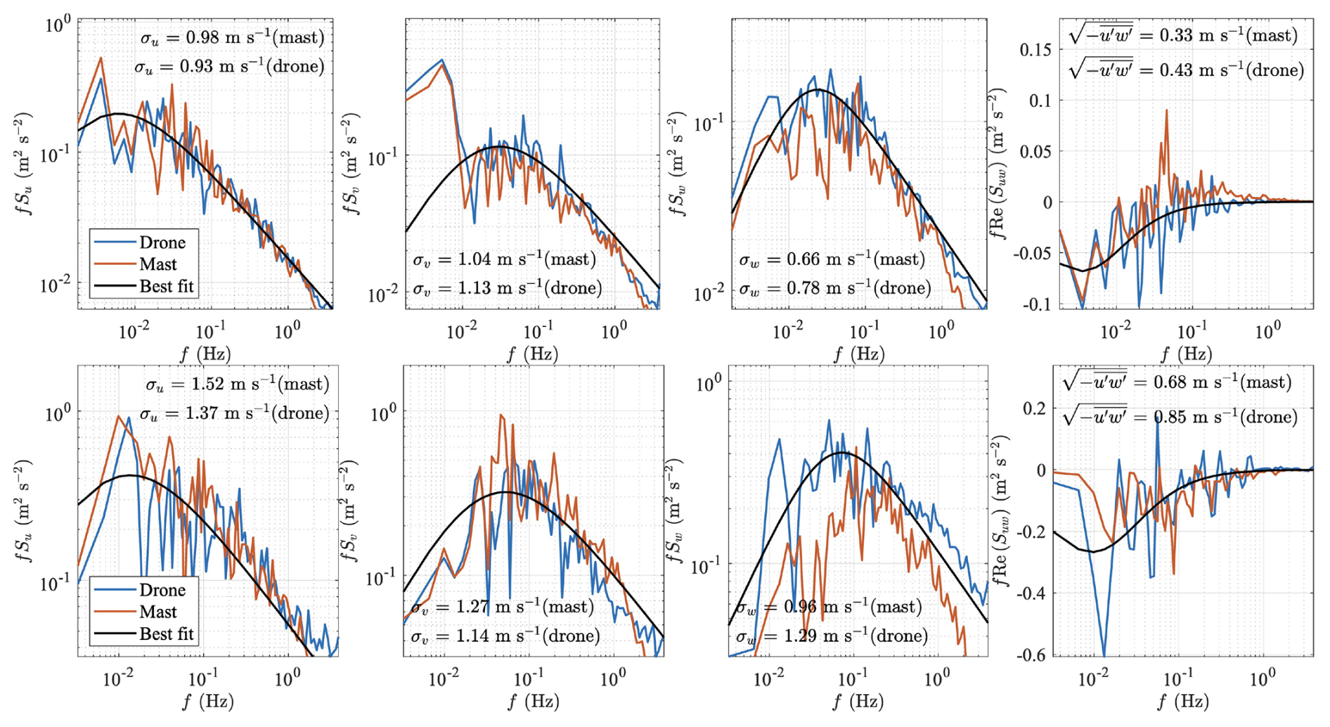
Figure 9 Power spectral density (PSD) estimates of the velocity components: streamwise (u), crosswind (v), and vertical (w), as well as the co-spectrum (Re(S_uw)), from drone- and mast-based setups during flight s₁ (upper panels) and s₇ (lower panels). The solid black line refers to the blunt model (for S_u, S_v, and Re(S_uw)) or pointed model (for S_w) fitted to the data from the drone-mounted anemometer. The variances of the velocity components (σ_u, σ_v, and σ_w) and the Reynolds stress element $\stackrel{\mathrm{‾}}{u^{\prime }{w}^{\prime }}$ are indicated within each corresponding panel.

The smooth PSD is computed using Eqs. (4) to (7) that are fitted to the data recorded by the payload sensor. This least-square fit is useful to assess whether the estimated PSD follows the $-\mathrm{5}/\mathrm{3}$ power law associated with the inertial subrange for the S_u, S_v, and S_w spectra, as well as the $-\mathrm{7}/\mathrm{3}$ power law for the co-spectrum Re(S_uw). A slightly steeper roll-off is observed for the mast data.

Both sensors consistently capture the along-wind (u) and across-wind (v) velocity components for the selected samples s₁ and s₇. In sample s₁, the S_v spectrum reveals a small peak at approximately 0.20 Hz. This peak cannot be attributed to the oscillation frequencies of the payload, which are established around 0.11 Hz. Thus, it is more likely related to random fluctuations. The co-spectrum between u and w for sample s₁ features unusual positive values in the mast-mounted data between 0.03 to 1 Hz, with a distinctive positive peak at 0.04 Hz. These features are not present in the SAMURAI-S data, indicating differences in the flow between those captured by the tower-mounted instrument. This peak is unlikely related to a shadow effect of the tower, given that the wind direction was 97 ° and the tower-mounted sonic sensor is oriented towards 218 ° for s₁.

For flight s₇, the power spectral density of the vertical component clearly shows a higher energy content at all frequencies recorded by the drone-based sonic anemometer compared to those from the tower (Fig. 9). This is consistent with the higher σ_w values from the drone data shown in Table 5. This feature is present in nearly all flights (see Sect. 5.2), although it is particularly pronounced in s₇.

The comparative analysis of the sonic temperature time series reveals a good agreement across sample s₁ and s₇, with minor deviations for the mean temperature likely attributable to different calibration values between the sonic anemometers (Fig. 10).

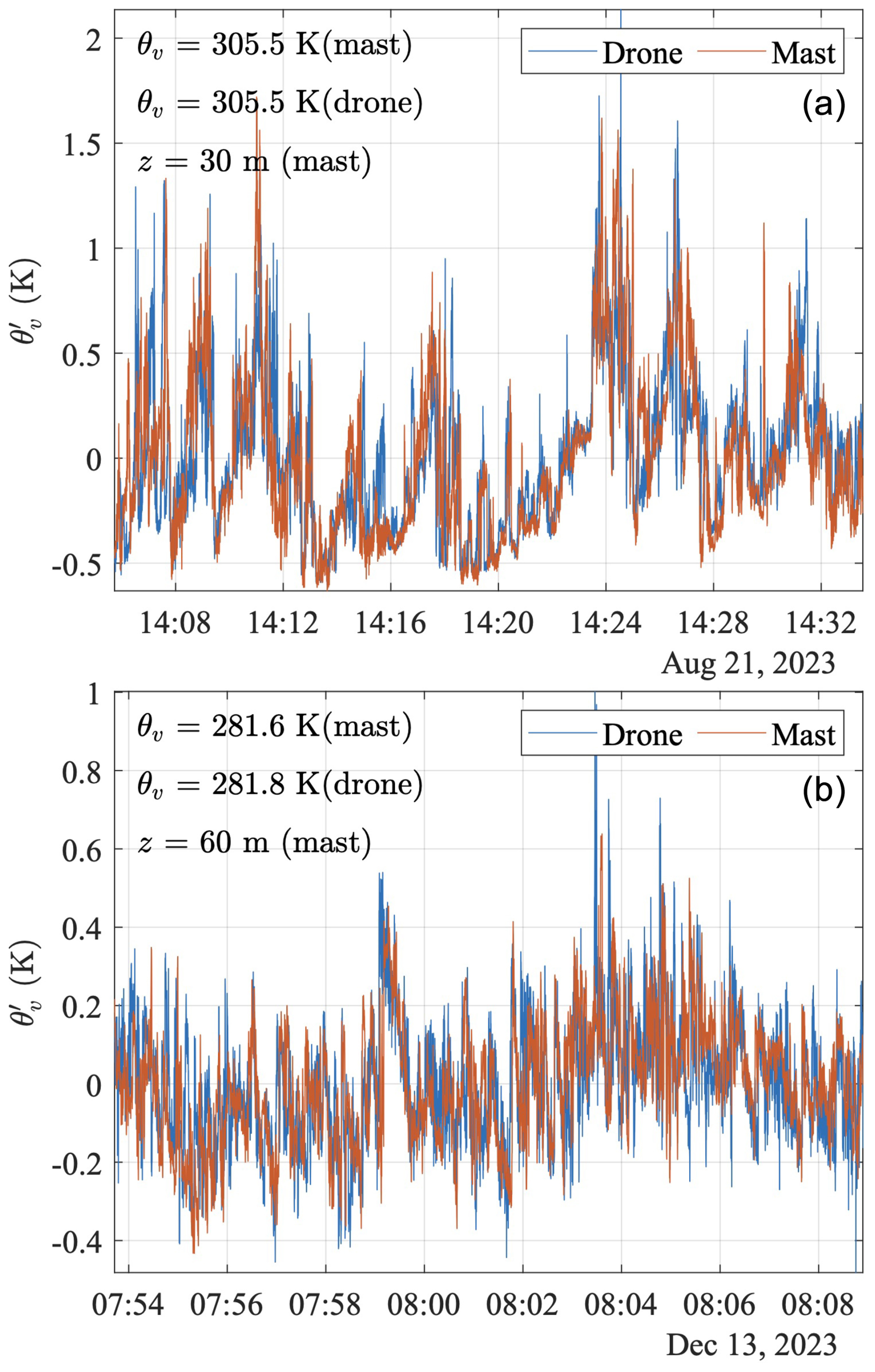
Figure 10 Time series of the fluctuations of the sonic temperature (${\mathit{\theta }}_v^{\prime }$) for samples s₁ (a) and s₇ (b) measured by the drone-mounted anemometer (blue line) and the mast-mounted sonic sensor (orange line) at heights of 30 and 60 m above the ground, respectively. The mean sonic temperature (θ_v) is also indicated in each panel for both the drone and the mast measurements.

Further insights are provided by Fig. 11, which displays the PSD estimates of the sonic temperature and the CPSD between the vertical and the along-wind component with the virtual potential temperature.

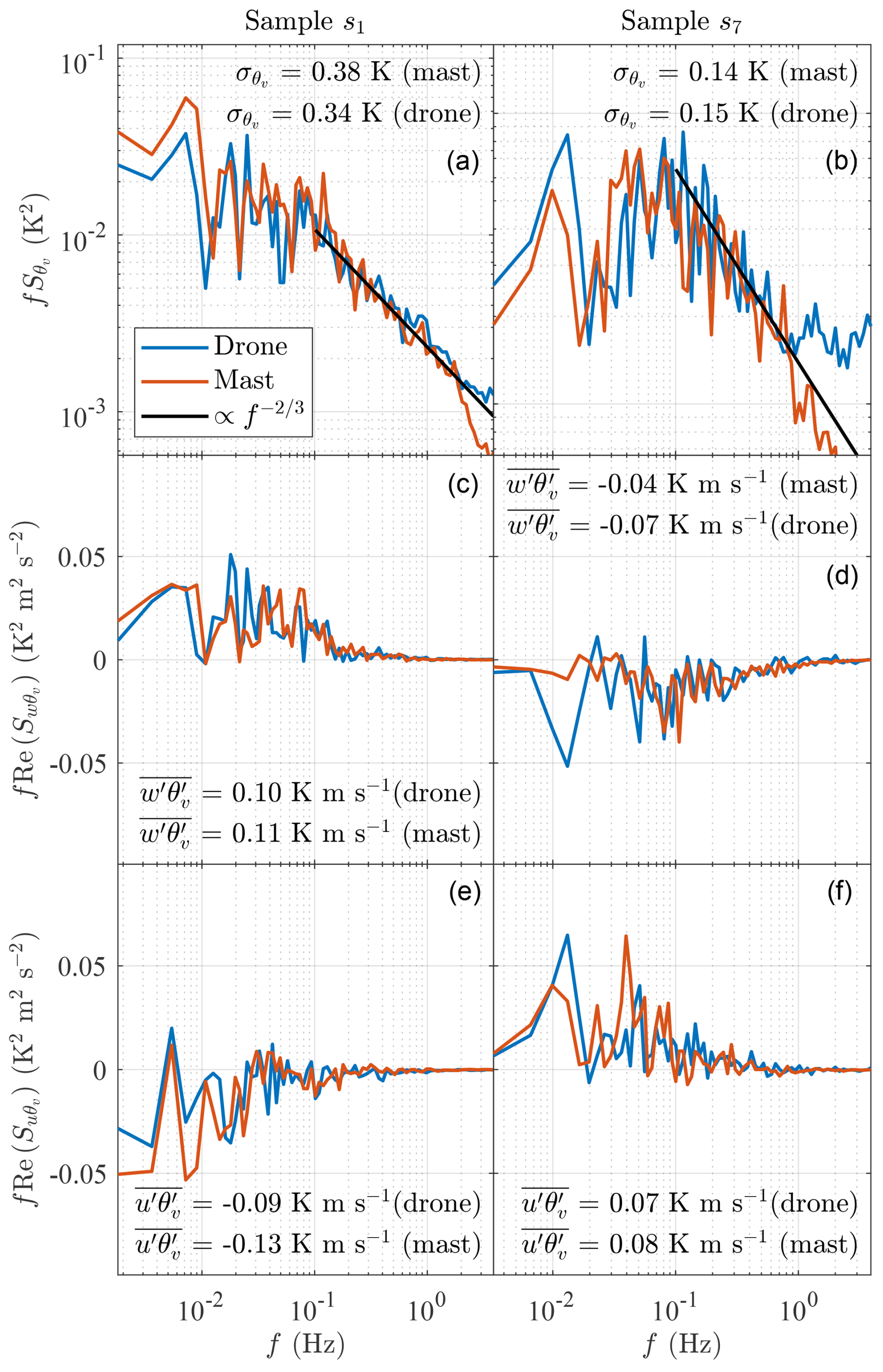
Figure 11 PSD estimates of the sonic temperature (θ_v) and associated CPSDs, including the vertical ($Re\left(S_{w{\mathit{\theta }}_v}\right)$) and along-wind ($Re\left(S_{u{\mathit{\theta }}_v}\right)$) components for both the flying sonic anemometer (blue line) and the one mounted on the mast (orange line) 30 m above the ground for samples s₁ (a, c, e) and at 60 m above the ground for samples s₇ (b, d, f).

Notably, the PSD for sample s₁ demonstrates an excellent agreement between the sonic temperature from the mast-mounted sensor and SAMURAI-S. However, for sample s₇, the PSD of the drone-based anemometer deviates from the expected $-\mathrm{5}/\mathrm{3}$ power law at frequencies greater than 1 Hz. This deviation scales with frequency f, suggesting the influence of white noise on the measurement data. For the mast-mounted anemometer, the PSD estimates of the temperature exhibit slight discrepancies from this $-\mathrm{5}/\mathrm{3}$ power law in samples s₁ and s₇. Additional plots showing PSD spectra for samples s₅, s₆, s₈, s₉, and s₁₀ are provided in Appendix B.

5.2 Mean and turbulence statistics comparison

This section presents a detailed analysis of the sensor performance, focusing on integral mean flow and turbulence characteristics for all three velocity components u, v, and w (Figs. 12 and 13).

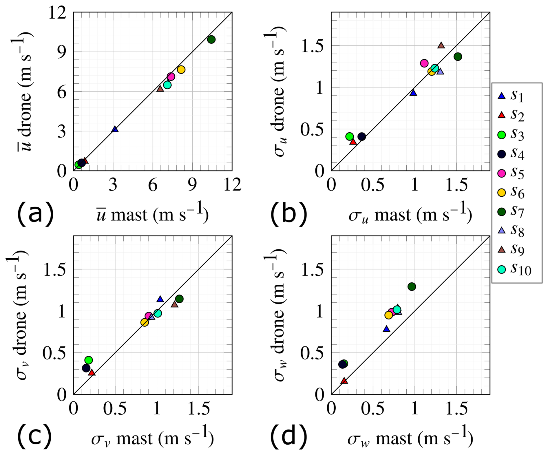
Figure 12 Mean wind speed and standard deviation of the three velocity components for the mast- and the drone-mounted sonic anemometers across the 10 validation samples. Circle markers indicate measurements from the mast at 30 m above the surface, while triangle markers correspond to measurements at 60 m.

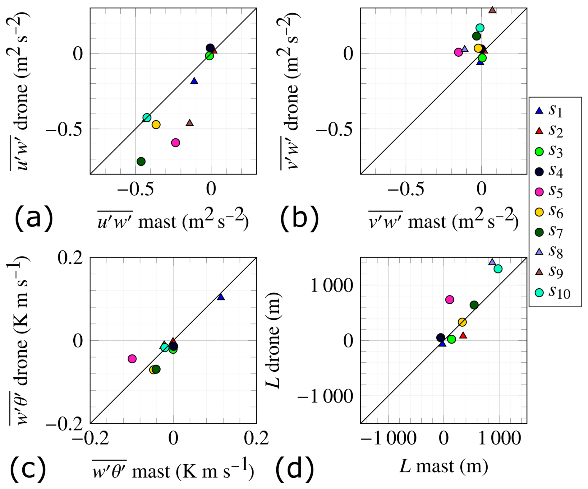
Figure 13 Turbulence covariance and Obukhov length for the 10 validation samples, as measured by the mast- and the drone-mounted sonic anemometers. Circle markers represent measurements from the mast at 30 m above the surface, whereas triangle markers signify measurements at 60 m.

The drone-mounted anemometer slightly underestimates the mean wind speed $\stackrel{\mathrm{‾}}{u}$ (Fig. 12a), but the data scatter is low. The height difference between the two sensors may explain this underestimation (Table 4). More specifically, the payload heights were on average 4 and 8.5 m lower than the target altitudes for the sonic sensor at 30 and 60 m, respectively. The standard deviations of the along-wind and across-wind velocity components denoted σ_u (Fig. 12b) and σ_v (Fig. 12c), respectively, show excellent agreement. The drone-mounted anemometer slightly overestimates the standard deviation σ_w of the vertical component (Fig. 12d), and this overestimation increases nearly linearly with the mean wind speed in absolute terms.

The covariance estimates $\stackrel{\mathrm{‾}}{u^{\prime }{w}^{\prime }}$ (Fig. 13a) exhibit a larger scatter than $\stackrel{\mathrm{‾}}{v^{\prime }{w}^{\prime }}$ (Fig. 13b). At the same time, the covariance estimate of $\stackrel{\mathrm{‾}}{{\mathit{\theta }}^{\prime }{w}^{\prime }}$ (Fig. 13c) and the Obukhov length L (Fig. 13d) demonstrate good correlation and small scatter. The vertical velocity component is used in the numerator and denominator when calculating L. Thus, the lower scatter may be attributed to the larger uncertainties associated with component w cancelling each other to some degree. Sample s₅, depicted in pink, consistently exhibits the highest scatter. This sample has the shortest duration, lasting only 10 min, which is at least 4.7 min shorter than all other samples. Thus, sample s₅ may be more prone to errors associated with insufficient sampling of the largest turbulent eddies.

Figure 14 compares the integral length scales for each velocity component, estimated following the procedure presented in Fig. 4.3. Samples s₂, s₃, and s₄ did not satisfy the conditions required to apply Taylor's hypothesis of frozen turbulence, which were defined as a turbulence intensity of $I_u={\mathit{\sigma }}_u/\stackrel{\mathrm{‾}}{u}<\mathrm{0.5}$ and a mean wind speed of $\stackrel{\mathrm{‾}}{u}>$ 1 ms⁻¹. All other samples met these conditions, with I_u ranging from 0.15 to 0.31 and a mean wind speed exceeding 3 ms⁻¹.

The streamwise length scale L_u (Fig. 14, left panel) shows a rather large scatter around the 1:1 line. However, there is no systematic deviation between mast and drone measurements. In contrast, the middle panel suggests that the drone-mounted anemometer systematically underestimates the lateral length scale L_v. However, it is unclear whether this discrepancy arises from sensor characteristics or the specific position of the drone. The best agreement is observed in the right panel for the vertical length scale L_w, which exhibits low scatter and no clear bias, despite the overestimation of σ_w by the drone-mounted sonic anemometer (Fig. 12d).

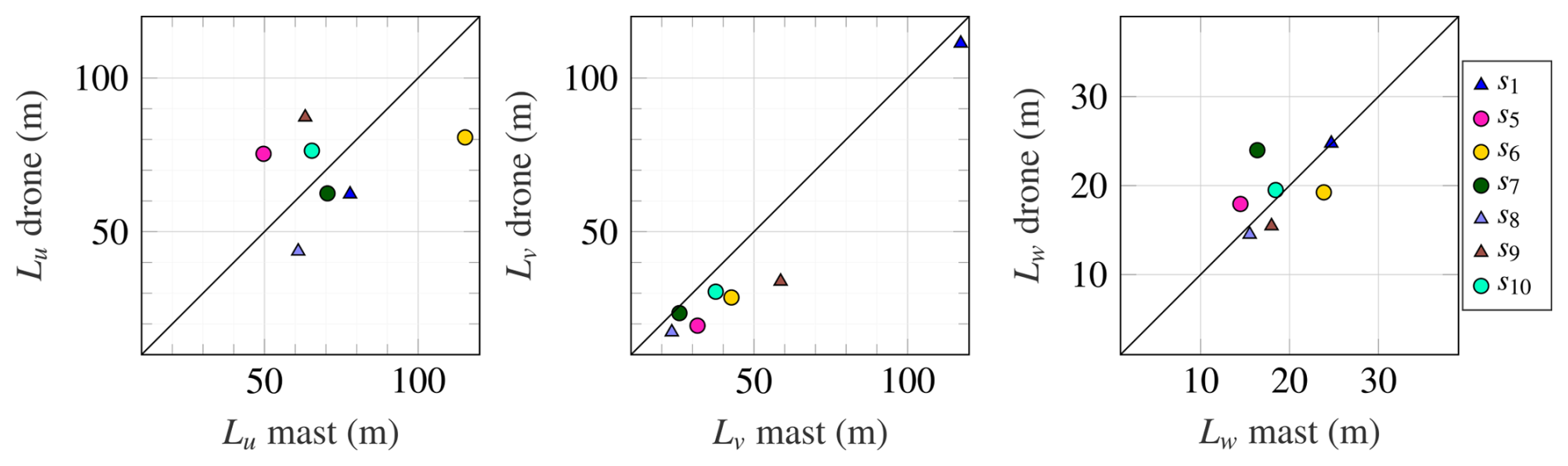
Figure 14 Integral turbulence length scale of the three velocity components for the mast- and the drone-mounted sonic anemometers across the 10 validation samples. Circle markers indicate measurements from the mast at 30 m above the surface, while triangle markers correspond to measurements at 60 m. Only samples associated with I_u<0.5 and $\stackrel{\mathrm{‾}}{u}>\mathrm{1}$ ms⁻¹ are used to satisfy the conditions required for applying Taylor's hypothesis of frozen turbulence.

The discrepancies between the vertical velocity spectral densities estimated by the mast-mounted sonic anemometers and by the drone are explored in more detail through the ratios $S_w/S_u$ and $S_v/S_u$, following the method presented in Sect. 4.1. Chamecki and Dias (2004) states that if the spectral ratio trends towards 4/3 without actually reaching it, this could indicate that isotropy in the inertial subrange has not been achieved within the examined frequency range, a situation typically occurring under stable atmospheric conditions. In this study, the spectral ratios reached a plateau for all 10 samples, albeit not always with a value of 4/3. This suggests that the atmospheric conditions were favourable for observing local isotropy but that flow distortion may have been present. The results for all the samples are shown in Fig. 15. Values corresponding to s₂, s₃, and s₄ are displayed with grey triangle markers to highlight their non-stationary nature, which does not fit within the analysis framework. The following discussion and comments exclude these three samples unless explicitly stated otherwise.

Figure 15 shows that only one sample from the drone-based dataset is close to the theoretical ratio of 1.33 for $<S_w/S_u>$. As wind speed increases, the ratio measured by SAMURAI-S diverges further from 1.33, whereas the mast data fluctuate between 1.0 and 1.25. This could be related to the larger σ_w values measured by the drone setup.

Although the mast data appear closer to the expected ratio of 1.33 compared to the SAMURAI-S, they could still represent an underestimation of up to 20 % of the vertical fluctuating component. As discussed above, not achieving the $\mathrm{4}/\mathrm{3}$ ratio may hint at the presence of flow distortion caused by the mast or the sonic anemometer itself, contributing to this underestimation.

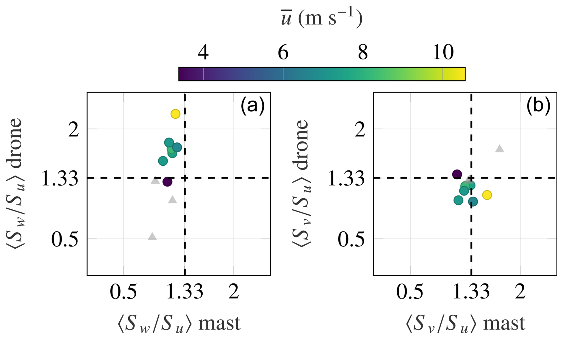
Figure 15 Quadrant analysis for the frequency-averaged spectral ratios $<S_w/S_u>$ (a) and $<S_v/S_u>$ (b) with fr>2 and fr<10 between the mast- and drone-based measurements for different mean wind speeds. The notation $<>$ denotes an average over frequency bins. Samples with a mean wind speed below 1 ms⁻¹ are marked as grey triangles, as they are representative of intermittent turbulence, for which the assumption of local isotropy in the inertial subrange may not be defined.

Figure 16 Uncertainty metrics (Eqs. 10 to 13) estimated for the drone-mounted sensor (y axis) and the mast-mounted sensor (x axis). The green patch represents the region with low statistical uncertainties.

Similar observations apply for the ratio $<S_v/S_u>$. For $\stackrel{\mathrm{‾}}{u}>\mathrm{6}$ ms⁻¹, the ratio $<S_w/S_u>$ exceeds the expected value of 1.33 in drone measurements.

The data recorded in this study mainly represent stable or near-neutral atmospheric conditions. An exception is found in s₁, collected under unstable atmospheric conditions ($\mathit{\zeta }=-\mathrm{0.46}$), and shows one of the closest agreements between the drone and mast-mounted sensors. It should also be noted that for all flights except s₁ the wind consistently came from the 280 to 310 ° sector. The limited number of samples and the variability in stability and wind direction prevent determining whether the improved agreement under unstable conditions is a systematic effect or influenced by differences in wind direction over heterogeneous topography. Further research is necessary to determine whether convective conditions consistently enhance the performance of the drone-based setup described in this paper.

5.3 Uncertainties analysis

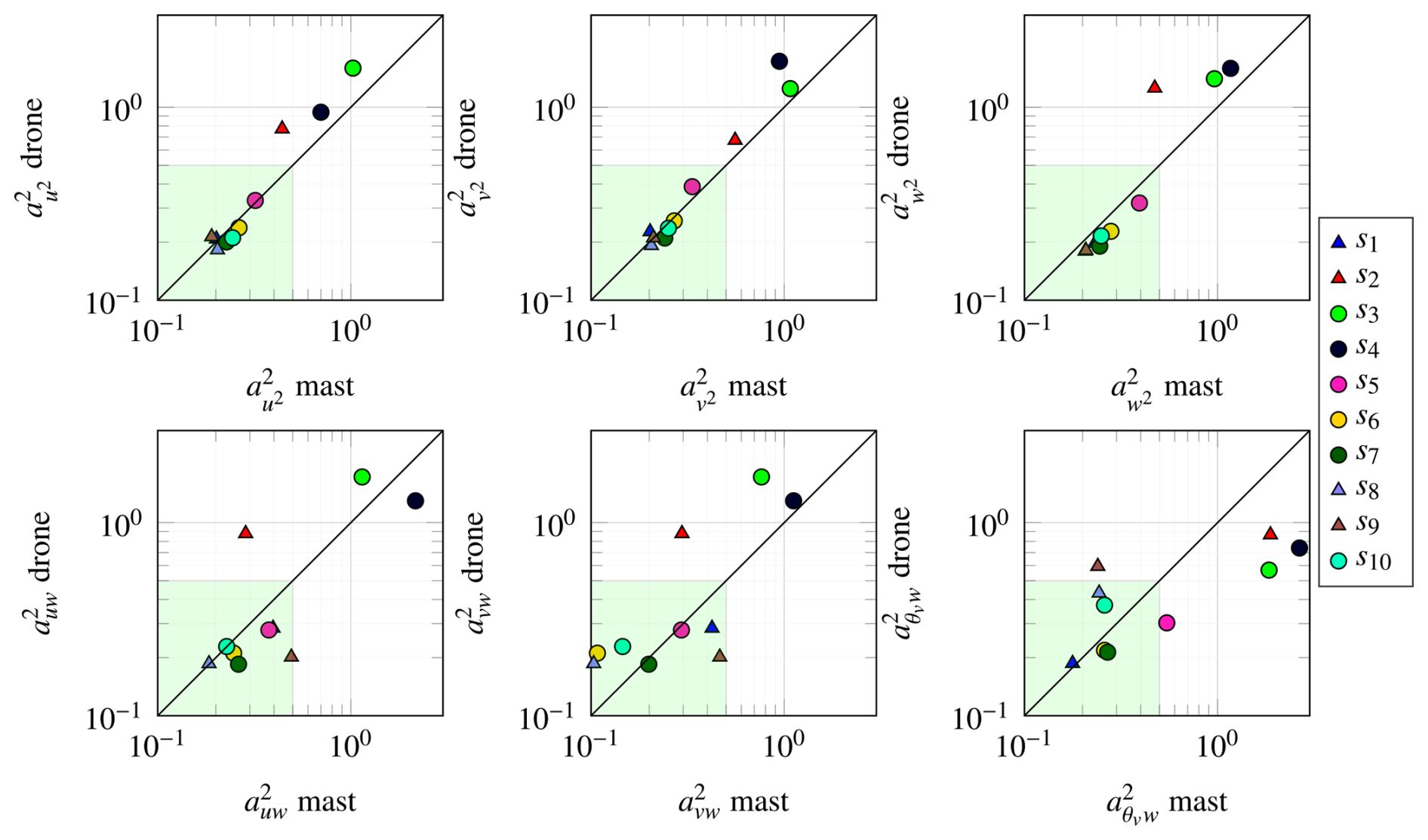
Figure 16 presents the uncertainty metrics associated with the calculation of ${\mathit{\sigma }}_u^{\mathrm{2}}$, ${\mathit{\sigma }}_v^{\mathrm{2}}$, ${\mathit{\sigma }}_w^{\mathrm{2}}$, $\stackrel{\mathrm{‾}}{u^{\prime }{w}^{\prime }}$, $\stackrel{\mathrm{‾}}{v^{\prime }{w}^{\prime }}$, and $\stackrel{\mathrm{‾}}{{\mathit{\theta }}_v^{\prime }{w}^{\prime }}$. Most samples exhibit reasonably low uncertainties, as indicated by the green patch in Fig. 16, which corresponds to a normalized value of 0.5, consistent with that used in Stiperski and Rotach (2016) and Cheynet et al. (2019). However, samples s₂, s₃, and s₄ systematically fall outside this green area due to the low wind speed at the time of recording. Consequently, they should not be included in the analysis of turbulence statistics, at least within the framework of stationary homogeneous turbulence. These samples exhibit characteristics of intermittent turbulence, the study of which is beyond the scope of this work.

In Fig. 16, the uncertainty metric $a_{{\mathit{\theta }}_{v}w}^{\mathrm{2}}$ shows higher-than-expected uncertainties for samples s₅ and s₉. The relatively high uncertainty for sample s₅ is partly attributable to the short duration of the record – around 10 min, which results in large uncertainties for covariance estimates. Sample s₉ has a record duration of approximately 17 min, so the high uncertainty value remains unclear, notably since it is only visible in the covariance between the sonic temperature and the vertical velocity component of the drone-mounted anemometer. It should be noted that the uncertainty metrics are generally comparable between the drone-based and mast-based measurements, supporting the potential of this mobile platform for turbulence analysis.

6 Conclusions

This study presents a pioneering effort in atmospheric research, focusing on using a research-grade 3D sonic anemometer mounted 18 m under a drone to observe turbulence. The goal was to assess the effectiveness of drone-mounted sonic anemometers as a versatile tool for turbulence measurement, challenging traditional methods that mount the same sensor on masts or towers. A notable aspect of this research was the application of a dynamic motion compensation algorithm that accounts for the motion and tilt of the sonic anemometer. At the same time, the drone hovered above the location of interest.

Data collection took place during the Models and Observations for Surface Atmosphere Interactions (MOSAI) campaign in France. The methodology included a comparative analysis between conventional mast-mounted 3D sonic anemometers at 30 and 60 m above ground and the drone-mounted anemometer. This comparison focused on mean flow and turbulence statistics, including the integral length scales, covariance, and auto-power and cross-power spectral densities of velocity fluctuations. Our findings indicate that the drone-mounted anemometer effectively captures detailed turbulence measurements. Although there is good agreement regarding the along-wind and across-wind flow when comparing the drone and mast data, drone-based observations consistently overestimate vertical wind fluctuations across all flights. This overestimation increases as the wind speed increases, calling for further analysis under a broader range of wind conditions. Also, our findings show that the drone-mounted sensor and mast-mounted sonic anemometers provide turbulence statistics with similar levels of uncertainty.

For the drone-mounted anemometer, the spectral ratio $S_w/S_u$ was up to 63 % larger than the local isotropy hypothesis predicted in the inertial subrange. However, it was also observed that the mast-mounted anemometer could significantly underestimate the vertical turbulence component, with a spectral ratio $S_w/S_u$ that was up to 22 % lower than predicted by the local isotropy hypothesis in the inertial subrange.

The sonic temperature and the Obukhov length estimated by both sensors were also investigated. The comparison provides a positive and encouraging overall picture, with good agreement between the mast and drone measurements. The only exception is the shortest duration sample (10 min compared to at least 15 min for all others), which exhibits markedly divergent behaviour compared to its mast-measured counterpart.

Overall, the findings underscore the potential of the SAMURAI-S system, especially its complementarity with mast-mounted sonic anemometers and scanning Doppler wind lidar for studying three-dimensional turbulence in the atmosphere.

Appendix A: Transformation matrix

The transformation matrix $\mathbf{R}(\mathit{\varphi },\mathit{\theta },\mathit{\psi })$ is defined as

$$\mathbf{R}(\mathit{\varphi },\mathit{\theta },\mathit{\psi })=\left[{\mathbf{R}}_{\mathrm{3}}\right(\mathit{\varphi }\left){\mathbf{R}}_{\mathrm{2}}\right(\mathit{\theta }\left){\mathbf{R}}_{\mathrm{1}}\right(\mathit{\psi }){]}^{\text{T}}$$

where

$${\displaystyle }{\mathbf{R}}_{\mathrm{1}}\left(\mathit{\psi }\right){\displaystyle }=\left(\begin{array}{ccc}\cos \mathit{\psi }& \sin \mathit{\psi }& \mathrm{0}\\ -\sin \mathit{\psi }& \cos \mathit{\psi }& \mathrm{0}\\ \mathrm{0}& \mathrm{0}& \mathrm{1}\end{array}\right),$$

$${\displaystyle }{\mathbf{R}}_{\mathrm{2}}\left(\mathit{\theta }\right){\displaystyle }=\left(\begin{array}{ccc}\cos \mathit{\theta }& \mathrm{0}& -\sin \mathit{\theta }\\ \mathrm{0}& \mathrm{1}& \mathrm{0}\\ \sin \mathit{\theta }& \mathrm{0}& \cos \mathit{\theta }\end{array}\right),$$

$${\displaystyle }{\mathbf{R}}_{\mathrm{3}}\left(\mathit{\varphi }\right){\displaystyle }=\left(\begin{array}{ccc}\mathrm{1}& \mathrm{0}& \mathrm{0}\\ \mathrm{0}& \cos \mathit{\varphi }& \sin \mathit{\varphi }\\ \mathrm{0}& -\sin \mathit{\varphi }& \cos \mathit{\varphi }\end{array}\right).$$

Appendix B: Power spectral density estimates for other samples

Figure B1 presents the power spectral densities of the three velocity components, as well as the cross-spectral densities between u and w, for samples s₅, s₆, s₈, s₉, and s₁₀, where the concept of spectral density is well-defined. For clarity, these spectral densities are normalized by the variance or covariance of the corresponding variable. Similarly, Fig. B2 displays the normalized power spectral densities of the sonic temperature, along with the normalized co-spectral densities. These figures exhibit trends similar to those observed for samples s₁ and s₇, which were analysed in detail in this study.

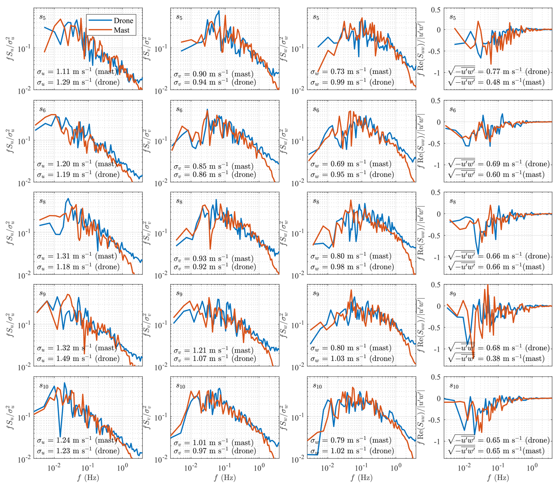
Figure B1 Normalized power spectral densities of the three velocity components and co-spectral densities for samples s₅, s₆, s₈, s₉, and s₁₀.

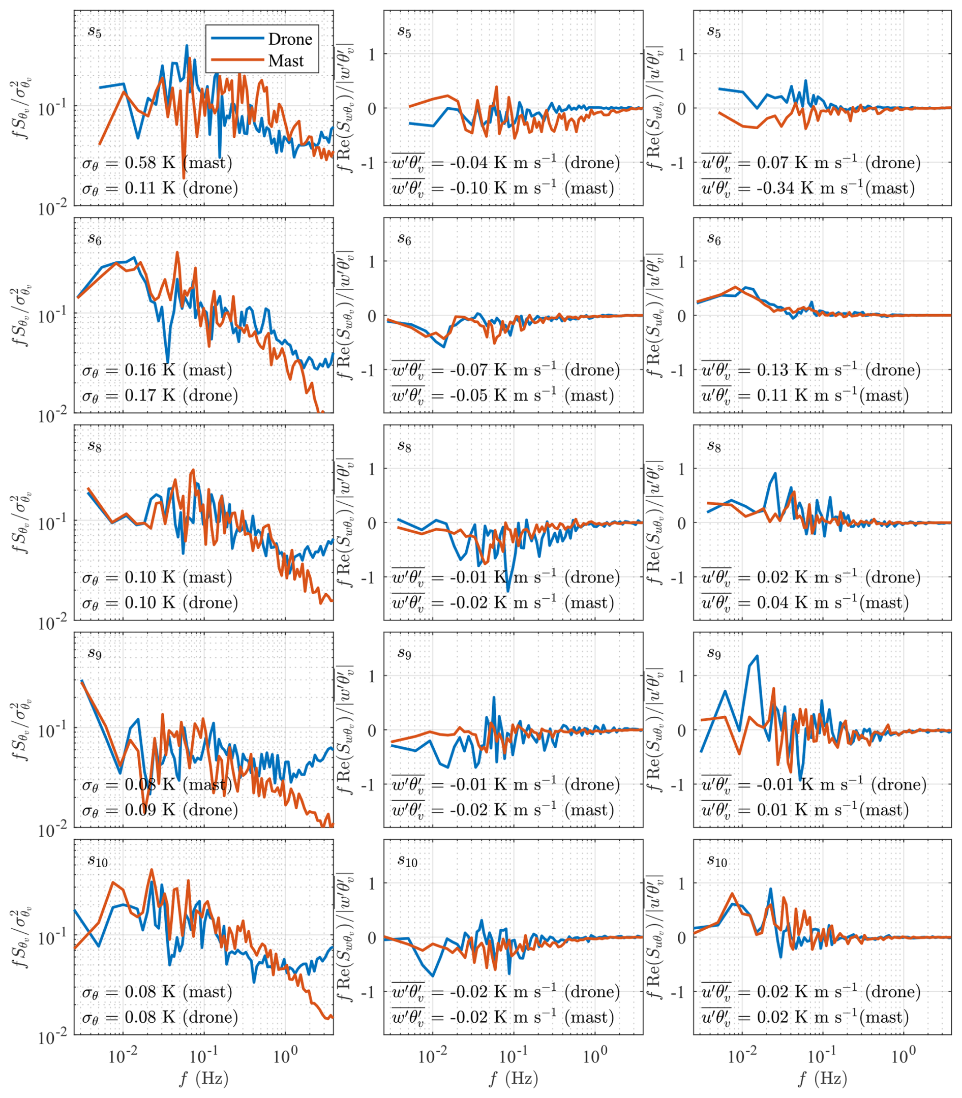
Figure B2 Normalized power spectral densities of the sonic temperature and associated co-spectral densities for samples s₅, s₆, s₈, s₉, and s₁₀.