An introduction of the Three-Dimensional Precipitation Particle Imager (3D-PPI)

The Three-Dimensional Precipitation Particle Imager (3D-PPI) is presented as a new instrument for measuring the size, fall velocity, and three-dimensional shape of precipitation particles. The 3D-PPI consists of three high-resolution cameras with telecentric lenses and one high-speed camera with one non-telecentric lens. The former captures high-resolution images of falling particles from three angles, enabling three-dimensional (3D) shape reconstruction via a 3D reconstruction algorithm, while the large observation volume facilitates particle size distribution (PSD) analysis. The latter records the images of the falling precipitation particles with 200 frames per second, based on which the falling velocity of particles can be calculated. The field experiment of the 3D-PPI and OTT Parsivel disdrometer (OTT) was conducted in Tulihe, China, with more than 880 000 snowflakes recorded during a typical snowfall case lasting 13 h, and the results indicate strong agreement between the PSDs obtained by the 3D-PPI and those obtained by the OTT. This demonstrates its potential application in atmospheric science, polar research, and other fields.

1 Introduction

Precipitation microphysics refers to the interactions and processes associated with the scale of individual precipitation particles. Microphysics and microstructure, i.e., the distribution of particle properties, such as size, shape, density, and mass, together determine the state and evolution of clouds and precipitation at this scale and are intrinsic to the process of cloud and precipitation evolution (Taylor, 1998). The microphysical properties of spherical (or ellipsoidal) raindrops are relatively well studied. Research on ice-phase precipitation (such as snowflakes) microphysics is complicated by the complex geometry of individual snowflakes. Minor variations in air temperature and humidity can cause significant changes in the shape of ice crystals, resulting in a wide variety of crystal shapes ranging from simple plates and columns to complex dendrites or needles (Bailey and Hallett, 2012). Aggregation combines individual crystals into complex and random shapes of snowflakes. Despite the challenges associated with measuring snowflake shapes, the significance of this work is substantial. Accurate measurement of snowflake shapes is crucial for advancing our understanding of atmospheric sciences, particularly in ice- and mixed-phase cloud formation and precipitation processes (Morrison et al., 2020). Specifically, accurate descriptions of snowflake shapes are critical for triple-frequency radar retrievals, as they directly influence the interpretation of radar echoes and the assessment of snow's microphysical properties (Mason et al., 2019). Moreover, precise shape descriptions of snowflakes will significantly improve radar-based quantitative winter precipitation estimation (Notaroš et al., 2016).

The absence of accurate information on the three-dimensional (3D) shape of precipitation particles leads to errors in the parameterization of physical processes in cloud precipitation and quantitative precipitation estimation (QPE) using weather radar. The assumption that true snowflakes are ellipsoidal may lead to inaccurate scattering matrix calculations and hence incorrect determinations of snow water equivalent (Tyynelä et al., 2011). The ellipsoid approximation is valid only for smaller particles. As snowflake size increases, shape properties become increasingly significant in scattering calculations (Olson et al., 2016). Between isovolumetric spheres and hexagonal columns, more accurate snowflake models are needed. In addition, an assessment of the sensitivity of high-frequency falling-snow characteristics using an idealized simulated snowflake model indicates the necessity for a scattering database of snowflakes, in which three highly variable shapes should be taken into consideration (Kneifel et al., 2010). Ideal ice crystal models were created in dendritic, thin plate, stellar plate, crown prism, and hollow column forms, and the scattering effects of these geometries were calculated using the discrete dipole approximation (DDA) approach (Kim, 2006). The results indicate that the scattering characteristics of these ideal snowflakes are highly sensitive to their shapes. This further emphasizes the necessity for accurate shape modeling (Kim et al., 2007).

Various in situ instruments have been developed to measure precipitation particles. The OTT Parsivel disdrometer measures the size and fall velocity of particles based on laser signal attenuation and duration (Loffler-Mang and Joss, 2000). However, the 1D measurement concept requires additional assumptions to correctly size irregularly shaped particles such as snowflakes (Battaglia et al., 2010), and the shape of particles cannot be obtained. The Two-Dimensional Video Disdrometer (2DVD) can obtain the 3D particle shape by using two line-scan cameras with an angle of 90°, where the sampling area is 10 × 10 cm² (Bernauer et al., 2016). Particle shape estimates may still be biased due to horizontal winds (Helms et al., 2022). The Multi-angle Snowflake Imager (MSI) can obtain the 3D shape and fall velocity of individual snowflakes by using four line-scan cameras with an angle of 45°; however, a limitation lies in its restricted sampling area, allowing for the measurement of only one snowflake within a narrow field of view (Minda et al., 2017).

In addition to line-scan cameras, several planar camera instruments have been developed. The Snowfall Video Imager (SVI) employs a camera and a light source to record the images of snowflakes in free fall. Its subsequent evolution, the Precipitation Imaging Package (PIP), employs advanced digital image processing algorithms to enhance the precision and resolution of snowflake imaging (Newman et al., 2009; Pettersen et al., 2020). The PIP provides physically consistent estimates of snowfall intensity and volume-equivalent densities from high-speed images, although its equivalent-density parameterization requires further refinement for extremely high snow-to-liquid ratio snowfall events (Pettersen et al., 2020). The Video Precipitation Sensor (VPS) can obtain the shape and fall velocity of hydrometeors when the particles fall through the sampling volume. The camera is exposed twice in a single frame, which allows for the double exposure of particle images to be recorded, and the size and fall velocity of particles can be obtained simultaneously (Liu et al., 2014, 2019). The Video In Situ Snowfall Sensor (VISSS) consists of two cameras with LED backlights and telecentric lenses and can measure the shape and size of snowflakes in a large observation volume with high pixel resolution (43 to 59 µm px⁻¹) (Maahn et al., 2024). Nevertheless, it is challenging to resolve highly fine structures of snowflakes with only two angles of observation.

The Multi-Angle Snowflake Camera (MASC) simultaneously captures three high-resolution images of falling hydrometeors from three different viewpoints (Garrett et al., 2012), which provides the conceptual possibility of 3D reconstruction of the observed snowflakes. The visual hull (VH) algorithm was used to reconstruct the 3D shape of snowflakes through multi-angle imaging, and the addition of two more cameras to MASC has been shown to improve reconstruction results (Kleinkort et al., 2017). Incorporating the rich dataset from MASC, the 3D-GAN model is adeptly trained to reconstruct the intricate 3D architecture of snowflakes, thereby unlocking new dimensions in the study of snowfall microphysics (Leinonen et al., 2021). Furthermore, MASCDB is a comprehensive database of images, descriptors, and microphysical properties of individual snowflakes in free fall and showcases the MASC's exceptional potential for contributing to the field of atmospheric science by providing an extensive and detailed resource for studying the microphysical properties of snowflakes (Grazioli et al., 2022).

Currently, instruments are needed that not only provide a finer 3D structure of snowflakes but also capture enough particles per unit of time to estimate the particle size distribution (PSD). This study presents a new instrument: the Three-Dimensional Precipitation Particle Imager (3D-PPI). The instrument's design and main components are introduced in Sect. 2; the calibration of the cameras is described in Sect. 3; and detailed algorithms, including image processing, particle matching, particle localization, and 3D reconstruction, are presented in Sect. 4. The preliminary results of the field experiment are discussed in Sect. 5, and the last part summarizes the main results and future work of the 3D-PPI.

2 Instrument design

The 3D-PPI contains three identical high-resolution cameras with telecentric lenses (numbered Cam0, Cam1, and Cam2 in this paper) and one high-speed camera with a non-telecentric lens (numbered Cam3). Four high-brightness LED arrays are used as light sources to illuminate the observation volume. Additionally, a ZYNQ driver circuit has been developed to control the cameras and light source and to transmit the raw images to the PC terminal. To improve the instrument's working efficiency, a capacitive rain sensor is adopted as a trigger, meaning the cameras only work when precipitation occurs. The sensor detects any moisture on the instrument's surface, and its heating element ensures that snow is melted and appropriately sensed. To mitigate the effects of wind on camera alignment, we designed the 3D-PPI with a protective cover that effectively shields the cameras from wind disturbances. The concept illustration and prototype, as well as snowflake images of the 3D-PPI, are shown in Fig. 1.

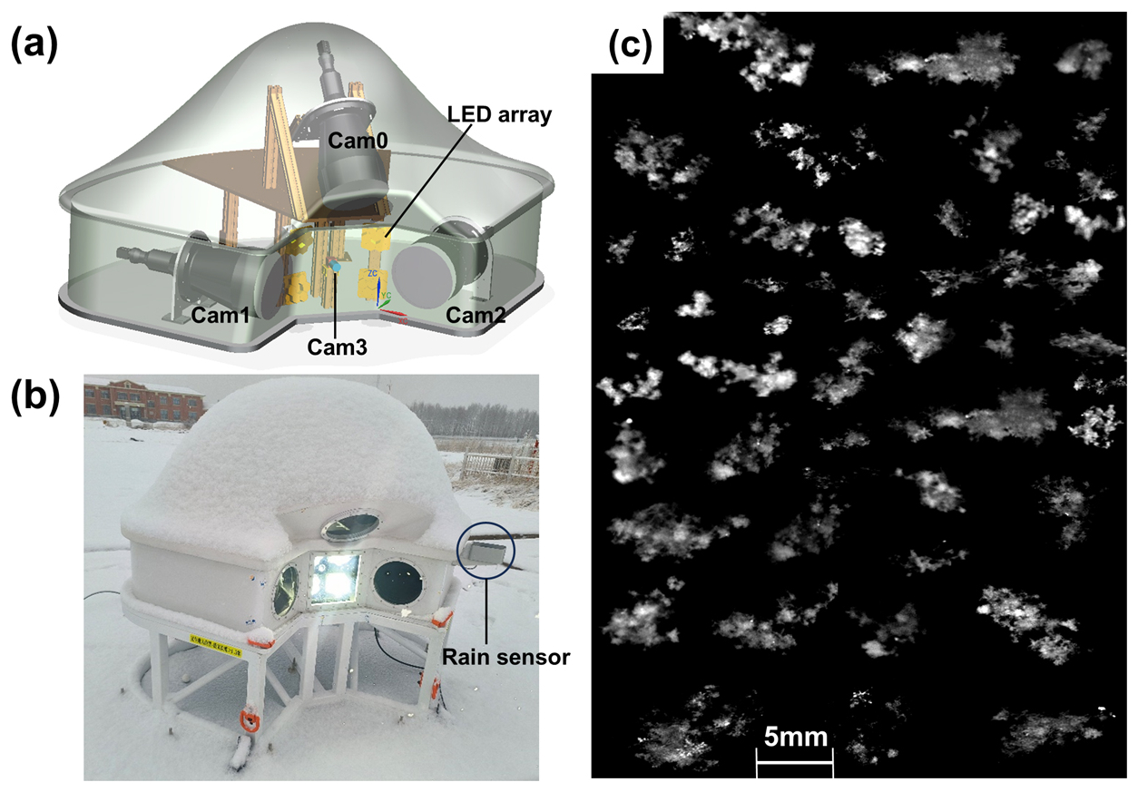
Figure 1 (a) Concept illustration of the 3D-PPI. (b) The prototype of the 3D-PPI deployed at Tulihe, China. (c) Randomly selected snowflakes were observed on 6 April 2024 between 04:53 and 11:13 UTC.

The high-speed camera is positioned horizontally at the center, Cam1 and Cam2 are positioned at 45° on either side of the high-speed camera in the same horizontal plane, and Cam0 is positioned at 45° vertically above (Fig. 1a). The high-brightness LED array light sources are situated on the same side as the cameras to illuminate the observation volume. The four cameras, lenses, and LED lights, including the additional beams of the 3D-PPI, are illustrated in Fig. 2. To clarify, the observation volume (OV) of one high-resolution camera is a cuboid defined by the following three dimensions: a, b, and d (170, 125, and 88 mm), which represent the length, width, and depth of the field of view, respectively. The intersection of the three OVs of the three high-resolution cameras forms the effective OV of the 3D-PPI (775 cm³). Only the particles falling within the effective OV of the 3D-PPI can be simultaneously captured by the three high-resolution cameras, and their 3D shapes can then be reconstructed three-dimensionally.

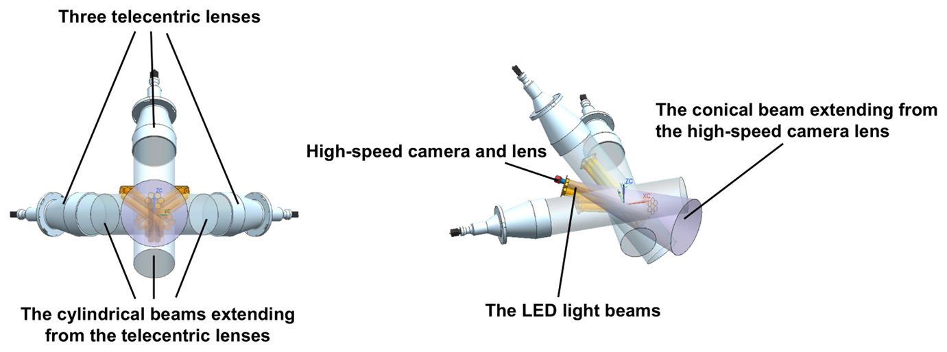
Figure 2 Two views of four cameras and lenses, including additional beams extending from the lenses and the LED light beams.

The high-resolution camera is a Sony IMX304 with a resolution of 4096 × 3000 grayscale pixels and a frame rate of 5 fps. The high-speed camera is a Sony IMX287 with a resolution of 720 × 540 grayscale pixels and a frame rate of 200 fps. The detailed technical parameters are shown in Table 1 and are divided into two parts, the image sensor and the lens.

Table 1 Technical specifications of the cameras.

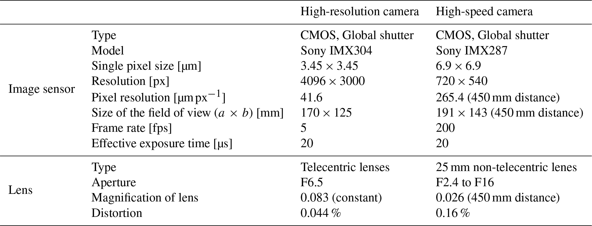
For the high-resolution camera, the single pixel size is 3.45 µm, and the magnification of the lens is 0.083, meaning that the pixel resolution is 41.6 µm px⁻¹. Telecentric lens distortion is 0.044 % and can be ignored. For the high-speed camera, the single pixel size is 3.45 µm, and the magnification is 0.026 at a working distance of 450 mm, meaning that the pixel resolution is 265.4 µm px⁻¹.

The utilization of telecentric lenses eliminates the sizing error caused by the uncertain distance between the snowflakes and the cameras. Unlike non-telecentric lenses, which produce larger images of nearby objects and smaller images of distant objects (Fig. 3a), telecentric lenses are based on the principle of parallel-light imaging, resulting in identical objects at different distances from the lens having the same size in the image (Fig. 3c). This difference in imaging characteristics will lead to distinct methods for 3D reconstruction (Fig. 3b, d), which are discussed in detail in Sect. 4. With an optical distortion of 0.044 %, the telecentric lens effectively minimizes distortion, establishing a linear correspondence between image coordinates and world coordinates. This alignment greatly simplifies camera calibration, as elaborated upon in Sect. 3.

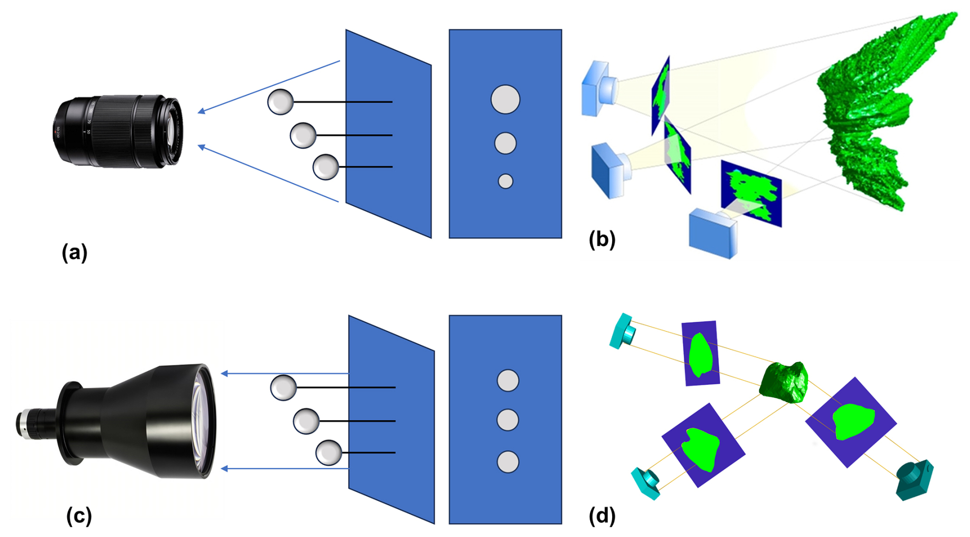
Figure 3 Illustration of imaging characteristics and reconstruction of a snowflake using three cameras. (a) Non-telecentric lens imaging characteristics, (b) non-telecentric lenses back-projected to obtain three visual cones (Kleinkort et al., 2017), (c) telecentric lens imaging characteristics, and (d) telecentric lenses back-projected to obtain three visual columns.

The 3D-PPI has four light source arrays, each consisting of six high-brightness LEDs organized into a cluster to create an array lighting system. Each LED is 5 W with a total power of 120 W. This LED lighting system integrates a high-brightness LED chip, substrate, heat sink, casing, leads, protective features, and other functionalities into a single unit. At its core lies the LED chip, utilizing white high-brightness LED chips. Each LED is equipped with a converging lens, facilitating the creation of a cone-shaped beam of light. Once triggered, the LEDs will continue to illuminate, providing consistent lighting throughout the exposure period. The design and physical representation of the LED array lighting system are illustrated in Fig. 4. The LED light sources are configured in parallel, allowing for a single power supply connection that distributes power to the entire array. Each LED can operate in either constant-current mode or trigger mode. In constant-current mode, the LEDs provide stable and uniform light intensity, which enhances the uniformity of illumination within the OVs.

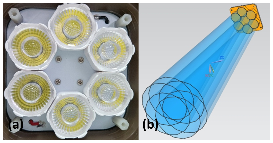
Figure 4 (a) LED array lighting group design. (b) Cone-shaped beam formed by LED array lighting group.

3 Calibration of cameras

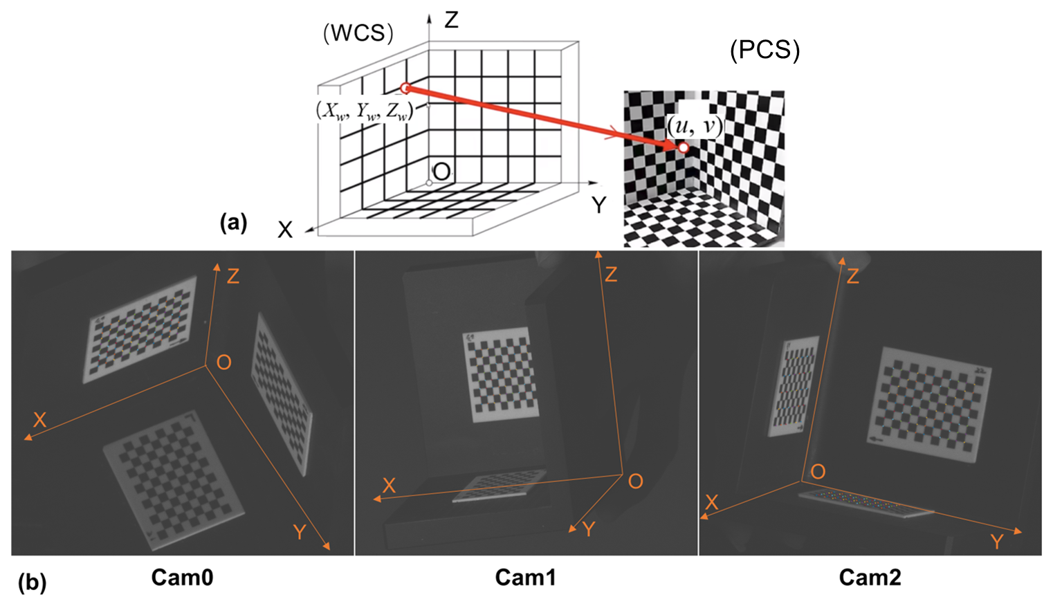
Camera calibration is the basis for obtaining 3D spatial information from 2D images. There is a one-to-one correspondence between the spatial scene points and their image points in the image, and their positional relationship is determined by the camera imaging geometric model (Cheng and Huang, 2023). The parameters of this geometric model are called camera parameters, which can be determined by an experiment and computation, and the process of solving the parameters experimentally and computationally is called camera calibration. The geometric model for telecentric lens imaging is described in detail in Appendix A, where four coordinate systems (the world coordinate system (WCS), camera coordinate system (CCS), image coordinate system (ICS), and pixel coordinate system (PCS)) are defined and their transformations derived. The purpose of camera calibration in this section is to estimate the projection matrices KM₀, KM₁, and KM₂ for the three high-resolution cameras (Cam0, Cam1, and Cam2, respectively), which enables the transformation of 3D spatial points in the WCS to their corresponding pixel coordinates on the image plane in PCS. Appendix A derives a model that assumes linear, telecentric imaging without distortion. Based on this model, Eq. (A6) is transformed to

$$\begin{array}{}\text{(1)}& \left[\begin{array}{cccc}\frac{\mathit{\beta }}{S_{\mathit{\nu }}}{r}_{\mathrm{11}}& \frac{\mathit{\beta }}{S_{\mathit{\nu }}}{r}_{\mathrm{12}}& \frac{\mathit{\beta }}{S_u}{r}_{\mathrm{13}}& \frac{\mathit{\beta }}{S_u}{t}_x+u_{\mathrm{0}}\\ \frac{\mathit{\beta }}{S_{\mathit{\nu }}}{r}_{\mathrm{21}}& \frac{\mathit{\beta }}{S_{\mathit{\nu }}}{r}_{\mathrm{22}}& \frac{\mathit{\beta }}{S_{\mathit{\nu }}}{r}_{\mathrm{23}}& \frac{\mathit{\beta }}{S_u}{t}_y+{\mathit{\nu }}_{\mathrm{0}}\end{array}\right]\left[\begin{array}{c}{X}_w\\ Y_w\\ Z_w\\ \mathrm{1}\end{array}\right]=\left[\begin{array}{c}u\\ \mathit{\nu }\end{array}\right],\end{array}$$

where β is the telecentric camera magnification; S_u and S_v are the length and width dimensions of the individual image; r_ij and t_x(t_y) denote the matrix elements of the rotation and translation process from the WCS to the CCS, respectively, and these parameters relate solely to the relative position of the cameras; and u₀ and v₀ are the horizontal and vertical coordinates of the camera's main point offsets, which may change over time.

The coordinate points (X_w, Y_w, Z_w) in the WCS are projected onto the coordinate points (u, v) in the PCS through the 2 × 4 matrix (also denoted as KM) on the left side of Eq. (1). In particular, the three telecentric lenses are in the same WCS, and each lens corresponds to a PCS.

To obtain the projection matrices, the following steps are executed. Firstly, make a 3D checkerboard and establish the WCS. Attach three high-precision 2D checkerboards to three mutually perpendicular flat boards to form a 3D checkerboard. The three plane intersections are used as the WCS origin O, and the two plane intersections are used as the X, Y, and Z axes, respectively (Fig. 5b). The 3D checkerboard is placed in a position that defines the WCS. This position is within the effective OV to ensure that the three high-resolution cameras can capture checkerboard corner points simultaneously. Secondly, physically measure the precise coordinates of all checkerboard corner points in the WCS (X_wj, Y_wj, Z_wj) (j denotes the index of the corner points), and identify the corresponding pixel coordinates (u_j, v_j) of the jth corner points in the PCS of each camera image. Thirdly, substituting these coordinates into Eq. (1) yields Eq. (2) for each camera image:

$$\begin{array}{}\text{(2)}& \begin{array}{rl}\mathbf{KM}\cdot {\mathbf{W}}_J& ={\mathbf{C}}_J\iff \mathbf{KM}\cdot \left[\begin{array}{cccc}{X}_{w\mathrm{1}}& X_{w\mathrm{2}}& \mathrm{\cdots }& X_{wJ}\\ Y_{w\mathrm{1}}& Y_{w\mathrm{2}}& \mathrm{\cdots }& Y_{wJ}\\ Z_{w\mathrm{1}}& Z_{w\mathrm{2}}& \mathrm{\cdots }& Z_{wJ}\\ \mathrm{1}& \mathrm{1}& \mathrm{\cdots }& \mathrm{1}\end{array}\right]\\ & =\left[\begin{array}{cccc}{u}_{\mathrm{1}}& u_{\mathrm{2}}& \mathrm{\cdots }& u_J\\ v_{\mathrm{1}}& v_{\mathrm{2}}& \mathrm{\cdots }& v_J\end{array}\right],\end{array}\end{array}$$

where J is the number of chosen points for each camera image. Its value is determined based on the number of corner points of the image captured by each camera and may be different for each camera image; W_J is a matrix of four rows and J columns denoting the J coordinates of the points in the WCS, and C_J is a matrix of two rows and J columns denoting the J coordinates of the points in the PCS.

As can be seen from Fig. 5b, the value of J is much larger than 4, so Eq. (2) is equivalent to overdetermined linear systems. Further, the least-squares method is used to optimally estimate the KM for each high-resolution camera. It is worth noting that during the solution (optimal estimation), it is important to make sure that no row of W_J (except the row with value 1) can be the same value. In other words, the selected points cannot be in the same plane in the WCS. Therefore, the reason for selecting a 3D checkerboard rather than a 2D checkerboard becomes evident.

To assess the accuracy of the estimated KM of the three cameras, we calculated the average reprojection error, which is calculated as the mean distance between the identified 2D image points (u_j, v_j) and their corresponding projected points KM ⋅ (X_wj, Y_wj, Z_wj)^T. The results show that the average reprojection error for the three high-resolution cameras is 0.32 px.

However, even small movements of the high-resolution camera can alter the projection matrix. This requires the instrument to be more robust. To mitigate the effects of wind on camera alignment, the instrument's housing has specifically been designed for stability. Additionally, a semiconductor air conditioner has been installed in the housing, which prevents minor camera expansion caused by temperature fluctuations.

Figure 5 (a) The 3D checkerboard calibration principle; (b) the WCS with three camera views.

4 Algorithms

4.1 Image processing

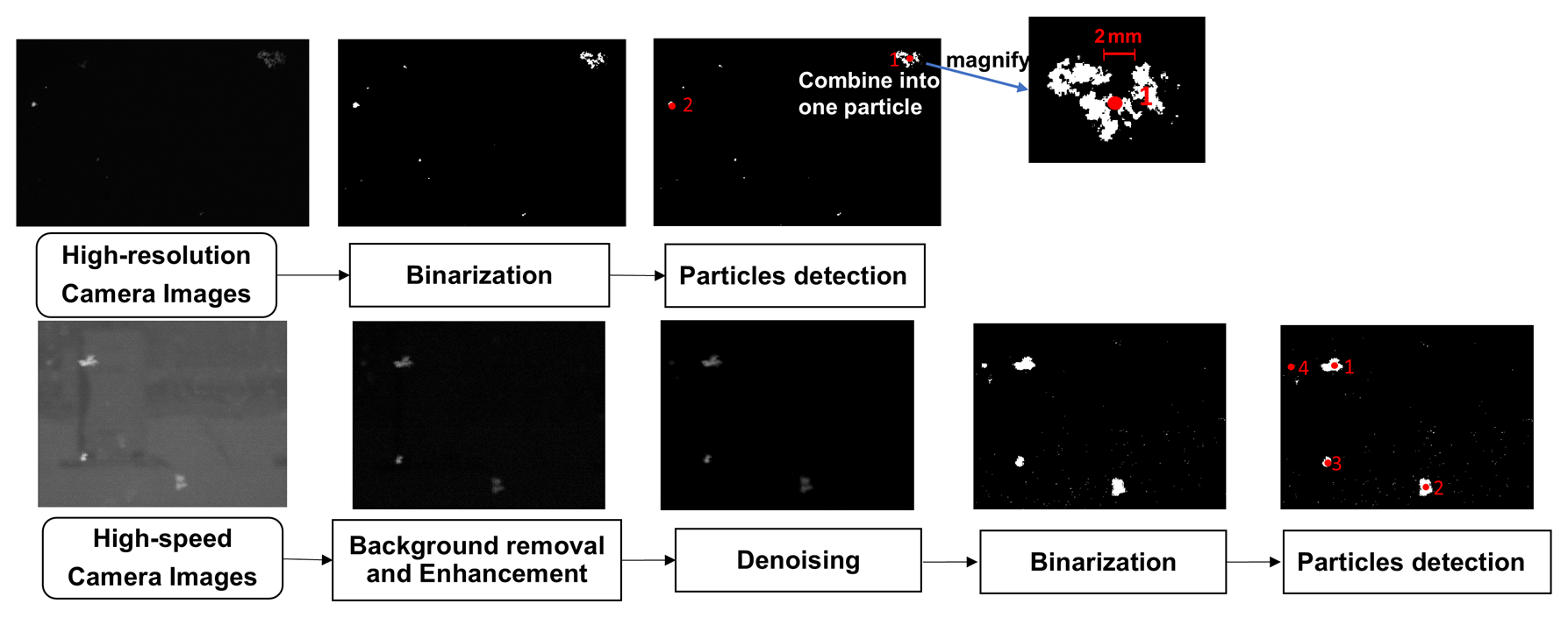
For high-resolution camera images with a resolution of 4096 × 3000, no background removal and denoising are required due to low image noise and little background interference. The processing steps are as follows:

• i.

  Image binarization. The image is binarized through adaptive thresholding, which is a method used to binarize images by determining thresholds locally rather than using a global threshold. This approach is particularly useful for images with varying illumination and complex backgrounds (Bataineh et al., 2011). The threshold at each pixel (u, v), denoted as T(u, v), is calculated based on the local mean intensity μ(u, v) of the pixels in a defined neighborhood around (u, v). This local mean is adjusted by a sensitivity coefficient C to balance the classification of pixels into foreground or background.

  $$\begin{array}{}\text{(3)}& T(u,v)=\mathit{\mu }(u,v)-C\end{array}$$

  The sensitivity coefficient C is crucial; it adjusts how the local mean is used to set the threshold. A smaller C favors classifying pixels as foreground, while a larger C favors background classification. We manually adjusted the sensitivity coefficient C to determine the optimal value of 0.4. This process involved visually assessing the binarization outcomes for various C values to identify which value best distinguishes between foreground objects and background objects.

• ii.

  Particle detection. Firstly, in binarized images, detect the connected regions with an area larger than 20 px (equivalent to 0.035 mm², where diameter is about 0.2 mm), which enables the removal of pixel noise or small snowflakes (no larger than 20 px) from the image, to exclude features of small snowflakes that cannot be detected from the analysis. Secondly, combine regions into a single region of interest (ROI) when the distance between the closest points of connected regions in a single image is detected to be less than 0.5 mm apart. This step is necessary because a single particle may sometimes be perceived as two separate particles due to its position near the edge of the image processing threshold. This method enhances the accuracy of foreground particle detection, particularly in images with complex backgrounds and uneven illumination. Thirdly, discard the blurred particles outside the depth of field. To avoid detecting the particles completely out of focus, in the greyscale image before binarization, the mean gray value of the ROI must be at least 20 times greater than the mean gray value of the image, and the variance of the Laplacian of the ROI gray value must be at least 10 times greater. Fourthly, discard the particles at the edge of the image. If the connected region of a particle contains points located at the edges of the image, the particle is considered not to be fully captured, and it should be discarded.

For the high-speed camera images with a resolution of 720 × 540, there is non-negligible noise and background interference; therefore, two more steps are required before image binarization and particle detection:

• i.

  Background removal and enhancement. Background artifacts captured by high-speed cameras in natural settings can be influenced by varying lighting conditions, lens surface contamination, or other factors that change over time. To address this issue, a real-time background detection method is employed. Specifically, 1024 images are randomly selected every minute to calculate the average grayscale value, representing the minute-by-minute background changes. These background variations are then subtracted from all images taken within that minute to effectively remove the background interference. It is further necessary to enhance the contrast of the image by stretching the grayscale histogram to better distinguish between background and foreground particles.

• ii.

  Image denoising. Median filtering is used to remove the remaining noise. Further, the image binarization and particle detection methods are the same as the previous high-resolution camera image processing methods.

The two types of image processing processes and the results of each step are shown in Fig. 6.

Figure 6 Flowchart of two types of image processing.

The next step is to evaluate the effectiveness of the image processing algorithm. Firstly, drop the 15 spheres with absolute sphericity ranging from 1 to 25 mm in diameter into the OV of the 3D-PPI, and acquire 20 clear images for each diameter (Fig. 7a). The materials of the spheres have a similar refractive index to the snowflakes. Next, use the image processing algorithm to convert the sphere image into the binarized image (Fig. b), and then calculate D_max and D_eq. (In the image, D_max is the diameter of the smallest enclosing circle, and D_eq is the diameter of the circle equal to the area of the particle profile. D_max and D_eq are equal only when the image of the sphere is perfectly circular.) Finally, convert D_max and D_eq from pixels to millimeters through pixel resolution (41.6 µm px⁻¹), and calculate the average value of D_max and D_eq 20 times for each diameter.

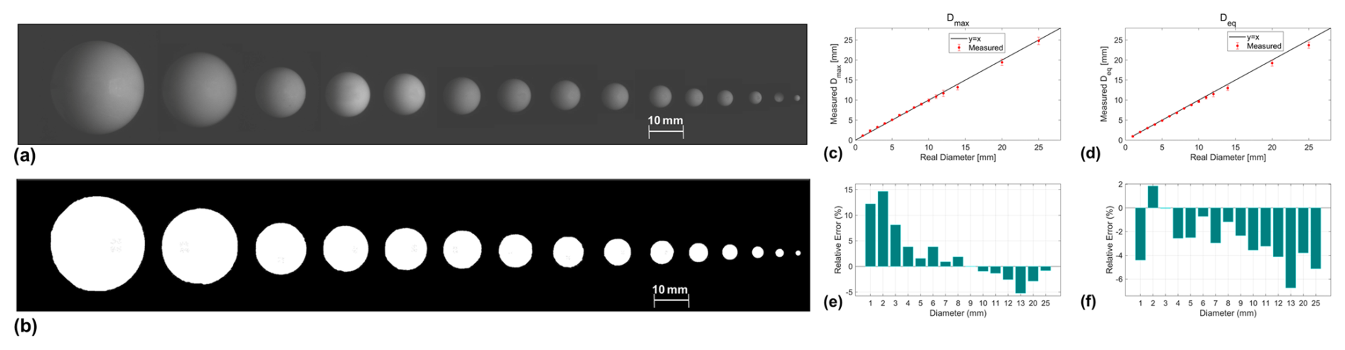
Figure 7 (a) The 15 reference spheres ranging from 1 to 25 mm in diameter captured by the high-resolution camera. (b) The binarized images of 15 spheres after image processing; the average values of measurements of D_max. (c–f) The average values and relative errors of 20 D_max and D_eq measurements per diameter sphere.

Regarding the D_max measurement results (Fig. 7c, e), smaller spheres (≤ 9 mm) exhibit slight overestimations of the true values, while larger particles show underestimations. The maximum relative error is approximately 14 %. The arithmetic mean of relative errors across all diameters is +2.2 %, though the average absolute relative error (i.e., magnitude regardless of sign) is 5.0 %, reflecting a systematic overestimation tendency. For D_eq measurements (Fig. 7d, f), nearly all estimates are below the true values, with a single exception at 10 mm (+0.8 %). The worst relative error is −7 %, and the arithmetic mean of relative errors is −2.7 %. The consistent underestimation of D_eq (except for the 10 mm case) suggests its utility for systematic error correction. Overall, the image processing methods demonstrate effectiveness, with errors remaining minimal in practical terms.

4.2 Particle matching and localization

4.2.1 Particle matching

In the observation volume of the 3D-PPI, there might be numbers of particles with similar sizes, colors, shapes, and textures, which poses a challenge for particle matching from the images captured by the three cameras. In this work, we propose a particle matching algorithm that addresses this issue by focusing on the spatial positions of particles in three images, as derived from the projection matrices obtained through precise calibration of the trinocular telecentric camera system. For one particle, the matching algorithm is implemented in detail as follows (Fig. 8):

• i.

  Detect the centroid coordinates of the particle P (u, v) in the PCS from Cam0 (Fig. 9a).

• ii.

  Using the projection matrix KM₀ of Cam0, the underdetermined linear equations corresponding to P are solved to obtain a straight line L in the WCS. Specifically, it is equivalent to solving W₁ in Eq. (2) with KM and C₁ known, where the solution to W₁ is not unique and all solutions are L in the WCS. L represents all points in 3D space that can be projected onto P by KM₀; in other words, the line L is the back projection of the point P in the WCS.

• iii.

  Project L onto the planes of Cam1 and Cam2 by multiplying the projection matrices KM₁ and KM₂, respectively, with L, resulting in the line segments on each of the image planes of Cam1 and Cam2 (Fig. 9b, c). The exact derivations of the formulae in (i) and (ii) are described in detail in Appendix B.

• iv.

  Detect the particles that the line segments pass through on Cam1 and Cam2. If the line segments do not pass through any particles in Cam1 or Cam2, it is a failed matching, meaning that the particle does not appear in the effective OV.

Figure 8 Flowchart of a particle matching.

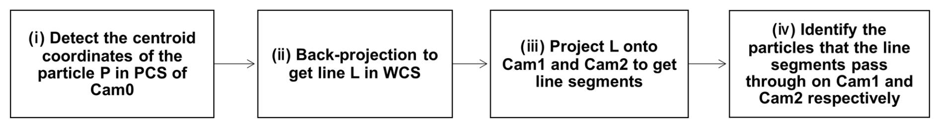
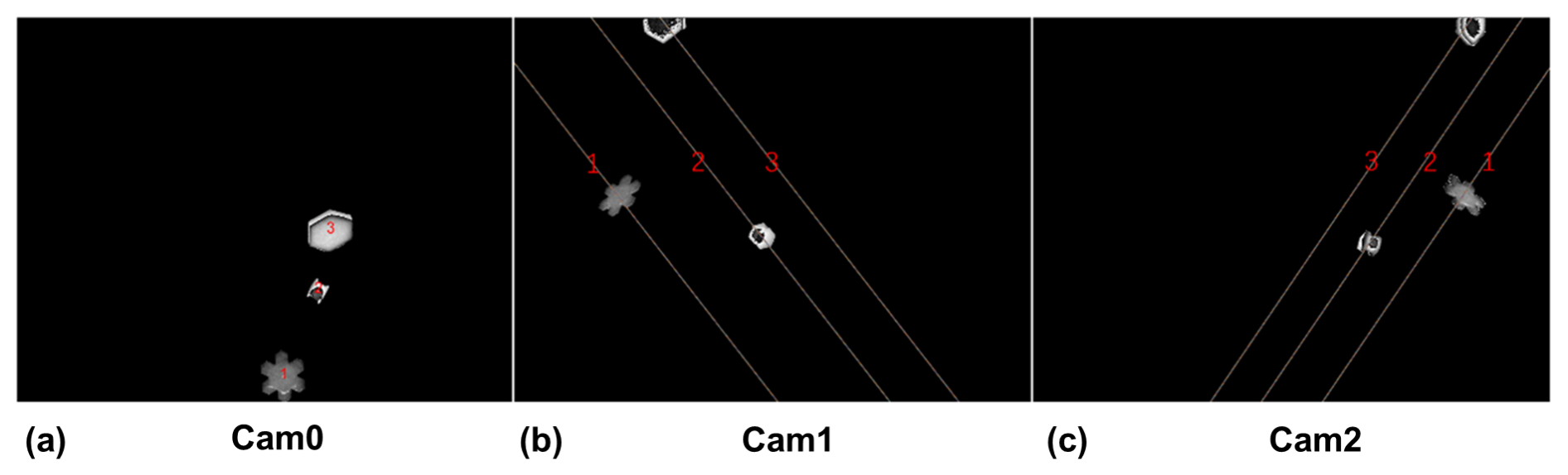
Figure 9 The three particles detected in Cam0 can only appear on the corresponding three line segments in Cam1 and Cam2.

By performing the above matching for each particle detected by Cam0, the location of this particle in Cam1 and Cam2 can be found. Figure 10 shows the three particles detected in Cam0 and the matching of each particle in Cam1 and Cam2.

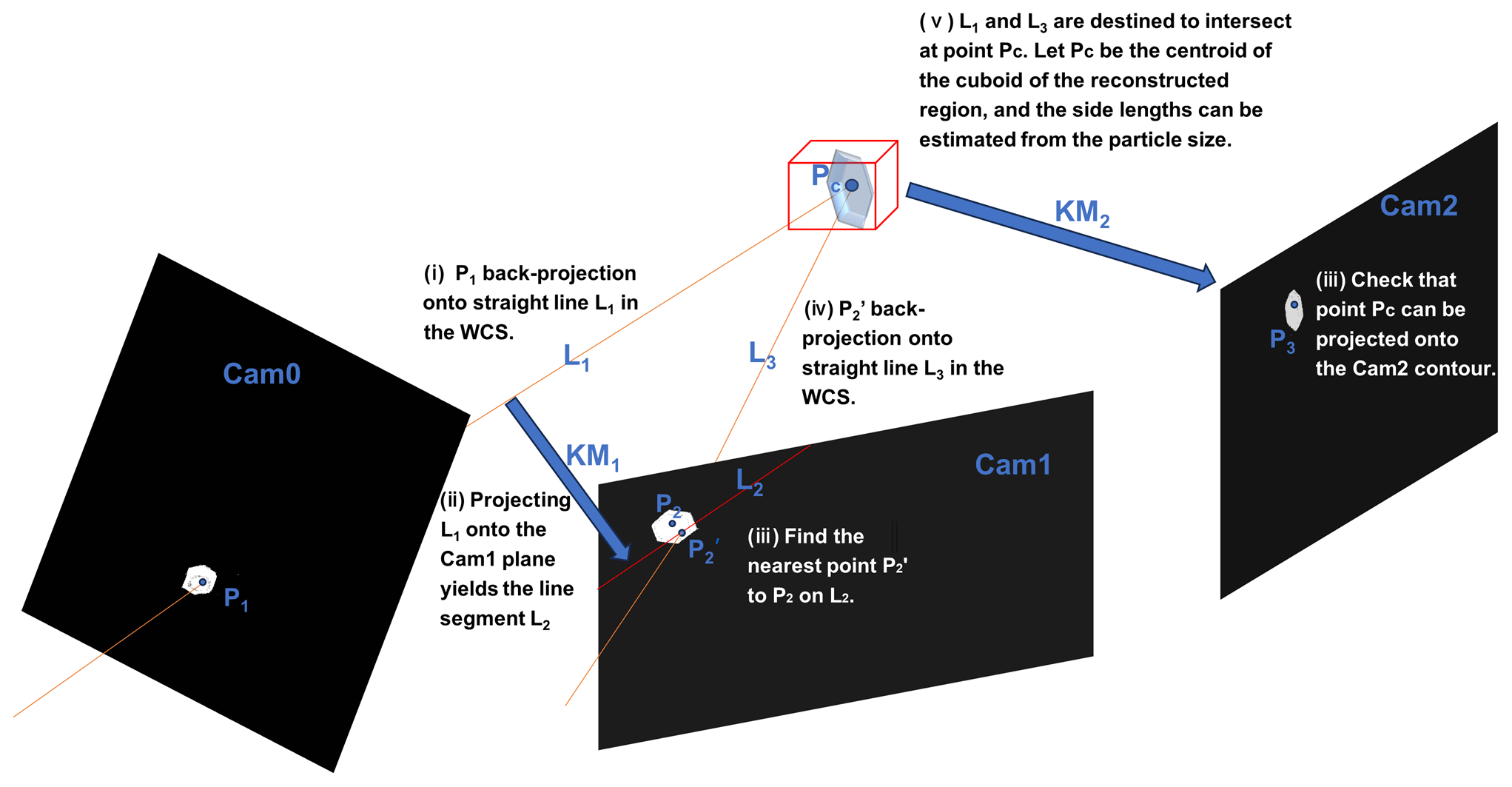
Figure 10 Steps to localize the particle position in the WCS according to the image particle contours.

4.2.2 Particle localization

After completing camera calibration and particle matching, 3D reconstruction for each particle needs to be performed. However, since each particle only occupies a small space in the effective OV, we propose a method that involves preliminarily locating particles in the WCS before proceeding with subsequent 3D reconstruction. This method leverages the positions of single particles in three images to identify the minimal cuboid capable of containing the particles, thereby accurately pinpointing the particles' localizations.

For a single particle, the pixel coordinates of the centroid point of the particle in Cam0, Cam1, and Cam2 have been detected, and the subsequent 3D spatial localization steps in the WCS are as follows (Fig. 10):

• i.

  Find the back-projection line L₁ of point P₁ by KM₀. The underdetermined linear equation corresponding to P₁ is solved to obtain a straight line L₁ in the WCS. This implementation principle is similar to the second step of particle matching mentioned above. Equations (B1) and (B2) in Appendix B explain this process.

• ii.

  The lines L₁ are projected onto the planes of Cam1 by multiplying the projection matrices KM₁, resulting in line segment L₂, which is represented as a two-row by one-column matrix. This corresponds to the segment of L_p1 within the image boundaries, as described in Eq. (B3).

• iii.

  Find the point $P_{\mathrm{2}}^{\prime }$ on L₂ that is closest to P₂. Due to the irregular shape of the particle, $P_{\mathrm{2}}^{\prime }$ does not necessarily coincide with P₂.

• iv.

  Follow the same approach as in step 1 – determine the back-projection line L₃ of point $P_{\mathrm{2}}^{\prime }$ by KM₁.

• v.

  Localize the 3D coordinates of the intersection of L₁ and L₃ in the WCS, that is P_c, which is the centroid of the target cuboid, and further determine the side lengths of the cuboid. From the previous steps, L₁ and L₃ are destined to intersect in the WCS, and the intersection point is regarded as the centroid of the rectangle, whose side lengths can be determined by converting from the pixel dimensions in the particle image to the actual physical dimensions in the WCS.

• vi.

  Finally, verify that the projection of point P_c through KM₂ in Cam2 is near point P₃ and within the particle contour; otherwise, it is a failed localization.

The particle's position in the WCS should be inside the region of the cuboid determined by localization, which is next discretized into numerous smaller voxel grids to finely perform the 3D reconstruction.

4.3 Three-dimensional (3D) reconstruction

The visual hull (VH) method is a technique used to reconstruct the 3D shape of snowflakes by utilizing silhouettes, which are the outlines of the snowflakes as seen from different camera angles. In this process, multiple cameras are positioned around the snowflake at various viewpoints (Cam0, Cam1, and Cam2 in 3D-PPI). Each camera captures the silhouette of the snowflake, and these silhouettes are carefully calibrated to ensure that they accurately represent the snowflake's geometry. A cone of the silhouette is created by back projecting the set of points of view of the previously detected silhouettes into the corresponding image planes in front of the cameras (Fig. 3b), and the intersection of these cones gives the visual hull (Hauswiesner et al., 2013). Since concave features do not affect the silhouette obtained from each image, a limitation of the visual hull method is its inability to capture concave features. Based on high-resolution contour images captured by the three high-resolution cameras of the 3D-PPI and the projection matrix for each camera, we propose applying the visual hull method to reconstruct the 3D shapes of snowflakes. The use of telecentric cameras allows the visual solid cones formed by back projection to become visual solid columns (Fig. 3b, d).

The algorithm operates as follows: given a multi-viewpoint contour image and projection matrices, it ascertains whether the pixel or voxel corresponding to a spatial point on each contour map is part of the object's contour. The resulting model represents a sample of the smallest convex set that encloses the object's true shape, precluding the depiction of indentations.

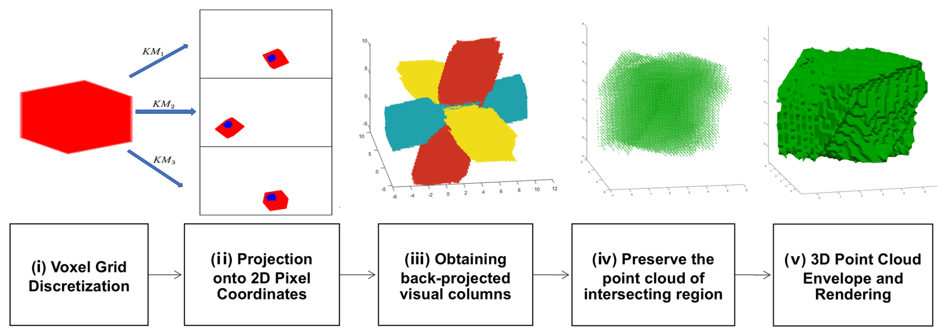
Initially, we employ the preliminary particle localization method described in Sect. 4 to estimate the particle's approximate spatial position. The further procedure for obtaining a 3D point cloud and reconstructing the 3D model of precipitation particles is outlined through the following refined steps (Fig. 11):

• i.

  Voxel grid discretization. Subdivide the space into a voxel grid with a predefined resolution. For each voxel, extract the 3D coordinates of the upper-left corner point. This grid will serve as a framework for subsequent steps.

• ii.

  Projection onto 2D pixel coordinates. Utilize the projection matrix to project the 3D voxel coordinates of each voxel onto the three-angle contour, transforming them into 2D pixel point coordinates.

• iii.

  Obtaining back-projected visual columns (by three sets of point clouds). Mark the 3D voxel coordinates of points that can be projected onto the contours of each of the three images; that is, obtain three contours of back-projected visual columns.

• iv.

  Preserve the point cloud of the intersecting region. Retain a point cloud within the convergence region of the three optical axes, identifying the spatial locus where the 3D reconstructed object is situated.

• v.

  3D point cloud envelope and rendering. Apply the triangular sectioning algorithm to extract the visual envelope of the 3D point cloud. Subsequent rendering steps will then be used to construct the 3D reconstruction model of the precipitation particle.

Figure 11 Flowchart of 3D construction algorithm.

5 Preliminary results of field experiment

5.1 Case studies of snowfall case

To evaluate the performance of the 3D-PPI, the prototype of the 3D-PPI was deployed at Tulihe, China (50.692° N, 121.652° E; 733 m a.m.s.l.), from 1 January 2024, and an OTT Parsivel laser disdrometer (OTT for short) was installed 10 m apart for comparison. According to the conclusion of the wind field simulation in Appendix C, the 3D-PPI is installed facing towards the south. A typical snowfall case lasting 13 h, from 19:00 UTC on 28 March 2024 to 07:59 UTC on 29 March 2024, was observed and analyzed.

The PSD calculated from OTT counting is as follows (Zhang et al., 2019):

$$\begin{array}{}\text{(4)}& \text{PSD}\left(D_i\right)={\displaystyle \frac{\mathrm{1}}{S\cdot T\cdot \mathrm{\Delta }{D}_i}}\sum _{j=\mathrm{1}}^{\mathrm{32}}{\displaystyle \frac{n_{ij}}{V_j}},\end{array}$$

where PSD (D_i) (mm⁻¹ m⁻³) is the number concentration of particles per unit volume per unit size interval ΔD_i for snowflake size D_i (mm), n_ij is the number of snowflakes within size bin i and velocity bin j, T (s) is the sampling time (60 s in this study), V_j (m s⁻¹) is the falling speed for velocity bin j, and S (m²) is the effective sampling area (0.18 m × 0.03 m).

The time-averaged PSD calculated from the 3D-PPI counting over a specified period is as follows:

$$\begin{array}{}\text{(5)}& \text{PSD}\left(D_i\right)={\displaystyle \frac{N_i}{\mathrm{\Delta }{D}_i\cdot N_{\mathrm{ima}}\cdot V_i}},\end{array}$$

where N_i is the number of particles in the ith size bin, and N_ima is the number of acquired images over a period of time. The size descriptor D for the 3D-PPI is D_max or D_eq in this paper, and V_i (m³) is the valid OV of Cam0 after edge correction. Since we discard particles at the edges of the image in Sect. 4.1, V_i is a function of D_i, shown in Eq. (6). Here, a, b, and d represent the length (0.17 m), width (0.125 m), and depth (0.088 m) of the field of view, respectively.

$$\begin{array}{}\text{(6)}& V_i=\left(a-D_i\right)\cdot \left(b-D_i\right)\cdot d\end{array}$$

Considering that the sampling rate of a high-resolution camera is 5 fps and the time for a snowflake to pass through the field of view is less than 0.2 s, the probability of capturing the same snowflake in two consecutive frames is low.

During the snowfall case, three high-resolution cameras of the 3D-PPI recorded 552 383 and 328 792 snowflakes over 2 d. The time-averaged PSD in the same period obtained by the 3D-PPI (using two types of size descriptors) and OTT are compared (Fig. 12a, b). The PSDs measured by OTT and the 3D-PPI using D_eq as a size descriptor are highly consistent; however, they deviate significantly from those using D_max as a size descriptor. The PSDs of particles with a D_eq of about 0.4 mm were the highest for both chosen days.

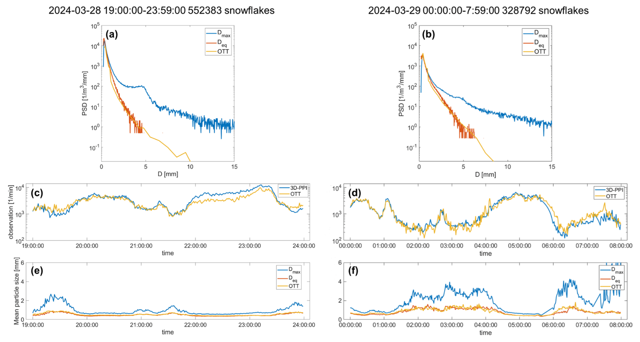
Figure 12 This typical continuous snowfall was split into 2 d and plotted separately (left and right). The 1 min particle size distribution (PSD) of D_max (blue) and D_eq (orange) for the 3D-PPI and OTT (yellow) for the snowfall case (a, b). Temporal plot of average particle counts per unit volume per minute over 2 d (c, d). Temporal plot of average particle size per minute over time (e, f).

The trends in the number density of particles observed by the two instruments were similar; the correlation coefficients are 0.94 and 0.96 for the 2 d. In comparing the temporal plots (Fig. 12c, d, e, f), certain periods (19:00 to 19:50, 20:50 to 22:00, and after 23:30 UTC on 28 March; 01:30 to 04:30 and 06:00 to 07:59 UTC on 29 March) exhibited a smaller number of particles per unit volume, with larger average sizes and greater difference between D_eq and D_max. This indicates a higher degree of aggregation and potentially more complex shapes of individual snowflakes during these times. Conversely, other periods (19:50 to 20:50 and 22:00 to 23:30 UTC on 28 March; 00:00 to 01:30 and 04:30 to 06:00 UTC on 29 March) showed a larger number of particles per unit volume, smaller average sizes, and reduced difference between D_eq and D_max.

5.2 Three-dimensional shape of snowflakes

Figure 14 shows the reconstructed 3D shapes of six snowflakes collected on 6 April 2024. For each snowflake, three images were obtained from three high-resolution cameras (Cam0, Cam1, and Cam2), and the results of the 3D shape were reconstructed by utilizing the visual hull method (Fig. 13). To characterize the 3D shape of each snowflake, four parameters are calculated: volume (V), dimensional maximum in volume (DV_max; distance between the two farthest points on the surface of the 3D reconstructed particle), aspect ratio (AR; ratio of the longest and shortest axes of the smallest outer ellipsoid), and sphericity (Sp). Sp is derived from V and S (surface area of 3D reconstructed hull) and characterizes the degree to which 3D particles approach the sphere:

$$\begin{array}{}\text{(7)}& \text{Sp}={\displaystyle \frac{\mathrm{4}\mathit{\pi }{\left(\frac{\mathrm{3}V}{\mathrm{4}\mathit{\pi }}\right)}^{\frac{\mathrm{2}}{\mathrm{3}}}}{S}}.\end{array}$$

The 3D shapes of snowflakes ranging in volume from over 400 mm³ (Fig. 14b) to as small as less than 20 mm³ (Fig. 13f) can all be reconstructed. In the algorithm when two connected regions are close together, they are considered to be the same snowflake, so the reconstructed snowflake will appear as a separated small part that is not connected to the main body, in which case DV_max is meaningless (Fig. 13e, f). From the results, it can be found that the visual hull approach can effectively and precisely execute the 3D reconstruction for snowflakes with highly realistic, intricate, and varied shapes and compositions, as well as diverse sizes and sphericity. While individual snowflake analysis is beyond the scope of this study, the reconstructed 3D shapes (Fig. 13) demonstrate the instrument's capability to resolve diverse morphologies. Therefore, the next step is to embed the 3D reconstruction and pre-algorithms into the instrument to realize real-time, automated, and batch 3D reconstruction of snowflakes to statistically characterize the distribution of the 3D shape of a large number of snowflakes.

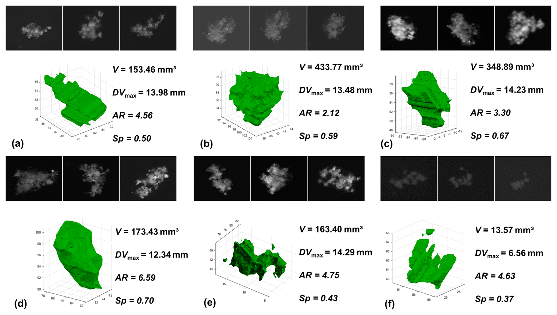
Figure 13 Several typical snowflakes captured by the 3D-PPI in the field and the corresponding 3D reconstruction results. For each reconstruction, the computed V, DV_max, AR, and Sp are shown.

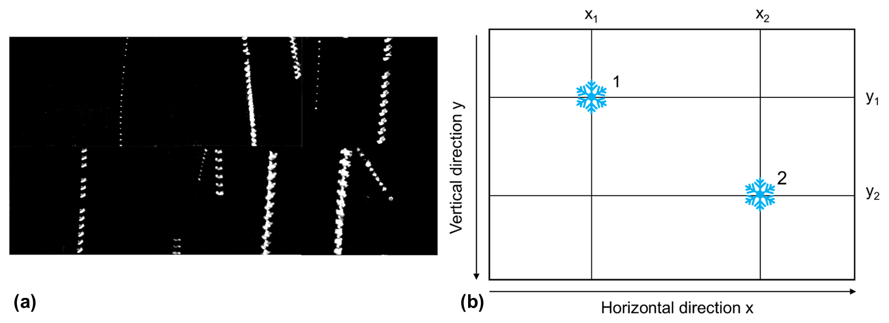
Figure 14 (a) Processed high-speed camera images, with the same particles from consecutive frames merged into a single image. (b) Speed measurement schematic.

5.3 Fall velocity of snowflakes

The exposure time for a single frame is 20 µs, which renders the motion blur of the particles negligible. Additionally, the time interval between two consecutive frames is 5 ms, allowing the same particle to be captured multiple times, thus enabling accurate velocity calculations. The same particle from consecutive frames is merged into a single image in Fig. 14a to enhance the visualization of its movement. The speed calculation schematic is shown in Fig. 14b.

When there are multiple particles in a high-speed camera image, particle matching is required. The particle is regarded as the same particle when the following two principles are satisfied: (i) the pixel coordinates of the centroid of the contours in the particle images in consecutive frames are similar (the falling velocity of the snowflake is generally not more than 4 m s⁻¹, so the distance between the vertical pixel coordinates of the same particle centroid in two adjacent image frames is not more than 100 px), and (ii) given that the size of the particles captured in two consecutive frames does not change significantly, D_max and D_eq of the particles are similar, generally not more than 20 % (the D_max or D_eq value of the particle in the next frame deviates within ±20 % of the previous particle). Each particle may have recorded anywhere from 2 to 20 D_max, D_eq, pixel horizontal coordinates, and pixel vertical coordinates. The standard deviation of D_max and D_eq and the difference between the horizontal and vertical coordinates of each particle are calculated, and if the standard deviation of any of the particle's quantities is too large, the particle is treated as an invalid particle, and it will be discarded. D_max and D_eq of each particle are taken to be the maximum of these values, which excludes cases where the particle is not captured because it is at the edge of the image. The horizontal velocity (V_h) component and vertical velocity component (V_v) are calculated as follows:

$$\begin{array}{}\text{(8)}& {\displaystyle }{V}_{\mathrm{h}}={\displaystyle \frac{x_{\mathrm{2}}-x_{\mathrm{1}}}{\mathrm{\Delta }t}}\cdot \mathit{\alpha },\text{(9)}& {\displaystyle }{V}_{\mathrm{v}}={\displaystyle \frac{y_{\mathrm{2}}-y_{\mathrm{1}}}{\mathrm{\Delta }t}}\cdot \mathit{\alpha },\end{array}$$

where x₂, x₁ and y₂, y₁ denote the horizontal and vertical coordinates of the same particle in two consecutive frames; Δt denotes the time interval, which is generally 5 ms; and α denotes the pixel resolution of the high-speed camera at the working distance, which is 265 µm px⁻¹.

From 08:00 to 08:30 UTC on 6 April 2024, Cam3 of the 3D-PPI recorded 77 042 valid snowflakes, and for each snowflake, horizontal and vertical velocities were calculated. The distributions of horizontal and vertical velocity components as a function of D_eq are further plotted as a scatter density plot and compared to the results measured by OTT at the same period, which is shown in Fig. 15. The color scale denotes the number of snowflakes measured in the corresponding bins. OTT's D and V binning is uneven, whereas here the 3D-PPI is set to even binning, with D and V intervals of 0.1 mm and 0.1 m s⁻¹, respectively. The solid red and black lines in Fig. 15b, d represent the empirical curves of the falling velocity and diameter of unrimed aggregates and densely rimed dendrites, respectively (Locatelli and Hobbs, 1974).

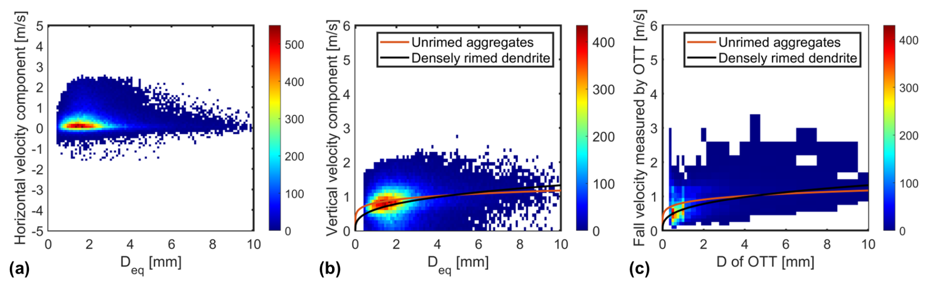
Figure 15 Distribution of (a) horizontal and (b) vertical snowflake velocities with D_eq measured by the 3D-PPI. Distribution of falling velocity with diameter measured by (c) OTT. The color scale denotes the number of snowflakes measured.

The empirical velocity of unrimed aggregates is

$$\begin{array}{}\text{(10)}& V_{\mathrm{1}}=\mathrm{0.81}{D}^{\mathrm{0.16}}.\end{array}$$

The empirical velocity of densely rimed dendrites is

$$\begin{array}{}\text{(11)}& V_{\mathrm{2}}=\mathrm{0.62}{D}^{\mathrm{0.33}}.\end{array}$$

Installing the instrument facing south means that the horizontal velocity seen by the high-speed camera Cam3 corresponds to east–west. The average value of the horizontal velocity measured by the 3D-PPI is +0.41 m s⁻¹, and the standard deviation is 0.73 m s⁻¹ (Fig. 15a). The overall distribution of particle horizontal velocities ranges between ±3 m s⁻¹, and more than 70 % of the snowflakes have a horizontal velocity distribution between ±1 m s⁻¹. Positive velocities predominate over negative ones, largely influenced by the prevailing westward winds. The average value of the vertical velocity component measured by the 3D-PPI is 0.74 m s⁻¹, and the standard deviation is 0.62 m s⁻¹, while the average value and standard deviation of the velocities measured by OTT are 0.69 and 0.31 m s⁻¹. The diameters of snowflakes measured by the 3D-PPI (OTT) were concentrated in the range of 0.5 to 2.2 mm (0.4 to 1 mm). The vertical velocities were concentrated in the range of 0.6 to 1.1 m s⁻¹ (0.3 to 0.7 m s⁻¹). The diameter and velocity values measured by the 3D-PPI are larger and more dispersed than those measured by OTT. Overall, the vertical velocity of snowflakes increases with increasing diameter, and the observed data are in good agreement with the two empirical velocity relationships (Locatelli and Hobbs, 1974). It should be noted that small numbers (7 % of the total sample) of small snowflakes have an almost zero vertical velocity or are negative (not shown due to the positive vertical-axis range of Fig. 15b). This phenomenon may be attributed to localized updrafts caused by thermal convection or wind shear. Additionally, lighter or smaller snowflakes may be temporarily suspended in the air due to turbulence, resulting in a recorded velocity of almost zero or upwards.

6 Conclusion

The design of the Three-Dimensional Precipitation Particle Imager (3D-PPI) was introduced in this paper. The 3D-PPI consists of three high-resolution cameras (4096 × 3000, 5 fps) with telecentric lenses and one high-speed camera (720 × 540, 200 fps) with a non-telecentric lens. The three high-resolution cameras are oriented at a 45° angle relative to the optical axis of the high-speed camera, forming an intersecting observation volume of 775 cm³. The high-resolution cameras feature a pixel resolution of 41.6 µm px⁻¹ and are precisely synchronized by clock control, which is sufficient to obtain fine shapes of snowflakes larger than 0.2 mm, and the large field of view of 170 mm × 125 mm enables the cameras to capture enough snowflakes to estimate PSD accurately. The high-speed camera allows for the calculation of velocity accurately. Moreover, the utilization of telecentric lenses eliminates the sizing error caused by the uncertain distance between the snowflakes and the cameras.

For the three high-resolution cameras, a calibration method using a 3D checkerboard was proposed. By shooting the 3D checkerboard grid from three angles simultaneously, we found the correspondence between the world coordinate points and the image coordinate points and then solved the system of equations to estimate the projection matrix of the three high-resolution cameras. A reprojection averaging error of 0.32 px can indicate the accuracy of the calibration. However, even minor displacements of the cameras can alter the projection matrix, which may adversely affect the subsequent reconstruction results. Therefore, it is essential to perform periodic calibration to ensure the accuracy and reliability of the projection matrix. Both types of image processing require binarization and particle detection, and high-speed cameras require background removal, enhancement, and denoising before these two steps. The image processing algorithm needs to be evaluated by batch processing of ceramic sphere images, and the average values of the relative errors of D_max and D_eq are +2.2 % and −2.7 %, respectively. The issue of matching the same particle by its position in the image can be addressed by using the projection matrix obtained from the calibration of cameras in Sect. 3.1. The preliminary determination of the 3D spatial localization of particles after particle matching can effectively improve the computational efficiency of the 3D reconstruction algorithm, so particle localization is an indispensable step before 3D reconstruction. The snowflake 3D shape is further reconstructed using a visual hull algorithm based on binarized contour images from different angles and projection matrixes (Kleinkort et al., 2017).

The 3D-PPI was installed at Tulihe, China, on 1 January 2024, and the OTT was installed 10 m apart for comparison. The PSDs, 3D shapes, and fall velocity of snowflakes were preliminarily analyzed. The PSD measured solely by Cam1 and that obtained by OTT exhibit excellent agreement during the typical snowfall case. Several snowflakes with different morphologies were selected and reconstructed in three dimensions, indicating that the 3D-PPI is initially capable of reconstructing snowflakes. The horizontal and vertical velocities of snowflakes were calculated to obtain the velocity distribution. Further comparisons were made with the OTT, and overall, the two distributions for fall velocity were similar. However, the diameter and velocity values measured by the 3D-PPI are larger and more dispersed than those measured by OTT. This difference may be attributed to the potential magnification differences in the high-speed camera in the 3D-PPI due to particles being at varying distances from the cameras.

In this paper, the PSD statistics use only one image from a high-resolution camera, and the 3D reconstruction is limited to just one case study. Future work will focus on algorithm optimization for real-time 3D reconstruction and statistical characterization of snowflake shape distributions. Moreover, the accuracy of velocity measurement still needs to be verified and improved. In the future, the 3D-PPI will facilitate more precise and realistic estimations of snowflake parameters, including the size, volume, mass, and density. Based on these parameters, the 3D-PPI has the potential to improve radar-based estimation of solid precipitation in winter.

Appendix A: Coordinate system transformation

Camera calibration encompasses four key coordinate systems:

• 1.

  World coordinate system (WCS). This system, denoted as (X_w, Y_w, Z_w), is a user-defined 3D spatial coordinate system that is utilized to describe the location of the target object within the tangible world, with units typically expressed in millimeters.

• 2.

  Camera coordinate system (CCS). This coordinate system, denoted as (X_c, Y_c, Z_c), is intrinsic to the camera and is utilized to describe the object's position relative to the camera's perspective. It acts as an intermediary between the WCS and the image (pixel) coordinate system.

• 3.

  Image coordinate system (ICS). This system, denoted as (x, y), is employed to articulate the projection and translation of the object from the CCS to the ICS during the imaging process. It facilitates the subsequent extraction of coordinates under the pixel coordinate system, with the unit being millimeters.

• 4.

  Pixel coordinate system (PCS). This system, denoted as (u, v), describes the coordinates of the object's image point post-imaging on the digital image sensor. It is the actual coordinate system from which image information is read from the camera, measured in units of pixels.

The camera imaging process involves the transformation from the WCS to the PCS. Camera calibration, in essence, is the procedure of determining the transformation relationships between these four coordinate systems.

A1 WCS to CCS

Firstly, the transformation of a camera shot from the WCS to the CCS is a rigid-body transformation, where the object does not deform but only rotates and translates. Only the rotation matrix R and translation matrix T need to be obtained. The camera coordinate system is obtained by rotating θ, α, and β angles around the z, y, and x axes in turn and translating to obtain the rotation matrix in the three dimensions:

$$\begin{array}{}\text{(A1)}& \begin{array}{rl}& R_z\left(\mathit{\theta }\right)=\left[\begin{array}{ccc}\cos \left(\mathit{\theta }\right)& \sin \left(\mathit{\theta }\right)& \mathrm{0}\\ -\sin \left(\mathit{\theta }\right)& \cos \left(\mathit{\theta }\right)& \mathrm{0}\\ \mathrm{0}& \mathrm{0}& \mathrm{1}\end{array}\right]\\ & R_y\left(\mathit{\beta }\right)=\left[\begin{array}{ccc}\cos \left(\mathit{\beta }\right)& \mathrm{0}& -\sin \left(\mathit{\beta }\right)\\ \mathrm{0}& \mathrm{1}& \mathrm{0}\\ \sin \left(\mathit{\beta }\right)& \mathrm{0}& \cos \left(\mathit{\beta }\right)\end{array}\right]\\ & R_x\left(\mathit{\alpha }\right)=\left[\begin{array}{ccc}\mathrm{1}& \mathrm{0}& \mathrm{0}\\ \mathrm{0}& \cos \left(\mathit{\alpha }\right)& \sin \left(\mathit{\alpha }\right)\\ \mathrm{0}& -\sin \left(\mathit{\alpha }\right)& \cos \left(\mathit{\alpha }\right)\end{array}\right].\end{array}\end{array}$$

The three matrices are multiplied together to obtain a 3D rotation matrix:

$$\begin{array}{}\text{(A2)}& \begin{array}{rl}& \mathbf{R}=R_x\left(\mathit{\alpha }\right)R_y\left(\mathit{\beta }\right)R_z\left(\mathit{\theta }\right)=\\ & \left[\begin{array}{ccc}\cos \left(\mathit{\beta }\right)\cos \left(\mathit{\theta }\right)& \cos \left(\mathit{\beta }\right)\sin \left(\mathit{\theta }\right)& -\sin \left(\mathit{\beta }\right)\\ -\cos \left(\mathit{\alpha }\right)\sin \left(\mathit{\theta }\right)+\sin \left(\mathit{\alpha }\right)\sin \left(\mathit{\beta }\right)\cos \left(\mathit{\theta }\right)& \cos \left(\mathit{\alpha }\right)\cos \left(\mathit{\theta }\right)+\sin \left(\mathit{\alpha }\right)\sin \left(\mathit{\beta }\right)\sin \left(\mathit{\theta }\right)& \sin \left(\mathit{\alpha }\right)\cos \left(\mathit{\beta }\right)\\ \sin \left(\mathit{\alpha }\right)\sin \left(\mathit{\theta }\right)+\cos \left(\mathit{\alpha }\right)\sin \left(\mathit{\beta }\right)\cos \left(\mathit{\theta }\right)& -\sin \left(\mathit{\alpha }\right)\cos \left(\mathit{\theta }\right)+\cos \left(\mathit{\alpha }\right)\sin \left(\mathit{\beta }\right)\sin \left(\mathit{\theta }\right)& \cos \left(\mathit{\alpha }\right)\cos \left(\mathit{\beta }\right)\end{array}\right],\end{array}\end{array}$$

where, for z, y, and x, the direction of rotation is followed by the right-hand spiral rule; the thumb points to the direction of the axis; and the four-finger direction is the positive direction of rotation.

Following the application of the rotation matrix R, the WCS and CCS share identical orientations. To achieve full alignment between the two systems, an additional translation via T is required to reconcile their origins.

The rotation and translation process can be expressed by the following formula:

$$\begin{array}{}\text{(A3)}& \left[\begin{array}{c}{X}_c\\ Y_c\\ Z_c\\ \mathrm{1}\end{array}\right]=\left[\begin{array}{cc}{R}_{\mathrm{3}\times \mathrm{3}}& T_{\mathrm{3}\times \mathrm{1}}\\ O& \mathrm{1}\end{array}\right]\left[\begin{array}{c}{X}_w\\ Y_w\\ Z_w\\ \mathrm{1}\end{array}\right].\end{array}$$

A2 CCS to ICS

The difference between telecentric cameras and traditional pinhole cameras is the difference in projection. A pinhole camera uses a perspective projection to transform from the CCS to the ICS; a telecentric camera uses an orthogonal projection. The relationship between the CCS and ICS is as follows:

$$\begin{array}{}\text{(A4)}& \left[\begin{array}{c}x\\ y\\ \mathrm{1}\end{array}\right]=\left[\begin{array}{cccc}\mathit{\beta }& \mathrm{0}& \mathrm{0}& \mathrm{0}\\ \mathrm{0}& \mathit{\beta }& \mathrm{0}& \mathrm{0}\\ \mathrm{0}& \mathrm{0}& \mathrm{0}& \mathrm{1}\end{array}\right]\cdot \left[\begin{array}{c}{X}_c\\ Y_c\\ Z_c\\ \mathrm{1}\end{array}\right],\end{array}$$

where β is the magnification of the telecentric lens of the telecentric camera. It is not difficult to see that the image coordinates are independent of the camera coordinates Z_C; i.e., the distance of the object to be photographed from the lens does not affect the imaging (projection) of the image, which is also in line with the characteristics of telecentric lens imaging.

A3 ICS to PCS

To convert a point in the ICS whose origin is at the center of the light in real physical units to a point in an image coordinate system whose origin is at the top-left corner of pixels, we require two transformations, translation, and scaling, which are affine transformations:

$$\begin{array}{}\text{(A5)}& \left[\begin{array}{c}u\\ \mathit{\nu }\\ \mathrm{1}\end{array}\right]=\left[\begin{array}{ccc}\frac{\mathrm{1}}{S_u}& \mathrm{0}& u_{\mathrm{0}}\\ & & \\ \mathrm{0}& \frac{\mathrm{1}}{S_{\mathit{\nu }}}& {\mathit{\nu }}_{\mathrm{0}}\\ & & \\ \mathrm{0}& \mathrm{0}& \mathrm{1}\end{array}\right]\left[\begin{array}{c}x\\ y\\ \mathrm{1}\end{array}\right],\end{array}$$

where the pixel size is S_u × S_v, and (u₀, v₀) is the pixel coordinate of the optical center point.

A4 WCS to PCS

Integration of expressions from the first three sections can be done as follows:

$$\begin{array}{}\text{(A6)}& \begin{array}{rl}\left[\begin{array}{c}u\\ \mathit{\nu }\\ \mathrm{1}\end{array}\right]& =\left[\begin{array}{ccc}\frac{\mathrm{1}}{S_u}& \mathrm{0}& u_{\mathrm{0}}\\ & & \\ \mathrm{0}& \frac{\mathrm{1}}{S_{\mathit{\nu }}}& {\mathit{\nu }}_{\mathrm{0}}\\ & & \\ \mathrm{0}& \mathrm{0}& \mathrm{1}\end{array}\right]\cdot \left[\begin{array}{cccc}\mathit{\beta }& \mathrm{0}& \mathrm{0}& \mathrm{0}\\ \mathrm{0}& \mathit{\beta }& \mathrm{0}& \mathrm{0}\\ \mathrm{0}& \mathrm{0}& \mathrm{0}& \mathrm{1}\end{array}\right]\\ & \cdot \left[\begin{array}{cccc}{r}_{\mathrm{11}}& r_{\mathrm{12}}& r_{\mathrm{13}}& t_x\\ r_{\mathrm{21}}& r_{\mathrm{22}}& r_{\mathrm{23}}& t_y\\ r_{\mathrm{31}}& r_{\mathrm{32}}& r_{\mathrm{33}}& t_z\\ \mathrm{0}& \mathrm{0}& \mathrm{0}& \mathrm{1}\end{array}\right]\cdot \left[\begin{array}{c}{X}_w\\ Y_w\\ Z_w\\ \mathrm{1}\end{array}\right]\\ & =\left[\begin{array}{ccc}\frac{\mathit{\beta }}{S_u}& \mathrm{0}& u_{\mathrm{0}}\\ & & \\ \mathrm{0}& \frac{\mathit{\beta }}{S_{\mathit{\nu }}}& {\mathit{\nu }}_{\mathrm{0}}\\ & & \\ \mathrm{0}& \mathrm{0}& \mathrm{1}\end{array}\right]\cdot \left[\begin{array}{cccc}{r}_{\mathrm{11}}& r_{\mathrm{12}}& r_{\mathrm{13}}& t_x\\ r_{\mathrm{21}}& r_{\mathrm{22}}& r_{\mathrm{23}}& t_y\\ \mathrm{0}& \mathrm{0}& \mathrm{0}& \mathrm{1}\end{array}\right]\cdot \left[\begin{array}{c}{X}_w\\ Y_w\\ Z_w\\ \mathrm{1}\end{array}\right].\end{array}\end{array}$$

Similar to small-hole imaging, $\left[\begin{array}{ccc}\frac{\mathit{\beta }}{S_u}& \mathrm{0}& u_{\mathrm{0}}\\ & & \\ \mathrm{0}& \frac{\mathit{\beta }}{S_{\mathit{\nu }}}& {\mathit{\nu }}_{\mathrm{0}}\\ & & \\ \mathrm{0}& \mathrm{0}& \mathrm{1}\end{array}\right]$ is the internal parameter of the camera, which only relates to the camera itself and has nothing to do with the position of the camera. $\left[\begin{array}{cccc}{r}_{\mathrm{11}}& r_{\mathrm{12}}& r_{\mathrm{13}}& t_x\\ r_{\mathrm{21}}& r_{\mathrm{22}}& r_{\mathrm{23}}& t_y\\ \mathrm{0}& \mathrm{0}& \mathrm{0}& \mathrm{1}\end{array}\right]$ is an external parameter of the camera, representing the position of the camera. It has nothing to do with camera manufacturing or lens distortion but instead has to do only with the mounting position and angle of the camera in the WCS. R and T represent the rotation and translation process from the WCS to the CCS, respectively. Compared to common pinhole lenses, the four quantities r₃₁, r₃₂, r₃₃, and t_Z in the third row of the external reference matrix of the telecentric camera do not exist. This further confirms the special feature of telecentric camera imaging; i.e., it is a parallel-light projection, and the distance of the object from the camera does not affect the size of the object in the image.

Appendix B: Additional equation-solving process

To solve for (X_w, Y_w, Z_w) based on the known points P (u, v) and KM₀, simplify Eq. (2) by removing 1 from the second term:

$$\begin{array}{}\text{(B1)}& {\mathbf{KM}}_{\mathrm{0}}\cdot \left[\begin{array}{c}{X}_w\\ Y_w\\ Z_w\\ \mathrm{1}\end{array}\right]=\left[\begin{array}{c}u\\ \mathit{\nu }\end{array}\right]\stackrel{\text{simplify}}{⟶}A\cdot \left[\begin{array}{c}{X}_w\\ Y_w\\ Z_w\end{array}\right]=B,\end{array}$$

where A is a known 2 × 3 matrix, and B is a known 2 × 1 matrix. It is equivalent to underdetermined linear equations. The solution is not unique and is shown in Eq. (B2):

$$\begin{array}{}\text{(B2)}& \left[\begin{array}{c}{X}_w\\ Y_w\\ Z_w\end{array}\right]=Ut+V=\left[\begin{array}{c}{U}_{\mathrm{1}}t+V_{\mathrm{1}}\\ U_{\mathrm{2}}t+V_{\mathrm{2}}\\ U_{\mathrm{3}}t+V_{\mathrm{3}}\end{array}\right],\end{array}$$

where both U and V are 3 × 1 matrixes, and t is any real number. Therefore, all solutions form a straight line L in the 3D space WCS. In other words, this process implements the back projection of P onto line L.

Furthermore, project L onto the planes of Cam1 and Cam2 by multiplying the projection matrices KM₁ and KM₂, respectively, shown in Eq. (B3):

$$\begin{array}{}\text{(B3)}& \begin{array}{rl}& L_{p\mathrm{1}}={\mathbf{KM}}_{\mathrm{1}}\cdot \left[\begin{array}{c}{U}_{\mathrm{1}}t+V_{\mathrm{1}}\\ U_{\mathrm{2}}t+V_{\mathrm{2}}\\ U_{\mathrm{3}}t+V_{\mathrm{3}}\\ \mathrm{1}\end{array}\right]=\left[\begin{array}{c}{f}_{\mathrm{1}}\left(t\right)\\ g_{\mathrm{1}}\left(t\right)\end{array}\right]\\ & L_{p\mathrm{2}}={\mathbf{KM}}_{\mathrm{2}}\cdot \left[\begin{array}{c}{U}_{\mathrm{1}}t+V_{\mathrm{1}}\\ U_{\mathrm{2}}t+V_{\mathrm{2}}\\ U_{\mathrm{3}}t+V_{\mathrm{3}}\\ \mathrm{1}\end{array}\right]=\left[\begin{array}{c}{f}_{\mathrm{2}}\left(t\right)\\ g_{\mathrm{2}}\left(t\right)\end{array}\right],\end{array}\end{array}$$

where L_p1 and L_p2 denote the point sets of projections of L onto the Cam1 and Cam2 planes, respectively. The functions f₁(t), g₁(t), f₂(t), and g₂(t) are all linear functions of t, L_p1, and L_p2. Therefore, L_p1 and L_p2 represent straight lines in the plane. Determine the range of t to ensure that the line is within the image range (4096 × 3000) to get the corresponding line segments.

Appendix C: Wind field simulation

To determine the optimal orientation of the 3D-PPI installation (mainly considering the relationship with the prevailing wind direction), we conducted wind field simulations using SOLIDWORKS flow simulation software. The simulation results are shown in Fig. C1.

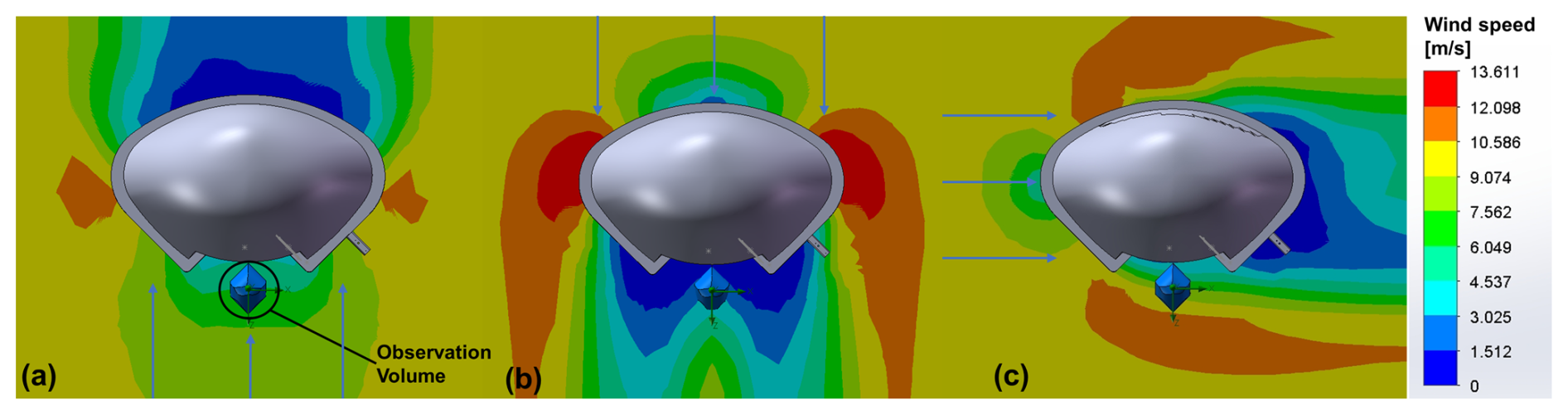
Figure C1 Top view of wind speed distribution in the simulated wind field. The 3D-PPI facing 10 m s⁻¹ wind (a), back facing 10 m s⁻¹ wind (b), and side facing 10 m s⁻¹ wind (c). The color gradient represents wind speed, with the observation volume indicated in panel (a).

When the 3D-PPI is facing the wind (Fig. C1a), the observation volume experiences an average wind speed of approximately 6.0 m s⁻¹. Moreover, turbulence may occur within the observation volume. When the 3D-PPI is back facing the wind (Fig. C1b), the average wind speed in the observation volume is only about 3.5 m s⁻¹, which is obviously due to the shielding of the wind by the instrument. When the 3D-PPI is side facing the wind (Fig. C1c), the observation volume shows an average wind speed of about 8.5 m s⁻¹, exhibiting the smallest difference from 10 m s⁻¹ compared to the other two situations. However, part of the observation volume close to the instrument is still shielded by the housing, which to some extent also affects the representativeness of the wind field, and subsequent consideration will need to be given to improving the instrument design to solve this problem.

In addition to 10 m s⁻¹, we also simulated 5, 20, and 40 m s⁻¹ wind speed fields, and all of them obtained the consistent conclusion that the wind speed in the observation volume is closest to the simulated wind speed when the instrument is side facing the prevailing wind direction. Therefore, the instrument should be installed sideways to the dominant wind direction in the area to minimize the disturbance of the instrument to the natural wind field. The prevailing wind direction in the area is west, so the 3D-PPI is installed facing towards the south.