A comprehensive characterization of empirical parameterizations for OH exposure in the Aerodyne Potential Aerosol Mass Oxidation Flow Reactor (PAM-OFR)

The oxidation flow reactor (OFR) has been widely used to simulate secondary organic aerosol (SOA) formation in laboratory and field studies. OH exposure (OH_exp), representing the extent of hydroxyl (OH) radical oxidation and normally expressed as the product of OH concentration and residence time in the OFR, is important in assessing the oxidation chemistry in SOA formation. Several models have been developed to quantify the OH_exp in OFRs, and empirical equations have been proposed to parameterize OH_exp. Practically, the empirical equations and the associated parameters are derived under atmospheric relevant conditions (i.e., external OH reactivity) with limited variations in calibration conditions, such as residence time, water vapor mixing ratio, and ozone (O₃) concentration. Whether the equations or parameters derived under limited sets of calibration conditions can accurately predict the OH_exp under dynamically changing experimental conditions with large variations (i.e., extremely high external OH reactivity) in real applications remains uncertain. In this study, we conducted 62 sets of experiments (416 data points) under a wide range of experimental conditions to evaluate the scope of the application of the empirical equations to estimate OH_exp. Sensitivity tests were also conducted to obtain a minimum number of data points, which is necessary for generating the fitting parameters. We showed that, for the OFR185 mode (185 nm lamps with internal O₃ generation), except for external OH reactivity, the parameters obtained within a narrow range of calibration conditions can be extended to estimate the OH_exp when the experiments are in wider ranges of conditions. For example, parameters derived within a narrow water vapor mixing ratio range (0.49 %–0.99 %, corresponding to 15.1 %–30.8 % of relative humidity at 101.325 kPa and 298 K) can be extended to estimate the OH_exp under the entire range of water vapor mixing ratios (0.49 %–2.76 %, equivalent to 15.1 %–85.7 % of relative humidity under identical conditions). However, the parameters obtained when the external OH reactivity is below 23 s⁻¹ could not be used to reproduce the OH_exp under the entire range of external OH reactivity (4–204 s⁻¹). For the OFR254 mode (254 nm lamps with external O₃ generation), all parameters obtained within a narrow range of conditions can be used to estimate OH_exp accurately when experimental conditions are extended. Additionally, when using the OFR254 mode, lamp voltages that are too low should be avoided, as they will generally result in large deviations in the estimations of OH_exp from empirical equations. Regardless of whether the OFR185 or OFR254 mode is used, at least 20–30 data points from sulfur dioxide (SO₂) or carbon monoxide (CO) decay with varying conditions are required to fit a set of empirical parameters that can accurately estimate OH_exp. Caution should be exercised to use fitted parameters from low external OH reactivity to high ones, for instance, those from direct emissions such as vehicular exhaust and biomass burning.

1 Introduction

As the most important oxidant in tropospheric chemistry (Ehhalt, 1999), the hydroxyl (OH) radical is vital in oxidizing primary pollutants such as volatile organic compounds (VOCs) and contributes to secondary organic aerosol (SOA) and tropospheric ozone (O₃) formation. The OH radical has daytime concentrations of 10⁵ to 10⁷ molec. cm⁻³, exhibiting daily (Cao et al., 2020; Tan et al., 2017), seasonal (Friedman and Farmer, 2018), and spatial (Cao et al., 2020; Stone et al., 2012) variations. An average daily OH radical concentration of 1.5 × 10⁶ molec. cm⁻³ is widely used to estimate the photochemical age of an air mass (Mao et al., 2009). Typical VOCs have second-order rate constants of 10⁻¹⁵ to 10⁻¹⁰ cm³ molecule⁻¹ s⁻¹ with OH radicals (Atkinson and Arey, 2003; Atkinson et al., 2006), which can be translated to atmospheric lifetimes of hours to approximately 1 year (Seinfeld and Pandis, 2016). This situation poses challenges in laboratory experiments to directly simulating the OH oxidation of VOCs, which is one of the most important chemical processes in the Earth's atmosphere.

Smog chambers (Cocker et al., 2001; Hildebrandt et al., 2009; Wang et al., 2014) and oxidation flow reactors (OFRs) (George et al., 2007; Kang et al., 2007; Lambe et al., 2011) have been widely employed to simulate the oxidation of VOCs and subsequent SOA formation. For example, the Caltech chamber provides oxidation conditions close to the real atmosphere, making it suitable for the study of complex multi-step reactions and low-volatility products. However, each experiment takes several hours to days, and long-duration experiments are prone to background interference. The Toronto Photo-Oxidation Tube (TPOT) focuses on the study of heterogeneous oxidation reactions of aerosols. Its 0.8 L volume makes it portable, but it is prone to uneven residence time distribution (RTD) and significant wall effects. The Potential Aerosol Mass Oxidation Flow Reactor (PAM-OFR) and the Gothenburg Potential Aerosol Mass Oxidation Flow Reactor (Go:PAM-OFR) are often used to study the transformation of gaseous precursors into particles (such as the formation of SOA). The Go:PAM-OFR has a volume of 7.2 L, which is only half that of the PAM-OFR, making it suitable for experiments on mobile platforms. However, its small volume gives it the same disadvantages as the TPOT, and it is equipped with only a single ultraviolet (UV) lamp, which does not allow as wide a range of controllable oxidation levels as the PAM-OFR. The PAM's moderate volume and central flow sampling can reduce wall effects.

These OFRs normally operate with high concentrations of oxidants (e.g., OH radicals), which lead to a significant acceleration of oxidation reactions, often by orders of magnitude. To reconcile the differences in OH concentration and exposure time between ambient and laboratory settings, the oxidation extent, i.e., OH exposure (OH_exp; molec. cm⁻³ s), is normally used to extrapolate laboratory findings to ambient conditions. Despite drawbacks such as possible altered reaction mechanisms, this approach provides a quantitative assessment of the chemistry during OH oxidation in a reasonable time span and achievable detection capability. The OH_exp has a significant impact on the yield and product distribution during VOC oxidation (Cheng et al., 2021, 2024). Accurate measurement or estimation of the OH_exp during laboratory experiments is therefore the key to understanding the oxidation chemistry that can represent the ambient conditions. In this study, we chose to further investigate the PAM-OFR to explore its OH_exp, as it offers moderate conditions in terms of experiment time, deployment complexity, range of oxidation levels, and wall effects.

The Aerodyne Potential Aerosol Mass OFR (PAM-OFR) is one of the most widely used OFRs for studying SOA formation and evolution (Zhang et al., 2024). It can achieve a wide range of atmospheric OH_exp conditions within short residence times on the order of minutes (Kang et al., 2007; Lambe et al., 2011). The PAM-OFR can be operated in a number of modes, depending on (1) the wavelength of the ultraviolet (UV) light source, (2) the concentration of the externally generated O₃ (if any), and (3) the injection of an external precursor to generate NO_x (= NO + NO₂) or other oxidants (e.g., nitrate radical or halogen atoms) upon photolysis. The most widely used methods for OH generation include combined photolysis of O₂ and H₂O at λ = 185 nm plus photolysis of O₃ at λ = 254 nm (OFR185; Reactions R1–R6) or photolysis of externally added O₃ at λ = 254 nm (OFR254; Reactions R5–R6) (Rowe et al., 2020):

$$\begin{array}{}\text{(R1)}& {\displaystyle }{\mathrm{H}}_{\mathrm{2}}\mathrm{O}+h{v}_{\mathrm{185}}\to \mathrm{H}+\mathrm{OH}\text{(R2)}& {\displaystyle }\mathrm{H}+{\mathrm{O}}_{\mathrm{2}}\to {\mathrm{HO}}_{\mathrm{2}}\text{(R3)}& {\displaystyle }{\mathrm{O}}_{\mathrm{2}}+h{v}_{\mathrm{185}}\to \mathrm{2}\mathrm{O}{(}^{\mathrm{3}}\mathrm{P})\text{(R4)}& {\displaystyle }\mathrm{O}{(}^{\mathrm{3}}\mathrm{P})+{\mathrm{O}}_{\mathrm{2}}\to {\mathrm{O}}_{\mathrm{3}}\text{(R5)}& {\displaystyle }{\mathrm{O}}_{\mathrm{3}}+h{v}_{\mathrm{254}}\to {\mathrm{O}}_{\mathrm{2}}+\mathrm{O}{(}^{\mathrm{1}}\mathrm{D})\text{(R6)}& {\displaystyle }\mathrm{O}{(}^{\mathrm{1}}\mathrm{D})+{\mathrm{H}}_{\mathrm{2}}\mathrm{O}\to \mathrm{2}\mathrm{OH}.\end{array}$$

To obtain the OH_exp under these two modes in the PAM-OFR, one can perform decay experiments on trace gases, such as sulfur dioxide (SO₂) and carbon monoxide (CO), and fit the OH_exp based on known second-order rate constants between the OH radical and the trace gases, defined as OH_exp, dec. Based on the results of the decay experiments, Li et al. (2015) and Peng et al. (2015) developed estimation equations to parameterize OH_exp as a function of easily measurable quantities, which is denoted as OH_exp, est. A set of parameters (a–f and x–z, respectively) for the estimation equations of the OFR185 and OFR254 modes (see Sect. 2.3 for details) was obtained by fitting the estimation equations to OH_exp, dec values obtained from decay experiments.

When using the PAM-OFR in field studies, it is necessary to obtain concurrent OH_exp that is representative of the ambient conditions. However, environmental conditions in field studies (e.g., humidity, temperature) are constantly changing, making it challenging to replicate these conditions for OH_exp estimation. In some field studies using the PAM-OFR, concurrent OH_exp was estimated by measuring the relative decay of benzene and toluene (Liao et al., 2021; Liu et al., 2018). Additionally, some studies have mentioned that OH concentrations can be indirectly measured by detecting the decay of tracers such as 3-pentanol, 3-pentanone, pinonaldehyde, or butanol-d9 (Barmet et al., 2012). However, the measurement of all these organic tracers requires specific, sophisticated instruments such as proton-transfer-reaction time-of-flight mass spectrometers (PTR-TOF-MSs). Additionally, switching the instrument back and forth between the front and end of the OFR during field measurements can result in some loss of real-time VOC data before entering the OFR. To obtain accurate OH_exp, some studies explicitly modeled the radical chemistry in the PAM-OFR (Li et al., 2015; Ono et al., 2014; Peng et al., 2015). The estimation equations developed by Li et al. (2015) and Peng et al. (2015), although empirical, reproduced the OH_exp from models within 10 %, making them a good choice because these equations only require the input of a few easily available parameters. However, it is unclear whether the fitted parameters obtained under certain conditions can still accurately estimate OH_exp when experimental conditions, such as UV light intensity, water vapor mixing ratio, residence time, and external OH reactivity (OHR_ext), undergo significant changes. Furthermore, there is currently no consensus on the minimum number of decay experiments required to obtain accurate parameterization for OH_exp estimation using these equations. This facet is important for field studies using the PAM-OFR where only limited numbers of decay experiments can be performed to obtain concurrent OH_exp estimation.

In this study, we conduct a series of experiments using the decay of SO₂ and CO to estimate the OH_exp in the PAM-OFR under the OFR185 and OFR254 modes. The applicability of previously developed OH_exp estimation equations to obtain accurate OH_exp in the PAM-OFR is evaluated by linear regression of OH_exp, est against OH_exp, dec. We also evaluate how well estimation equations perform when using limited ranges of experimental parameters (e.g., OHR_ext, residence time, water mixing ratio) or different trace gases (SO₂ and CO) and provide recommendations. In addition, we propose the minimal number of trace gas decay experiments required to obtain a set of usable parameters for the OH_exp estimation equations. Finally, we also compare the advantages and disadvantages of the OFR185 and the OFR254 modes from the perspective of the quantification of OH_exp. The methodology of this study can be applied to laboratory and field experiments for OH_exp estimation using the PAM-OFR or other OFRs that follow a plug flow assumption.

2 Methods

2.1 The PAM-OFR

Experiments were conducted using an Aerodyne PAM-OFR (Aerodyne Research Inc., Billerica, MA, US), which is a horizontal aluminum cylindrical chamber with an internal volume of 13.3 L. The PAM-OFR operates in continuous-flow mode. Four low-pressure Hg lamps are installed inside the reactor to produce UV light with characteristic spectral lines (e.g., 185 and 254 nm). The OH is generated via OFR185 using two ozone-producing Hg lamps (GPH436T5VH/4P, Light Sources, Inc.) or via OFR254 using two ozone-free Hg lamps (GPH436T5L/4P, Light Sources, Inc.) to photolyze externally added ozone. A flow of nitrogen purge gas, ranging from 0.2 to 0.3 L min⁻¹, is introduced between the lamps and sleeves. This nitrogen gas flow serves to reduce the heat generated by the lamps and prevent the formation and accumulation of ozone between the lamps and the quartz tubes that isolate them from the sample flow in the OFR. A fluorescent dimming ballast is used to control the photon flux by regulating the voltage applied to the lamps, which allows us to generate different OH concentrations. In typical measurement sequences, nine lamp voltage settings (including lights off) were cycled through every 2–3 h. The dimming voltage ranged from 0 to 10 V direct current (DC).

2.2 OH_exp estimation through decay of SO₂ and CO (OH_exp, dec)

OH_exp can be indirectly measured by detecting the decay of the tracers with known reaction rates. Inorganic trace gases (SO₂ or CO) react with OH radicals at slower rates compared to most VOCs. However, considering the complex oxidation chemistry of VOCs, SO₂ and CO can better capture the features of real OHR_ext decay and effective OHR_ext (Peng et al., 2015). We performed systematic decay experiments with SO₂ and CO in the PAM-OFR, with conditions tabulated in Tables S1 and S2 in the Supplement. Figure S1 shows the schematics of the experimental setups in the OFR185 and OFR254 modes. In the OFR185 mode, the injected gas flow at the inlet of the PAM is made up of three sub-flows: (1) the trace gas flow, i.e., SO₂ of 0.2–8.7 ppm or CO of 10.2–207.5 ppm supplied from gas cylinders (purity: 99.9 % of SO₂, 99.95 % of CO; Shanghai Shenkai Gases Technology CO., LTD.); (2) dry clean air from a zero-air generator (ZAS-100/150, Convenient) with a non-methane hydrocarbon content of less than 1 ppb; and (3) the humidified clean air passed through a Nafion humidifier (FC100-80-6MSS, Perma Pure). By adjusting the ratio of dry air to humidified air, the water vapor mixing ratio in the PAM-OFR can be controlled. Additionally, they also serve as makeup flows to maintain a constant flow rate. At the outlet of the reactor, the gas flow was sampled from an internal perforated Teflon ring. The gas-phase species (O₃, SO₂, and CO) were detected using an ultraviolet ozone analyzer (UV-100, Eco Sensors), an SO₂ monitor (Model 43i, Thermo Scientific), and a CO monitor (G2401, Picarro), respectively. In the OFR254 mode, in addition to the previously mentioned setup, externally generated O₃ (through UV photolysis) with desired concentrations was injected at the inlet of the PAM-OFR.

Figure S2a and b depict examples of set and measured parameters during experiments conducted in the OFR185 and OFR254 modes, respectively. In the OFR185 mode, without radical generation to oxidize the tracer species, their concentration was allowed to stabilize under dark conditions. Once the concentration reached a steady state, the UV lamps were turned on. Different light intensities lead to varying levels of decay of SO₂ or CO after oxidation, reflecting different OH_exp within the PAM-OFR. In the OFR254 mode, it is necessary to obtain the initial concentration of O₃ injected into the PAM-OFR in the absence of OHR_ext. While the SO₂ or CO concentration was in the process of stabilizing, the O₃ flow was temporarily blocked outside the PAM-OFR using a valve. Dry clean air was then introduced to compensate for this portion of the flow, ensuring a constant total flow throughout the entire process. Once the tracer species concentration had reached a steady state, the O₃ was then allowed to flow into the PAM-OFR. The total OH_exp, dec in the reactor was varied over a wide range (approximately 10⁹–10¹² molec. cm⁻³ s) by changing the UV light intensity, water mixing ratio, and residence time. The mean residence time was obtained from the ratio of the internal volume of and the total flow rate through the PAM-OFR. In the calculation of OH_exp, dec (see the paragraph below), plug flow conditions were assumed, and this has been shown by Li et al. (2015) and Peng et al. (2015) to agree with the RTD approach for OH_exp when using species (such as SO₂ or CO) with low reaction rate constants with OH radicals (k_i, OH).

OH_exp, dec in the PAM-OFR was calculated from the pseudo-first-order reaction of OH with SO₂ or CO, whose k_i, OH values have been well characterized ($k_{{\mathrm{SO}}_{\mathrm{2}},\mathrm{OH}}$ = 9.49 × 10⁻¹³ cm³ molec.⁻¹ s⁻¹ and k_CO, OH = 2.4 × 10⁻¹³ cm³ molec.⁻¹ s⁻¹ at 1 atm and 298 K) (Burkholder et al., 2020; Cao et al., 2020). By measuring the decay of SO₂ or CO, the corresponding OH_exp, dec is calculated as follows:

$$\begin{array}{}\text{(1)}& {\mathrm{OH}}_{\exp ,\mathrm{dec}}={\displaystyle \frac{-\mathrm{1}}{k_{i,\mathrm{OH}}}}\times \ln \left({\displaystyle \frac{C_{i,\mathrm{out}}}{C_{i,\mathrm{in}}}}\right),\end{array}$$

where C_i,in is the concentration of reactant i injected into the PAM-OFR (ppb), C_i,out is the reactant i concentration at the PAM-OFR outlet (ppb), and k_i,OH is the second-order rate constant between the trace species (SO₂ or CO) and OH radicals.

Despite the use of nitrogen as a purge gas to reduce the heat generated by the lamp, temperature variations were still observed within the PAM-OFR. There was a maximum deviation of approximately 13 °C from 25 °C when using SO₂ as the OHR source. However, the $k_{{\mathrm{SO}}_{\mathrm{2}},\mathrm{OH}}$ was 8.85 × 10⁻¹³ cm³ molec.⁻¹ s⁻¹ at 38 °C (Burkholder et al., 2020), which results in the calculated OH_exp, dec being only approximately 7 % higher than that derived from $k_{{\mathrm{SO}}_{\mathrm{2}},\mathrm{OH}}$ at 25 °C. Pan et al. (2024) noted that temperature increases caused by lamp heating exerted minimal influence on gas-phase reaction rates, with SO₂ decay and OH exposure showing negligible variations. Therefore, the influence of temperature on reaction kinetics was not considered in this study.

2.3 OH_exp estimation from empirical equations (OH_exp, est)

Li et al. (2015) proposed an OH_exp, est estimation equation (Eq. 2) for OFR185 based on easily measurable quantities:

$$\begin{array}{}\text{(2)}& \begin{array}{rl}& {\mathrm{OH}}_{\exp ,\mathrm{est}}=\\ & {\mathrm{10}}^{\left[\begin{array}{c}a+\left(b+c\times {\mathrm{OHR}}_{\mathrm{ext}}^d+e\times \log \left({\mathrm{O}}_{\mathrm{3},\mathrm{out}}\times \frac{\mathrm{180}}{t}\right)\times {\mathrm{OHR}}_{\mathrm{ext}}^f\right)\\ \times \log \left({\mathrm{O}}_{\mathrm{3},\mathrm{out}}\times \frac{\mathrm{180}}{t}\right)+\log {\mathrm{H}}_{\mathrm{2}}\mathrm{O}+\log \left(\frac{t}{\mathrm{180}}\right)\end{array}\right]},\end{array}\end{array}$$

where a–f are fitting parameters (values are reported in Table S5); O_3, out is the ozone concentration measured at the exit of the PAM-OFR (molec. cm⁻³), which serves as a surrogate for UV flux; H₂O is the water vapor mixing ratio in the PAM-OFR (%), which is influenced by both temperature and relative humidity; and t is mean residence time (s). The total external OH reactivity is represented by OHR_ext (s⁻¹) = ∑_ik_i[C_i], where k_i and [C_i] are the rate constants with OH and the concentration of the OH-consuming reactant i in the system (Wang et al., 2020).

Peng et al. (2015) proposed another equation (Eq. 3) for OH_exp, est in OFR254:

$$\begin{array}{}\text{(3)}& {\mathrm{OH}}_{\exp ,\mathrm{est}}={\mathrm{10}}^{\left[x+\log \left(-\log r_{{\mathrm{O}}_{\mathrm{3}}}\right)+y\times {\left(\frac{{\mathrm{OHR}}_{\mathrm{ext}}}{{\mathrm{O}}_{\mathrm{3},\mathrm{in}}}\right)}^z\right]},\end{array}$$

where x–z are fitting parameters (values are reported in Table S6); $\log r_{{\mathrm{O}}_{\mathrm{3}}}\left(\log \right({\mathrm{O}}_{\mathrm{3},\mathrm{out}}/{\mathrm{O}}_{\mathrm{3},\mathrm{in}}\left)\right)$ is the logarithm of the ratio between the output and input O₃ concentrations, which serves as a surrogate for UV flux and also captures the effect of H₂O; and O_3, in is the concentration of externally injected O₃ into the PAM-OFR (molecules cm⁻³).

In total, we performed 62 sets of trace gas decay experiments with 416 data points for the OH_exp, dec, with 25 sets and 175 data points in the OFR185 mode and 37 sets and 241 data points in the OFR254 mode. In the OFR185 mode, the 175 experiments cover an OH_exp, dec range of 3.57 × 10⁸–5.52 × 10¹² molec. cm⁻³ s, with an equivalent photochemical age ranging from 4 min to 43 d. In the OFR254 mode, the 241 experiments cover an OH_exp, dec range of 1.01  × 10⁹–2.18 × 10¹² molec. cm⁻³ s, with an equivalent photochemical age ranging from 11 min to 17 d. The error in OH_exp, dec is derived from the measurement error of the tracer gas, propagated through Eq. (1). When OH_exp, dec ranged from 3.6 × 10⁸–5.5 × 10¹² molec. cm⁻³ s, the resulting error values were 1.9 × 10⁸–2.4 × 10¹⁰ molec. cm⁻³ s.

After obtaining the OH_exp, dec values, we used Eqs. (2) and (3) to fit the parameters a–f and x–z for the OFR185 and OFR254 modes, respectively, given that the experimental parameters, such as OHR_ext, O_3, out, H₂O, and t (in Eq. 2) as well as $r_{{\mathrm{O}}_{\mathrm{3}}}$, OHR_ext, and O_3, in (in Eq. 3), are known. The OH_exp, est values were then reconstructed with the fitted parameters and the experimental parameters and were compared with the OH_exp, dec values via linear regression analysis. Similarly, the error values for all OH_exp, est values are at least 1 order of magnitude smaller than the respective OH_exp, est values. The generation of OH radicals in the PAM-OFR is related to the photon fluxes at λ = 185 nm (I₁₈₅) and λ = 254 nm (I₂₅₄). According to Rowe et al. (2020), I₁₈₅:I₂₅₄ is specific to the Hg lamp utilized. Since the OH_exp estimation equation for OFR185 uses O₃ concentration as a measurable surrogate for the UV flux at 185 nm, it is also lamp-specific. Because the UV lamps used in our study are different from the BHK lamps employed by Li et al. (2015), we anticipate that the parameters a–f fitted from our decay experiments (Table S5) should be quite different from those in Li et al. (2015), which is indeed the case. Similarly, fitting parameters x–z for the OFR254 mode from our decay experiments (Table S6) are also different from those in Peng et al. (2015).

3 Results and discussion

3.1 The OFR185 mode: OHR_ext level relevant to ambient conditions

Field studies showed that the environmental OHR_ext mainly fluctuated between 10–30 s⁻¹ (Fuchs et al., 2017; Lou et al., 2010; Lu et al., 2010; Tan et al., 2018; Yang et al., 2017). To investigate the factors that potentially affect the fitting parameters of Eq. (2) in the estimation of OH_exp under ambient conditions, we first performed 16 sets of experiments with OHR_ext of 4–23 s⁻¹ using SO₂ as the OHR_ext source. With the measured OH_exp, dec, the parameters (a–f) were first derived, which were used to reconstruct OH_exp, est using Eq. (2) with known OHR_ext, ozone concentration (O_3, out), water vapor mixing ratio (H₂O), and residence time (t). The reconstructed OH_exp, est values were plotted against the OH_exp, dec values calculated from the trace gas decay experiments, as shown in Fig. 1. The 1 : 2 and 2 : 1 lines indicate a difference of approximately 0.5 orders of magnitude between OH_exp, dec and OH_exp, est, which is considered to be acceptable as an uncertainty in OH_exp estimation.

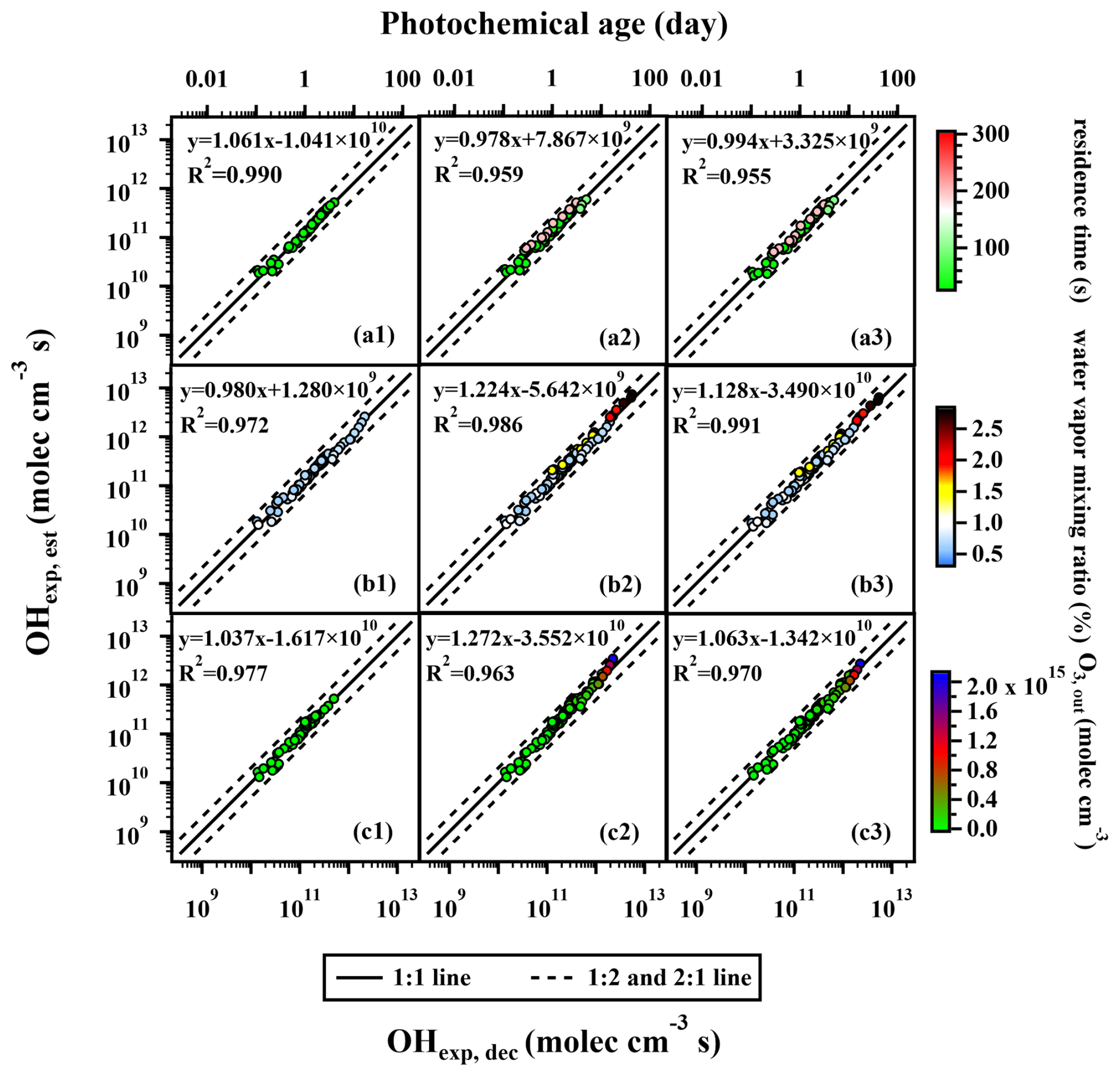
Figure 1 The regression results of OH_exp, est and OH_exp, dec when variations occurred in the (a1–a3) residence time, (b1–b3) water vapor mixing ratio, and (c1–c3) output O₃ concentration under atmospheric relevant OHR_ext levels (4–23 s⁻¹). Compared to panels (a1), (b1), and (c1), panels (a2), (b2), and (c2) incorporated additional data points with higher t, H₂O, and O_3, out values, respectively, but still utilized the fitting parameters FP_st, 185, FP${}_{{\mathrm{lH}}_{\mathrm{2}}\mathrm{O},\mathrm{185}}$, and FP${}_{{\mathrm{lO}}_{\mathrm{3}},\mathrm{185}}$ obtained from the lower condition range to estimate OH_exp, est. In panels (a3), (b3), and (c3), all data points within the extended condition range were used to refit the parameters a–f, and the resulting FP_et, 185, FP_eH2O, 185, and FP_eO3, 185 were employed to estimate OH_exp, est (s: short; l: low; e: extended). All the error values for OH_exp, dec are 0.5 or even 2 orders of magnitude smaller than the corresponding OH_exp, dec values. When applying a logarithmic scale, the error bars become difficult to represent. To enhance the readability of the graph, error bars are not included. For the same reason, error bars for OH_exp, est values are also not displayed.

Firstly, we investigated the effect of changing residence time on the OH_exp estimation. With other experimental parameters (i.e., H₂O, O_3, out, and OHR_ext) being similar, we set the residence time to a low value (33 s) and also a range of higher values (61–200 s). The detailed ranges of each experimental condition for different datasets are listed in Table S3. With the residence time of 33 s, the reconstructed OH_exp, est correlates well with the experimental OH_exp, dec (slope = 1.061 and R² = 0.990; Fig. 1a1). The set of fitted parameters a–f (FP_st, 185; st: short time) applied in Fig. 1a1 is presented in Table S5. When the residence time was increased to 61–200 s, the interpolated OH_exp, est utilizing FP_st, 185 was also in good correlation with OH_exp, dec (slope = 0.978, R² = 0.959; Fig. 1a2). We also derived fitted parameters (FP_et, 185; et: extended t) using the data points with the extended range of residence time (33–200 s). Not surprisingly, with the application of FP_et, 185, OH_exp, est also correlated well with OH_exp, dec (slope  = 0.994, R² = 0.955; Fig. 1a3). The results indicate that variation in residence time does not significantly affect the fitting parameters of Eq. (2) for the OH_exp estimation. From an experimental perspective, since OH_exp is the product of OH radical concentration ([OH]) and the residence time (t), as long as the change in t does not significantly alter the quasi-steady-state [OH], the fitted parameters from a narrow range of t should be applicable to situations of longer t. Mathematically, two terms of $\mathrm{180}/t$ and $t/\mathrm{180}$ are related to t, ranging from 0.90–5.45 and 0.18–1.11, respectively, which do not contribute significantly to the exponent in Eq. (2) after taking the logarithm of them. It is important to note that the above discussion regarding residence time assumes plug flow conditions within the PAM-OFR, which are applicable to substances with low k_i, OH, such as SO₂ (or CO). For species that react rapidly with OH, such as monoterpenes or toluene, localized concentration gradients can develop within the OFR, leading to a significant uneven actual RTD that affects the estimation of OH_exp (Palm et al., 2018).

Similarly, we then investigated the impacts of H₂O on the estimation of OH_exp. Applying fitted parameters from experiments of low water vapor mixing ratios (0.49 %–0.99 %; Fig. 1b1) (FP${}_{{\mathrm{lH}}_{\mathrm{2}}\mathrm{O},\mathrm{185}}$; lH₂O: low H₂O) to data spanning a wide range of water vapor mixing ratios (0.49 %–2.76 %) also yielded a reasonably good correlation between OH_exp, est and OH_exp, dec (Fig. 1b2). This could be attributed to the fact that the term logH₂O in Eq. (2) does not contribute significantly to the exponent.

As for ozone concentration, applying fitting parameters (FP${}_{{\mathrm{lO}}_{\mathrm{3}},\mathrm{185}}$; lO₃: low O_3, out) from experiments of low ozone concentration (1.44 × 10¹²–6.79 × 10¹³ molec. cm⁻³, Fig. 1c1) to reconstruct the data for a wide range (1.44 × 10¹²–2.03 × 10¹⁵ molec. cm⁻³) yielded a reasonably good correlation between OH_exp, est and OH_exp, dec (Fig. 1c2). It only resulted in a mildly increased slope (from 1.063 to 1.272) and similar R² values (both are 0.970) as compared to those using the whole ozone concentration range (Fig. 1c3).

Ideally, trace gas decay experiments covering the entire ranges of the t, H₂O, and O_3, out variations under real experimental conditions should be conducted, which is labor-intensive. Practically, due to the atmospherically relevant variations that occur in t, H₂O, and O_3, out during the real experiments, the ranges of t, H₂O, and O_3, out covered by trace gas decay experiments are usually narrower compared to the real experiments. Our results suggest that the fitting parameters (a–f) obtained from calibration experiments with relatively narrow ranges of t, H₂O, and O_3, out can still provide a reliable estimation of OH radical levels during the real experiments, which would cover wider ranges of these conditions.

It is noteworthy that reliable estimations can be achieved regardless of whether the narrow range is situated within the lower or higher interval of the full condition range. Figure 1 demonstrated the case where the narrow range was situated within the lower interval, while Fig. S3 presented the case where the narrow range was situated within the higher interval. The detailed ranges of each experimental condition for different datasets are listed in Table S3. As shown in Fig. S3, the data points in Fig. S3a1 had residence times of 100–296 s, the data points in Fig. S3b1 had water vapor mixing ratios of 1.04 %–2.76 %, and the data points in Fig. S3c1​​​​​​​ had O_3, out of 8.45 × 10¹³–2.03 × 10¹⁵ molec. cm⁻³. Figure S3a2, b2, and c2 built on Fig. S3a1, b1, and c1 by incorporating data points with shorter t (33–61 s), lower H₂O (0.49 %–0.97 %), and lower O_3, out (1.44 × 10¹²–6.79 × 10¹³ molec. cm⁻³), respectively, but still used fitting parameters a–f obtained from the higher range of conditions to estimate OH_exp, est. In Fig. S31a3, b3, and c3, the parameters a–f were refitted using all the data points included in the expanded t, H₂O, and O_3, out ranges, respectively, and the obtained a–f were used to estimate OH_exp, est. Using Fig. S3a1–a3 as an example, the slope and R² values in Fig. S3a2 and a3 were very close to 1, reflecting the good consistency between OH_exp, est and OH_exp, dec. In the OFR254 mode discussed later (Fig. 4c1–c3), this narrower range can also be situated within the middle interval of the full condition range. This applicability of fitting parameters obtained from narrow ranges of experimental conditions is beneficial for quickly obtaining concurrent OH_exp during the experiments in field measurements.

3.2 The OFR185 mode: OHR_ext level relevant to emission sources

The experimental conditions in the PAM-OFR often involve not only general atmospheric conditions (OHR_ext < 30 s⁻¹) but also high-concentration conditions, e.g., those directly from emission sources. For instance, the OHR_ext of direct vehicle emission can be as high as 1000 s⁻¹, with plenty of reducing gases such as CO and VOCs (Nakashima et al., 2010). To evaluate the applicability of Eq. (2) under situations of high OHR_ext, we performed high OHR_ext (up to 204 s⁻¹) experiments using high concentrations of SO₂ as the OHR_ext source. Compared to the data points shown in Fig. 2a (4–23 s⁻¹), Fig. 2b and c included additional data points with higher OHR_ext values (198–204 s⁻¹), while the other conditions remained similar. In Fig. 2b, the parameters a–f (FP_lOHR, 185; lOHR: low OHR_ext) obtained from the low OHR_ext data points were used to estimate OH_exp, est, yet those used in Fig. 2c were refitted from the data points with extended OHR_ext range (4–204 s⁻¹). It could be observed from Fig. 2b that, when estimating OH_exp using FP_lOHR, 185, OH_exp, est values of the high OHR_ext data points were significantly overestimated, with a difference of more than 2 orders of magnitude compared to OH_exp, dec. This observation suggests that, differently to cases for the residence time, water vapor mixing ratio, and ozone concentration shown in the section above, FP_lOHR, 185 values were not applicable to high OHR_ext conditions.

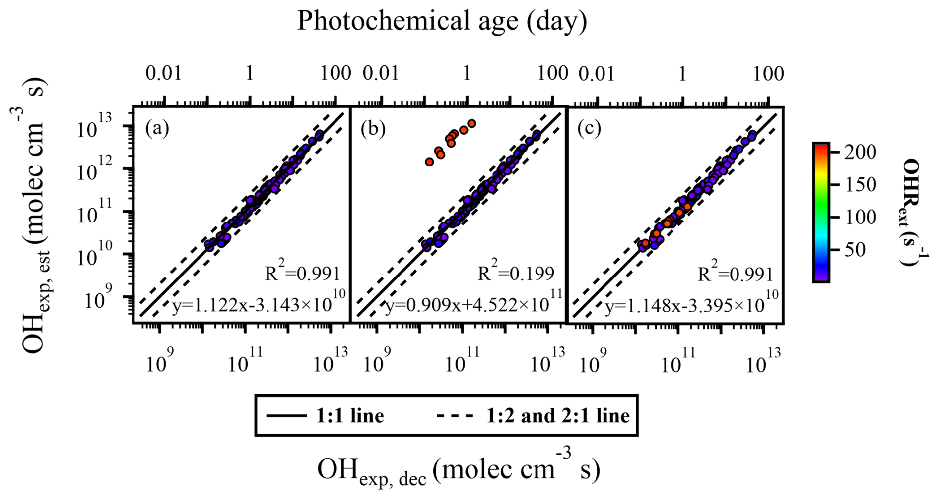
Figure 2 The regression results of OH_exp, est and OH_exp, dec with different OHR_ext levels. In panel (a), data points with atmospheric relevant OHR_ext levels (4–22 s⁻¹) were applied. In addition to the data points contained within panel (a), panel (b) included additional data points with OHR_ext levels related to emission sources (198–204 s⁻¹), but FP_lOHR, 185 values were still used to estimate OH_exp, est. In panel (b), data points in red show that the OH_exp, est values of these high OHR_ext data points were significantly overestimated. FP_lOHR, 185 values were not applicable to high OHR_ext conditions. The data points in panel (c) were identical to those in panel (b), but the estimation of OH_exp, est utilized the FP_eOHR, 185 obtained by fitting all data points across the full range of OHR_ext levels.

We then investigated the possible causes of the discrepancy for OH_exp estimation between FP_lOHR, 185 and FP_eOHR, 185 (eOHR: extended OHR_ext). From a mathematical perspective, according to Eq. (2), the third term c × OHR${}_{\mathrm{ext}}^d$ × log(O${}_{\mathrm{3},\mathrm{out}}\times \mathrm{180}/t$) and the fourth term e × OHR${}_{\mathrm{ext}}^f\times \left[\log \right({\mathrm{O}}_{\mathrm{3},\mathrm{out}}\times \mathrm{180}/t){]}^{\mathrm{2}}$ are associated with OHR_ext and involve fitted parameters of c–f. To investigate their relationships with OHR_ext, we performed a sensitivity test with a fixed ozone concentration (1.77 × 10¹⁴ molec. cm⁻³) and residence time (89 s), which were mean values during our experiments. When using the c–f values of FP_lOHR, 185 (−0.13922, 0.26786, 0.0026332, and 0.4917), the variations in the third term, the fourth term, and their sum with respect to OHR_ext are shown in Fig. S4a1–a3, respectively. The third term (Fig. S4a1) was negative and decreased as OHR_ext increased, while the fourth term (Fig. S4a2) was positive and increased as OHR_ext increased. The sum of them (Fig. S4a3), however, firstly decreased and then started to increase at approximately OHR_ext = 21 s⁻¹, possibly owing to a slower decrease in the third term or a faster increase in the fourth. If contributions from other terms in Eq. (2) were constant, this led to an increase in OH_exp as OHR_ext increased beyond 21 s⁻¹. Our results showed that the expectation that OH_exp should decrease with increasing OHR_ext (Li et al., 2015) was applicable to the lower ranges of OHR_ext, i.e., under atmospheric relevant conditions. With a further increase in OHR_ext, i.e., above atmospheric relevant condition, the fitted parameters obtained from the dataset with FP_lOHR, 185 were not applicable.

When using the c–f values of FP_eOHR, 185 (−0.079114, 0.36805, 0.0041654, and 0.38722), the trends of the third and the fourth terms (Fig. S4b1 and b2, respectively) were similar to those with low OHR_ext (Fig. S4a1 and a2, respectively); their sum, however, gave a monotonically decreasing trend as OHR_ext increased (Fig. S4b3), consistent with the expectation that OH_exp should decrease with increasing OHR_ext (Li et al., 2015). The curve in Fig. S4b3 can continue to decrease monotonically at higher OHR_ext values, at least until 2000 s⁻¹.

From the perspective of oxidation chemistry, high concentrations of gas-phase SO₂ could lead to more SO₂ entering the particle phase. The H₂O₂ in the liquid water of nucleated sulfuric acid aerosols would further oxidize SO₂ (Liu et al., 2020), which could lead to the discrepancy for OH estimation between low OHR and extended high OHR.

Nevertheless, the good agreement between OH_exp, est and OH_exp, dec in Fig. 2c (using refitted parameters from the dataset of extended OHR_ext) indicates that Eq. (2) can still be used to estimate OH_exp under high OHR_ext conditions. This conclusion is further supported by the results of OH_exp obtained using CO as the OHR_ext source (see Fig. 3 and the subsection below) under extremely high OHR_ext conditions (up to 1200 s⁻¹). This is advantageous for the use of the PAM-OFR in simulations of SOA formation from direct emission sources (e.g., vehicular exhaust and biomass burning) where OHR_ext is extremely high. It is, however, desirable to have OH_exp estimated under similarly high OHR_ext for those experiments to accurately represent the extent of oxidation.

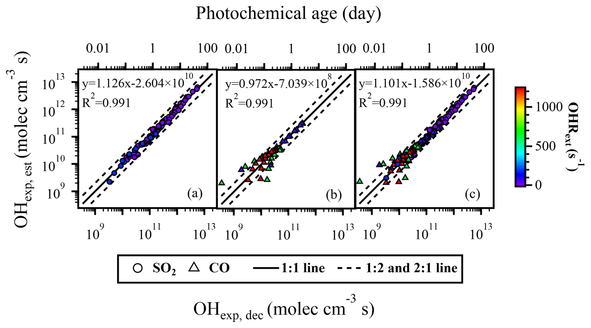
Figure 3 The regression results of OH_exp, dec and OH_exp, est in the OFR185 mode with (a) SO₂ and (b) CO as OHR_ext sources. (c) Results from all experiments (using SO₂ and CO) in the OFR185 mode.

3.3 The OFR185 mode: SO₂ and CO as OHR_ext sources

Peng et al. (2015) suggested that SO₂ can better capture the features of real OHR_ext decay and effective OHR_ext. The reaction between SO₂ and OH is relatively straightforward and is not expected to undergo too many side reactions. CO is a typical gaseous inorganic compound emitted during combustion process. Using CO as an OHR_ext source to explore the estimation of OH_exp in the simulation of oxidation chemistry for emission sources (i.e., high OHR_ext level) is representative. Therefore, we compared the results with SO₂ (Fig. 3a) and CO (Fig. 3b) as the OHR_ext source. When using SO₂ as the OHR_ext source, all data points agreed within a factor of 2 (Fig. 3a), while only approximately 83 % of the data points agreed within a factor of 2 when CO was used as the OHR_ext source (Fig. 3b). The deviating data points were mostly concentrated in areas with high OHR_ext (> 600 s⁻¹) and low O_3, out concentration (10¹²–10¹³ molec. cm⁻³), where the removal of CO was relatively low. Li et al. (2015) observed increased deviations between OH_exp, est and OH_exp, dec, which were attributed, at least in part, to the increased measurement uncertainties for CO when the decrease in its concentration was marginal. We believe that measurement uncertainty might not be the main reason in our case because most of the decreases in CO concentration during our experiments were larger than the precision of the Picarro G2401 Analyzer (∼ 1.5 ppb at 5 min time resolution). Another possible reason is that, in addition to the reaction with OH radicals, CO may react with some other oxidants, leading to its consumption, while SO₂ was less affected, thereby resulting in more scattered data points for CO. The reaction rate of CO with HO₂ is very slow and is unlikely to play a significant role ($k_{\mathrm{CO},{\mathrm{HO}}_{\mathrm{2}}}$ = 5.55 × 10⁻²⁷ cm³ molec.⁻¹ s⁻¹ at 300 K) (You et al., 2007). Cohen and Heicklen (1972) suggested that CO could also react with atomic oxygen (O(¹D)). Clerc and Barat (1967) reported some appreciable rate coefficients (10⁻¹¹ to 10⁻¹² cm³ molec.⁻¹ s⁻¹) for the reaction between CO and O(¹D), which are higher than those for the reactions of CO with OH (k_CO, OH = 2.4 × 10⁻¹³ cm³ molec.⁻¹ s⁻¹ at 298 K) (Burkholder et al., 2020). It is therefore possible that reaction between CO and O(¹D) might have complicated the decay of CO in the PAM-OFR. To further investigate this aspect, we used the KinSim, a kinetic simulator, to calculate the average mixing ratios of OH, O(¹D), and HO₂ under the specific conditions in the PAM-OFR and then assessed the relative importance of the reactions CO + OH → CO₂ + H, CO + O(¹D) → CO₂, and CO + HO₂ → CO₂ + OH (Li et al., 2015; Peng and Jimenez, 2019, 2020). The results show that, although the reaction rate constant of CO and O(¹D) is 1–2 orders of magnitude higher than that of CO and OH, the concentration of OH is about 6–7 orders of magnitude higher than the concentration of O(¹D), indicating that the reaction of CO with O(¹D) will not have a significant impact on the consumption of CO. The real reason for the scattered data points when using CO in the trace gas decay experiment is still unknown.

Figure 3c includes the results of trace gas decay experiments using both SO₂ and CO as the OHR_ext source. Despite having different reaction rates with OH radicals, the data points could be collectively utilized to fit the parameters for the estimation equation. With approximately 95 % of the results agreeing within a factor of 2, OH_exp, est obtained using the fitted parameters exhibited good agreements (slope = 1.101, R² = 0.991) with OH_exp, dec. Our results thus suggest that, although using CO as the OHR_ext might result in some scattered data points, it was still feasible to use Eq. (2) to estimate OH_exp given that experiments were not performed solely in conditions with high OHR_ext (i.e., high CO concentrations) and low O₃ concentrations. Another benefit of using CO as the OHR_ext source for the estimation of OH_exp is that it introduces complexity in the precursor, which resembled that in real applications. Although not tested in this study, we also note that further trace gas decay experiments in the presence of N₂O $/$ NO_x (typical urban environment) should be conducted when oxidation chemistry in the presence of NO_x is studied (Cheng et al., 2021).

3.4 The OFR254 mode

The equation for OH_exp estimation in the OFR254 mode is simpler compared to that of the OFR185 mode. According to Eq. (3), under the OFR254 mode, the three parameters potentially affecting the OH_exp are OHR_ext, input O₃ concentration, and $r_{{\mathrm{O}}_{\mathrm{3}}}$. The detailed ranges of each experimental condition for different datasets are listed in Table S4. We found that, compared to Fig. 1, the data points in Fig. 4 were more scattered. Most of the R² values in Fig. 4 were below 0.9, indicating that, when using SO₂ as the OHR_ext source, the estimation of OH_exp (using Eq. 3) under the OFR254 mode did not perform as well as that under the OFR185 mode (using Eq. 2). Firstly, we investigated the impacts of OHR_ext. Figure 4a1 showed the regression results of OH_exp, est and OH_exp, dec when OHR_ext ranged from 5 to 14 s⁻¹. The parameters x–z (FP_lOHR, 254; lOHR: low external OHR) (Table S6) were obtained by fitting Eq. (3) to OH_exp, dec. In Fig. 4a2, the same set of fitted parameters FP_lOHR, 254 from Fig. 4a1 was used for a wider range of OHR_ext (5–21 s⁻¹). From the regression results (slopes of 1.050 and 1.024, R² of 0.890 and 0.894), the same set of parameters yielded similar estimation performance for OH_exp despite a wider range of OHR_ext in Fig. 4a2 compared to that of Fig. 4a1. At the same time, these results were not much different from those (slope = 1.071, R² = 0.891) using a refitted set of parameters (FP_eOHR, 254; eOHR: extended external OHR) for the wider range of OHR_ext (Fig. 4a3). Even though the correlation was not as good as that in the OFR185 mode, approximately 85 % of the data points agreed within a factor of 2. We did not further extend the OHR_ext to values as high as those in the OFR185 mode as discussed above, since the OFR254 mode was much less oxidative and might not be as suitable for simulating the oxidation chemistry of extremely high OHR_ext as that from direct emissions.

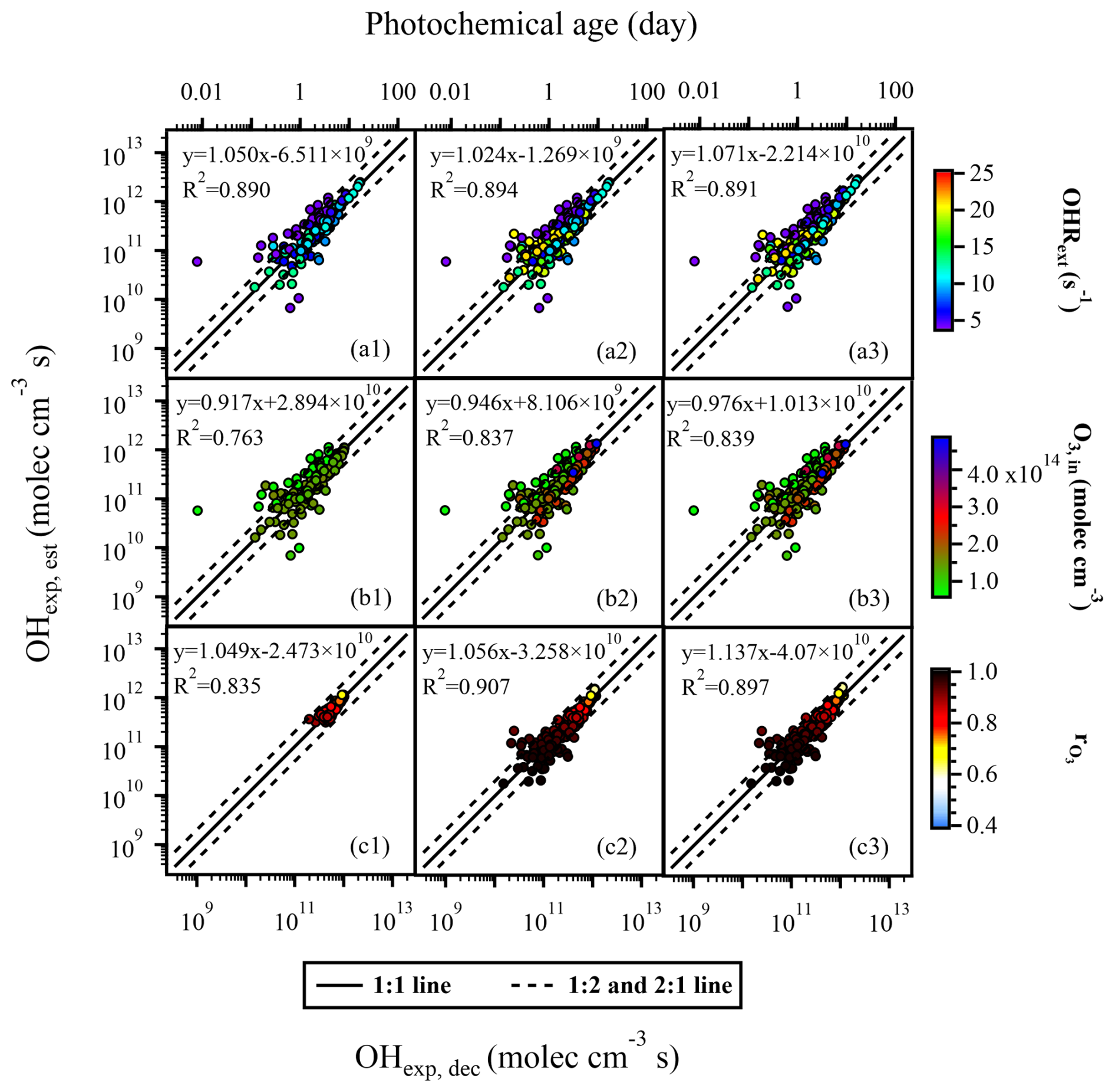
Figure 4 The regression results of OH_exp, est and OH_exp, dec when variations occurred in (a1–a3) OHR_ext, (b1–b3) input O₃ concentration, and (c1–c3) $r_{{\mathrm{O}}_{\mathrm{3}}}$. Compared to panels (a1), (b1), and (c1), panels (a2), (b2), and (c2) incorporated additional data points with extended OHR_ext, O_3, in, and $r_{{\mathrm{O}}_{\mathrm{3}}}$ values, respectively, but still utilized the fitting parameters FP_lOHR, 254, FP${}_{{\mathrm{lO}}_{\mathrm{3}},\mathrm{254}}$, and FP${}_{{\mathrm{mrO}}_{\mathrm{3}},\mathrm{254}}$ obtained from the lower or medium condition range to estimate OH_exp, est. In panels (a3), (b3), and (c3), all data points within the extended condition range were used to refit the parameters x–z, and the resulting FP_eOHR, 254, FP_eO3, 254, and FP_erO3, 254 were employed to estimate OH_exp, est.

Similarly good correlations were observed when we only used the fitted parameters (FP${}_{{\mathrm{lO}}_{\mathrm{3}},\mathrm{254}}$ and FP${}_{{\mathrm{mrO}}_{\mathrm{3}},\mathrm{254}}$; lO₃: low O_3, in; mrO₃: medium rO₃) from narrow ranges of input O₃ concentration and $r_{{\mathrm{O}}_{\mathrm{3}}}$ (Fig. 4b1 and c1, respectively) to reconstruct the OH_exp, est values with extended ranges of these experimental conditions (Fig. 4b2 and c2, respectively). Such correlations were as good as those with refitted parameters (FP${}_{{\mathrm{eO}}_{\mathrm{3}},\mathrm{254}}$ and FP${}_{{\mathrm{erO}}_{\mathrm{3}},\mathrm{254}}$; eO₃: extended O_3, in; erO₃: extended rO₃) from data points in the extended ranges of O₃ concentration and $r_{{\mathrm{O}}_{\mathrm{3}}}$ (Fig. 4b3 and c3, respectively). These observations thus indicate that, under the OFR254 mode, when OHR_ext, O_3, in, and $r_{{\mathrm{O}}_{\mathrm{3}}}$ vary within certain ranges (5–21 s⁻¹, 6.46 × 10¹³–4.8 × 10¹⁴ molec. cm⁻³, and 0.61–0.99, respectively), Eq. (3) can be used to estimate OH radical levels reasonably well using the fitting parameters (x–z) obtained from a narrower range of data points.

Figure 5a and b depicted the correlation between OH_exp, est estimated from Eq. (3) and OH_exp, dec calculated from Eq. (1), with SO₂ and CO as OHR_ext sources, respectively. When using SO₂ as the OHR_ext source, approximately 86 % of the data points agreed within a factor of 2 (Fig. 5a). Similarly to the case of OFR185, when CO was used as the OHR_ext source, the data points were more scattered, with the percentage of data points within a factor of 2 dropping to only about 64 % (Fig. 5b). Figure 5c included data points using both SO₂ and CO as the OHR_ext sources. Overall, regardless of the OHR_ext source, when $r_{{\mathrm{O}}_{\mathrm{3}}}$ was higher than 0.93, which meant a low UV intensity, the majority of data points for OH_exp, est and OH_exp, dec differed by a factor of 2 or more. It is therefore recommended that, when using the OFR254 mode, lamp power settings that are too low, for example, UV lamp voltage below 1.5 V, should be avoided in the case of our study.

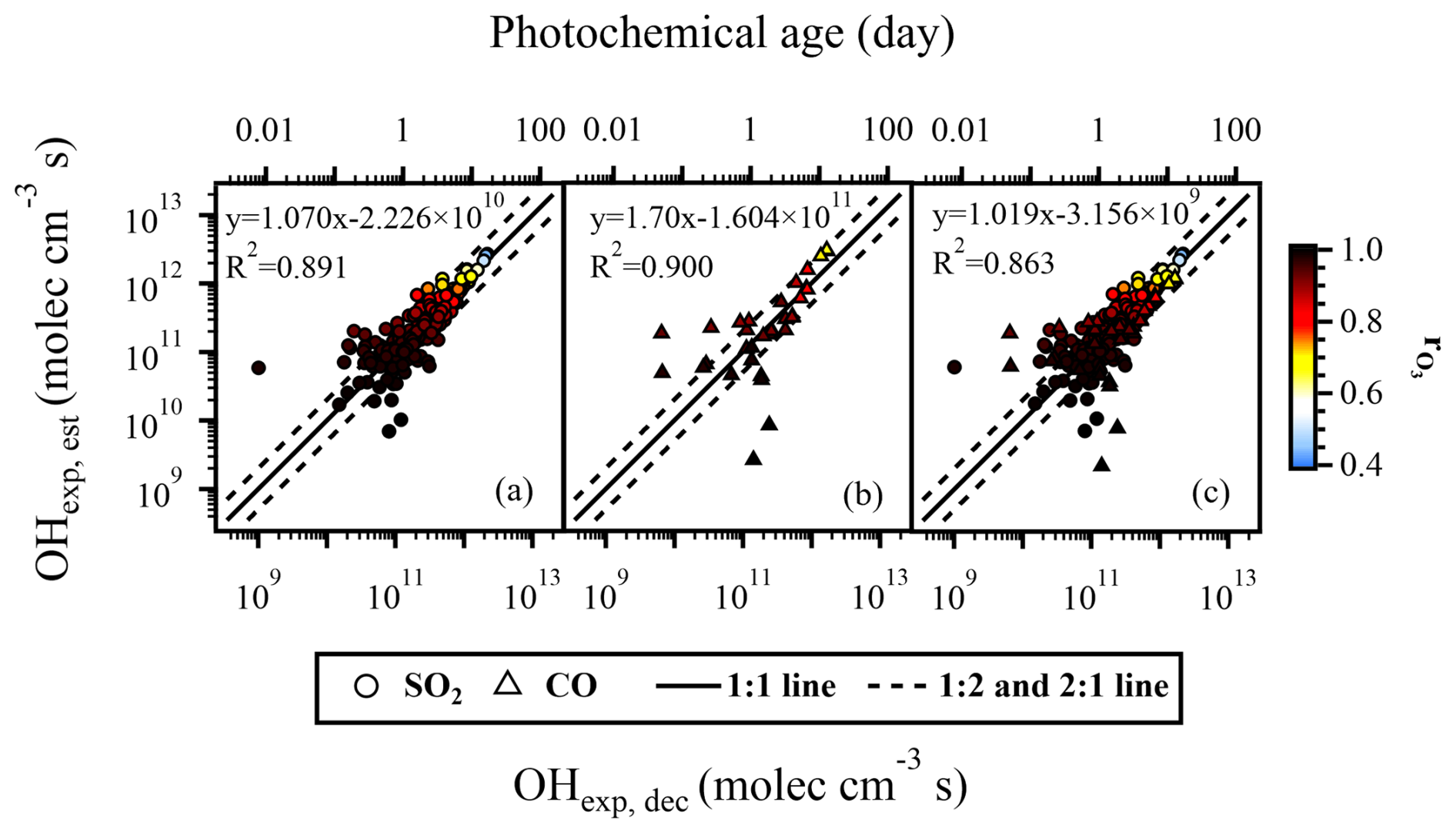
Figure 5 The regression results of OH_exp, dec and OH_exp, est in the OFR254 mode with (a) SO₂ and (b) CO as OHR_ext sources. (c) Results from all experiments (SO₂ and CO) in the OFR254 mode.

4 Conclusions

A series of OH_exp estimation experiments using the PAM-OFR were conducted in the OFR185 and OFR254 modes to explore the applicability of the empirical equations under a wide range of conditions. The results indicate that, for the OFR185 mode, when varying the residence time, water vapor mixing ratio, and output O₃ concentration (as a surrogate for UV intensity) within certain ranges, the empirical equation (Eq. 2) for OH_exp proves to be effective in estimating OH_exp. Unless there is a significant change in OHR_ext, such as transitioning from ambient conditions to emission source conditions, there is no need to refit the parameters a–f in the estimation equation to estimate OH_exp. Compared with the OFR254 mode, the consistency between OH_exp, est and OH_exp, dec in the OFR185 mode is better. For the OFR254 mode, when OHR_ext, input O₃ concentration, and $r_{{\mathrm{O}}_{\mathrm{3}}}$ vary within certain ranges, the empirical equation (Eq. 3) can be used to estimate OH_exp reasonably well using the parameters x–z obtained from a narrower range of data points. It is important to note that, for the OFR185 mode, the above conclusions are valid only if one already has a set of a–f values that are appropriate for the specific UV lamps being used, as the I₁₈₅:I₂₅₄ that affects the OH_exp is lamp-specific. For a PAM-OFR that employs a different Hg lamp, a series of calibration experiments should be conducted in any case. Alternatively, based on the research by Rowe et al. (2020), the exponential relationship between the a–f values and the I₁₈₅:I₂₅₄ could be used firstly to obtain a set of a–f values suitable for the UV lamps being used.

To obtain reliable estimates of OH_exp using Eqs. (2) and (3) for the OFR185 mode and the OFR254 mode, respectively, it is desirable to have sufficient data points (that is, OH_exp, dec from trace gas decay experiments) to fit the parameters for the calculation of OH_exp, est. There is currently no consensus on how many data points in trace gas decay experiments are enough for reliable fitted parameters, which could be important for in situ OH_exp estimation in field studies where a limited number of experiments are performed to reduce downtime. We aim to address this by random sampling from the data points in our experiments and determining the minimum number of experiments that are needed to obtain reliable OH_exp.

For the OFR185 mode, we firstly used randomly selected N data points from the 175 data points presented previously to fit the parameters (a–f) using Eq. (2). The fitted parameters were then used to reconstruct OH_exp, est for all 175 data points. The OH_exp, est values were then compared with the corresponding 175 OH_exp, dec values. This procedure was repeated 10 times for each N, with N starting from 7 and reaching approximately 50 (Fig. 6a). The average R², slope, and intercept from the 10 attempts were then shown as a function of N for experiments with SO₂ only (Fig. 6a) and for those with SO₂ and CO (Fig. 6b). It can be observed that around 30 data points are needed for experiments with SO₂ only, while around 20 data points are needed to have stable R² values and slopes when using both SO₂ and CO. For the OFR254 mode, the same procedure was applied to the 241 data points. It was not surprising that the results were a lot more scattered (Fig. 6c and d) compared to those for the OFR185 mode, given their performance shown in the previous section. Nevertheless, our analysis suggests that around 25 data points are needed to obtain reliable OH_exp, est for the OFR254 mode, whether using SO₂ alone (Fig. 6c) or SO₂ and CO (Fig. 6d) for the trace gas decay experiments. Therefore, despite the limitation that this practice only randomly samples the data points without considering the range of any experimental conditions, our analysis suggests that 20–30 data points are normally needed to obtain reliable OH_exp for both the OFR185 and OFR254 modes.

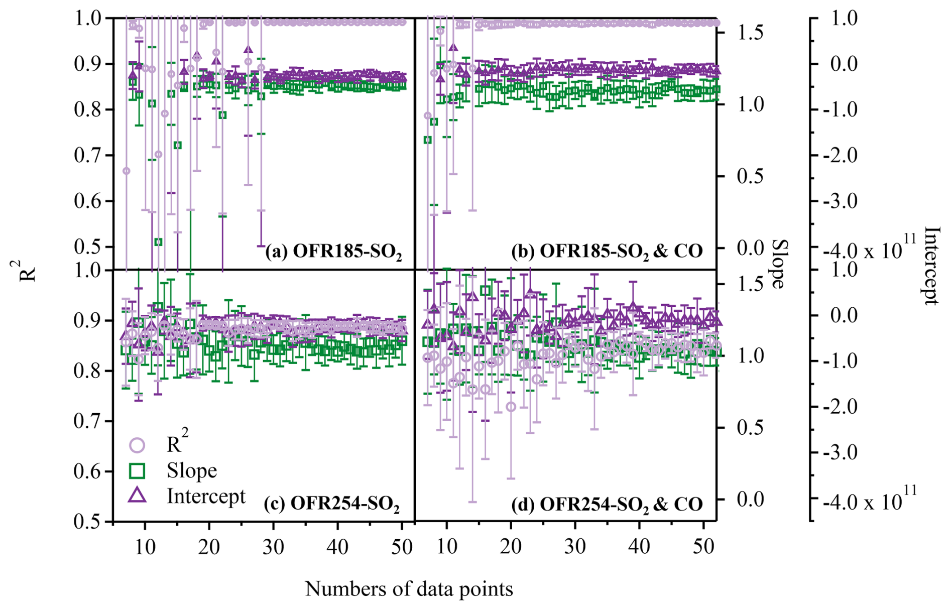
Figure 6 The regression results of OH_exp, dec and OH_exp, est (characterized by the R², slope, and intercept) when different numbers of data points were chosen. (a) SO₂ as the OHR_ext source in the OFR185 mode, (b) SO₂ or CO as the OHR_ext source in the OFR185 mode, (c) SO₂ as the OHR_ext source in the OFR254 mode, and (d) SO₂ or CO as the OHR_ext source in the OFR254 mode.

Our study suggests that the OH_exp, est estimated from the empirical equations agrees better with the OH_exp, dec for the OFR185 mode (Fig. 3) than for the OFR254 mode (Fig. 5). This can be understood from the perspective of OH generation and its consumption by OHR_ext (Li et al., 2015). For the OFR185 mode, there are two pathways to generate OH radicals: the photolysis of H₂O and the photolysis of O₃. For the OFR254 mode, the main pathway for OH radical generation is solely the photolysis of O₃. Consequently, when OHR_ext changes, the disruption to OH_exp in the system is more significant in the case of the OFR254 mode, while the OH_exp in the OFR185 mode remains more stable. In addition, pseudo-first-order kinetics between OH radicals and SO₂ or CO is assumed, with [OH] being at a pseudo-steady state. However, the relatively low OH radical generation capacity in the OFR254 mode might not necessarily always fulfill such an assumption, leading to higher uncertainties for estimating OH_exp. Therefore, the OFR185 mode offers certain advantages, such as relatively high OH_exp, more accurate OH_exp estimation, and no external input of O₃ needed. However, for substances that exhibit strong absorption at the wavelength of 185 nm and are prone to photolysis, such as aromatic species (Peng et al., 2016), using the OFR254 mode is a better choice. For users of other OFRs (non-PAM-OFR) who would like to apply the conclusions above, at least two conditions must be met: (1) the concentration of [OH] within the OFR should remain stable, and (2) the assumption of plug flow conditions should be acceptable, allowing the neglect of differences in the actual RTD, heterogeneity in the UV light intensity, and the concentration of radicals/oxidants at different points within the reactor, which are caused by different designs of reactors (such as wall materials, shapes, or volumes).