Assimilation of volcanic sulfur dioxide products from IASI and TROPOMI into the chemical transport model MOCAGE: case study of the 2021 La Soufrière Saint Vincent eruption with the March 2022 version of MOCAGE

Sulfur dioxide emitted during volcanic eruptions can be hazardous for aviation safety. As part of their activities, the Volcanic Ash Advisory Centres (VAACs) are therefore interested in the real-time atmospheric monitoring of this gas. A recent development aims at improving the forecasts of volcanic sulfur dioxide quantities made by the MOCAGE (Modèle de Chimie Atmosphérique à Grande Échelle) chemistry transport model. For this purpose, observations from both TROPOMI (Tropospheric Monitoring Instrument) and IASI (Infrared Atmospheric Sounding Interferometer; B and C) located on separate polar-orbiting satellites are assimilated into the model. These sulfur dioxide measurements are based on the eruption event of the La Soufrière Saint Vincent volcano in April 2021. Observations from OMI (Ozone Monitoring Instrument) are considered validation data. The resulting assimilation experiments show that the combined assimilation of IASI and TROPOMI observations always leads to a better forecast compared to the independent assimilation of data from each instrument. Sulfur dioxide atmospheric field forecasts are better when the available observations are numerous and cover a long time window.

1 Introduction

During volcanic eruptive events, large quantities of ash and sulfur dioxide (SO₂) are quickly released into the atmosphere. The emitted volcanic plumes can be transported far from the emission sources, sometimes reaching the upper troposphere or even the stratosphere (Carn et al., 2009). At such altitudes, volcanic ash plumes become hazardous for aviation safety as they can irreversibly damage aircraft engines and significantly lower flight visibility (Prata, 2009). Aircraft passengers and crew are also directly threatened, especially because air quality inside and at the vicinity of volcanic plumes is strongly degraded, generating respiratory issues detrimental to human health (Schmidt et al., 2014).

Volcanoes can be monitored by in situ sensors except if they are difficult to reach and hazardous. Consequently, passive satellite remote sensing remains an efficient technique providing global data on gases and aerosols emitted during volcanic eruptions. Sulfur dioxide is one of the compounds measurable by remote sensing. The absorbing bands of this gas are in the ultraviolet (UV; ∼ 310–340 nm) and thermal infrared (IR; − ν₁ ∼ 8.6 µm, ν₃ ∼ 7.3 µm and ν₁ + ν₃ ∼ 4 µm) domains (Carn et al., 2016).

In many eruption cases like the one of the Icelandic volcano Eyjafjallajökull in 2010, volcanic sulfur dioxide can be considered a tracer to predict volcanic ash dispersion (Sears et al., 2013). However, both ash and sulfur dioxide plumes need to be monitored separately as their spatial distribution do not always coincide perfectly (Thomas and Prata, 2011). A striking example is the case of the eruption of the Icelandic volcano Grímsvötn in 2011, during which both sulfur dioxide and ash plumes were clearly separated (Prata et al., 2017).

Volcanic sulfur dioxide primary emissions can also be rapidly converted into secondary sulfate aerosols by reacting with water vapour and dioxygen. This conversion directly impacts the spatial distribution of volcanic sulfur dioxide plumes. The eruption of the Hunga Tonga volcano in January 2022 was exceptional as volcanic gases (sulfur dioxide and water vapour) and ash have been injected at an altitude of at least 30 km (Witze, 2022). As a result, stratospheric sulfur dioxide has been rapidly converted into sulfate aerosols because of water vapour propelled into the stratosphere during the submarine eruption (Sellitto et al., 2022).

To guarantee aviation safety, pilots need to dispose of accurate data on volcanic plume extent, movement and chemical composition. The International Civil Aviation Organization (ICAO) and the World Meteorological Organization (WMO) created the International Airways Volcano Watch (IAVW) in 1987 for this purpose (Lechner et al., 2018). Since 1990, the IAVW system has included nine worldwide responsibility areas, each represented by a Volcanic Ash Advisory Centre (VAAC). Europe, Africa and the Middle East are part of the Toulouse VAAC supervised by Météo-France (Gouhier et al., 2020).

Information on volcanic plumes provided by each VAAC to aviation authorities currently relies on specific services like the Support to Aviation Control Service (SACS) (Brenot et al., 2014) or the European Natural Airborne Disaster Information and Coordination System for Aviation (EUNADICS-AV) (Brenot et al., 2021). Based on in situ measurements, satellite data and modelling products, these systems provide VAACs information on volcanic ash and sulfur dioxide plumes. The Toulouse VAAC forecasts the dispersion of volcanic ash plumes by running MOCAGE-Accident (Gouhier et al., 2020), a specific version of the three-dimensional chemistry transport model (CTM) MOCAGE (Modèle de Chimie Atmosphérique à Grande Échelle) of Météo-France. To achieve this, an injection profile and a quantity of ash emitted by the volcano, previously chosen by the forecaster, are used to predict the dispersion of the volcanic plume.

Assimilation of volcanic sulfur dioxide observations into a model has already been performed in several situations like for the eruption events of Eyjafjallajökull in 2010 and Grímsvötn in 2011. Volcanic sulfur dioxide released by these volcanoes has been monitored by the GOME-2 (Global Ozone Monitoring Experiment-2) and OMI (Ozone Monitoring Instrument) UV sensors. The resulting retrieved observations have been assimilated in the Integrated Forecasting System for atmospheric composition (IFS-COMPO) of the European Centre for Medium-Range Weather Forecasts (ECMWF) and improved the sulfur dioxide plume forecasts (Flemming and Inness, 2013). Volcanic sulfur dioxide retrievals from the GOME-2 and TROPOMI (Tropospheric Monitoring Instrument) UV sensor observations have been operationally assimilated in the global IFS-COMPO assimilation system since October 2020. On top of that, a retrieved volcanic sulfur dioxide layer height from the TROPOMI Layer Height product has been assimilated. Including plume height information into the assimilation system enhanced the quality of the forecasts made from the analysed fields (Inness et al., 2022).

The eruption of the La Soufrière Saint Vincent volcano emitted a large amount of SO₂ into the atmosphere between 9 and 22 April 2021. According to the study of Esse et al. (2024), around 380 kt of SO₂ was released into the atmosphere during the first 48 h of the eruption. This sulfur dioxide has been detected by several remote sensing instruments like the IR sensor IASI (Infrared Atmospheric Sounding Interferometer) and the UV sensors TROPOMI and OMI. The assimilation of TROPOMI, IASI and both instruments should improve MOCAGE. Indeed, without data assimilation, the model does not simulate the SO₂ plume. In this study, we jointly assimilate a UV instrument, TROPOMI, and the IR instruments IASI B and IASI C, allowing for the correction of the model during both day and night. The use of instruments with different wavelengths to assimilate volcanic SO₂ data is also beginning to be developed in IFS. In MOCAGE, a part of the SO₂ can be converted into sulfate aerosols, particles which are causing problems in the aviation sector.

For the assimilation, the three-dimensional variational data assimilation system of the CTM MOCAGE (El Amraoui et al., 2022) is used. Forecasts of volcanic sulfur dioxide plumes are then initialised by the resulting analyses. Two preliminary experiments are conducted by independently assimilating total columns retrievals from the IASI and TROPOMI sensors. The resulting total columns of volcanic sulfur dioxide assimilated in MOCAGE are then compared to those measured by the OMI independent sensor, located on another satellite.

In this paper, the La Soufrière Saint Vincent eruption event of 2021 is introduced in the second part. Then, the assimilation data provided by the corresponding instruments are described in the third part, before the chemical transport model MOCAGE and its assimilation system in the fourth part. The fifth part addresses the results of this case study.

2 Description of the 2021 La Soufrière Saint Vincent eruption

La Soufrière Saint Vincent is a volcano located in the Grenadine Islands (13.33° N, 61.18° W). The eruption in 2021 started on 9 April with a violent explosion around 12:40 UTC. This first explosion released a volcanic plume that reached an altitude of 8 km. As a result, thousands of people were forced to flee. A second and weaker explosion occurred at 18:45 UTC, generating a volcanic plume that reached an altitude of 4 km. At 22:35 UTC, a third explosion took place with a plume reaching 16 km. Between 10 and 11 April in the morning, the volcanic activity became periodic as explosions occurred every 1 to 3 h, during short time periods of 20 to 30 min each. Although the number of explosions decreased from 12 April, the volcanic plume remained at a high altitude, exceeding 12 km and sometimes even 16 km. Two last major explosions took place on 12 April at 08:15 UTC and on 13 April at 10:30 UTC with plumes reaching altitudes of 12.8 and 11 km respectively. The volcano continued to emit temporarily ash and volcanic gases in the atmosphere until 22 April, but the plume from these explosions no longer reached 8 km high. No fewer than 30 explosions were observed during this eruption event, most of them during 9 and 11 April. More information about the La Soufrière eruptions is available in the report of Bennis and Venzke (2021).

3 Description of the instruments

3.1 TROPOMI

TROPOMI is a hyperspectral radiometer with spectral bands extending from the UV to the shortwave infrared (SWIR) domains. This instrument is on board the polar-orbiting Sentinel 5 Precursor (S5p) satellite, whose goal is to provide information and services on air quality and climate (Reshi et al., 2024). Since August 2019, TROPOMI has benefited from a high spatial resolution of 5.5 km × 3.5 km at nadir. This instrument has a daily temporal resolution (no observation at night), and its local overpass time occurs at 13:35 UTC (Veefkind et al., 2012).

Volcanic sulfur dioxide plumes can be globally monitored with the high spatial resolution of TROPOMI. Unprocessed radiances measured by the instrument are often unpacked and formatted to become level 1 (L1) data. These data can then be converted into a proper retrieved environmental variable as sulfur dioxide, forming a level 2 (L2) product. This conversion requires the use of a retrieval algorithm having its own specificities and uncertainties. Historically, the first institutes studying sulfur dioxide L2 products with TROPOMI measurements were the Royal Belgian Institute for Space Aeronomy (BIRA) and the German Aerospace Center (Deutsches Zentrum für Luft- und Raumfahrt, DLR). For that, they use the differential optical absorption spectroscopy (DOAS) algorithm, particularly fitted for TROPOMI operational near-real-time processing (Reshi et al., 2024).

Backscattered ultraviolet radiation is measured in order to construct absorption spectra. The DOAS algorithm is then applied to these spectra for different fitting windows between 310 and 390 nm. The DOAS algorithm operates over several steps. First, slant column densities (SCDs) are computed. They correspond to the integrated sulfur dioxide concentration along the mean atmospheric optical path. Then, conversion factors called air mass factors (AMFs) are obtained from suitable radiative transfer calculations to take measurement sensitivity changes into account. These changes depend on many factors like observation geometry, total ozone absorption, clouds and surface reflectivity. Moreover, the measurement sensitivity varies with the altitude of the emitted sulfur dioxide plume. As this altitude is unknown, the AMFs are computed for several hypothetical sulfur dioxide vertical profiles. One profile used for polluted scenarios comes from a forecast made by the TM5 chemical transport model (Huijnen et al., 2010). Three other profiles are available for 1 km thick boxes. The first box extends from the ground level to 1 km high. The two others are centred at 7 and 15 km above mean sea level. The first profile is located in the boundary layer and stands for well-mixed anthropogenic or volcanic sulfur dioxide conditions. The second profile aims at representing sulfur dioxide emitted by effusive volcanic eruptions in the upper troposphere. The third one is for sulfur dioxide released by explosive volcanic eruptions above the lower stratosphere (Theys et al., 2017). As four AMFs are available depending on different assumed SO₂ vertical profiles, the conversion of SCDs into vertical column densities (VCDs) generates four types of VCDs. These vertical columns correspond to the number of sulfur dioxide molecules in an atmospheric column per unit area, usually expressed in Dobson units (1 DU = 2.69×10¹⁶ molec. cm⁻²). Finally, averaging kernels are computed for the four vertical profiles (Theys et al., 2019).

For our study, we use sulfur dioxide total vertical columns computed from the hypothetical profile centred around 15 km. These columns are associated with their systematic errors in order to compute the observation error matrix of the MOCAGE assimilation system. Moreover, the averaging kernel matrix needs to be considered for comparing TROPOMI to other instrumental measurements or model calculations (Rodgers and Connor, 2003). Finally, data are selected according to the category of the TROPOMI detection. Many cases are taken into consideration in our study: flag 1 for sulfur dioxide detection, flag 2 for clear volcanic detection and flag 3 for detection close to a known anthropogenic source. The quality of the SO₂ retrieval is given by a quality flag with values ranging from 0 for uncertain retrieval to 1 for the best retrieval. TROPOMI data are available on the NASA website (https://disc.gsfc.nasa.gov/, last access: 19 September 2024).

3.2 TROPOMI Layer Height product

The TROPOMI Layer Height product (Hedelt et al., 2019) allows for determining the altitude of an SO₂ plume when TROPOMI SO₂ total columns are higher than 20 DU thanks to a machine learning algorithm called the Full-Physics Inverse Learning Machine (FP_ILM). Hedelt et al. (2019) used the LInearized Discrete Ordinate Radiative Transfer (LIDORT) model (Spurr et al., 2008) to simulate many reflectance spectra for different values of the solar zenith angle (SZA), viewing zenith angle (VZA), relative azimuth angle (RAA), O₃ and SO₂ vertical column density, layer height, surface albedo, and surface pressure. Before separating these reflectance spectra into 10 principal components (PCs), the TROPOMI spectral response function, characterising the sensitivity of the instrument across its measurement spectrum, is applied. These PCs and information about the surface, O₃ total columns, SZA, VZA and RAA are used as input for the neural network. SO₂ total columns and SO₂ height are diagnosed thanks to the neural network. In this study, SO₂ total columns diagnosed by the neural network are not assimilated. Nevertheless, the SO₂ height product is used to validate the altitude of the modelled plume.

TROPOMI Layer Height data are available on the NASA website (https://disc.gsfc.nasa.gov/, last access: 12 April 2024). Older data were provided by the German Aerospace Center (DLR).

3.3 IASI

IASI is a Fourier transform spectrometer operating in the IR spectral domain. This instrument is located on both polar-orbiting MetOp-B (IASI B) and MetOp-C (IASI C) satellites. The best spatial resolution at nadir is a circle with a diameter of 12 km. Twice a day (measurements are possible both during daytime and nighttime), the IASI instruments observe at around 09:30 and around 21:30 local time (LT) (Clerbaux et al., 2009).

Sulfur dioxide observation data provided by IASI measurements are converted into a level 2 product using the ULB-LATMOS retrieval algorithm (Clarisse et al., 2012). In our study, we use an optimal sulfur dioxide total vertical column computed from an estimated altitude of the volcanic plume. This estimation is based on another algorithm created for IASI sulfur dioxide plume altitude retrievals (Clarisse et al., 2014). IASI data are available at the AERIS data centre (https://iasi.aeris-data.fr/, last access: 19 September 2024).

3.4 OMI

OMI is a multispectral radiometer with spectral bands extending from the UV to the visible (VIS) domains. This sensor is carried by the polar-orbiting Earth Observing System (EOS) Aura satellite. The best nadir spatial resolution is about 24 km × 13 km. Since 2011, this instrument has had 2 d daily coverage with an overpassing at 13:45 LT (Qu et al., 2019).

OMI sulfur dioxide total vertical columns are used as independent observations to check the results of our assimilation experiments. These total vertical columns are retrieved thanks to an algorithm based on a principal component analysis (PCA) technique (Li et al., 2017). These vertical columns are computed by considering a hypothetical sulfur dioxide plume altitude located around 18 km. OMI data are available on the NASA Earthdata website (https://omisips1.omisips.eosdis.nasa.gov/outgoing/OMSO2NRTb/, last access: 19 September 2024).

4 Description of the SO₂ assimilation experiments

MOCAGE (Modèle de Chimie Atmosphérique à Grande Échelle) is the CTM developed by the Centre National de Recherches Météorologiques (CNRM) at Météo-France (Josse et al., 2004). It has many operational uses such as air quality forecasting over France (Rouil et al., 2009) and over Europe, contributing data to the CAMS ensemble forecasting system (Marécal et al., 2015). MOCAGE is also used in a configuration without chemical reactions by the Volcanic Ash Advisory Centre of Toulouse (VAAC) when a volcanic eruption or an industrial accident occurs.

4.1 The model and its assimilation system

The CTM MOCAGE is a model using a semi-Lagrangian scheme for the transport of chemical species which can be global or nested. It enables predicting chemical evolution of the atmosphere up to 4 d. In this study, we use MOCAGE on a 1° global domain with 47 hybrid σ pressure levels distributed between the surface and 5 hPa (7 in the planetary boundary layer, 20 in the free troposphere and 20 in the stratosphere).

MOCAGE is an offline model and needs meteorological fields like wind speed and direction, temperature, humidity, pressure, rain, and clouds from a numerical weather prediction (NWP) model or from a climate model. In this study, meteorological forcings are provided by the French NWP model Action de Recherche Petite Echelle Grande Echelle (ARPEGE) (Courtier et al., 1991; Bouyssel et al., 2022).

The model enables transforming species according to the chemical scheme RACMOBUS, which is a combination of two chemical schemes. The first one, RACM, is computed for tropospheric chemical reactions (Stockwell et al., 1997). It is completed with the sulfur cycle (Feinberg et al., 2019). The second chemical scheme, REPROBUS, is used for stratospheric chemical reactions (Lefevre et al., 1994). Every 15 min, the MOCAGE model provides the atmospheric composition of 112 gaseous species thanks to 379 chemical reactions and 57 photolysis reactions.

Both primary and secondary aerosols are modelled in MOCAGE (Guth et al., 2016; Sič et al., 2015). Primary aerosols include desert dust, sea salt, black carbon, organic carbon and volcanic ash. In this study, volcanic ash modelling is turned off. Secondary inorganic aerosols are represented by sulfate, nitrate and ammonium aerosols. The aerosol size distribution is described by a sectional approach, with six size sections delimited by the following diameters: 0.002–0.01, 0.01–0.1, 0.1–1.1, 1.1–2.5, 2.5–10 and 10–50 µm. Desert dust and sea salt emissions depend on the wind strength and the type of the ground.

To forecast air quality, emissions of gaseous and aerosol species need to be taken into account by the model. Emission inventories are therefore used, such as the MACCity inventory for anthropogenic emissions (Lamarque et al., 2010) and the MEGAN inventory for biogenic emissions (Sindelarova et al., 2014). Sulfur dioxide released into the atmosphere by passive degassing can also be, as in our study, part of the emissions included in the model (Lamotte et al., 2021). Daily emissions of biomass burning provided by the Global Fire Assimilation System (GFAS) (Kaiser et al., 2012) are injected into the model at different vertical levels, depending on the latitude of fires (Cussac et al., 2020). Biomass burning emissions are injected at an altitude of 1 km in the tropics, 2 km at middle latitudes and 6 km at high latitudes. Other species except lightning nitrogen oxides (NO_x) (Price et al., 1997) and aircraft emissions (Lamarque et al., 2010) are emitted in the first five levels of the model (approximately 500 m altitude).

Many products can be assimilated in MOCAGE. For example, to improve O₃ in MOCAGE, total columns (Emili et al., 2014) or radiances (El Aabaribaoune et al., 2021; Vittorioso et al., 2024) can be assimilated. For the aerosols, aerosol optical depth (AOD) (Sič et al., 2016; El Amraoui et al., 2022) or lidar observations (El Amraoui et al., 2020; Cornut et al., 2023) can be assimilated into MOCAGE.

The assimilation system used in this study is 3D-VAR (three-dimensional variational assimilation), described hereafter. A short-range forecast from MOCAGE x^b and observations y are combined to find the optimal state x^a, taking into account their respective error covariance matrices B and R. x^a is the sum of x^b + δx^a, where δx^a is the increment minimising the cost function J:

$$\begin{array}{}\text{(1)}& \begin{array}{rl}J\left(\mathit{\delta }x\right)& ={\displaystyle \frac{\mathrm{1}}{\mathrm{2}}}\left(\mathit{\delta }x{)}^T{\mathbf{B}}^{-\mathrm{1}}\right(\mathit{\delta }x)+{\displaystyle \frac{\mathrm{1}}{\mathrm{2}}}{\left(y-\mathcal{H}\left[x^b\right]-\mathcal{H}\left[\mathit{\delta }x\right]\right)}^T\\ & {\mathbf{R}}^{-\mathrm{1}}\left(y-\mathcal{H}\left[x^b\right]-\mathcal{H}\left[\mathit{\delta }x\right]\right),\end{array}\end{array}$$

where ℋ is the observation operator used to obtain the model data in the observation space. Before running an assimilation experiment, a full description of the R and B matrices is required. The background error covariance is spread in space thanks to the correlation matrix described in El Amraoui et al. (2020). This matrix contains both horizontal and vertical components.

The horizontal correlation $C_{m,n}^{\mathrm{h}}$ between two points m and n is defined as follows:

$$\begin{array}{}\text{(2)}& C_{m,n}^{\mathrm{h}}=\exp \left[{\displaystyle \frac{-d^{\mathrm{2}}}{\mathrm{2}\left(L_{x^{\mathrm{2}}}+L_{y^{\mathrm{2}}}\right)}}\right],\end{array}$$

where d is the distance between the points m and n and L_x and L_y are the longitude and latitude length scales in kilometres. In our study, the longitude and latitude length scales are equal to one mesh grid (1°).

In kilometres, the length scales become

$$\begin{array}{}\text{(3)}& L_x=L_y=\mathrm{2}{R}_{\mathrm{e}}\cdot \sin \left({\displaystyle \frac{\mathit{\pi }}{\mathrm{360}}}\right),\end{array}$$

where R_e is Earth's radius (6371.22 km).

The vertical correlation $C_{i,j}^{\mathrm{v}}$ between two pressure levels (p_i and p_j) is defined as follows:

$$\begin{array}{}\text{(4)}& C_{i,j}^{\mathrm{v}}=\exp \left[-\mathrm{100}\cdot {\left[\log \left({\displaystyle \frac{p_i}{p_j}}\right)\right]}^{\mathrm{2}}\right].\end{array}$$

In our study, the values of the vertical correlation between two consecutive levels are set to 1.

4.2 TROPOMI and IASI data assimilation setup

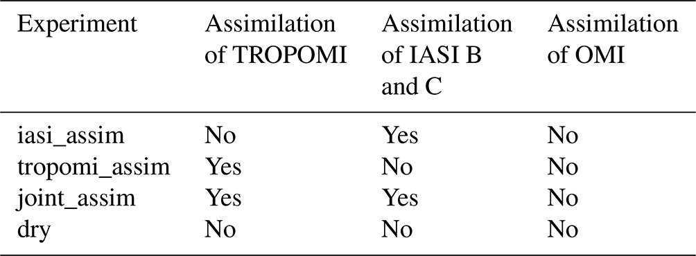
Several hourly 3D-VAR assimilations of volcanic SO₂ data into MOCAGE have been conducted over the specific eruptive period from 9 to 15 April 2021 with a 1° horizontal resolution. Different simulations have been carried out: one with the assimilation of IASI B and C (iasi_assim), one with the assimilation of TROPOMI (tropomi_assim), another with the assimilation of IASI and TROPOMI, and the last one without assimilation (Table 1). The results of these experiments are compared to OMI observations.

Table 1 Description of the experiments performed during this study with the different assimilated instruments.

In these experiments, IASI and OMI observations above 0.5 DU are used. This value corresponds to the lowest total columns measurable by these instruments (Koukouli et al., 2022; Qu et al., 2019). For TROPOMI, observation retrievals with an SO₂ peak concentration at 15 km altitude are used. Moreover, an observation is used when the quality flag is above 0.5 and if the slant column is above 1 DU, matching the noise of the instrument.

Averaging kernels are taken into account in this study. For TROPOMI, averaging kernels are only given for the a priori profiles from the TM5 CTM. Nevertheless, averaging kernels for the other a priori profiles can be estimated by multiplying them by a scaling factor (Theys, 2018) as described by the following equation:

$$\begin{array}{}\text{(5)}& \text{AVK}\left(z\right)={\displaystyle \frac{{\text{AVK}}_{\mathrm{TM}\mathrm{5}}\left(z\right)\times {\text{AMF}}_{\mathrm{TM}\mathrm{5}}\left(z\right)}{{\text{AMF}}_{\mathrm{15}\mathrm{km}}}},\end{array}$$

where AVK(z) is the averaging kernels at a given altitude, AVK_TM5(z) and AMF_TM5(z) are the averaging kernels and the air mass factor at altitude z from the TM5 CTM, and AMF_15 km is the air mass factor for the a priori profile containing a peak at 15 km altitude.

For IASI, averaging kernels are not given in the observation files. However, they can be computed at many heights thanks to the SO₂ total columns, according to the following equation:

$$\begin{array}{}\text{(6)}& \text{AVK}\left(z\right)={\displaystyle \frac{Y\left(z\right)}{Y\left(z_{\mathrm{ref}}\right)}},\end{array}$$

where z is the hypothetical SO₂ injection altitude, AVK(z) is the averaging kernels at a given altitude z, Y(z) is the total columns computed for an SO₂ injection at altitude z and Y(z_ref) is the total column computed for a reference altitude injection. In our case, this altitude is provided by the observation files.

In this study, we assume there is no spatial correlation in the observation error. For TROPOMI, the observation error standard deviation (sigR) is set according to the uncertainties provided by the instrument for each observation (Fig. 1a). The observation error standard deviation is set to around 25 % of the observations for TROPOMI. The uncertainties in IASI measurements vary according to the value of the total column measured. In the case of this eruption, IASI measured total SO₂ columns ranging from 0.5 to 20 DU. The uncertainties in this range of observations vary from around 25 % to 5 % of the observation (Clarisse et al., 2012). For IASI, we set the observation error standard deviation to 15 % of the observation values (Fig. 1b).

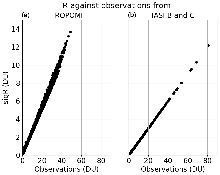
Figure 1 Values of the observation error standard deviation (sigR) according to TROPOMI (a) and IASI (b) observations.

For observations greater than 20 DU, the TROPOMI Layer Height product is able to diagnosed the altitude of the plume. During this volcanic eruption, 90 % of the diagnosed heights are between 9 and 21 km. Consequently, to force SO₂ injection between these two altitudes, we chose a profile containing strong values ($\mathrm{1}\times {\mathrm{10}}^{-\mathrm{8}}$ ppv) between altitudes of 9 and 21 km as the background error standard deviation. It is important to note that this setting of the background error standard deviation is only valid for this volcanic eruption and that, for another eruption, the user must choose a different profile of the background error standard deviation to inject SO₂ at the correct altitude into the model. The correlation matrix is the same in all experiments with data assimilation.

As in the operational mode of MOCAGE, a forecast initialised by the assimilation outputs is launched at 00:00 UTC each day. In our study, this forecast is performed for up to a 72 h term range.

5 Impact on analyses

5.1 Impact on SO₂ and sulfate

Figure 2 shows the SO₂ total columns observed and analysed on 10 April 2021 at various times (02:00, 14:00, 16:00 and 17:00 UTC). The observations are depicted on the first line for TROPOMI and the second and the third lines for IASI B and C respectively. The model's outputs are on the fourth line for the iasi_assim experiment, on the fifth line for the tropomi_assim experiment and on the sixth line for the joint_assim experiment. At 02:00 UTC, the tropomi_assim simulation does not present an SO₂ plume, in contrast to the plume modelled with IASI assimilation. Nevertheless, the model underestimates the total column values as compared to the IASI observations. Due to the use of UV wavelengths, TROPOMI is unable to measure SO₂ total columns at night. Consequently, no SO₂ plume is modelled in MOCAGE until 17:00 UTC. Before the overpass of TROPOMI, IASI instruments measure SO₂ total columns once again. It allows for increasing both the intensity and size of the plume in MOCAGE at 14:00 UTC. At 17:00 UTC, a plume appears in the tropomi_assim experiment thanks to the TROPOMI overpass. Compared to the TROPOMI observations, values of high total columns are underestimated by MOCAGE. At this time, the simulated volcanic plume in the iasi_assim experiment is slightly smaller and weaker than the plume in the tropomi_assim experiment and the TROPOMI observations. Assimilation of TROPOMI data allows for simulating a strong area value in the vicinity of the volcano in both the tropomi_assim and joint_assim experiments. This structure of strong values is not modelled with the IASI data assimilation because it corresponds to the latest volcanic SO₂ emission. This new release, due to a new eruption event, took place between the IASI and the TROPOMI overpasses. Simulated SO₂ total columns in the joint_assim experiment are stronger, in particular around 55° W, where observations are strong. For this part of the plume, the difference between the model and the observations is weaker because it is analysed five times during this day, whereas the model is corrected four times when IASI is assimilated and only once when TROPOMI is assimilated. The greater the number of model corrections, the smaller the differences between observations and the model. In this experiment, the shape of the plume is slightly different with a pattern around 39° W, which is simulated with the IASI data assimilation and not with the TROPOMI one.

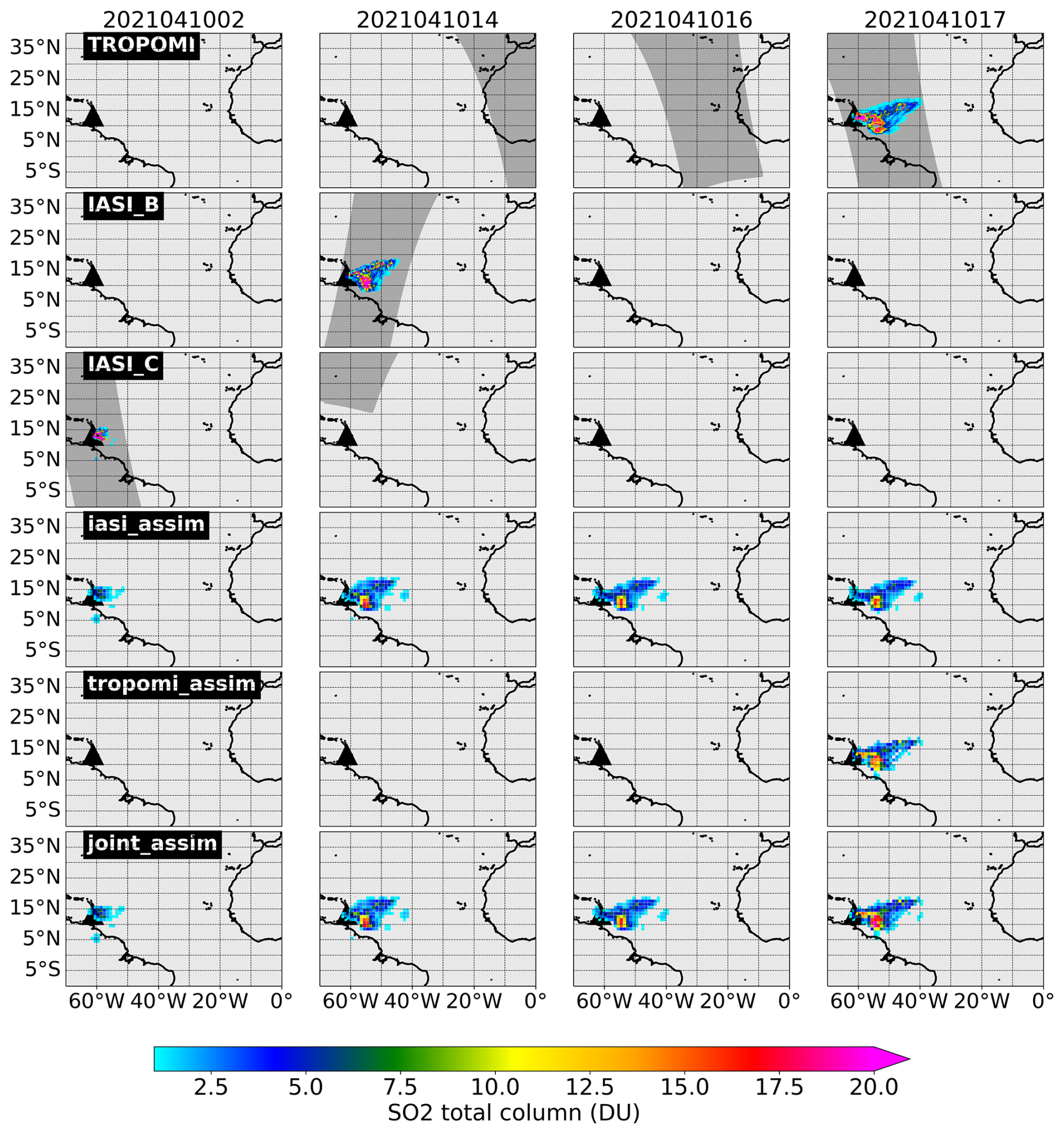
Figure 2 Observations assimilated and analyses of SO₂ total columns on 10 April 2021 at 02:00, 14:00, 16:00 and 17:00 UTC. The first three rows correspond to TROPOMI, IASI B and IASI C observations respectively. Analysis outputs are plotted on the fourth line for the iasi_assim experiment, on the fifth line for the tropomi_assim experiment and on the sixth line for the joint_assim experiment. The shaded areas on the first three lines correspond to areas where there are no observations or where observations have not been assimilated. Observations are not assimilated when they are less than 0.5 DU for IASI and TROPOMI's slant columns are less than 1 DU.

Figure 3 shows the SO₂ total columns observed and analysed on 11 April 2021 at 11:00, 13:00, 17:00 and 18:00 UTC. Until but not including 17:00 UTC, the SO₂ plumes simulated by the iasi_assim and the joint_assim experiments are similar. At 11:00 UTC, the eastern parts of the plume are consistent between experiments. Thanks to the IASI overpass at the end of the previous day, the plume is closer to the volcano and SO₂ total columns of the western part of the plume are stronger compared to the tropomi_assim experiment. At 13:00 UTC, IASI SO₂ total columns are assimilated, reducing the SO₂ plume over the ocean and increasing the values in the vicinity of the volcano in the model. At 17:00 UTC, TROPOMI observations are assimilated and the shape of the SO₂ plume is consistent between the experiments. The SO₂ plume is more extended with the assimilation of TROPOMI. Concerning the values of the total columns, areas with high values are more intense regarding the assimilation of both instruments, particularly near the volcano and in the middle of the Atlantic Ocean. At 18:00 UTC, the OMI overpass enables validating these experiments with independent observations. The SO₂ plume simulated by the joint_assim experiments seems to be the closest to OMI observations. Indeed, in this experiment, the strong SO₂ total column patterns match better to the observations, in particular around 39 and around 55° W.

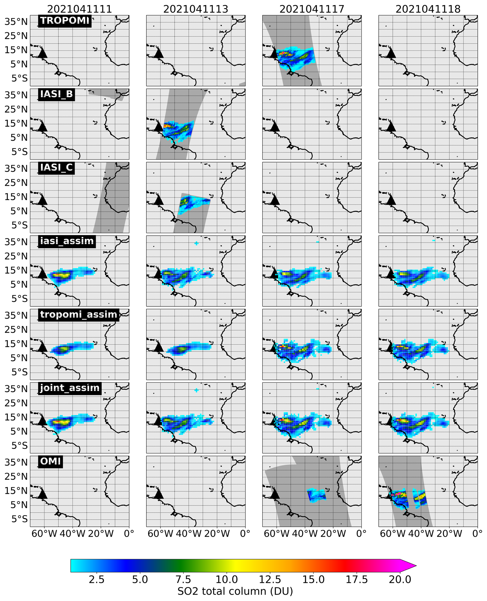
Figure 3 Observations and analyses of SO₂ total columns on 11 April 2021 at 11:00, 13:00, 17:00 and 18:00 UTC. The first three rows correspond to TROPOMI, IASI B and IASI C observations respectively. The last row corresponds to OMI observations. Analysis outputs are plotted on the fourth line for the iasi_assim experiment, on the fifth line for the tropomi_assim experiment and on the sixth line for the joint_assim experiment.

The vertical cross-section at 13.5° N, illustrated in Fig. 4, presents the vertical SO₂ concentrations at various times on 11 April 2021 (11:00, 13:00, 17:00 and 18:00 UTC). The chosen assimilation settings result in a plume that extends from 9 to 21 km in altitude. Until but not including 17:00 UTC, the altitude of the maximum SO₂ concentration in the different experiments is consistent with an altitude around 13 to 17 km. The lowest concentrations are simulated in the tropomi_assim experiment. At 11:00 UTC, the IASI assimilation of the end of the previous day enables simulating a plume located closer to the volcano compared to the tropomi_assim experiment. At 13:00 UTC, with the assimilation of IASI, a new strong concentration pattern appears near the volcano around 13 km altitude. At 17:00 UTC, in experiments where TROPOMI observations are assimilated, SO₂ concentration increases around 9 km altitude in the vicinity of the volcano. The altitude of the plume is closer to the TROPOMI Layer Height product in the joint_assim experiment. However, around 50° W, the TROPOMI Layer Height product shows a plume between 10 and 16 km altitude. In the experiments, the height of the plume varies between 15 and 20 km, which is too high compared to the TROPOMI Layer Height product. Nevertheless, around 50° W, few observations meet the criteria for the TROPOMI Layer Height product to be able to diagnose the height of the plume. It is difficult to conclude whether the plume altitude is correctly represented in the model when there are few or no observation above 20 DU.

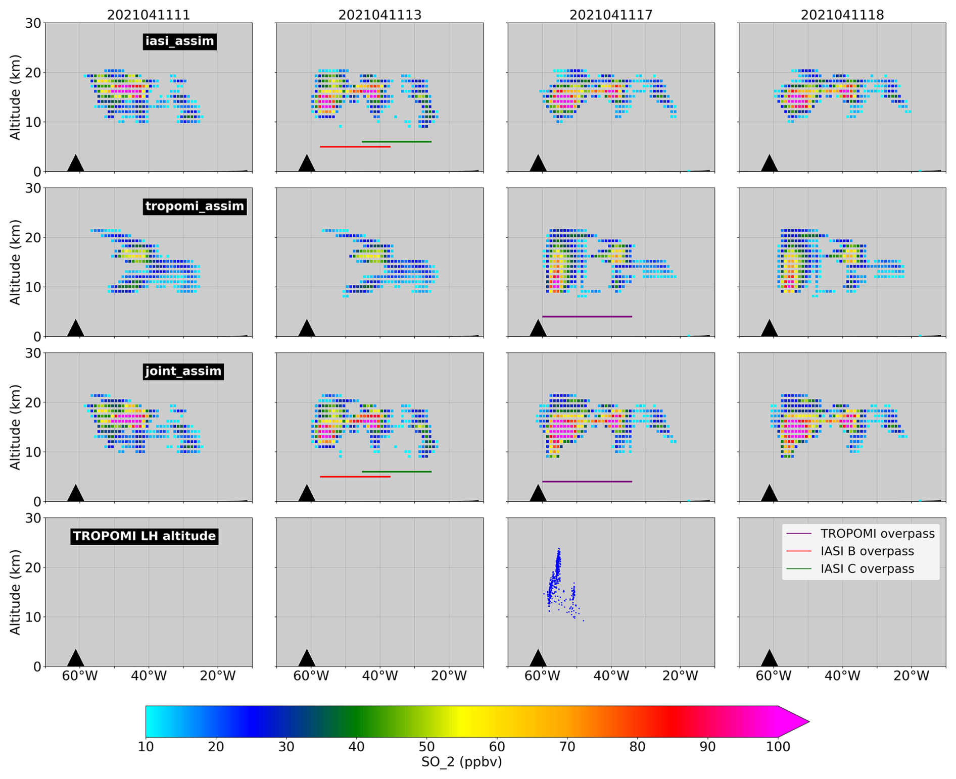
Figure 4 Vertical sections of the analysed SO₂ concentration at 13.5° N on 11 April 2021 at 11:00, 13:00, 17:00 and 18:00 UTC. Rows correspond to the TROPOMI data assimilation, IASI assimilation, joint assimilation and height of the SO₂ plume provided by the TROPOMI Layer Height product respectively.

SO₂ can be converted into sulfate aerosol in the presence of water vapour. This process is modelled in MOCAGE. Indeed, sulfate total columns show structures in the assimilation experiment which are not shown without assimilation.

Figure 5 shows the SO₂ total columns in the top panel, the sulfate total columns in the middle panel and the aerosol optical depth (AOD) in the bottom panel on 14 April 2021 at 07:00 UTC for different experiments with assimilation (iasi_assim, tropomi_assim and joint_assim) and without assimilation (dry). This figure shows strong differences between each experiment. Indeed, on this date, the analysed SO₂ total columns are stronger by assimilating TROPOMI than in the iasi_assim and the joint_assim experiments. Nevertheless, SO₂ total column values never reach 3 DU. Without assimilation, no SO₂ plume is modelled by MOCAGE.

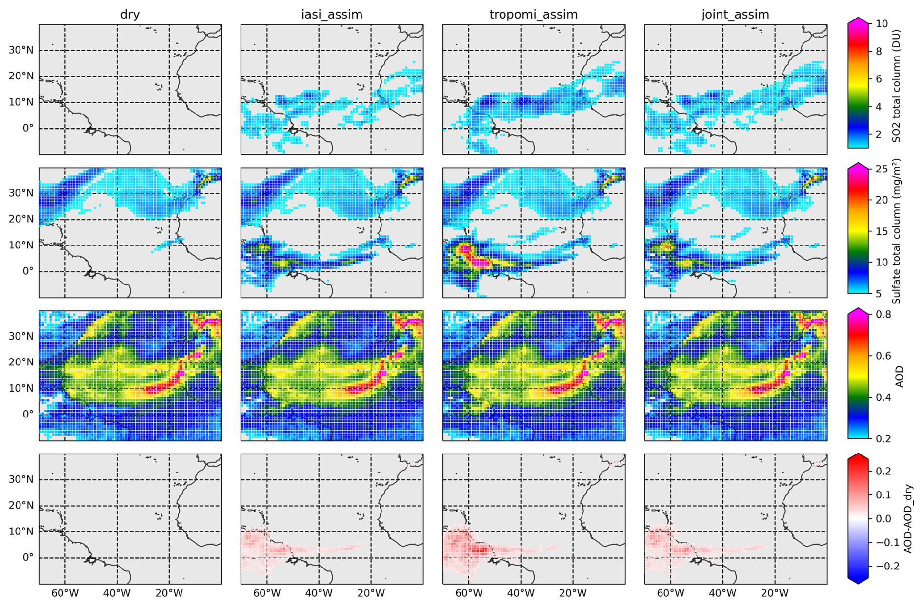
Figure 5 SO₂ total column, sulfate total column, AOD, and the difference between AOD and the AOD of the dry experiment on 14 April 2021 at 7:00 UTC for the dry, iasi_assim, tropomi_assim and joint_assim experiments.

The assimilation of volcanic SO₂ total columns allows the model to simulate sulfate aerosols (middle panel of Fig. 5). Indeed, a sulfate plume is simulated from the volcano to Guinea. This sulfate plume is not modelled in the experiment without assimilation. In the tropomi_assim experiment, strong sulfate total columns are simulated in French Guiana and in Venezuela. In this area, values exceed 25 mg m⁻², whereas values do not reach 20 mg m⁻² in the iasi_assim and joint_assim experiments. Elsewhere the modelled sulfate total columns are consistent with from one assimilation experiment to another.

Total AOD values slightly increased in Central America with the SO₂ assimilation (fifth line in Fig. 5). This rise is more important regarding assimilating TROPOMI in French Guiana and in Venezuela, where AOD values reach 0.5 compared to 0.4 in the iasi_assim and in the joint_assim experiments and 0.3 without assimilation (fourth line in Fig. 5). However, few AOD observations from the MODIS (Moderate-Resolution Imaging Spectroradiometer) and VIIRS (Visible Infrared Imaging Radiometer Suite) instruments are available in this area. This makes it impossible to validate AOD assimilation.

The assimilation of SO₂ total column measurements significantly enhances MOCAGE's ability to describe SO₂ plumes. When no observations are assimilated, no SO₂ plume is represented by the model. However, when satellite observations are assimilated, an SO₂ plume is simulated and corrected more or less frequently depending on the instrument or combination of instruments and thus on the overpass time of the corresponding satellites.

5.2 Impact of the assimilation on the detection of SO₂ threshold exceedances

To assess the impact of assimilation on volcanic SO₂, the number of grid cells reaching the 1 and 5 DU thresholds, over a sub-domain extending from 90° W to 40° E and from 20° S to 30° N, has been calculated and plotted in Fig. 6 for the iasi_assim (in red), tropomi_assim (in blue) and joint_assim (in green) simulations and for the TROPOMI (in orange), IASI B (in purple), IASI C (in magenta) and OMI (in grey) observations. Since there are often several observations per grid cell, we looked at the number of grid cells where the minimum and maximum of the total columns exceed these thresholds. These values are represented by horizontal lines. The number of grid cells where the median of the observations is higher than these thresholds is shown by a dot. Finally, the limits of the bars represent the number of grid cells where the 25th and 75th quantiles exceed the thresholds.

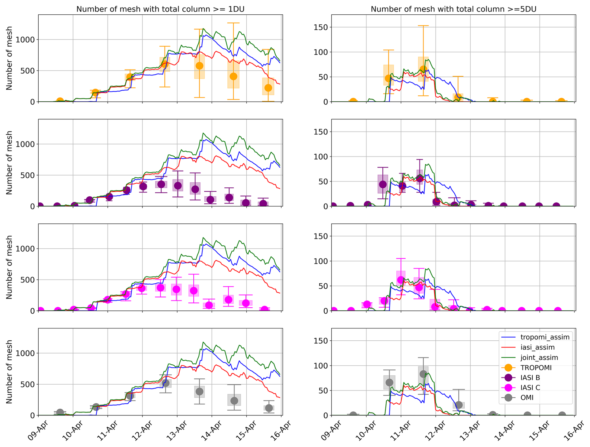
Figure 6 Number of grid cells where analyses exceed 1 and 5 DU. The blue, red and green lines show the number of points at which the total columns reach these thresholds in the tropomi_assim, iasi_assim and joint_assim experiments. Orange, purple, magenta and grey boxplots represent the number of grid cells where TROPOMI, IASI B, IASI C and OMI observations exceed the threshold.

Between 9 and 11 April 2021, the number of meshes where the median of the observations exceeded 1 DU is consistent between instruments. After this date, there were more grid cells where the median number of observations exceeded 1 DU with TROPOMI. Moreover, with this instrument, the dispersion of observations is high. There are few grid cells where all the observations exceed 1 DU, whereas on 14 April, there were more than 1200 grid cells where the maximum number of observations reaches 1 DU. This dispersion is lower for instruments with lower resolutions. For IASI, the number of grid cells where the median of observations is greater than or equal to 1 DU varies less than with UV instruments. This can be explained by IASI's high sensitivity to water vapour, which masks part of the SO₂ column.

In the assimilation experiments, the number of points where the total column reaches 1 DU is identical between iasi_assim and joint_assim until the end of the day on 10 April 2021. Until this date, the number of grid cells where the total column reaches 1 DU is zero with the TROPOMI assimilation. After this date, the number of grid cells where the total column exceeds 1 DU is always bigger in the joint_assim experiment. The number of grid cells above 1 DU is lower when only TROPOMI is assimilated in the morning until 11 April. This number is smaller when only IASI is assimilated. The differences in the number of grid cells exceeding 1 DU are greater at the end of the study period. Until 11 April 2021 in the experiments where TROPOMI was assimilated and until 12 April 2021 with the assimilation of IASI alone, the number of grid cells where the model exceeded 1 DU was consistent with the number of grid cells where the median of the observations exceeded this threshold. After this date, the number of grid cells exceeding 1 DU exceeds the number of meshes where the 75th quantile of TROPOMI observations exceeds 1 DU. Whatever the instruments used, the number of points above 1 DU is too high compared to IASI and OMI observations. This shows that the extension of the SO₂ plume is too large in the model.

The number of grid cells with observations exceeding 5 DU is lower and similar for each instrument. On 9, 14 and 15 April 2021, none of the observations exceeded this threshold. In the model, no column exceeds 5 DU for these dates. Generally, the number of SO₂ columns exceeding 5 DU in the model is similar to the number of grid cells where the median of observations exceeds 5 DU. Between the end of the day on 10 and 12 April, the number of meshes in MOCAGE is slightly greater by assimilating the two instruments. Generally, this number is closer to the number of meshes where the median of the OMI observations reaches 5 DU except at the end of the day on 10 April 2021, when the number of meshes above 5 DU is slightly underestimated. On this day, this number is underestimated in the model because a new eruption took place between the last assimilation of TROPOMI and the overpass of OMI. On 11 April, the TROPOMI assimilation added a significant number of points above 5 DU in the model because of a large number of TROPOMI observations above 5 DU. On 12 April, the extension of the plume reaching 5 DU is greater when assimilated in the tropomi_assim experiment. In fact, the value of the total columns falls in the model thanks to the assimilation of IASI. The TROPOMI overpass at the end of the afternoon also reduces the modelled total columns. The number of points above 5 DU in the model becomes similar.

To assess the accuracy of the model in simulating SO₂ total columns, a threshold-based analysis was implemented. The goal was to determine the number of instances where both the observations and the model successfully identified SO₂ total columns above certain thresholds (labelled as hits), instances where the observations exceeded these thresholds but the model failed to detect them (labelled as misses), instances where the model exceeds these thresholds but the observations do not reach these thresholds (labelled false alarms), and instances where both the observations and the model successfully identified SO₂ total columns under certain thresholds (labelled as correct rejections). Using these numbers, we defined three metrics.

The first one is the probability of detection (POD), a ratio that ranges from 0 to 1. The POD is calculated by dividing the number of hits by the sum of hits and misses for a given threshold. A POD score of 1 indicates a perfect detection by the model, meaning that all observed instances above the threshold were correctly simulated. On the other hand, a POD of 0 signifies that none of the observed SO₂ total columns above the threshold were detected by the model. The POD is computed with the following equation:

$$\begin{array}{}\text{(7)}& \text{POD}={\displaystyle \frac{\text{hits}}{\text{hits}+\text{misses}}}.\end{array}$$

The second one is the critical success index (CSI), a ratio that ranges from 0 to 1. The CSI is calculated by dividing the number of hits by the sum of hits, misses and false alarms for a given threshold. A CSI score of 1 indicates perfect detection by the model, meaning that all observed instances above the threshold were correctly simulated. On the other hand, a POD of 0 signifies that none of the observed SO₂ total columns above the threshold were detected by the model. The CSI is computed with the following equation:

$$\begin{array}{}\text{(8)}& \text{CSI}={\displaystyle \frac{\text{hits}}{\text{hits}+\text{misses}+\text{false alarms}}}.\end{array}$$

The last one is the false alarm rate (FAR), a ratio that ranges from 0 to 1. The FAR is calculated by dividing the number of false alarms by the sum of false alarms and correct rejections for a given threshold. A FAR score of 0 indicates that there are only correct rejection instances. On the contrary, a FAR score of 1 indicates that there are only false alarm instances. The FAR is calculated with the following equation:

$$\begin{array}{}\text{(9)}& \text{FAR}={\displaystyle \frac{\text{correct rejections}}{\text{correct rejections}+\text{false alarms}}}.\end{array}$$

To study these metrics, the notations in Table 2 are adopted. For POD metrics, times when there are neither hits nor misses are shown by a dot and times when there are no hits but there are misses are represented by a cross. For CSI metrics, times when there are no hits, no misses and no false alarm are shown by a dot and times when there are no hits and no false alarms but misses occur are represented by a cross. If there are no hits but if there are misses and false alarms, a star is plotted. For FAR metrics, a dot is plotted when there are no false alarms and no correct rejections. A cross is plotted when there are no false alarms but there are correct rejections.

Table 2 Symbols used in the plots according to the studied metric and the number of hits, misses, false alarms and correct rejections.

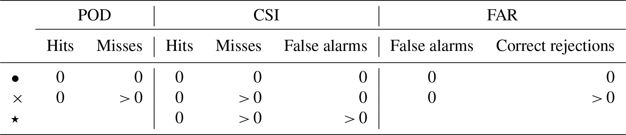
Figure 7 shows the probability of detection computed for the 1 and 5 DU thresholds against TROPOMI and IASI observations. Dots represent times when there is no observation. Crosses represent the moments when simulated SO₂ total columns are under a threshold, whereas some observations exceeds this threshold. Compared to TROPOMI, POD values are generally better in the experiments in which TROPOMI observations have been assimilated. In these experiments, POD values exceed 0.75. The POD values are over 0.75 until 12 April in the iasi_assim experiment except on 9 April. POD values decrease at the end of the study period. For the 5 DU threshold, POD values are slightly higher in the joint_assim experiment, especially on 10 and 11 April, when around 100 TROPOMI observations exceed 5 DU. On 12 April, POD values are around 0.4 in the experiments in which TROPOMI is assimilated. No SO₂ total column higher than 5 DU is simulated for this date in the iasi_assim experiment. Between 13 and 15 April and on 9 April, no SO₂ total column above 5 DU is simulated in MOCAGE. For these days, between one and nine observations above 5 DU are measured by TROPOMI.

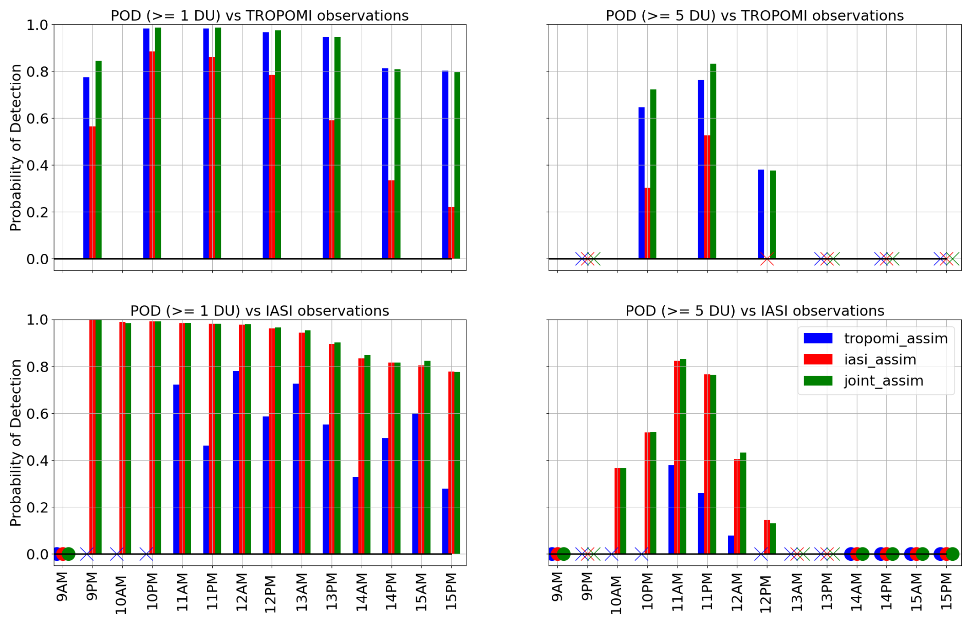
Figure 7 Probability of detection for the 1 and 5 DU thresholds for the three experiments: tropomi_assim in blue, iasi_assim in red and joint_assim in green. Dots represent times when there are no observations. Crosses represent the moments when there are only misses. AM: morning, PM: afternoon.

POD values, computed for a 1 DU threshold and with IASI observations, exceed 0.75 in experiments in which IASI instruments are assimilated. No SO₂ total columns are simulated with the TROPOMI assimilation until 10 April because TROPOMI overpasses the plume after IASI. On the morning of 9 April, no observation above 1 DU is detected by IASI. From 11 April, POD values vary between 0.3 and 0.8 in the tropomi_assim experiment. In this experiment, POD values are often higher in the morning. In the afternoon of 9 April, only one observation above 5 DU is measured by IASI. At this location, the total column is under 5 DU. For this threshold and compared to the tropomi_assim experiment, the probability of simulating high increases in SO₂ total columns thanks to the IASI assimilation. Despite numerous observations above 5 DU, many events are missed on 10 April with a POD reaching nearly 0.4 in the morning and 0.5 in the afternoon. Most of the simulated SO₂ total columns are between 1 and 5 DU. The maximum POD is obtained on 11 April after the assimilation of many observations measured by IASI exceeding 5 DU on 10 and 11 April.

The first line in Fig. 8 shows the POD computed against OMI observations for the 1 and 5 DU thresholds. On this line, dots represent times when there are no hits and no misses. Crosses represent the moments when simulated SO₂ total columns are under a threshold, whereas some observations exceed this threshold. The POD values computed with a 1 DU threshold are often consistent between the tropomi_assim and the joint_assim experiments. POD values are slightly better in the joint_assim experiment between 9 and 13 April. For the 5 DU threshold, POD value is greater with the joint_assim experiment on 10 and on 11 April. On 12 and 13 April, no SO₂ total column above 5 DU is modelled by MOCAGE, whereas OMI measured observations above this threshold. Elsewhere in the study period, no observation greater than 5 DU is measured by OMI and modelled by MOCAGE.

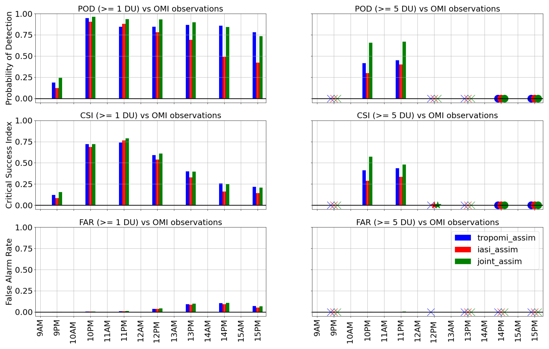
Figure 8 Probability of detection (first line), critical success index (second line) and false alarm rate (last line) for the 1 and 5 DU thresholds for the three experiments: tropomi_assim in blue, iasi_assim in red and joint_assim in green. The meaning of the symbols is described in Table 2.

The second line in Fig. 8 shows the CSI computed against OMI observations for the 1 and 5 DU thresholds. As for the POD, the CSI values computed with a 1 DU threshold are often consistent between the tropomi_assim and the joint_assim experiments. CSI values are slightly better in the joint_assim experiment on 9, 11 and 12 April. On 10 and 11 April, CSI values are around 0.75, whereas POD values are around 0.9. It means that there are few false alarms during this both days. On the contrary, from 13 April, CSI values are much lower than POD values. It means that the plume in MOCAGE becomes too large, leading to a lot of false alarms. For the 5 DU threshold, CSI values are better in the joint_assim experiment on 10 April and to a lesser extent on 11 April. From 14 April, no observations higher than 5 DU are measured by OMI and modelled by MOCAGE. On 9 and 12 April with the tropomi_assim experiment and on 13 April, there are no OMI observations greater than 5 DU but some values above 5 DU are simulated by MOCAGE. On 12 April, there are misses and false alarms in the iasi_assim and joint_assim experiments.

The third line in Fig. 8 shows the FAR computed against OMI observations for the 1 and 5 DU thresholds. The FAR values computed with a 1 DU threshold are similar between experiments. Up to 11 April, FAR values are approximatively equal to 0. This shows that the number of correct rejections is larger than the number of false alarms. The FAR values increases from 12 April, meaning that the plume is too large in the model. The FAR values computed with the 5 DU threshold are always close to 0. On 9 and 12 April in the tropomi_assim experiment and from 13 April, there are only correct rejections.

In the various modelling experiments, assimilating SO₂ total column data enhances the performances of the CTM MOCAGE by enabling the simulation of an SO₂ plume. However, for the lowest concentration threshold, the simulated SO₂ plume tends to be overly extensive and the corresponding SO₂ burden is too high when compared to observational data. Nevertheless, for higher thresholds, the SO₂ plume area and SO₂ burden are consistent with the observations in the experiments where TROPOMI is assimilated. Especially for the strong thresholds, POD values show an improvement of the model when both IASI and TROPOMI are assimilated.

6 Impact of assimilation on forecasts

In this part, we study the impact of the assimilation on forecasts. To initialise the forecast, we use the assimilation outputs from the joint_assim experiment. We use the term D0 for a 24 h range term forecast, D1 for a 48 h range term forecast and D2 for a 72 h range term forecast.

In Fig. 9, the fourth and the fifth line show the SO₂ total column forecast for 12 April 2021 at 01:00, 13:00, 15:00, 16:00 and 17:00 UTC. These lines represent a forecast initialised by the 11 April 2021 analysis outputs and by the 10 April 2021 analysis outputs respectively. SO₂ total column observations are plotted on the first line for TROPOMI, the second and the third line for IASI, and the last line for OMI. When the model forecasts are initialised by the 9 April analysis outputs, no SO₂ total column value greater than 1 DU is present because even if the eruption started on 9 April, none of the assimilated instruments overpass the plume on this day. Using the results of the analysis on 10 April enables the model to simulate an SO₂ plume which reaches western Africa. The observations show a plume reaching not only Africa but also the vicinity of the volcano. The western part of the plume is not modelled by MOCAGE on 12 April 2021 with the use of the 10 April analysis outputs because the last assimilation took place almost 2 d before. The more recent SO₂ emissions can not be simulated. Nevertheless, the part of the already simulated plume matches well with the observed plume intensity. Using the latest available analysis outputs from 11 April, MOCAGE predicts a plume whose shape is closer to the observed one but is always smaller. However, the model tends to overestimate the total intensity of the SO₂ column compared to the TROPOMI and IASI measurements. In addition, using the latest available analysis predicts an SO₂ plume closer to the volcano.

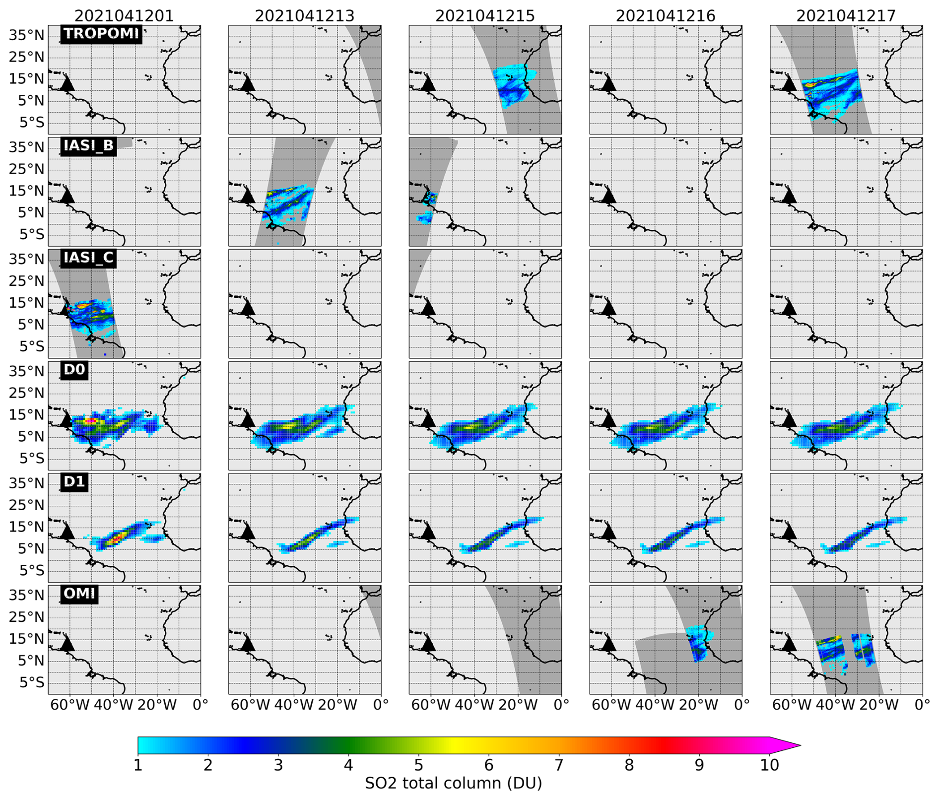
Figure 9 Observations and forecasts of SO₂ total columns on 12 April 2021 at 01:00, 13:00, 15:00, 16:00 and 17:00 UTC. The first row and the last row correspond to TROPOMI and OMI observations respectively. Forecasts are computed from the 11 April analysis outputs (second row) and from the 10 April analysis outputs (third row). These forecasts are available for 12 April.

Figure 10 represents the number of grid cells exceeding 1 and 5 DU for the D0 forecast in blue, for the D1 forecast in red and for the D2 forecast in green. The number of grid cells exceeding these thresholds is computed for TROPOMI in orange, IASI B in purple, IASI C in magenta and OMI in grey. We looked at the number of grid cells where the minimum and maximum of the total columns exceed these thresholds. These values are represented by horizontal lines in Fig. 10. The number of grid cells where the median of the observations exceeds these thresholds is shown as a dot. Finally, the limits of the bars represent the number of grid cells where the 25th and 75th quantiles exceed the thresholds.

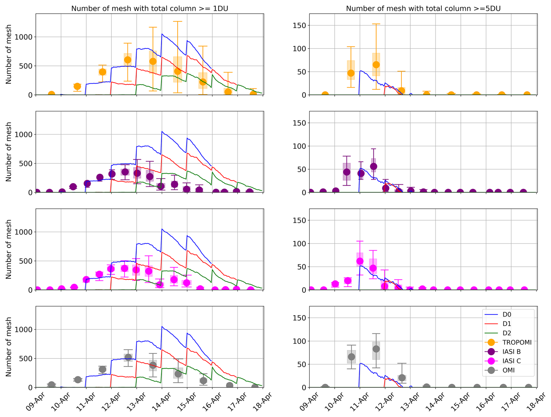
Figure 10 Number of grid cells where forecasts initialised by the joint_assim outputs reach 1 and 5 DU. The blue, red and green lines show the number of points at which the total columns reach these thresholds in the D0, D1 and D2 forecasts. Orange, purple, magenta and grey boxplots represent the number of grid cells where TROPOMI, IASI B, IASI C and OMI observations exceed the threshold.

Generally speaking, the number of meshes exceeding 1 or 5 DU decreases with the forecast period. This was not observed on 9 and 10 April, when no mesh exceeded 1 DU. The D0, D1 and D2 forecasts show the presence of a plume from 11, 12 and 13 April 2021. These forecasts are initialised by the output of the assimilation of 9 April, i.e. before the beginning of the eruption. On 11 April, there were around 200 grid cells where the model exceeded 1 DU for the D0 forecast. This number corresponds to the minimum number of grid cells where the TROPOMI and OMI observations reach 1 DU and is below the number of grid cells where the median of the IASI observations reaches 1 DU. On 12 April, the plume forecast with D0 was larger, with around 500 meshes exceeding 1 DU, corresponding to the number of meshes where the 25th quantile of the TROPOMI observations reached 1 DU and also where the median of the OMI observations reached this threshold. After this date, the number of occurrences of the SO₂ total column exceeding 1 DU increases and becomes greater than the number of grid cells where the IASI and OMI observations reach 1 DU. However, this number remains smaller than the maximum number of meshes calculated using TROPOMI observations. The number of points where the total column reaches 1 DU decreases with the forecast term range. Nevertheless, this number always exceeds the number of grid cells where the OMI and IASI observations reach 1 DU from 14 April onwards. Regarding the 5 DU threshold, no grid cell exceeds this threshold for the D2 forecast. The D1 forecast shows a low number on 12 April when the total columns reach 5 DU. However, this number is similar to the number of grid cells where the median of TROPOMI and IASI observations reaches 5 DU. In addition, for this day, the number of points where the model reaches 5 DU is similar between the D0 and D1 forecasts. For 11 April, the number of occurrences of a total column greater than or equal to 5 DU is low in the model compared with the UV instruments. This number is within the range of grid cells where IASI observations exceed 5 DU.

Figure 11 represents the POD (on the first line), the CSI (on the second line) and the FAR (on the third line) metrics calculated by comparing the observations measured by OMI and the forecasts at several time steps for 1 and 5 DU thresholds. The first forecast is launched on 9 April. Consequently, there is no D1 forecast available for this day and no D2 forecast available on 9 and 10 April. The last forecast is launched on 15 April, so there is no D0 forecast available on 16 and 17 April. There is no D1 forecast available on 17 April. For the POD and CSI metrics computed for the 1 DU threshold, the best values are found in the D0 forecast except on 14 and 15 April for the CSI metric. On 14 April CSI values are similar between the D0 and D1 forecast and on 15 April, the CSI is slightly better in the D2 forecast. Compared to POD values, CSI values are much lower, especially with D0 forecasts on 13 and 14 April. It means that there are a lot of locations where MOCAGE wrongly simulated total columns greater than 1 DU. This finding is strengthened by the presence of the highest FAR values during these days. The POD and CSI metrics computed with a 5 DU threshold show similar values. These metrics are 0 except on 11 April, with values around 0.2 for both the POD and CSI metrics. On 12 April both misses and false alarms occur with the D0 and D1 forecasts. Elsewhere, no SO₂ total columns greater than 5 DU are modelled and no observations greater than this threshold are observed by OMI on 14, 15 and 17 April. With the 5 DU threshold, there are only correct rejections.

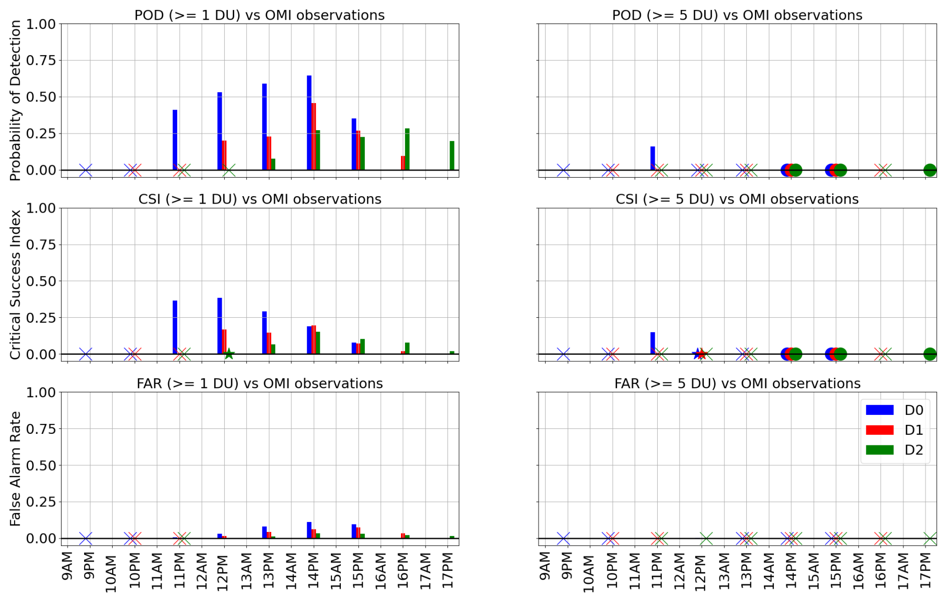
Figure 11 POD on the first line, CSI on the second line and FAR on the last line for the 1 and 5 DU thresholds for the D0 forecast in blue, the D1 forecast in red and the D2 forecast in green. The meaning of the symbols is described in Table 2.

Incorporating SO₂ total column analysis outputs into the MOCAGE forecasts enhances its ability to model an SO₂ plume. In the absence of the assimilation, the model fails to forecast the presence of an SO₂ plume. The use of recent analysis outputs progressively aligns the predicted location of the plume with the observations. However, the predicted intensity of the plume remains subject to high uncertainty.

7 Conclusion and perspectives

In this paper, we study the input of the assimilation of volcanic SO₂ total columns from TROPOMI, IASI, and both TROPOMI and IASI into the CTM MOCAGE in the case of the La Soufrière Saint Vincent eruption between 9 and 15 April 2021. For the background error covariance matrix, we used a profile containing high values in the volcanic plume vertical range extension. We considered a plume ranging from 9 to 21 km, corresponding to 90 % of the SO₂ plume heights diagnosed by the TROPOMI Layer Height product.

Thanks to the assimilation of TROPOMI and IASI data, an SO₂ plume is simulated in MOCAGE. This plume is modelled more or less early and corrected more or less often, depending on the time of the satellite overpass and on the instrument technology. The assimilation of both TROPOMI and IASI leads to a larger plume and a more realistic amount of SO₂ in the model. During this eruption, MOCAGE is able to simulate the process of converting SO₂ into sulfate aerosols. A sulfate plume, stronger by assimilating only TROPOMI, is computed by MOCAGE. With this creation of sulfate aerosols, AOD increases slightly. Nevertheless, few AOD observations are available during the studied period. Compared with SO₂ total columns observations, the number of pixels larger than 1 DU in the model is too large but the probability of detecting an SO₂ total column is important. In the model, the number of points with a total column greater than 5 DU is close to the number of grid cells with a median observation greater than 5 DU, especially when IASI and TROPOMI are assimilated. Compared to independent observations from OMI, the probability of detecting values greater than 5 DU is better when assimilating observations from both instruments.

Using assimilation outputs to compute forecasts improves the representation of SO₂ total columns in the model. The size and the shape of the plume depends on the forecast range term. As the forecast time range increases, the size of the plume decreases. Sometimes and especially for low values of the SO₂ total column, the size of the modelling plume is too large compared to the observations. Concerning the probability of detecting an SO₂ total column greater than a threshold, it is generally better for the short-term forecast.

One potential source of discrepancy is the assumptions regarding the altitude and thickness of the plume, which are dynamic in space and time. An inaccurate representation of the SO₂ plume height within the model could lead to a more dispersed plume or, depending on wind shear conditions, could result in the plume drifting in an incorrect direction. To refine our assimilation process, we could incorporate observed volcanic SO₂ plume heights from both IASI and TROPOMI. This approach, as suggested by Inness et al. (2022), would likely yield a more accurate simulation of the altitude of the plume, thereby producing a modelled plume shape that better reflects reality.

Another factor contributing to the overestimation of the plume extent within the MOCAGE model is the assimilation settings. Specifically, the application of an excessively large horizontal and vertical correlation length could lead to too extended a plume both on the vertical and the horizontal dimensions. Moreover, the chosen standard deviation for the background error can significantly influence the simulated intensity of the plume. With too large a value, the SO₂ plume concentration can be underestimated in MOCAGE, whereas with too small a value, the plume intensity can be too strong.

Additionally, inherent uncertainties in the model itself must be considered. The chemical processes involving SO₂, including reactions that may not be fully captured, introduce additional complexity into the simulation (Schumann et al., 2011). Furthermore, the meteorological data driving the model are not without their uncertainties (Webster and Thomson, 2022), which can compound the challenges in accurately modelling the transport and transformation of SO₂ emissions.

Satellites can give information on the locations where no SO₂ is detected. The use of this information for the assimilation could improve the process because it allows for limiting the shape of the plume.

To facilitate the assimilation of the SO₂, particularly the convergence of the minimiser, we could also use a prior volcanic SO₂ emission. In fact, the model and the observations are very different, sometimes by several orders of magnitude. To estimate volcanic SO₂ emissions, a source inversion of the volcanic SO₂ could be used (Boichu et al., 2013).

We also have seen that the more frequently the model is corrected, the closer it is to the observations. Assimilating additional instruments would therefore improve assimilation of the SO₂. The best option would be to assimilate observations from geostationary satellites covering the globe.

Finally, we made a specific adjustment for this eruption. Ideally, we would like to have a task running daily with assimilation settings that would allow us to assimilate the volcanic SO₂ for each eruption.