Exploring dual-lidar mean and turbulence measurements over Perdigão's complex terrain

To assess the accuracy of lidars in measuring mean wind speed and turbulence at large distances above the ground as an alternative to tall and expensive meteorological towers, we evaluated three dual-lidar measurements in virtual-mast (VM) mode over the complex terrain of the Perdigão-2017 campaign. The VMs were obtained by overlapping two coordinated range height indicator scans, prioritising continuous vertical measurements at multiple heights at the expense of high temporal and spatial synchronisation. Forty-six days of results from three VMs (VM1 on the SW ridge, VM2 in the valley, and VM3 on the NE ridge) were compared against sonic readings (at 80 and 100 m a.g.l.) in terms of 10 min means and variances to assess accuracy and the influence of atmospheric stability, vertical velocity, and sampling rate on VM measurements. For mean flow quantities – wind speed (V_h) and u and v velocity components – the r² values were close to 1 at all VMs, with the lowest equal to 0.948, whereas in the case of turbulence measurements ($u^{\prime }{u}^{\prime }$ and $v^{\prime }{v}^{\prime }$), the lowest was 0.809. Concerning differences between ridge and valley measurements, the average RMSE for the wind variances was 0.295 m² s⁻² at the VMs on the ridges. In the valley, under a more complex and turbulent flow, smaller between-beam angle, and lower lidars' synchronisation, VM2 presented the highest variance RMSE, 0.600 m² s⁻² for $u^{\prime }{u}^{\prime }$. The impact of atmospheric stability on VM measurements also varied by location, especially for the turbulence variables. VM1 and VM3 exhibited better statistical metrics of the mean and turbulent wind under stable conditions, whereas at VM2, the better results with a stable atmosphere were restricted to the wind variances. We suspect that with a stable and less turbulent atmosphere, the scan synchronisation in the dual-lidar systems had a lower impact on the measurement accuracy. The impact of the zero vertical velocity assumption on dual-lidar retrievals at 80 and 100 m a.g.l. in Perdigão was minimal, confirming the validity of the VM results at these heights. Lastly, the VMs' low sampling rate contributed to 33 % of the overall RMSE for mean quantities and 78 % for variances at 100 m a.g.l., under the assumption of a linear influence of the sampling rate on the dual-lidar error. Overall, the VM results showed the ability of this measurement methodology to capture mean and turbulent wind characteristics under different flow conditions and over mountainous terrain. Upon appraisal of the VM accuracy based on sonic anemometer measurements at 80 and 100 m a.g.l., we obtained vertical profiles of the wind up to 430 m a.g.l. To ensure dual-lidar measurement reliability, we recommend a 90° angle between beams and a sampling rate of at least 0.05 Hz for mean and 0.2 Hz for turbulent flow variables.

1 Introduction

To evaluate the wind at higher heights (>100 m), measurements from equipment other than anemometric towers are usually employed, as the costs associated with the installation and maintenance of masts scale with height. An alternative to the use of towers at great heights is the wind lidar.

Lidars measure the wind radial velocity up to kilometres of distance, and when employing a single lidar, a homogeneous flow assumption is needed to retrieve the wind vector components. However, under complex wind flow, this may not be a valid assumption, and measurements may present high systematic errors and inaccurate turbulence parameter estimations (Bingöl et al., 2009a, b; Sathe et al., 2011; Pauscher et al., 2016). For turbulence measurements, relevant to wind turbine load calculations, lidar retrievals are susceptible to cross-contamination and volume-averaging errors (Davies et al., 2005).

To reduce wind measurement uncertainty when using a single lidar in complex terrain, some authors have employed wind models to correct for flow distortion in profiling lidar measurements (Pitter et al., 2012; Klaas et al., 2015; Kim and Meissner, 2017). This approach, however, highly depends on the model's configurations and parameterisations (Klaas et al., 2015).

A more reliable solution to a single lidar is using two or more lidars configured to measure the same control volume simultaneously. In the case of three lidars, the three wind vector components can be retrieved from the radial velocities and azimuth and elevation angles (Mann et al., 2008; Sjöholm et al., 2009; Choukulkar et al., 2017). When two lidars are employed, one wind component, such as the vertical velocity, is assumed to be zero, and the other two are estimated. However, a multi-lidar approach implies high equipment costs and difficulties in coordinating and synchronising the lidar beams (Vasiljević et al., 2016). The scan strategy when employing multi-lidars can vary according to the study's objective. Triple-lidar setups were used by Wildmann et al. (2018) to investigate wind turbine wake and by Newman et al. (2016) to assess turbulence measurements. Coplanar range height indicator (RHI) scans were employed to evaluate rotor structures in a valley by Hill et al. (2010), while Calhoun et al. (2006) overlapped RHI scans to retrieve horizontal wind speed profiles in an urban site.

The association of at least two non-collocated lidars measuring multiple heights in a vertical line is called a virtual mast (VM) or virtual tower. Lidars can be configured with stop-and-stare (Damian et al., 2014; Pauscher et al., 2016; Newman et al., 2016; Debnath et al., 2017b; Wittkamp et al., 2021; Liu et al., 2024) or RHI scans (Calhoun et al., 2006; Ng and Hon, 2022; Newsom et al., 2005; Debnath et al., 2017a). Usually, the stop-and-stare scan has a higher spatial and temporal synchronisation but needs more time to measure at different heights as the equipment accelerates and decelerates from one measurement height to the next. Conversely, continuous vertical measurements of overlapping RHIs cover several heights more quickly, although usually with less accuracy, due to the scans not being entirely temporally and spatially synchronised, which is mainly a problem in an unstable atmosphere (Wittkamp et al., 2021; Choukulkar et al., 2017).

Rothermel et al. (1985) were the first to assess the feasibility of the dual-lidar methodology. Recent studies include experiments in complex terrain (Hill et al., 2010; Cherukuru et al., 2015; Santos et al., 2020; Duscha et al., 2023) and urban environments (Collier et al., 2005; Newsom et al., 2005; Calhoun et al., 2006; Wittkamp et al., 2021). The effect of atmospheric stability on virtual-mast measurements was evaluated by Newman et al. (2016) and Choukulkar et al. (2017) over flat terrains. Under stable atmospheric conditions, Newman et al. (2016) found that 10 min turbulent fluctuations from a triple-lidar VM setup aligned closely with Doppler beam swinging (DBS) (Strauch et al., 1984) estimations and diverged in an unstable atmosphere. However, the study did not include sonic measurements at the same height as the virtual mast, later addressed by Choukulkar et al. (2017), who evaluated triple-lidar VM mean measurements against mean sonic observations (at 50–300 m a.g.l., in 50 m increments). The VM results under stable conditions showed smaller errors than in an unstable atmosphere, which was attributed to the higher wind variability in unstable conditions, potentially leading to greater measurement uncertainty.

Despite previous efforts to evaluate multi-lidar measurements, no study has assessed the mean horizontal wind components obtained from two lidar-coordinated RHI scans in a VM mode, with reference sonic anemometer readings, or investigated second-order wind statistics from dual-lidar RHI retrievals or the influence of atmospheric stability and sampling rate on these data. Therefore, this study explores coordinated dual-lidar RHI measurements, in a VM mode, of the mean and turbulent flow under different wind conditions over Perdigão's complex terrain. The virtual-mast results are evaluated against sonic anemometer data at one or more matching heights in terms of coefficient of determination (r²) and statistical errors (RMSE and bias).

The VM measurements come from the Perdigão-2017 campaign (Fernando et al., 2019), a field experiment that was part of the New European Wind Atlas (NEWA) (Mann et al., 2017). During the campaign, profiler (8) and scanning (18) lidars were deployed (Fernando et al., 2019). The latter operated with different scanning schemes, including RHIs along the ridges, RHIs across the ridges (in three transects), and coordinated setups forming dual-lidar measurements. This work focuses on four virtual masts from the experiment, positioned in a transect almost perpendicular to Perdigão's double ridge and formed by seven WindScanners (WSs) – not previously analysed. Thus, we needed to assess the measurements' quality compared to reference data, develop a processing and filtering methodology, and explore the capabilities and limitations of these VMs in Perdigão.

The performance of WindScanners in dual and triple measurement setups, staring at a single point, was evaluated by Pauscher et al. (2016), who compared the results with a sonic anemometer (at 188 m a.g.l.) and DBS readings. The study focused on first- and second-order statistics of horizontal wind components measured by three dual-lidar configurations and one triple-lidar configuration. However, the analysis was limited to a single point, correlating the WS measurements without error quantification.

Previous virtual-mast-based studies in Perdigão combined scanning lidars at different positions than those examined here and with a different focus. Bell et al. (2020) evaluated RHI dual- and triple-lidar measurements in four locations along the Perdigão valley in a VM mode (from 50–600 m a.g.l.), focusing on the analysis of the valley flow. However, since the lidars were not coordinated, the VM analysis was based on 15 min mean values, and a time window of 60 s between lidar scans was imposed, which restricted the result analysis to only mean quantities. Triple-lidar VM measurements at different distances within Perdigão's wind turbine wake were investigated by Wildmann et al. (2019), who proposed a new approach to retrieve the turbulence dissipation rate from RHI lidar retrievals.

Beyond the difficulties in multi-lidar measurements, an additional one lies in measuring the complex wind flow above the mountainous terrain of Perdigão. With wind turbines increasingly being placed in complex terrains due to the depletion of flatland and more site constraints, a greater understanding and mapping of the wind in such areas are required. Furthermore, with the growth in height and rotor of modern wind turbines, it is crucial to assess the wind potential and characteristics at greater heights.

2 The campaign and equipment

2.1 Field campaign

Located in Portugal's mainland, the Perdigão site is characterised by two parallel ridges (SW and NE) with an elevation of about 250 m above the nearby terrain, separated by 1.4 km, and extending over 4 km (Fig. 1). The SW ridge averages 231.2 m, with a slope of around 33.3°; the NE ridge is about 217.6 m, with an inclination of 28.5°; and the valley floor is 41.9 m. The terrain coverage is non-homogeneous, with a mixture of low vegetation and eucalyptus and pine tree patches (Palma et al., 2020).

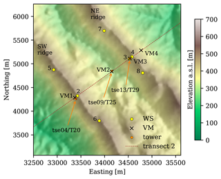
Figure 1 Perdigão terrain (Farr et al., 2007) and measuring device locations (ETRS89/PT-TM06).

Table 1 Coordinates and elevation of each measurement source.

In the Perdigão-2017 campaign, multiple measuring devices worked simultaneously to obtain a high-resolution dataset from 1 May until 15 June 2017. This is called the intensive observational period (IOP) and is the study period of this work. Among the installed equipment, the sensors employed here are those installed in the three 100 m masts and seven WindScanners operated by the Technical University of Denmark (DTU; Fig. 1).

The wind flow in Perdigão was initially assumed to be two-dimensional, with the predominant wind direction perpendicular to its double ridge (Fernando et al., 2019). However, the measurements revealed Perdigão's intricate wind flow. Despite the uniform perpendicular flow on the synoptic scale, on smaller scales, the wind exhibits two main directions (Fig. 2). In the valley, the wind direction aligns with the valley (tse09/T25 wind rose), while on the ridges (tse04/T20 and tse13/T29 wind roses), it is perpendicular to the valley.

Figure 2 Wind roses of the 10 min averaged wind speed and direction from tse04/T20 (SW ridge), tse09/T25 (valley), and tse13/T29 (NE ridge) measurements at 100 m a.g.l. during the intensive observational period.

2.2 Towers

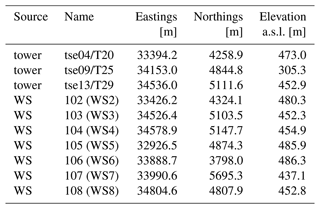
The three 100 m towers were located along transect 2 (Menke et al., 2019b), almost perpendicular to the ridges: tse04/T20 on the SW ridge, tse09/T25 in the valley, and tse13/T29 on the NE ridge (Fig. 1 and Table 1). The tower equipment provided wind speed and temperature measurements that were used in this study to evaluate the VM wind speed retrievals and classify the atmospheric stability.

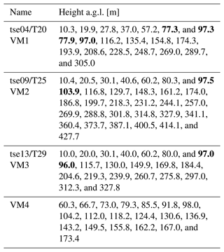
Gill 3D WindMaster Pro sonic anemometers were operated at a frequency of 20 Hz, with sensor heights shown in Table 3 and Fig. 3. NCAR SHT75 temperature and humidity sensors were installed at seven levels: 2, 10, 20, 40, 60, 80, and 100 m a.g.l. The post-processed (quality-controlled, tilt-corrected, and in a geographic coordinate system) data from these instruments were downloaded from UCAR/NCAR – Earth Observing Laboratory (2019a). The sonic anemometer data were tilt-corrected using laser survey measurements (Menke and Mann, 2017) to determine the azimuth, pitch, roll, and height of each anemometer, ensuring that the post-processed wind components were represented in geographical coordinates (UCAR/NCAR – Earth Observing Laboratory, 2019b).

2.3 WindScanners

Eight WindScanners (WS1–8), four on each ridge and operated by DTU (Vasiljević et al., 2016; Menke et al., 2019a), were employed in the Perdigão-2017 campaign. In terms of settings, the range gate separation (15 m), full width at half maximum of the spatial weighting function (30 m), spatial coverage (from 100 to 3000 m away from the equipment), elevation step (0.75°), accumulation time (500 ms), and pulse length (200 ns) were identical for all WindScanners. WS1–4, WS6, and WS8 had an elevation range of 36°, while WS5 and WS7 covered an angular range of 18°. WindScanners 1–4 performed RHI measurements along transect 2, and WindScanners 5–8 operated in a sequence of three scan types, each with a 10 min duration: along the ridge, virtual-mast, and transect scans. By crossing WS2–4 RHI measurements with WS5–8 virtual-mast scan (also RHI), four virtual masts (VM1–4) were reconstructed with the campaign measurements (Fig. 1 and Table 2).

To guarantee the quality of the WS measurements, before the dual-lidar processing, the WS data were initially filtered out according to the equipment's radial velocity limits ($[-\mathrm{30},\mathrm{30}]$ m s⁻¹) and the carrier-to-noise ratio (CNR), where a threshold equal to −22 dB (determined from CNR versus radial velocity plots of the multiple WindScanners) was imposed. The WS spectrum data were not stored in the Perdigão campaign; only the processed signal results were. Other filters were employed while processing the VM measurements (Sect. 3.1).

3 Virtual-mast retrieval

During the Perdigão-2017 experiment, four virtual masts (VM1–4) were configured (Menke et al., 2019a) according to the intersection point between two non-collocated WindScanners (WS_a and WS_b; Table 2). Two virtual masts (VM1 and VM3) were located on the top of the SW and NE ridges, another VM was located in the valley (VM2), and the last one was located downhill from the NE ridge (VM4; Fig. 1). VM1–3 were located at distances of 32.4, 9.4, and 3.3 m, respectively, from tse04/T20, tse09/T25, and tse13/T29 100 m towers to compare VM results with reference equipment at overlapping heights and to map the vertical profile of the wind from 10 to around 430 m a.g.l.

Table 2 Virtual-mast coordinates, lidar combinations, and range of elevation angles (ϕ).

3.1 Dual-lidar processing and filtering

The processing and filtering of the dual-lidar measurements in Perdigão required the following steps.

•  

  Step 1. The radial velocities of WS_a (${v_{\mathrm{r}}}_{\mathrm{a}}$) and WS_b (${v_{\mathrm{r}}}_{\mathrm{b}}$) were interpolated along the beam direction at the VM coordinates (Table 2).

•  

  Step 2. The VM heights (Table 3 and Fig. 3) were calculated as the average of the closest WS_a and WS_b measurement heights.

•  

  Step 3. Likewise, the VM measurement timestamps were determined by averaging the WS_a and WS_b nearest timestamps.

•  

  Step 4. The Cartesian velocity components in the x (u) and y directions (v) were obtained from the radial velocities (v_r) and the azimuth (θ) and elevation (ϕ) angles of WS_a and WS_b, assuming that the vertical wind component is zero (w=0), by

  $$\begin{array}{}\text{(1)}& \left[\begin{array}{c}u\\ v\end{array}\right]={\left[\begin{array}{cc}\sin \left({\mathit{\theta }}_{\mathrm{a}}\right)\cos \left({\mathit{\varphi }}_{\mathrm{a}}\right)& \cos \left({\mathit{\theta }}_{\mathrm{a}}\right)\cos \left({\mathit{\varphi }}_{\mathrm{a}}\right)\\ \sin \left({\mathit{\theta }}_{\mathrm{b}}\right)\cos \left({\mathit{\varphi }}_{\mathrm{b}}\right)& \cos \left({\mathit{\theta }}_{\mathrm{b}}\right)\cos \left({\mathit{\varphi }}_{\mathrm{b}}\right)\end{array}\right]}^{-\mathrm{1}}\left[\begin{array}{c}{v}_{r_{\mathrm{a}}}\\ v_{r_{\mathrm{b}}}\end{array}\right].\end{array}$$

  Subsequently, the horizontal wind speed (V_h) was calculated.

  • Averages and variances of wind velocity components and wind speed were calculated within 10 min intervals.

•  

  Step 5. The VM measurements were filtered in two steps.

  • The first filter aimed to eliminate hard target interference in VM measurements (Sect. 3.1.1).

  • The second filter identified the VM minimum quantity of measurements (MQM) within 10 min intervals (Sect. 3.1.2).

Table 3 Measurement heights (matching heights between the nearby tower and the VM are in bold).

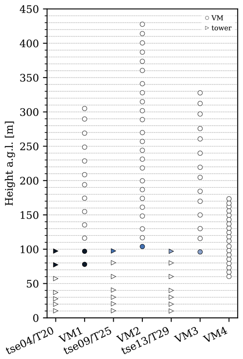
Figure 3 Tower and VM heights of wind speed measurements (matching heights in coloured markers: dark blue for tse04/T20 and VM1, medium blue for tse09/T25 and VM2, and light blue for tse13/T29).

After these processing steps, we ended up with dual-lidar measurements that spanned the atmosphere from 80 to 305 m a.g.l. in VM1, 100 to 430 m in VM2, 100 to 330 m in VM3, and 60 to 170 m in VM4 – i.e. more than 4 times the height of conventional tall meteorological towers (100 m a.g.l.). We focused our analysis on the measurements from VM1 at 80 and 100 m, VM2 at 100 m, and VM3 at 100 m, as these were the only measurements obtained at the same height as the sonic anemometer readings, enabling the evaluation of the VM data's reliability.

Upon validating their accuracy, we can use the entire VM dataset in further studies. However, at higher heights, the assumption of zero vertical velocity (Step 4) can reduce the accuracy of the horizontal wind components obtained from dual-lidar measurements, since the increase in beam elevation angles causes the lidar beams to be more aligned with the vertical component of the wind.

3.1.1 Hard target filter

Some WS measurements had interference from hard targets, such as terrain, vegetation, and masts, and were, therefore, filtered out. As a result, VM2 and VM3 presented only one measuring height that overlapped with the sonic heights, at around 100 m a.g.l., while VM1 had two measuring heights that matched the tse04/T20 sonics, at ∼ 80 m and ∼ 100 m a.g.l.

3.1.2 Minimum quantity of measurement filter

Although the WSs were configured to perform approximately 22 VM scans in each 10 min measurement period, device restrictions and filtering led to periods with fewer valid scans, as shown in Fig. 4 for VMs' measurements at 100 m a.g.l. To evaluate the impact of the number of valid scans per 10 min period on VM measurement accuracy, we computed error indicators for VM1–3 datasets under various filtering thresholds (Table 4). Starting with unfiltered data (0 % filter), we defined the minimum number of scans (threshold) required for a 10 min measurement to be considered valid, progressively increasing the filter criteria (as represented by the percentage values in Table 4) up to a 90 % filter. For example, with the 20 % filter, a 10 min measurement was considered valid and included in the analysis if it contained at least 20 % of the total scan quantity, i.e. four valid scans for a maximum of 22.

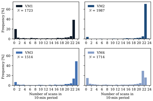
Figure 4 Histogram of the number of valid scans in 10 min periods for all virtual masts at ∼ 100 m a.g.l., before the MQM filter. N represents the total number of valid 10 min measurements at ∼ 100 m a.g.l. during the IOP, before the MQM filter.

Table 4 Errors between VMs and towers according to the minimum quantity of measurements (MQM) in 10 min periods for u, v, $u^{\prime }{u}^{\prime }$, and $v^{\prime }{v}^{\prime }$.

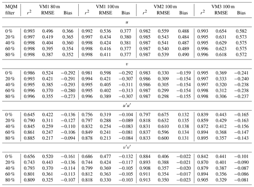
The RMSE and bias units are m s⁻¹ for u and v variables, while for $u^{\prime }{u}^{\prime }$ and $v^{\prime }{v}^{\prime }$ the units are m² s⁻². r² is unitless.

The turbulence measurements ($u^{\prime }{u}^{\prime }$ and $v^{\prime }{v}^{\prime }$) were more sensitive to the MQM filter than the mean values (u and v), as evidenced mainly by the RMSE (Table 4). Consequently, this metric was chosen as the criterion for identifying the optimal MQM filter value, which retrieves a VM dataset with low errors while avoiding a significant data loss, caused by a too-constrained filter.

The balance between low RMSE and low data loss occurs when $\mathrm{\Delta }\mathrm{RMSE}/\mathrm{\Delta }N\approx \mathrm{1}$. Here, ΔRMSE is the percentage difference in RMSE between any MQM filter above 0 % and the raw data (0 % filter), and ΔN is the percentage difference in the number of samples between the two datasets. By averaging $\mathrm{\Delta }\mathrm{RMSE}/\mathrm{\Delta }N$ across all VMs, we determined that the optimal MQM filter is 50 % for the mean and 80 % for the turbulence VM measurements. Applying a filter higher than 50 % (80 %) can reduce the dataset size to a point where the remaining data become less representative of the mean (turbulent) wind flow. Therefore, subsequent mean and turbulence results will be presented using 50 % and 80 % MQM filters.

Since VM4 is the only virtual mast with no reference measurement nearby, the filtering procedure determined through the VM1–3 analysis was replicated at VM4.

3.2 Dual-lidar measurement constraints and error sources

As two simultaneous WSs are required to produce a VM measurement, the VM is constrained by the availability of both WindScanners. WS2–4 (WS_a in Table 2) continuously performed RHI scans, while WS5–8 (WS_b in Table 2) only did the intercepting RHI scan twice per hour. Thus, the VM measurements occurred twice per hour within 10 min. During the 10 min period, each WS performed a maximum of 22 or 23 scans (Fig. 4); i.e. a maximum sampling rate of 0.038 Hz ($\mathrm{23}/\mathrm{600}$ Hz), approximately 500 times lower than the sonic anemometer frequency (equal to 20 Hz).

Another constraint was the dependence of VM data availability on concurrent measurements from both WindScanners, which, at specific periods, depicted limited data due to equipment downtime or filtering (low CNR, hard targets, and MQM filter). The data availability for each VM at 100 m a.g.l. during the IOP is detailed in Table 5. For mean wind components, the average data availability for all heights was 46.2 % for VM1, 76.3 % for VM2, 54.1 % for VM3, and 56.9 % for VM4. For $u^{\prime }{u}^{\prime }$ and $v^{\prime }{v}^{\prime }$, on the other hand, availability was 37.5 %, 69.8 %, 47.8 %, and 49.2 % for VM1–4.

Table 5 Data availability of the VM measurements at 100 m a.g.l. during the IOP.

The interception angle (Δχ) between lidars' beams (Table 6), with directions ${\widehat{\mathbf{r}}}_{\mathrm{a}}$ and ${\widehat{\mathbf{r}}}_{\mathrm{b}}$, influences the accuracy of VM results. This is because the dual-lidar error of a retrieved wind field component (σ_DD(u_j)) is (Stawiarski et al., 2013)

$$\begin{array}{}\text{(2)}& \begin{array}{rl}& {\mathit{\sigma }}_{\mathrm{DD}}\left(u_j\right)=\\ & {\left[{\displaystyle \frac{{\sin }^{\mathrm{2}}({\mathit{\alpha }}_j+\mathrm{\Delta }\mathit{\chi }/\mathrm{2})+{\sin }^{\mathrm{2}}({\mathit{\alpha }}_j-\mathrm{\Delta }\mathit{\chi }/\mathrm{2})}{{\sin }^{\mathrm{2}}\mathrm{\Delta }\mathit{\chi }}}\right]}^{\mathrm{1}/\mathrm{2}}{\mathit{\sigma }}_{v_{\mathrm{r}}},\end{array}\end{array}$$

where ${\left[\frac{{\sin }^{\mathrm{2}}({\mathit{\alpha }}_j+\mathrm{\Delta }\mathit{\chi }/\mathrm{2})+{\sin }^{\mathrm{2}}({\mathit{\alpha }}_j-\mathrm{\Delta }\mathit{\chi }/\mathrm{2})}{{\sin }^{\mathrm{2}}\mathrm{\Delta }\mathit{\chi }}\right]}^{\mathrm{1}/\mathrm{2}}$ is the error prefactor, α_j is the angle between the direction of the wind field component (${\widehat{\mathbf{e}}}_j$) and the mean lidar direction (${\widehat{\mathbf{r}}}_m=({\widehat{\mathbf{r}}}_{\mathrm{a}}+{\widehat{\mathbf{r}}}_{\mathrm{b}})/\mathrm{2}$), and ${\mathit{\sigma }}_{v_{\mathrm{r}}}$ is the radial velocity error, assuming that is identical in both lidars (${\mathit{\sigma }}_{v_{\mathrm{r}}}={\mathit{\sigma }}_{v_{\mathrm{r}}}^{\mathrm{a}}={\mathit{\sigma }}_{v_{\mathrm{r}}}^{\mathrm{b}}$). While the radial velocity error depends on several factors, such as the specific lidar, atmospheric backscatter, distance from the instrument, focus position, and instrument temperature, we assume it to be identical in both lidars because the angle between the beams is a more significant contributor to the dual-lidar error.

Table 6 Average angle between lidars' beams (Δχ) and prefactors of the dual-lidar propagation error for the horizontal velocity components (u and v).

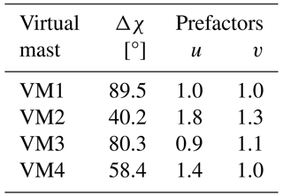
The prefactor is directly influenced by the between-beam angle and the direction of the wind component, namely u and v, and indirectly by the VM height (Fig. 5), as Δχ varies with the beams' elevation angles. Ideally, the angle between the beams would be close to 90°, which results in prefactors equal to 1, regardless of the wind component direction. At Perdigão's four virtual masts, only VM1 and VM3 had Δχ close to the optimal angle (∼ 89.5 and ∼ 80.3°), while the angles at VM2 and VM4 were 40.2 and 58.4°, on average (Table 6). This means that the prefactors and the propagation of the radial velocity error at VM2 and VM4 are greater than at VM1 and VM3.

When retrieving the u velocity, the dual-lidar propagation error is about 1.0, 1.8, 0.9, and 1.4 times the error of the radial velocity for VM1–4, respectively (Table 6). For the v velocity, the prefactors are around 1.0, 1.3, 1.1, and 1.0 for VM1–4. On the other hand, the dual-lidar error of the horizontal wind speed is a combination of the σ_DD(u), σ_DD(v), and wind speed components:

$$\begin{array}{}\text{(3)}& \begin{array}{rl}& {\mathit{\sigma }}_{\mathrm{DD}}\left(V_{\mathrm{h}}\right)=\\ & {\left[{\left({\displaystyle \frac{u}{\sqrt{u^{\mathrm{2}}+v^{\mathrm{2}}}}}{\mathit{\sigma }}_{\mathrm{DD}}\left(u\right)\right)}^{\mathrm{2}}+{\left({\displaystyle \frac{v}{\sqrt{u^{\mathrm{2}}+v^{\mathrm{2}}}}}{\mathit{\sigma }}_{\mathrm{DD}}\left(v\right)\right)}^{\mathrm{2}}\right]}^{\mathrm{1}/\mathrm{2}},\end{array}\end{array}$$

assuming that the errors in u and v are not correlated.

With regard to height variation (Fig. 5), the prefactors varied little and generally showed higher values with increasing height, except for the v wind component measured by VM1.

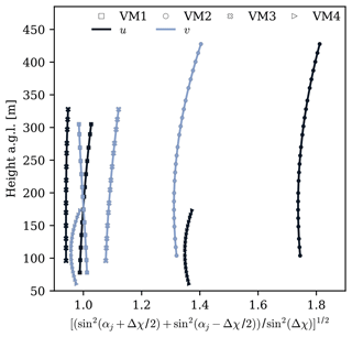
Figure 5 Dual-lidar error prefactor $\left[\right({\sin }^{\mathrm{2}}({\mathit{\alpha }}_j+\mathrm{\Delta }\mathit{\chi }/\mathrm{2})+{\sin }^{\mathrm{2}}({\mathit{\alpha }}_j-\mathrm{\Delta }\mathit{\chi }/\mathrm{2}))/{\sin }^{\mathrm{2}}(\mathrm{\Delta }\mathit{\chi }){]}^{\mathrm{1}/\mathrm{2}}$of a retrieved wind field component as a function of the beam height for VM1–4.

Another source of error when combining radial velocities from different lidars can arise when there is a mismatch in their range gate heights (Stawiarski et al., 2013). Such mismatch can cause the lidars to measure different wind structures, mainly under high-vertical-wind-shear conditions. For the Perdigão-2017 campaign, the height difference between the range gate centers, after the radial interpolation, varied for each height and virtual mast. At VM1–4, the displacements went up to 4.4, 6.8, 8.7, and 1.6 m, respectively. However, given that the spatial resolution of the WindScanners was approximately 30 m, this mismatch is not expected to impact the virtual-mast results substantially.

In addition, the lidars' scans were not fully synchronised in time (Fig. 6). This means that measurements from WS_a and WS_b occurred at slightly different times, which can lead to time-average errors in the dual-lidar measurements (Stawiarski et al., 2013) due to the stationary atmospheric assumption (Choukulkar et al., 2017). At VM1, the predominant time differences between WS_a and WS_b ranged from 0 to 2 s, accounting for 53.7 % of all VM1 measurements. At VM2, WS_b consistently recorded measurements later than WS_a, leading to time lags of 8–10 s in 69.8 % of VM2's measurements. For VM3, 51.1 % of the measurements depicted a time difference between 3 and 5 s. Meanwhile, at VM4, the time difference for 62.8 % of the measurements fell in the [1 s, 3 s) interval. While these desynchronisations may impact the retrieval of turbulent variables, their influence is expected to be insignificant for mean quantities.

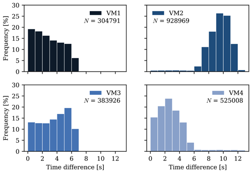
Figure 6 Time difference histogram of the mean flow measurements at all heights between the lidars constituting the virtual masts. N represents the total number of valid 10 min measurements at all heights during the IOP.

Lastly, the horizontal position of each VM differed from the corresponding tower locations. This can affect the VM results when nearby tower measurements are used as a reference due to the underlying assumption of a spatially homogeneous atmosphere. This is most pronounced for VM1, located 32.4 m apart from tse04/T20. Meanwhile, VM2 was 9.4 m from tse09/T25, and VM3 was 3.3 m from tse13/T29.

4 Results and discussion

This section compares virtual-mast and sonic measurements and how atmospheric stability, vertical velocity, and sampling rate influence the VM wind velocity and turbulence retrievals. The analyses are based on 10 min averages of the horizontal wind speed (V_h) and its components (u and v), as well as their variances ($u^{\prime }{u}^{\prime }$ and $v^{\prime }{v}^{\prime }$). The virtual-mast and sonic comparisons also cover radial velocity means (v_r) and variances (${v_{\mathrm{r}}}^{\prime }{v_{\mathrm{r}}}^{\prime }$). All results are in local time, equal to UTC + 1 h in the summer period, and in the ETRS89/PT-TM06 coordinate system.

4.1 Virtual-mast and sonic comparisons

Virtual-mast and tower measurements were compared at their closest heights, with no vertical interpolation: VM1 at 77.9 and 97.0 m with tse04/T20 at 77.3 and 97.3 m, VM2 at 103.9 m with tse09/T25 at 97.5 m, and VM3 at 96.0 m with tse13/T29 at 97.0 m. For simplification, the comparison heights were rounded to 80 and 100 m.

As a first analysis, $v_{r_{\mathrm{a}}}$ and $v_{r_{\mathrm{b}}}$ from the WindScanners of VM1–3 were compared against sonic measurements projected in the laser beam direction to assess the measurements of each WS equipment without introducing uncertainties related to the dual-lidar methodology (Sect. 3).

Care must be taken when comparing VM results in the valley (VM2) with those on the ridges (VM1 and VM3), since the flows are intrinsically different at the comparison heights (80 and 100 m a.g.l.). In the valley, the main wind direction is along the valley, whereas on the ridges the main wind direction is cross-valley; the wind speeds are lower (Fig. 2); and the turbulence intensity is 2.7 times higher than on the ridges.

4.1.1 Mean flow measurements

In the comparison between VM and sonic v_r (Table 7), the fit of the linear regressions for all WindScanners was almost perfect, with r² values close to 1. The lowest r² was equal to 0.989 (WS6 at VM2 100 m). In the linear regression equation ($y=mx+b$), despite the coefficients (m) being approximately 1, the constants (b), determined by where the line intercepts the y axis, assumed positive (WS5, WS2, and WS7) and negative (WS3 and WS6) values according to the WS, meaning an overall overestimation and underestimation of v_r. In addition, b values higher than 0.4 m s⁻¹ were observed in WS5 (0.414 m s⁻¹ at 80 m and 0.445 m s⁻¹ at 100 m a.g.l.) and WS7 (0.492 m s⁻¹ at 100 m a.g.l.). These WindScanners also showed higher RMSE and bias errors in their radial velocities at 100 m: 0.509 m s⁻¹ and 0.436 m s⁻¹ in WS5 and 0.586 m s⁻¹ and 0.523 m s⁻¹ in WS7.

Table 7 Statistical parameters from VM and tower comparisons for mean and variance variables.

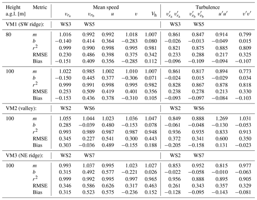
The units of b, RMSE, and bias are m s⁻¹ for mean variables and m² s⁻² for variances. m and r² are unitless. m is the coefficient, and b is the constant of the linear regression equation ($y=mx+b$).

When WS5 and WS7 form VM1 and VM3, their beams align with the direction of the ridges (Fig. 1), and at the top of the hills, the main wind directions are perpendicular to the ridge's orientation (Fig. 2). Thus, due to a lidar's inherent limitation to directly measure the wind component perpendicular to its beam orientation, WS5 and WS7 setups contribute to their wind speed measurement errors.

For the horizontal wind speed (V_h) and u and v wind components obtained from the dual lidars, besides the beam orientation of each WS regarding the position of the wind, the intersection angle between the two beams is also important (Table 6). At VM1 and VM3, Δχ was close to 90°, the optimal angle to retrieve u and v, whereas at VM2, the angle was about 40°, yielding higher dual-lidar propagation error in the u and v components, with mean prefactors equal to 1.8 and 1.3 (Table 6 and Fig. 5).

The coefficients of determination were close to 1 for the mean wind variables at all virtual masts (Table 7 and Fig. 7), with the lowest values equal to 0.987 for u and v and 0.948 for V_h at VM2. The lower r² values at VM2 are attributed to the smaller angle between WS2 and WS6 beams and to the turbulent flow in the valley, which may require a greater VM sampling rate than 0.038 Hz. The highest errors, however, occurred at VM3 for u (0.626 m s⁻¹ RMSE and 0.575 m s⁻¹ bias) and at VM1 for v (0.401 m s⁻¹ RMSE and −0.310 m s⁻¹ bias), while for the horizontal wind speed, VM3 obtained the highest RMSE, equal to 0.463 m s⁻¹, and VM2 the highest bias, 0.188 m s⁻¹. Additionally, all VM results overestimated the anemometer readings of the mean east–west wind component and V_h (positive bias), and they underestimated the north–south wind component (negative bias).

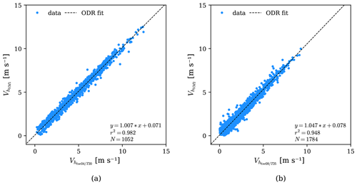
Figure 7 Mean flow measurements of virtual masts against sonic anemometer data: (a) VM1 and tse04/T20 V_h at 100 m a.g.l. and (b) VM2 and tse09/T25 V_h at 100 m a.g.l.

The average magnitude of the VM error (RMSE) did not follow the trend observed in the dual-lidar propagation errors. Contrary to the prefactor values (Table 6), VM2's u variable did not show the highest RMSE value among the VMs, and the x wind component in VM3 did not exhibit the lowest, indicating that factors beyond the error coefficient influenced the VMs' RMSE.

The V_h errors of the VMs generally fell within the range of those for the u and v components. The r², on the other hand, showed lower values (0.969 on average) than for u and v (0.994 on average).

Compared to Pauscher et al. (2016), the horizontal wind speed results of Perdigão's VMs showed lower r² values against reference sonic anemometer measurements, ∼ 3 % lower on average. The difference between both results is due to the scanning mode and the underlying assumptions in each scan. Pauscher et al. (2016) employed a staring configuration, recording data at 0.5 Hz, whereas in our analysis, the virtual-mast measurements were formed by combining two RHI scans with a maximum sampling rate of 0.038 Hz. In the latter, the lidar beams were constantly moving and not perfectly synchronised in time and space, resulting in a lower measurement frequency and forcing a greater flow homogeneity assumption compared to the staring approach.

4.1.2 Turbulence measurements

For the radial velocity variances ($v_{r_{\mathrm{a}}}^{\prime }{v}_{r_{\mathrm{a}}^{\prime }}$ and $v_{r_{\mathrm{b}}}^{\prime }{v}_{r_{\mathrm{b}}}^{\prime }$), the r² values were consistently lower than for the mean radial velocities (${v_r}_{\mathrm{a}}$ and $v_{r_{\mathrm{b}}}$), going from 0.994 in the means to 0.888 in the variances, on average (Table 7). The lowest coefficient of determination for ${v_r}^{\prime }{v_r}^{\prime }$ between lidar and sonic measurements was 0.821 at WS3 in VM1 80 m, whereas the highest was 0.956 at WS2 in VM3 100 m.

The radial velocity variance errors averaged 0.294 m² s⁻² for RMSE and −0.123 m² s⁻² for bias on the ridges. In the valley, under a more turbulent flow and with a low measurement rate, the average errors for ${v_{\mathrm{r}}}^{\prime }{v_{\mathrm{r}}}^{\prime }$ were higher than those on the ridges, with an RMSE of 0.357 m² s⁻² and bias of −0.182 m² s⁻². However, independent of the measurement location, all WindScanners underestimated the turbulence measurements (negative bias).

For $u^{\prime }{u}^{\prime }$ and $v^{\prime }{v}^{\prime }$, the VMs' low sampling rate led to a weaker linear correlation against sonic measurements than for u and v. The r² results, which were higher than 0.987 (VM2 u and v) for the mean wind speed components, assumed values as low as 0.809 (VM1 $v^{\prime }{v}^{\prime }$ at 80 m a.g.l.) in the variances (Table 7 and Fig. 8). This means the VM turbulence measurements did not portray the wind variability, represented by r², as the sonic anemometer readings and the VM averages.

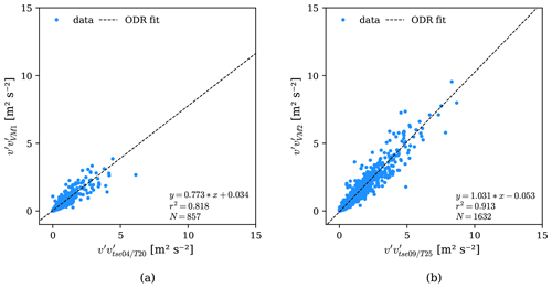
Figure 8 Turbulence measurements of virtual masts against sonic anemometer data: (a) VM1 and tse04/T20 $v^{\prime }{v}^{\prime }$ at 80 m a.g.l. and (b) VM2 and tse09/T25 $v^{\prime }{v}^{\prime }$ at 100 m a.g.l.

In the linear regression equation between VM and sonic turbulence measurements, b was close to zero in all VMs, with the highest value of −0.130 m² s⁻² for $u^{\prime }{u}^{\prime }$ at VM2, while the slope coefficient (m) ranged from 0.799 at 80 m VM1 ($v^{\prime }{v}^{\prime }$) to 1.269 at 100 m VM2 ($u^{\prime }{u}^{\prime }$). The steeper slope for VM2's turbulence measurements (both above 1) indicated greater sensitivity to changes in turbulence compared to the other VMs, where m was less than 1. However, this did not translate into better accuracy, as VM2 had the highest RMSE for turbulence measurements.

Regarding errors, on the ridges, the average RMSE for the turbulent wind components (0.295 m² s⁻²) was lower than in the valley (0.475 m² s⁻²), as also observed in the radial velocity results. The RMSE at VM2 for turbulence measurements was the highest (0.600 m² s⁻² for $u^{\prime }{u}^{\prime }$), while the highest bias was at VM3 (−0.143 m² s⁻² for $u^{\prime }{u}^{\prime }$), closely followed by VM2 (0.131 m² s⁻² for $u^{\prime }{u}^{\prime }$), in absolute values. The high errors in VM2 turbulence measurements are attributed to the approximately 9 s mismatch between the lidars. Other contributing factors are the small interception angle between the lidars' beams and the measurement sampling rate, which may be insufficient for the valley complex flow, as also observed in the VM2 mean flow results. Consistently with the distinct valley flow, $u^{\prime }{u}^{\prime }$ measured by VM2 uniquely overestimated the sonic measurements (positive bias), despite the negative bias in the radial velocity variances of WS2 and WS6.

Overall, the VM turbulence measurements showed a high mean r² value (0.867) and low mean errors (0.340 m² s⁻² RMSE and −0.063 m² s⁻² bias), despite the average r² being lower than that of the mean wind components (0.994), the imperfect synchronisation of the scans, and the low sampling rate. The relatively high accuracy of the VM results in capturing the turbulent flow, even with measurement constraints, indicates that in Perdigão, synoptic and mesoscale systems dominate the atmospheric circulation at the site, and small-scale phenomena played a minor role in the wind patterns.

In Pauscher et al. (2016), the r² values of $u^{\prime }{u}^{\prime }$ ($v^{\prime }{v}^{\prime }$) were equal to 0.954 (0.966), 0.887 (0.903), and 0.782 (0.861) for the three different dual-lidar combinations. On average, their r² values were ∼ 1 % (∼ 6 %) higher than the ones depicted here. This difference is again related to the nature of the scans (staring versus RHI combination), which affects the temporal–spatial synchronisation and the measurement frequency.

4.2 Influences on the dual-lidar results

Besides the inherent differences between point-based sonic readings and volumetric-based VM measurements, additional factors can cause the VM results to diverge further from the reference readings. Our analysis focused on three potential factors: atmospheric stability, vertical velocity, and sampling rate.

4.2.1 Atmospheric stability

To assess the atmospheric stability influence on mean and turbulence measurements in a multi-lidar setup, we categorised VM1–3 measurements according to the atmospheric stability of the nearby 100 m towers, estimated by the bulk Richardson number (Ri_B), similar to Menke et al. (2019b), being assigned as stable (Ri_B>0) or unstable (Ri_B≤0). While previous studies focused on the stability influence on VMs in flat terrains (Newman et al., 2016; Choukulkar et al., 2017), the virtual masts in Perdigão were located in mountainous terrain, where the complex wind flow can disrupt a direct correlation between stability and dual-lidar measurements.

The bulk Richardson number (Ri_B) was calculated with the 10 min average horizontal mean wind speed components measured at 100 m a.g.l. (u₁₀₀ and v₁₀₀) and assuming relatively dry air conditions, i.e. using the 10 min average potential temperature at 2 m (Θ₂) and 100 m (Θ₁₀₀) height rather than the virtual potential temperature (Θ_v) (Stull, 1988):

$$\begin{array}{}\text{(4)}& R{i}_{\mathrm{B}}={\displaystyle \frac{g({\mathrm{\Theta }}_{\mathrm{100}}-{\mathrm{\Theta }}_{\mathrm{2}})\mathrm{\Delta }z}{{\mathrm{\Theta }}_{\mathrm{100}}\left[(u_{\mathrm{100}}{)}^{\mathrm{2}}+(v_{\mathrm{100}}{)}^{\mathrm{2}}\right]}}.\end{array}$$

The gravitational acceleration is g=9.81 m s⁻², $\mathrm{\Delta }z=(\mathrm{100}-\mathrm{2})$ m, and the wind speed at 2 m a.g.l. was assumed equal to zero. The 10 min average potential temperature was approximated by $\mathrm{\Theta }\approx T+(g/C_{\mathrm{p}})z$, where $g/C_{\mathrm{p}}=\mathrm{0.0098}$ K m⁻¹ and T is the 10 min average air temperature (Stull, 1988) measured by the temperature sensors.

We assumed relatively dry air conditions (Θ_v≈Θ) due to the lack of pressure measurements on Perdigão's 100 m towers and the limited availability of barometric data from nearby towers, which reduced the number of periods for which we could calculate Ri_B and classify atmospheric stability. This assumption proved valid because the differences between the 10 min average Θ_v and the 10 min average Θ at the three 100 m towers did not exceed 3.8 K at 100 m a.g.l. during the entire IOP.

The distribution of the Ri_B values at the three 100 m towers (Fig. 9) further highlights the different conditions between ridge and valley wind flow. For tse04/T20 and tse13/T29, the histograms peak around zero Ri_B with nearly symmetrical distributions, showing similar quantities of unstable and stable conditions. The valley tower, on the other hand, has a broader distribution with a significant spread towards positive Ri_B values, indicating greater variability in stability compared to the ridge towers and a prevalence of stable atmospheric conditions.

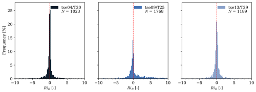
Figure 9 Histogram of the bulk Richardson number from 10 min average measurements at tse04/T20 (SW ridge), tse09/T25 (valley), and tse13/T29 (NE ridge) at 100 m a.g.l. during the VM measurement periods of the mean flow. The Ri_B values are constrained to the −10 to 10 interval, with a bin width of 0.2.

From the data collected by the 100 m towers, the following number of 10 min periods were classified as unstable (stable) at VM1–3: 526 (497), 780 (988), and 617 (572) for the mean wind components at 100 m a.g.l. For the variances, the respective quantities were 447 (383) at VM1, 719 (898) at VM2, and 552 (514) at VM3.

The influence of atmospheric stability on the dual-lidar results was affected by the distinct wind flows between the ridges and the valley in Perdigão (Table 8), as well as by the different spatial (WSs' interception angle) and temporal (WSs' desynchronisation) configurations among the VMs. On the ridges, VM1 and VM3 showed slightly better r² values and slightly lower errors under stable compared to unstable atmospheric conditions, especially for turbulent flow variables. The average r², RMSE, and bias for the mean wind components (u and v) were 0.997, 0.414 m s⁻¹, and 0.082 m s⁻¹ in stable conditions, while under unstable conditions, these were equal to 0.996, 0.434 m s⁻¹, and 0.075 m s⁻¹. For turbulence variables ($u^{\prime }{u}^{\prime }$ and $v^{\prime }{v}^{\prime }$), the statistical metrics assumed mean values of 0.853, 0.235 m² s⁻², and −0.055 m² s⁻² for stable, and 0.836, 0.339 m² s⁻², and −0.140 m² s⁻² for unstable conditions.

Table 8 Statistical parameters from VM and tower comparisons according to the atmospheric stability.

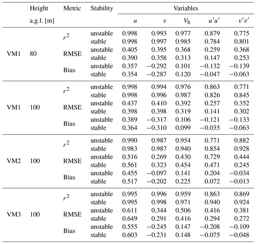
The RMSE and bias units are m s⁻¹ for u, v, and V_h variables, while for $u^{\prime }{u}^{\prime }$ and $v^{\prime }{v}^{\prime }$ the units are m² s⁻². r² is unitless.

Conversely, at the valley VM, higher r² values and lower errors with a stable atmosphere were restricted to $u^{\prime }{u}^{\prime }$ and $v^{\prime }{v}^{\prime }$. The variances r², RMSE, and bias under stable conditions were 0.891, 0.358 m² s⁻², and 0.029 m² s⁻², on average. In comparison, the average $u^{\prime }{u}^{\prime }$ and $v^{\prime }{v}^{\prime }$ metrics during unstable conditions were equal to 0.827, 0.587 m² s⁻², and 0.085 m² s⁻². Another distinct result at VM2 was that regardless of the atmospheric conditions; the $u^{\prime }{u}^{\prime }$ turbulence measurement overestimated the tse09/T25 sonic anemometer readings at 100 m a.g.l.

The overall better results from the VMs under stable compared to unstable atmospheric conditions indicate that when the air is more stable and less turbulent, the temporal and spatial synchronisation between the scans of a multi-lidar system becomes less critical, without compromising the accuracy of the measurements. Additionally, while the statistical metrics for the 10 min mean values changed slightly according to stability, the metrics for the 10 min variances were more affected by atmospheric conditions. In terms of wind direction, there was no clear relationship between the VM wind direction error (i.e. the difference between the VM's 10 min average horizontal wind direction and the tower's 10 min average horizontal wind direction) and atmospheric stability (not shown here).

4.2.2 Vertical velocity

Another possible influence on VM retrievals was the assumption of a zero vertical wind velocity (w) made to obtain the horizontal wind components from the WindScanners' radial velocities (Step 4 in Sect. 3.1). The coefficient of determination of the linear regression between the 10 min average w values measured by sonic anemometers and the 10 min horizontal wind speed errors of the VMs (i.e. the difference between the VM's 10 min average horizontal wind speed and the anemometer's 10 min average horizontal wind speed) around 100 m a.g.l. in Perdigão was lower than 0.060 at all measurement locations. For turbulence measurements, the highest r² between the 10 min average w values and the 10 min VM measurement errors was 0.110 at VM1.

These low r² values mean that the assumption of zero vertical wind velocity had a minimal impact on the VM measurements at 80 and 100 m a.g.l. in Perdigão, confirming the validity of the VM results at these heights. This minimal impact is attributed to the small elevation angles of the lidars' beams (Table 2) and the low vertical velocity at the site, which did not exceed 3.6 m s⁻¹ at 100 m a.g.l. during the IOP.

At heights above 100 m, however, the elevation angles of the beams will be higher, causing the lidar beams to be more aligned with the vertical component of the wind. Thus, in a strong convective atmosphere at higher heights, the vertical velocity can influence the virtual-mast results more significantly. In Perdigão, the maximum elevation angles of the VMs were 21.6° at VM1, 15.6° at VM2, and 23.0° at VM3.

4.2.3 Sampling rate

We turned to the sonic data to assess how the VM sampling rate affected the results. Results at progressively lower sampling rates were compared against the 20 Hz measurements in terms of r², RMSE (Fig. 10), and bias. The data were downsampled by selecting every nth sample for frequencies between 1 and 20 Hz (e.g. for 2 Hz, every 10th sample) and by selecting the nth time step for frequencies below 1 Hz (e.g. for 0.5 Hz, every second time step). Following downsampling, variances and averages were calculated over 10 min intervals. Then, to assess the influence of the sampling rate in the VM retrievals, the statistical metrics of the sonic data were linearly interpolated at the VMs' acquisition rates, between 0.018–0.038 Hz for the means and 0.030–0.038 Hz for the variances (shaded area in Fig. 10).

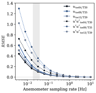
Figure 10 RMSE of sonic measurements by the sampling rate, for the mean (u) and turbulent ($u^{\prime }{u}^{\prime }$) x-axis wind speed component, on the three 100 m towers at 100 m a.g.l. The RMSE units are m s⁻¹ for u and m² s⁻² for $u^{\prime }{u}^{\prime }$.

Similar to the previous results, the mean wind flow (u, v, and V_h) and the metrics r² and bias showed less sensitivity to measurement frequency than the variances ($u^{\prime }{u}^{\prime }$ and $v^{\prime }{v}^{\prime }$) and RMSE at the three 100 m towers. Additionally, the sampling rate had a similar influence on the wind components of the same moment, evidenced by the comparable results for u and v and for $u^{\prime }{u}^{\prime }$ and $v^{\prime }{v}^{\prime }$ at Table 9. Consequently, Fig. 10 displays only the RMSE for mean and turbulent x-axis wind speed component at 100 m a.g.l.

Table 9 Averaged statistical metrics due to sampling rates in the virtual-mast measurement range for the mean (0.018–0.038 Hz) and turbulent (0.030–0.038 Hz) flow, based on sonic readings at 100 m a.g.l.

The units of RMSE and bias are m s⁻¹ for mean variables, while for variances they are m² s⁻². r² is unitless.

At 100 m a.g.l., the estimated average RMSE of the VMs, due solely to their sampling rate, ranged between 0.102 and 0.180 m s⁻¹ for the mean flow quantities and 0.262 and 0.306 m² s⁻² for the turbulence variables (Table 9). Considering the overall RMSE values for all virtual masts at 100 m a.g.l. (0.434 m s⁻¹ for the average of u and v and 0.363 m² s⁻² for the average of $u^{\prime }{u}^{\prime }$ and $v^{\prime }{v}^{\prime }$), around 33 % of the VMs' RMSE for the mean wind components and 78 % for the variances can be attributed to their measurement frequency, assuming a linear influence of this factor. For the mean horizontal wind velocity, 33 % of the VMs' average RMSE at 100 m a.g.l. can be attributed to their measurement frequency. Additionally, to accurately measure the wind flow in the valley, a higher sampling rate is required than above the hills, especially to retrieve the wind variances. Within the VM sampling rate range, the average RMSE error for turbulence measurements at 100 m a.g.l. is about 61 % and 19 % higher in the valley than on the SW and NE ridge.

Therefore, when aiming for dual-lidar readings with errors due to the sampling rate lower than those presented here, one should evaluate the elevation range covered in the RHI mode, the lidar's acquisition time, and the type of scan. Additionally, the influence of the sampling rate on measurements should be considered when planning new experimental campaigns, particularly in the selection of equipment and measurement frequency of targeted wind variables. For a minimum RMSE increase (below 0.1 m s⁻¹ and 0.1 m² s⁻²) compared to the 20 Hz frequency, the VM sampling rate should be at least 0.05 Hz for mean quantities and 0.2 Hz for turbulence measurements.

5 Conclusions

Dual-lidar measurements of range height indicator (RHI) scans in a virtual-mast (VM) mode were compared against sonic anemometer readings at three 100 m towers over the Perdigão complex terrain to evaluate the VM measurement uncertainty and validate its use over large distances above the ground. The study focused on 10 min means and variances of radial velocity (v_r), wind speed (V_h), and wind velocity (u and v), retrieved by dual-lidar and sonic anemometers at 80 and 100 m a.g.l. A methodology for processing the virtual-mast dataset was also devised.

In the analysis of the mean flow, a high correlation was found between VM and sonic measurements, with r² values close to 1 at all VMs. Notably, the lowest r² were observed at VM2 (0.987 for u and v, and 0.948 for V_h), attributed to the small angle (∼ 40.2°) between the lidars' beams (leading to high dual-lidar error propagation) and to the more turbulent flow in the valley. Regarding the errors, the average RMSE and bias for u and v was 0.422 m s⁻¹ and 0.102 m s⁻¹ for all VMs, with the highest values occurring at VM3, 0.626 m s⁻¹ and 0.575 m s⁻¹, for the u component. The error magnitudes were consistent for all mean flow variables (u, v, and V_h) within each virtual mast. However, the average r² for V_h (0.969) was lower than that for the wind components (0.994).

The low measuring frequency (0.038 Hz maximum) and the VM location mainly impacted the turbulence measurements ($u^{\prime }{u}^{\prime }$ and $v^{\prime }{v}^{\prime }$). The average r² that was equal to 0.994 for the mean wind components was 0.867 for the variances. In the linear regression equation, the constants (b) took on values close to zero for all VMs, while the slope coefficients (m) varied from 0.799 for $v^{\prime }{v}^{\prime }$ VM1 to 1.269 for $u^{\prime }{u}^{\prime }$ VM2. The greater sensitivity of VM2 to turbulence changes, however, did not translate into better accuracy. The RMSE for $u^{\prime }{u}^{\prime }$ and $v^{\prime }{v}^{\prime }$ across all VMs averaged 0.340 m² s⁻², with the highest value observed in the valley (VM2), reaching 0.600 m² s⁻² for $u^{\prime }{u}^{\prime }$, due to the worse lidars' synchronisation (about 9 s), the smaller between-beam angle, and the complex valley flow. Overall, the VM correlations against reference turbulence measurements were still high, and the average errors were low (0.340 m² s⁻² RMSE and −0.063 m² s⁻² bias), indicating that small-scale phenomena play a smaller role at 80 and 100 m a.g.l. in Perdigão.

The influence of atmospheric stability also depended on the VM location. The virtual masts on the ridges (VM1 and VM3) showed higher correlations and lower errors under stable compared to unstable conditions. Namely for the variances, where the average r², RMSE, and bias for VM1 and VM3 under stable (unstable) conditions were equal to 0.853 (0.836), 0.235 m² s⁻² (0.339 m² s⁻²), and −0.055 m² s⁻² (−0.140 m² s⁻²). In the valley (VM2), the better statistical metrics with stable conditions were restricted to the variance measurements of the wind, showing average r², RMSE, and bias of 0.891 (0.827), 0.358 m² s⁻² (0.587 m² s⁻²), and 0.029 m² s⁻² (0.085 m² s⁻²) with stable (unstable) atmosphere. Although atmospheric stability differently affected the accuracy of VM measurements on the ridges and in the valley, the results indicate that in a stable, less turbulent atmosphere, synchronisation between the scans of a multi-lidar system becomes less critical for maintaining measurement accuracy than in unstable conditions. Regarding the VM wind direction, no correlation between its errors and atmospheric stability could be drawn.

The impact of the zero vertical velocity assumption on dual-lidar retrievals at 80 and 100 m a.g.l. in Perdigão was minimal, confirming the validity of the VM results at these heights. The r² results were lower than 0.060 for the 10 min average w values from sonic anemometer readings and the 10 min horizontal wind speed errors from the VM measurements, and they were lower than 0.110 for the 10 min average w values and the 10 min variance errors from the VMs.

Lastly, the influence of the VM sampling rate accounted for 33 % of the overall RMSE for the mean quantities and 78 % for the variances at 100 m a.g.l. when assuming a linear influence of this factor on the dual-lidar error. The impact of sampling rate on measurements, including those from dual lidars, is crucial when selecting and configuring equipment to ensure accurate recording of target variables.

Overall, Perdigão's VMs obtained accurate mean flow measurements, and their turbulence estimations, despite displaying lower correlations against reference data, also showed low errors, demonstrating the VMs' ability to capture mean and turbulent wind characteristics under different flow conditions, at great heights, and in complex terrain. From the VM measurements and sonic readings, the construction of vertical profiles of the wind enables the analysis of Perdigão's complex flow at heights up to 430 m a.g.l.

For greater data accuracy and reliability in future dual-lidar campaigns, the lidars must be positioned to form an approximately 90° angle between their beams to minimise error propagation and operated at a sampling frequency of at least 0.05 Hz for mean quantities and 0.2 Hz for turbulence. These frequencies yield a minimal RMSE increase (below 0.1 m s⁻¹ and 0.1 m² s⁻²) compared to the 20 Hz frequency.