Putting the spotlight on small cloud droplets with SmHOLIMO – a new holographic imager for in situ measurements of clouds

The microstructure of liquid and mixed-phase clouds is characterized by the cloud droplet size distribution (CDSD), which influences the cloud evolution and its interaction with radiation. However, state-of-the-art cloud probes still face challenges because they require either platforms that move at constant speed or inlets that can directly alter the actual CDSD. Therefore, precise and accurate in situ measurements of CDSDs, especially of cloud droplets smaller than 6 µm, are still lacking. This can lead to uncertainties in the microphysics and thus in weather and climate models, which are based on parameterizations often derived from these measurements.

We present a new in situ instrument, the Small Holographic Imager for Microscopic Objects (SmHOLIMO), specifically designed to measure a broad spectrum of the CDSDs, i.e., from 3.7 to ≈100 µm, with a sample volume rate of 2.5 cm³ s⁻¹. Thereby, SmHOLIMO pushes the resolution limit towards the limits seen with forward-scattering probes, while still maintaining the advantages of open-path holography, i.e., a well-defined sample volume (operation at variable wind speed); no need for an inlet; independence of particle size, phase, refractive index, and shape; and the potential of spatial analyses. After calibrating SmHOLIMO in the laboratory, the instrument was deployed in the field, on a tethered balloon system, probing a dissipating low stratus. We demonstrate its ability to measure the cloud microphysical properties at high spatio-temporal resolution. Furthermore, we compare the SmHOLIMO observations to those of another holographic imager (resolution: 6 µm) and to co-located remote sensing measurements. We unequivocally show the importance of SmHOLIMO's skills to capture the lower tail of the CDSD, which significantly affects the derived quantities of cloud droplet mean diameter (up to 1.6 times smaller), number concentration (up to 4 times higher), and cloud optical depth (up to 2.7 times higher). SmHOLIMO's high-resolution in situ data of cloud droplets will help us to better interpret observations and to refine the representation of clouds in climate and weather models.

1 Introduction

In situ measurements of the microphysical properties and the large-scale cloud structure remain a cornerstone of our understanding of Earth's climate. The diverse and complex processes controlling clouds range from the microscale, where cloud hydrometeors interact with each other to form precipitation, to the synoptic scale, where they interact with solar and terrestrial radiation and mediate the radiative budget of our planet. An important quantity used to characterize clouds is the cloud droplet size distribution (CDSD) (Allwayin et al., 2024), as it provides information on the processes involved in cloud formation, temporal evolution, and persistency; the efficiency of the collision–coalescence process to form precipitation; radiative properties; and much more. Since in situ measurements of clouds and particular their evolution are only available sparsely, we rely heavily on weather and climate models to achieve full coverage in predicting a cloud's evolution and impacts. In these models, cloud microphysical processes and their interactions often have to be represented in the form of parameterizations, which can introduce large uncertainties (Morrison et al., 2020). Such parameterizations in turn are often based on in situ measurements (e.g., Khairoutdinov and Kogan, 2000; Lohmann and Diehl, 2006; Ickes et al., 2015), which highlights the importance of improving the accuracy and precision of in situ observations through continued advancements in cloud measurement techniques.

A promising in situ measurement approach is in-line holography, which has been applied for cloud measurements for more than 40 years (e.g., Conway et al., 1982; Kozikowska et al., 1984; Borrmann and Jaenicke, 1993). Since the introduction of digital in-line holography in the mid-90s (Lawson and Cormack, 1995), the setup of holographic instruments has become relatively simple and robust, yielding widespread use in stationary ground-based field measurements (e.g., Raupach et al., 2006; Henneberger et al., 2013; Kaikkonen et al., 2020) and on a multitude of moving platforms like aircraft (e.g., Fugal and Shaw, 2009; Beals et al., 2015; Schlenczek, 2018; Glienke et al., 2020; Allwayin et al., 2024), gondolas (Beck et al., 2017), launched balloons (Chambers et al., 2024), and tethered balloon systems (TBSs) (e.g., Ramelli et al., 2020; Stevens et al., 2021).

As for any measurement technique, in-line holography comes with its own unique advantages and disadvantages, which are summarized in Baumgardner et al. (2011). Advantages are that assumptions on the cloud particle shape, orientation, and phase are not needed because real images are captured. Secondly, holography provides information on the three-dimensional location of cloud particles within the sample volume, which allows the study of fine-scale cloud droplet clustering and non-uniformity down to centimeter scales (Beals et al., 2015; Larsen et al., 2018; Glienke et al., 2020). Thirdly, in-line holography has a well-defined sample volume that is independent of the cloud particle sizes, and it can be implemented in an open-path setup (no inlet and suction pump required), facilitating measurements under variable wind speeds and not being reliant on moving platforms, such as aircraft (Baumgardner et al., 2011). Finally, it can measure cloud particles over a wide size range (6 µm–1 cm) with high spatio-temporal resolution.

One disadvantage of in-line holography is that the sample volume V_hol strongly depends on the desired resolution D_res ($V_{\text{hol}}\propto D_{\text{res}}^{\mathrm{4}}$, derivation see Henneberger, 2013). This limits the maximum resolution usually to values around 6 to 10 µm (see Fugal and Shaw, 2009; Ramelli et al., 2020; Baumgardner et al., 2011). Forward-scattering cloud probing instruments reach resolutions of 2 µm, such as the Cloud Droplet Probe (CDP-2; Droplet Measurement Techniques, USA) or the Fog Monitor (FM-120; Droplet Measurement Techniques, USA), which however need assumptions on particle shape, orientation, and refractive index. The main reason that the resolution of holographic imagers is limited to around 6 to 10 µm is that they are designed to reliably observe both liquid and ice phase particles. Since under natural conditions ice crystal concentrations are usually several orders of magnitudes lower than cloud droplet concentrations (a few per liter vs. a few hundred per cubic centimeter), a compromise between sample volume and resolution is needed, which means consciously losing the ability to observe small cloud droplets. A second disadvantage is the large number of data produced for holographic measurements, which easily reaches the order of TB. The evaluation of these data includes a computational expensive reconstruction step and a time-consuming and complex data analysis. Due to technical advancements, the storage of a large number of data does not pose a challenge anymore, but the numerical reconstruction remains a bottleneck in holography.

In this study, we present the Small Holographic Imager for Microscopic Objects (SmHOLIMO), a newly developed instrument specifically designed to measure cloud droplets down to small scales (3.7 µm) in conditions of low and variable wind speeds (<10 m s⁻¹), such as seen for ground-based or balloon-borne applications. SmHOLIMO thereby retains the advantages of holography (open-path configuration, well-defined sample volume, and potential for spatial analysis) while nearing the resolution of forward-scattering probes. During development, we approached the technical and hardware limitations of commercial off-the-shelf components needed to achieve the high resolution, while maintaining a large enough sample volume for sufficient counting statistic for large droplets.

We will start by introducing the measurement principle of SmHOLIMO, the setup in Sect. 2, and the laboratory characterization and calibration in Sect. 3. In Sect. 4 we present a case study in which SmHOLIMO probes a dissipating low stratus cloud. We compare the SmHOLIMO observations with those of a co-located measurement using another holographic imager (HOLIMO). We thereby demonstrate the importance of SmHOLIMO's ability to measure a broader spectrum of CDSD, which is needed to fully characterize clouds and their radiative properties, especially in the cloud base region where cloud droplet formation takes place. Finally, we compare the SmHOLIMO and HOLIMO observations with remote sensing measurements from a microwave radiometer and a cloud radar.

2 The Small Holographic Imager for Microscopic Objects: SmHOLIMO

The Small Holographic Imager for Microscopic Objects (SmHOLIMO) is the fifth-generation and latest holographic imager developed in the Atmospheric Physics group at ETH, Zurich. The setup is based on the expertise gained from previously developed holographic instruments such as that shown in Amsler et al. (2009), Henneberger et al. (2013), Beck et al. (2017), and Ramelli et al. (2020). In contrast to previous instruments, SmHOLIMO is specifically designed to obtain accurate in situ measurements of cloud droplets in the size range from 3.7 to ≈100 µm. Since the sample volume scales with the spatial resolution as $V_{\text{hol}}\propto D_{\text{res}}^{\mathrm{4}}$, the sample volume of SmHOLIMO is ≈0.5 cm³ and thus significantly smaller than the volumes of other holographic imagers, typically ranging from 15 to 20 cm³ (e.g., Spuler and Fugal, 2011; Ramelli et al., 2020). This does not exclude the possibility to detect ice crystals, but due to the small sample volume rate of SmHOLIMO of max ≈5 cm³ s⁻¹ and the generally low occurrence of ice crystals on the order of <10 L⁻¹, obtaining robust results for the ice phase will be challenging. Therefore, in this study we will focus on the liquid phase only.

2.1 Working principle of digital in-line holography

The working principle of SmHOLIMO is based on digital in-line holography. Holography can generally be divided into two main parts: (1) the generation of holograms and (2) the numerical retrieval of single-particle information from the holograms.

To generate and record a hologram, a coherent light source (i.e., laser) and a digital camera are required. The beam of the coherent light source is first collimated (reference wave) before traversing the sample volume. If particles are present in the sample volume, they will cause diffraction, resulting in a secondary wave (diffracted wave) that interferes with the reference wave (see Fig. 1a). A digital camera records this wavefront as a two-dimensional hologram. A more complete and comprehensive description of holography can be found in Kreis (2005) and Picart and Li (2012).

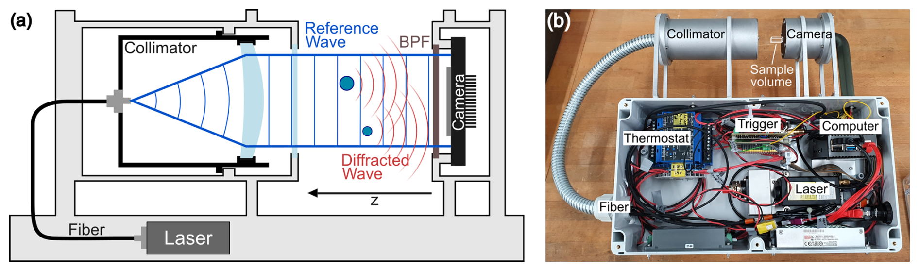
Figure 1 (a) Sketch of the working principle of SmHOLIMO and digital in-line holography. A laser beam is collimated (reference wave) before traversing the sample volume. Particles in the sample volume cause diffraction, resulting in a secondary wave (diffracted wave) that interferes with the reference wave. A camera records the resulting wavefront as a two-dimensional hologram. A band-pass filter (BPF) is mounted in front of the camera to reduce stray light. (b) Annotated image of SmHOLIMO showing the main components.

The three-dimensional location, shape, and size of the observed particles are numerically reconstructed from the hologram using the HoloSuite software package described in Fugal et al. (2009). The location is determined by the center voxel where the particle is in focus and the shape is a direct result of the given particle shadowgraph at this position. The particle size is inferred from the camera pixel sizes using a sizing algorithm described in Sect. 3.2. Only particles with a diameter larger than 3.7 µm (i.e., 2 px × 2 px) are analyzed (see Sect. 3.1) to reduce the detection of artifacts due to camera sensor noise. The particles are classified into cloud droplets and artifacts based on their shape by a neural network (Touloupas et al., 2020). For more accurate classification, the neural network is fine-tuned using a subset of 512 hand-labeled particles and artifacts for each recorded data set.

2.2 Hardware design

SmHOLIMO's primary deployment sites are either ground-based locations (e.g., mountain tops) or balloon-borne platforms (e.g., TBS; see Sect. 4), which typically experience highly variable wind conditions. Therefore, SmHOLIMO was specifically designed to be lightweight (≈5.3 kg) and compact, measuring $\mathrm{45}\mathrm{cm}\times \mathrm{40}\mathrm{cm}\times \mathrm{13}\mathrm{cm}$ (height × width × depth). Due to the open-path configuration of SmHOLIMO, the effects of non-isokinetic sampling of cloud droplets are minimized, and the well-defined sample volume facilitates measurements with low and variable inflow velocities, which allows it to be used as a ground-based instrument (e.g., mountain tops). An image of the final instrument including its main components is shown in Fig. 1b.

A 409 nm¹, 150 mW laser diode (Cobolt 06-MLD 405 nm, Hübner Photonics GmbH, Germany) is used as coherent light source and is operated in digital modulation mode. The laser diode is modulated by homemade electronics that generates stable 220 ns laser pulses to reduce motion blur of moving cloud droplets. The laser beam is guided via an optical fiber and collimating optics (fiber coupler: 60SMF-1-4-M5-33, fiber: SMC-E-400Si-3.3-NA012-3-APC.EC-0-100, collimator: 60FC-T-4-M75-01, Schäfter+Kirchhoff GmbH, Germany) that expands the beam to a diameter of 10.5 mm ($\mathrm{1}/{\mathrm{e}}^{\mathrm{2}}$ width), before traversing the open-path sample volume. A sapphire window seals the collimator from the sample volume. A bare-board machine vision camera (AV ALVIUM 1800U-1240M-BB, Stemmer Imaging, Germany) with 4024 px × 3036 px, 12.5 Mp, and 1.85 µm × 1.85 µm pixel pitch (camera sensor: Sony IMX226) captures holograms with a maximum acquisition frame rate of 30 fps. However, the data transfer speed of the single-board computer limits the frame rate in field operations to 10 fps. A band-pass filter (FBH410-10, Thorlabs, USA) with a central wavelength of 410 nm and bandwidth of 10 nm in front of the camera seals the camera housing and reduces atmospheric stray light. In addition, for very bright conditions, two black stray-light plates can be mounted on either side of the sample volume. The two housings for the collimator and camera are made of 3D printed aluminum and are mounted at a distance of 20 cm from the electronics box to reduce aerodynamic effects of the housing on the sample volume. To withstand icing conditions, i.e., measurements in supercooled clouds, the aluminum housings are equipped with thermocouples and two 50 W heating cartridges that are controlled by a thermostat (TR250, Ziehl, Germany).

A single-board computer (Raspberry Pi 4 Model B – 8 GB) synchronizes the triggering of the laser pulses with the acquisition of holograms and stores the recorded holograms on an external SSD hard drive. The computer also allows direct access via a VNC connection during measurement periods and yields live data of the measurements with information regarding their quality.

3 Instrument characterization and validation of the sizing algorithm

To ensure that SmHOLIMO can retrieve accurate cloud microphysical properties such as CDSDs, the optical resolution of the instrument over the sample volume must be determined (Sect. 3.1), and the particle sizing algorithm must be validated (Sect. 3.2).

3.1 Optical resolution measurements

A uniform optical resolution across the whole sample volume is important to avoid a sampling bias linked to the size of cloud droplets. For SmHOLIMO, the optical resolution is limited by (1) the diffraction-limited resolution imposed by the working principle of digital in-line holography and (2) the pixel resolution limit of the camera pixel pitch.

The diffraction limited resolution

$$D_{\text{res,rec}}\left(z_{\text{rec}}\right)={\displaystyle \frac{\mathrm{2.44}\cdot \mathit{\lambda }}{D_{\text{cam,eff}}}}\cdot z_{\text{rec}}$$

is derived from half the Rayleigh criterion and is a linear function of the reconstruction depth z_rec (orthogonal distance from the camera sensor along the z direction; see Fig. 1a) and the laser wavelength λ. The effective camera sensor aperture is given by $D_{\text{cam,eff}}=\sqrt{D_{\text{cam},x}\cdot D_{\text{cam},y}}$ with the camera sensor dimensions $D_{\text{cam},x}=\mathrm{7.44}\mathrm{mm}$ and $D_{\text{cam},y}=\mathrm{5.62}\mathrm{mm}$ along the two sensor dimensions. The diffraction limited resolution D_res,rec(z_rec) for SmHOLIMO is shown in Fig. 2 as a solid black line.

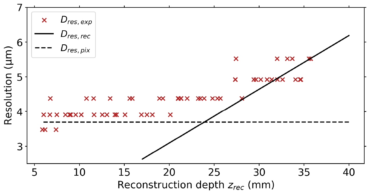
Figure 2 Optical resolution measurements and theoretical limits over the reconstruction depth z_rec for SmHOLIMO. The measured resolutions D_res,exp (red crosses) are determined using a 1951 USAF resolution test chart. The solid black line shows the diffraction resolution limit D_res,rec(z_rec), and the dashed black line indicates the pixel resolution limit D_res,pix.

The pixel resolution limit D_res,pix for SmHOLIMO is given by

$$D_{\text{res,pix}}=\mathrm{2}\cdot d_{\text{pix}}=\mathrm{3.7}\mathrm{\mu }\mathrm{m},$$

with d_pix=1.85 µm the equilateral pixel size for our camera sensor. It is shown in Fig. 2 as a dashed black line. A more general and detailed derivation of both resolution limits can be found in Henneberger (2013).

The optical resolution D_res,exp of SmHOLIMO was verified by placing a 1951 USAF resolution test chart in different reconstruction depths $\mathrm{6}<z_{\text{rec}}<\mathrm{35}$ mm within the sample volume, as was done by Spuler and Fugal (2011), Beck (2017), and Ramelli et al. (2020). The resolution was determined manually by identifying the smallest recognizable pattern (three bars) on the resolution chart, and the results are shown in Fig. 2 as red crosses. All measured resolutions are close to the theoretical limits and follow the expected increase for z_rec>24 mm imposed by D_res,rec(z_rec). Although the increase in resolution limit beyond z_rec=25 mm is known and could be corrected for, we restrict the SmHOLIMO reconstruction depth to this value. This ensures the highest and a uniform optical resolution across the entire sample volume while maintaining a sample volume that is independent of cloud droplet size.

3.2 Validation of the particle sizing algorithm

To ensure that SmHOLIMO accurately measures cloud droplet diameters, we want to validate the particle sizing algorithm. The sizing algorithm is embedded within the HoloSuite software package and was introduced by Beck (2017). It is based on a brightness threshold between the observed droplet shadowgraph (dark) and the background (bright) within a hologram, which allows the particle sizing algorithm to be tuned.

The validation of the sizing algorithm is performed using a vibrating orifice aerosol generator (VOAG; model 3450, TSI, USA) that produces a jet of droplets from an isopropanol-polyethylene glycol emulsion. After the VOAG, the droplet jet was dispersed into a homogeneous plume by passing it through a ventilated cylinder (12 cm×1 m, flow rate of 50–70 L min⁻¹). The residence time within the cylinder was ≈11 s to ensure full evaporation of the isopropanol yielding nearly monodisperse droplets of polyethylene glycol. A total of six different droplet sizes were generated, with diameters ranging from ≈4 to ≈19 µm (see Table 1). The six different validation experiments were conducted in a co-located measurement setup, using SmHOLIMO and an aerodynamic aerosol sampler (APS, model 3321, TSI, USA) serving as the ground truth instrument. The APS can measure droplets in the size range between 0.5 and 20 µm.

To validate the sizing algorithm of SmHOLIMO, the brightness threshold was varied between 0.40 and 0.75. The best agreement (minimum sum of squared errors) between the SmHOLIMO and APS measurements was found for a brightness threshold of 0.45. However, we decided to exclude the measurements with droplet diameters of 19 µm because this size is close to the upper observable limit of the APS. This likely leads to an underestimation of the droplet sizes due to a sampling bias toward smaller droplets. The best agreement was found with a threshold of 0.5 after removing the measurements at 19 µm.

Table 1 Measured diameters of the size algorithm validation of SmHOLIMO for six different droplet sizes and a brightness threshold of 0.5. For the aerodynamic particle sizer (APS), means and standard deviations are retrieved from Gaussian functions that are fitted to the normalized size distributions (see Fig. 3). For SmHOLIMO, means and standard deviations are retrieved directly from the distribution of the single-particle data.

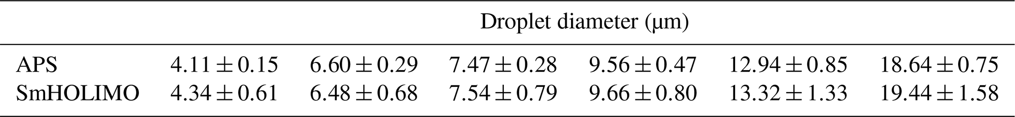
The measured APS and SmHOLIMO droplet size distributions for a brightness threshold of 0.5 are shown in Fig. 3 and are normalized to their maxima. We see a general trend of SmHOLIMO slightly overestimating the droplet diameters compared to the APS except for the 6 µm measurements. The highest relative deviations are found for the 4 µm droplets with 6 % and the 19 µm droplets with 4 %, since these sizes are situated at the observable limits of SmHOLIMO and the APS, respectively. As mentioned previously, for the 19 µm experiment, we assume a sampling bias towards smaller droplet sizes from the APS. Conversely, for the 4 µm droplets, SmHOLIMO is assumed to overestimate the droplet size, as the diameter is just above the resolution limit of 3.7 µm. Overall, the droplet diameters measured by SmHOLIMO and APS are in good agreement without any significant deviations, and all measurements fully overlap within their respective uncertainties (see Table 1 and Fig. 3).

Spatially resolved information on the homogeneity of the recorded droplets and the performance of the sizing algorithm is shown in the Appendix (Fig. A1) for each droplet size individually. We observe a uniform droplet count distribution after trimming the sample volume to remove hologram edge effects. Furthermore, no dependence between droplet size and sample volume location can be inferred.

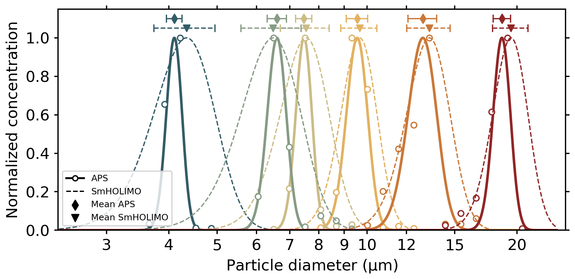
Figure 3 Normalized APS and SmHOLIMO size distributions with a brightness threshold of 0.5 for six size algorithm validation experiments with different droplet diameters (colors) ranging from ≈4 to ≈19 µm. The APS means (diamond) and standard deviations (solid bars) are retrieved from Gaussian functions (solid lines) that are fitted to the APS measurements (circles). The SmHOLIMO means (triangles) and standard deviations (dotted bars) are retrieved directly from the distribution of the single-particle data, and the Gaussian functions (dashed lines) are derived from them.

4 Case study: measuring a low stratus cloud

The performance of SmHOLIMO was also evaluated in the field, where SmHOLIMO was deployed on a tethered balloon system. During a case study on 29 February 2024, SmHOLIMO observed a dissipating low stratus cloud over the Swiss Plateau. Here we present the observations of 30 profiles taken between 08:09 and 10:21 UTC through the entire cloud layer (see Table B1, Fig. 4). This study provides an ideal test case to investigate the performance of SmHOLIMO due to the generally small cloud droplets in wintertime stratus (Lohmann et al., 2016; Ramelli et al., 2020) and the availability of cloud measurements from the cloud base to cloud top. These measurements were performed within the CLOUDLAB project, where an extensive set of in situ and ground-based remote sensing instrumentation was deployed (see Henneberger et al., 2023).

We will first describe the measurement setup and data analysis (Sect. 4.1), and the meteorological conditions (Sect. 4.2), before comparing the in situ observations of SmHOLIMO to co-located HOLIMO (HOLIMO; see Ramelli et al., 2020, 2021) observations (Sect. 4.3) and remote sensing measurements (i.e., microwave radiometer and cloud radar, Sect. 4.4).

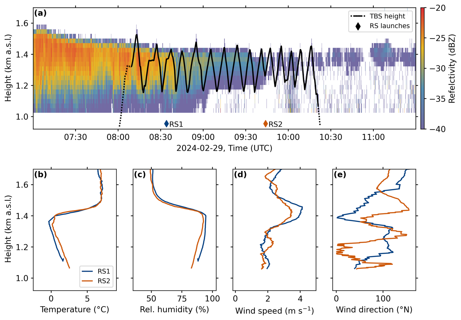
Figure 4 Meteorological conditions during the cloud measurements on 29 February 2024. (a) Height–time indicator (HTI) reflectivity measurements (in dBZ) of a vertically pointing W-band Doppler cloud radar of a dissipating low stratus between 07:00 and 11:30 UTC. The time and height of the 30 vertical profiles (dotted and solid black line) of the tethered balloon system (TBS) are shown. The dotted black sections indicate times when no in situ measurements were taken. The launch times of two radiosondes (RS1, 08:34 UTC, blue diamond; RS2, 09:46 UTC, orange diamond) are shown at the bottom. The meteorological variables of RS1 (blue) and RS2 (orange) are shown as vertical profiles in (b) temperature, (c) relative humidity, (d) wind speed, and (e) wind direction.

4.1 The measurement setup and data analysis

The measurement location is close to Eriswil (47°04^′14^′′ N, 7°52^′22^′′ E) at an altitude of 920 m a.s.l. For the in situ observations, we used a tethered balloon system (TBS, HoloBalloon, Ramelli et al., 2020; Henneberger et al., 2023), which can lift an instrumentation platform of around 80 kg inside the low stratus cloud. The platform carried SmHOLIMO and HOLIMO, mounted with a horizontal displacement of around 1.5 m, hanging 30 m below the TBS. The height of the TBS was adjusted using a winch, with a vertical velocity of 1.5 m s⁻¹ during ascent and of 1 m s⁻¹ during descent, which results in an average profile duration of 5 min.

The SmHOLIMO data were recorded and analyzed with a frequency of 5 Hz, and the reconstruction volume was trimmed to $-\mathrm{3.2}<X<\mathrm{3.2}$, $-\mathrm{2.2}<Y<\mathrm{2.2}$, and $\mathrm{7}<Z<\mathrm{25}$ mm, yielding a sample volume of V_hol=0.5 cm³ and a sample volume rate of 2.5 cm³ s⁻¹. The primary objective of the measurements is to observe the large-scale temporal evolution of the cloud. Therefore, a recording frequency of 5 Hz was chosen instead of the maximum 10 Hz to enable continuous measurements for 4.6 h, constrained by the 1 TB storage capacity. Additionally, we average the SmHOLIMO data over 1 s, as our focus (in this specific measurement) is not on capturing small-scale fluctuations in cloud microphysical properties. This also ensures consistency in time resolution with HOLIMO while further improving the measurement accuracy through enhanced counting statistics.

The HOLIMO data were analyzed with a frequency of 1 Hz, and the reconstruction volume was trimmed to $-\mathrm{6.5}<X<\mathrm{6.8}$, $-\mathrm{7.0}<Y<\mathrm{6.5}$, and $\mathrm{40}<Z<\mathrm{120}$ mm, resulting in an sample volume rate of 14 cm³ s⁻¹. The average vertical resolution for both instruments was 1.25 m.

The detected particles were classified into cloud droplets and reconstruction artifacts using a neural network (Touloupas et al., 2020) that has been fine-tuned using the respective data set (see Sect. 2.1). Cloud droplets with diameters >20 µm for SmHOLIMO and >30 µm for HOLIMO were manually classified into the same categories. The derivation of cloud microphysical variables, i.e., liquid water content (LWC), cloud droplet number concentration (CDNC), and cloud optical depth τ_c, was constrained to LWC >0.01 g m⁻³ (“in cloud” definition). The derivation of the cloud droplet mean diameter is further constrained to CDNC >20 cm⁻³ for statistical reasons. The uncertainty in retrieving the diameter of a single droplet with SmHOLIMO is defined by the pixel pitch, yielding Δd_s=1.85 µm (Fugal et al., 2004; Adrian and Westerweel, 2011). When measuring N independent droplets, the total uncertainty decreases according to the central limit theorem due to random error reduction, resulting in $\mathrm{\Delta }{d}_N=\mathrm{\Delta }{d}_{\mathrm{s}}\cdot {\sqrt{N}}^{-\mathrm{1}}$. The uncertainty associated with CDNC follows counting statistics and is thus described by $\sqrt{N}$, where N represents the total number of detected droplets. Exemplary CDSDs, including their corresponding uncertainties, are presented in Fig. C1. Additionally, reconstruction quality in in-line holography decreases at higher hydrometeor concentrations due to speckle formation on the hologram. Following the approach of Meng et al. (1993) and assuming a particle diameter of 20 µm, SmHOLIMO and HOLIMO can reliably detect number concentrations up to 25 800 and 6450 cm⁻³, respectively.

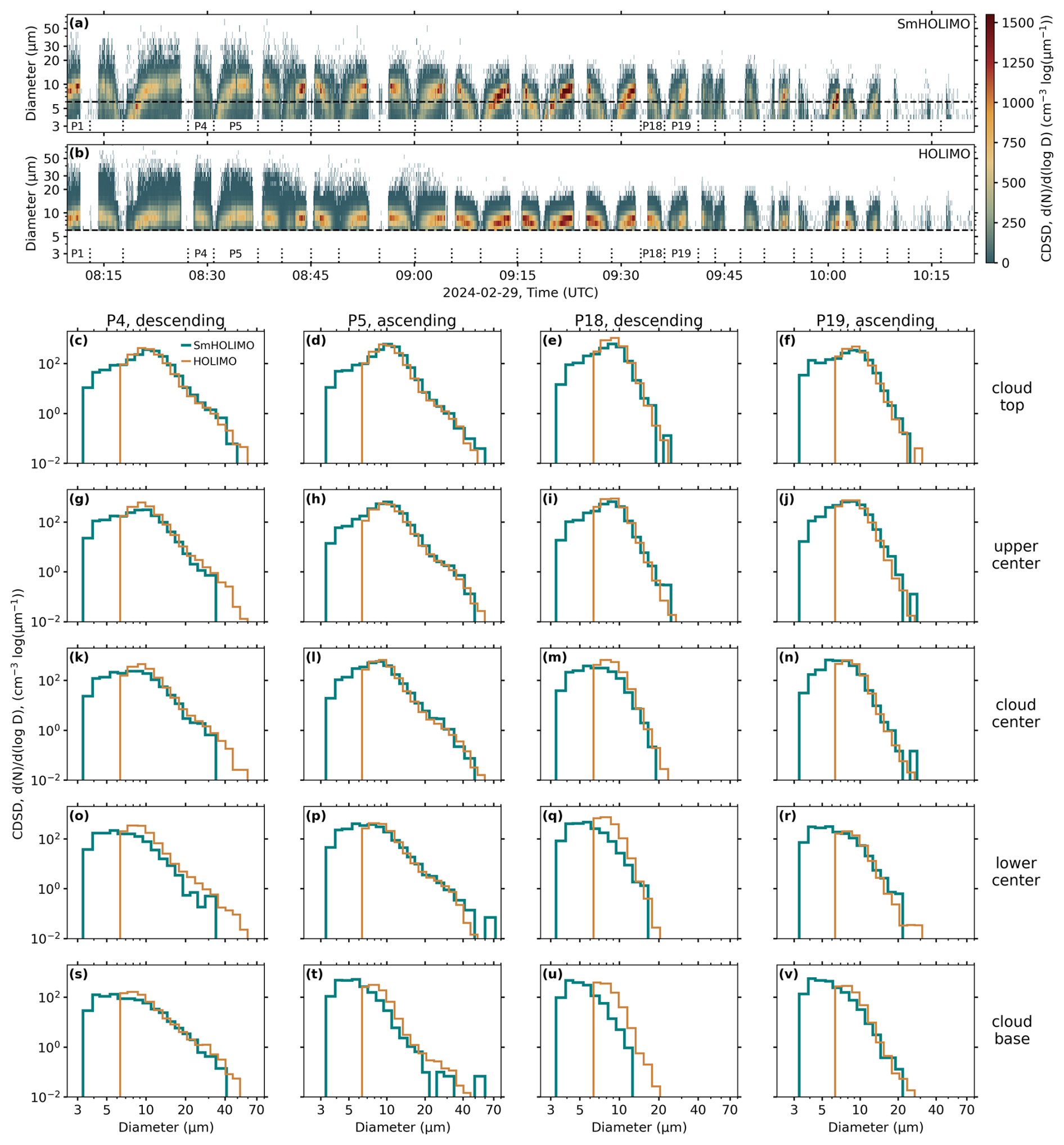
Figure 5 Cloud droplet size distributions (CDSDs) measured with SmHOLIMO (a) and HOLIMO (b) over time during the 30 profiles. The dotted black vertical lines at the bottom indicate the start and end of each profile. Exemplary profile numbers are shown for profiles P1, P4, P5, P18, and P19, with odd numbers representing ascending profiles and even numbers representing descending profiles (see Table B1). The resolution limit of HOLIMO, of 6 µm (dashed black line), is shown for easier comparison. Panels (c)–(v) show averaged CDSDs for different cloud sections with cloud top in row 1 (c–f), upper center in row 2 (g–j), cloud center in row 3 (k–n), lower center in row 4 (o–r), and cloud base in row 5 (s–v). The cloud sections are determined for each profile individually by dividing the observed total cloud thickness (constrained by LWC >0.01 g m⁻³) into five equally sized parts. Shown are profiles P4, descending, column 1 (c–s); P5, ascending, column 2 (d–t); P18, descending, column 3 (e–u); and P19, ascending, column 4 (f–v).

4.2 Meteorological conditions

On 29 February 2024, a low stratus cloud was present over the field site which dissipated over the course of the measurement period, as visible in the height–time indicator (HTI) radar reflectivity measurements shown in Fig. 4a, along with the flight level of the TBS showing the 30 profiles. A stable Bise situation (cold, dry, northeasterly winds), which generally facilitates the formation and the persistence of low stratus, weakened during the previous afternoon, due to a change in the synoptic weather situation. The wind direction and wind speed over the last 2 d (weather station on ground at field site) were ≈70° N and ≈5 m s⁻¹ and changed to variable wind directions and wind speeds between 1 and 2 m s⁻¹. The lack of solar radiation supported the low stratus to persist for another night, before the increase in radiation on the next morning led to its dissipation after 2 d of persistence. A more comprehensive work on the climatology and life cycle of wintertime low stratus in Switzerland can be found in Scherrer and Appenzeller (2014) and Westerhuis et al. (2020).

During the measurements, the cloud top decreased from 1500 to 1400 $\mathrm{m}\mathrm{a}.\mathrm{s}.\mathrm{l}.$, while the cloud base increased from 1150 to 1250 $\mathrm{m}\mathrm{a}.\mathrm{s}.\mathrm{l}.$ Around 09:00 UTC we observe a strong thinning of the cloud, and at about 09:45 UTC, the previously uniform cloud layer became increasingly patchy, visible in the HTI radar reflectivity measurements of Fig. 4a. Figure 4b and e show vertical profiles of meteorological parameters recorded by two radiosondes (RSs), RS1 and RS2, launched from the measurement site. A strong and stable temperature inversion is visible above cloud top (Fig. 4b and c). Due to the weakening/breakdown of the Bise situation, the wind speed was low, at about 2 m s⁻¹ below the inversion layer (Fig. 4d). The wind direction was variable over the measurement time period and altitude, covering directions from 0 to 150° N (Fig. 4e).

4.3 Cloud microphysical in situ observations: a comparison between SmHOLIMO and HOLIMO

The measured CDSDs of the 30 profiles are shown over time in Fig. 5a and b for SmHOLIMO and HOLIMO, respectively. Some exemplary profile numbers are shown, with odd numbered profiles being ascending and even numbered ones being descending (see Table B1). As intended, SmHOLIMO is capable of extending the observable size spectrum down to 3.7 µm, well below the resolution limit of HOLIMO at 6 µm (horizontal black dashed line), while still capturing the full upper end of the CDSD. Furthermore, SmHOLIMO observed the expected shift of the CDSD maxima towards larger cloud droplet diameters with increasing height inside the cloud, which is only faintly visible in the CDSDs measured with HOLIMO.

In Fig. 5c–v, we show averaged CDSDs of SmHOLIMO and HOLIMO for the four profiles P4, P5, P18, and P19, each divided into the five sections: cloud base, lower center, cloud center, upper center, and cloud top. The section ranges are based on the total vertical extent of the clouds (defined by LWC >0.01 g m⁻³) divided by 5 and are determined individually for each profile. The interpretation of the smallest size bins of the CDSD, for SmHOLIMO and HOLIMO, should generally be treated with caution as it is close to the respective resolution limit.

For the descending profiles, i.e., P4 and P18, we observe a deviation between the CDSDs measured by SmHOLIMO and HOLIMO, with SmHOLIMO measuring lower concentrations of larger cloud droplets and HOLIMO measuring higher concentrations of small droplets, especially in the cloud center and cloud base regions (e.g., Fig. 5k, m, o, q, and u). Our main hypothesis is that there are two interrelated reasons for this underestimation, namely the low atmospheric wind speed (≈2 m s⁻¹; see Fig. 4d) and the non-ideal mounting of SmHOLIMO on the measurement platform. The descending velocity of the TBS of ≈1 m s⁻¹ is close to the ambient wind speed, and SmHOLIMO was mounted on the measurement platform in the same orientation as shown in Fig. 1b with the sample volume above the electronics box. This combination resulted in non-isokinetic sampling of cloud droplets for descending profiles because the electronics box prevented an undisturbed airflow. In hindsight, the non-isokinetic sampling could easily have been avoided by turning SmHOLIMO by 90°, resulting in an unobstructed sample volume from above and below, as is the case for HOLIMO. Another hypothesis is that in the lower cloud and cloud base regions, some of the smaller cloud droplets may have been incorrectly sized by HOLIMO due to resolution limit effects, causing them to be assigned to a larger size bin, e.g., Fig. 5q and u. This feature persists across all cloud base region CDSDs (Fig. 5s–v), where HOLIMO generally measures higher concentrations in the smallest size bin compared to SmHOLIMO. However, as noted earlier, measurements in the smallest size bin should be interpreted with caution. Since the descending profiles are not trustworthy, we will discard them from the following analysis and focus on the data from ascending profiles only. To better assess the source of this discrepancy we conducted an intercomparison campaign at Mt. Sonnblick Observatory, Austria, between SmHOLIMO, HOLIMO, and the Fog Monitor (FM-120, Droplet Measurement Techniques, USA). The data are currently being analyzed.

The ascending profiles, i.e., P5 and P19, show very good agreement in CDSDs between SmHOLIMO and HOLIMO (Fig. 5, columns 2 and 4). The locations of the CDSD maxima show the expected shift from smaller sizes at the cloud base to larger sizes in the cloud top region. For the cloud top and upper center region (Fig. 5 row 1 and 2), both HOLIMO and SmHOLIMO are able to capture the full CDSD. We also want to emphasize that SmHOLIMO sufficiently captures droplets in the size range larger than 20 µm, despite the sample volume rate of 2.5 cm³ s⁻¹ that is more than 5 times smaller compared to HOLIMO's rate of 14 cm³ s⁻¹. However, starting from the cloud center region towards the cloud base (Fig. 5 row 3–5), we clearly see the importance of SmHOLIMO's ability to measure smaller cloud droplets down to 3.7 µm compared to 6 µm. As an example, in Fig. 5n in the cloud center region, we see how the CDSD measured with HOLIMO is truncated right at the maximum, giving a misleading location of the maximum at larger cloud droplet diameters, and this trend further intensifies toward the cloud base (see Fig. 5p and r). In the cloud base region (Fig. 5 row 5) it is particularly difficult to capture the full CDSD. Here, cloud droplets are formed and tend to have initial diameters in the submicron range, so even the low resolution limit of SmHOLIMO is not sufficient to capture the full CDSD, as can be seen in Fig. 5v. Nevertheless, and despite the seemingly marginal difference of 2.3 µm in resolution between HOLIMO and SmHOLIMO, SmHOLIMO provides a much more complete image of the CDSD.

The necessity of capturing a broad range of the CDSD becomes even more evident if we compare the derived quantities of CDNC, cloud droplet mean diameter, LWC, and cloud optical depth (τ_c) between SmHOLIMO and HOLIMO. They were obtained during the vertical profiles P5 and P19 (see Fig. 5) and are shown as absolute values in Fig. 6a–d and as ratios between SmHOLIMO and HOLIMO in Fig. 6e–h. P5 was measured while the cloud was still in a more stable phase, while P19 was obtained just before the breakup of the uniform cloud layer. Therefore, the trends over height for P5 are more consistent with the theory of an adiabatic cloud profile than the trends observed in P19. From an adiabatic cloud profile, we expect a rapid increase in CDNC near cloud base until it stabilizes to a more constant value after the height of maximum supersaturation is reached. We see how SmHOLIMO captures these features well during P5, while HOLIMO significantly underestimates the CDNC at lower cloud levels, measuring concentrations up to 4 times lower (Fig. 6a and e). Simultaneously, we expect a steady increase in cloud droplet mean diameter with height above cloud base. The increase in cloud droplet diameter from cloud base to cloud top is around 2.5 µm for SmHOLIMO and 1.3 µm for HOLIMO (Fig. 6b and f). Also, the retrieved mean diameters are up to 1.6 times smaller for SmHOLIMO in the cloud base region. Finally, we observe an almost linear increase in LWC with cloud height for both instruments during P5 (Fig. 6c), as expected for shallow clouds with vertical extents less than 1 km (Brenguier et al., 2011). The LWC measurements of SmHOLIMO and HOLIMO show an overall good agreement, with SmHOLIMO having slightly higher values in the cloud center and cloud top region. The similar LWCs indicate that it is mainly defined by the higher mass of the larger cloud droplets for the sampled low stratus, with small droplets having only a minor influence. In the cloud top region with larger mean diameters, with SmHOLIMO we observe a LWC that is 1.5 times higher (Fig. 6g). In contrast to the LWC, more and smaller droplets can have significant effects on the cloud optical depth already at cloud base (Fig. 6d and h). The optical depths ${\mathit{\tau }}_{\text{c,P5}}^{\ast }$ and ${\mathit{\tau }}_{\text{c,P19}}^{\ast }$ retrieved for the full cloud profiles are more than 10 % higher for SmHOLIMO. The differences would translate into attenuation of radiation that is 2.7 times and 1.2 times (Beer–Bouguer–Lambert law) higher obtained with SmHOLIMO for profile P5 and P19, respectively. The comparison between SmHOLIMO and HOLIMO measurements unequivocally shows the importance of capturing small cloud droplets in order to retrieve accurate cloud microphysical quantities to confirm or establish new hypotheses.

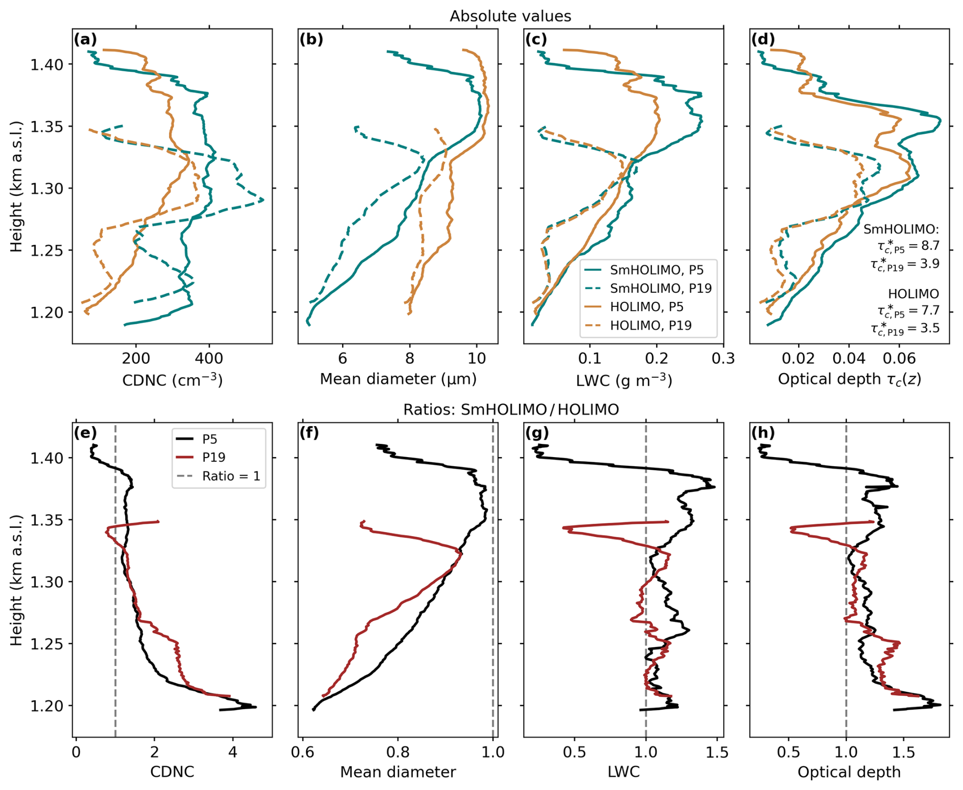
Figure 6 Absolute values of microphysical variables in (a)–(d) for SmHOLIMO (blue) and HOLIMO (orange) over height (in $\mathrm{km}\mathrm{a}.\mathrm{s}.\mathrm{l}.$). Shown are the ascending profiles P5 (solid) and P19 (dashed), also shown in Fig. 5. (a) Cloud droplet number concentration (CDNC) (in cm⁻³), (b) cloud droplet mean diameter (in µm), (c) liquid water content (LWC) (in g m⁻³), and (d) local cloud optical thickness τ_c(z) together with the full over height-integrated cloud optical thicknesses ${\mathit{\tau }}_{\mathrm{c}}^{\ast }=\int {\mathit{\tau }}_{\mathrm{c}}\left(z\right)\mathrm{d}z$. In (e)–(h) ratios (SmHOLIMO / HOLIMO) of cloud microphysical variable are shown for profile P5 (black) and P19 (red) for CDNC in (e), cloud droplet mean diameter in (f), LWC in (g), and cloud optical depth in (h). The 1 : 1 ratio is shown as a dashed gray line. A running mean over 20 s was applied to all data.

4.4 Comparison to remote sensing observations

The in situ observations are now compared against the remote sensing observations, i.e., a microwave radiometer (MWR, RPG-HATPRO-G5, RPG Radiometer physics GmbH, Germany) and a vertically pointing W-band Doppler cloud radar (RPG-FMCW-94, RPG Radiometer physics GmbH, Germany). In order to have a fair comparison between all data sets, we will only use SmHOLIMO and HOLIMO observations acquired during ascending profiles due to the sampling bias described in Sect. 4.3. The MWR and cloud radar are located at a horizontal distance of 100–150 m away from the in situ measurements (see Henneberger et al., 2023).

Figure 7a shows a time series of the liquid water path (LWP) measured by the MWR. The LWPs for SmHOLIMO and HOLIMO are determined by integrating the LWC over height for each ascending profile. The LWPs measured by SmHOLIMO and HOLIMO are in good agreement with the LWP observed by the MWR (i.e., they lie within the given uncertainty). Furthermore, all three measurements independently observe a sharp decrease in LWP around 09:30 UTC. The two linear regressions for SmHOLIMO and HOLIMO shown in Fig. 7b are in good agreement with the MWR data. Since their 95 % confidence intervals overlap and their respective slopes (SmHOLIMO: $(\mathrm{1.12}\pm \mathrm{0.07}){\mathrm{g}}^{-\mathrm{1}}{\mathrm{m}}^{\mathrm{2}}$; HOLIMO: $(\mathrm{1.05}\pm \mathrm{0.03}){\mathrm{g}}^{-\mathrm{1}}{\mathrm{m}}^{\mathrm{2}}$) agree within the given uncertainties, no significant differences can be inferred.

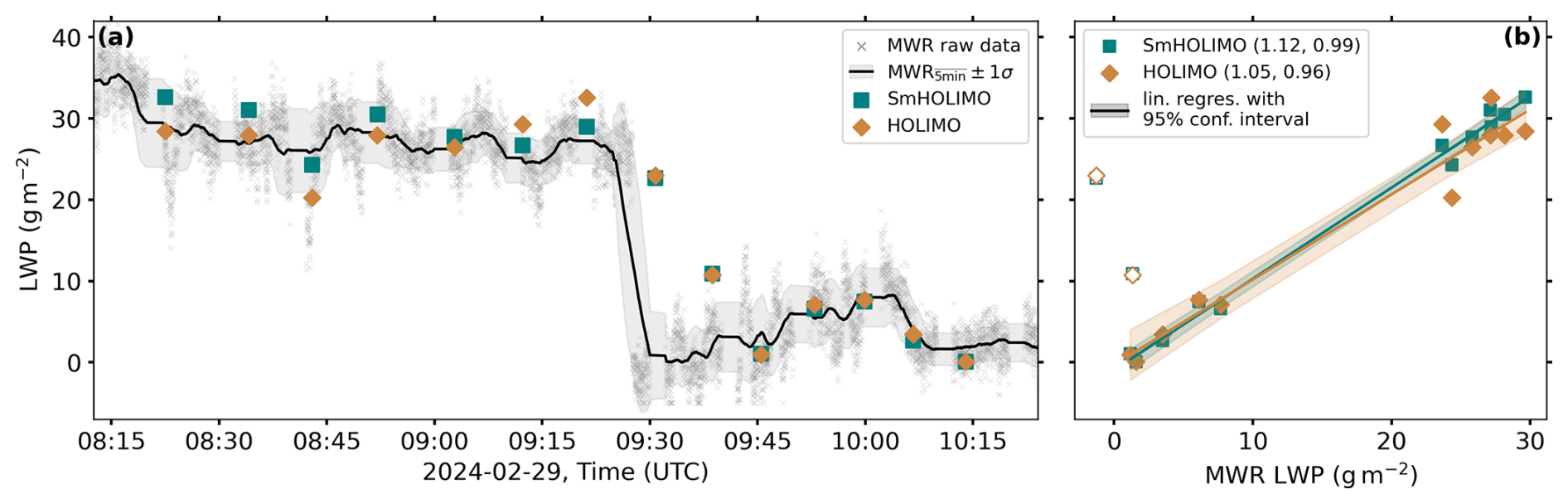
Figure 7 (a) Time series of the liquid water path (LWP) (in g m⁻²) observed with the Microwave Radiometer (MWR; gray crosses, raw data points) with a 5 min moving average (solid black) and the respective standard deviation (gray shading) together with the LWP derived from ascending profiles for SmHOLIMO (blue squares) and HOLIMO (orange diamonds). (b) Correlation plot of SmHOLIMO (blue) and HOLIMO (orange) LWPs vs. MWR LWPs. Also shown are linear regressions (solid lines) with respective slopes and Pearson r² values in parentheses (slope, r²) and 95 % confidence intervals (shading). The unfilled data points obtained between 09:30 and 09:45 UTC were excluded from the linear regression due to a strong spatial inhomogeneity in the air mass.

Finally, we compared the in situ observations of SmHOLIMO and HOLIMO with the equivalent reflectivities measured by the cloud radar. To do this, we approximate the equivalent in situ equivalent reflectivities (in dBZ) by converting the measured CDSDs first into the radar reflectivity Z using the discretized radar equation

$$Z=\mathrm{64}\sum _{i}N\left(r_i\right)\cdot r_i^{\mathrm{6}},$$

with N(r_i) the cloud droplet size distribution as concentrations per bin, r_i the mean radius of each size bin, and i the number of size bins. The equivalent reflectivity Z_e is then calculated using

$$Z_{\mathrm{e}}={\displaystyle \frac{|K{|}^{\mathrm{2}}}{\mathrm{0.93}}}\cdot \mathrm{10}\cdot {\log }_{\mathrm{10}}\left({\displaystyle \frac{Z}{\mathrm{1}{\mathrm{mm}}^{\mathrm{6}}{\mathrm{m}}^{-\mathrm{3}}}}\right),$$

with $|K{|}^{\mathrm{2}}=\mathrm{0.93}$, the square of the absolute value of the complex index of refraction for liquid particles.

The temporal evolution of the Z_e is shown in Fig. 8a–c for the radar, SmHOLIMO and HOLIMO. For the in situ observations only values $Z_{\mathrm{e}}>-\mathrm{60}\mathrm{dBZ}$ are shown, which corresponds to the lower limit for the cloud radar. A qualitative comparison of Fig. 8b and c with the HTI radar measurements in Fig. 8a shows a good agreement for all ascending profiles and a clear underestimation of the Z_e for the descending profiles of SmHOLIMO due to the sampling bias described in Sect. 4.3. Correlation plots of the calculated in situ Z_e vs. the measured radar Z_e are shown in Fig. 8d and e for ascending profiles. Based on linear regressions we observe better agreement for the SmHOLIMO data with a slope of 0.82±0.03 compared to HOLIMO 0.66±0.02. In general, one observes a larger spread of data points below the 1 : 1 line, indicating a more pronounced underestimation of Z_e by the in situ measurements, in particular for SmHOLIMO. This bias arises directly from the large difference in the observed cloud volume, which is more than 7 orders of magnitude higher for the radar data points with >1000 m³ compared to <0.1 L for the in situ measurements. Since Z_e is dominated by the largest droplets ($\propto r_i^{\mathrm{6}}$), we believe that this underestimation results from the lower probability of observing large droplets since they occur less frequently.

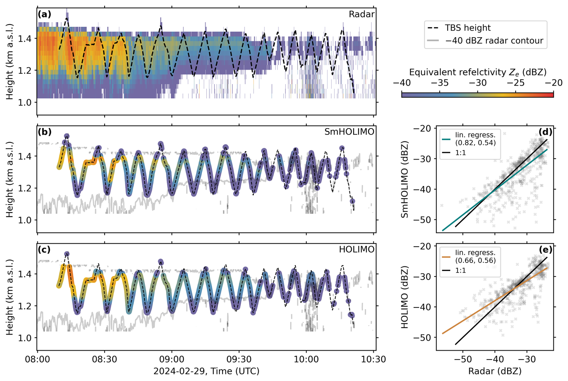
Figure 8 (a) Measured height–time indicator (HTI) equivalent reflectivities Z_e (in dBZ) from a vertically pointing W-band Doppler cloud radar. Calculated Z_e (in dBZ) over the TBS flight track for SmHOLIMO in (b) and HOLIMO in (c), together with the −40 dBZ contour line (gray lines) from the radar Z_e measured in (a). Calculated reflectivities are shown only for values $>-\mathrm{60}$ dBZ (lower limit of cloud radar). A moving average over 20 s is applied to the calculated Z_e in (b) and (c). Correlation plots of the calculated Z_e vs. the radar Z_e (gray crosses) are shown in (d) for SmHOLIMO and (e) for HOLIMO. Also shown are the 1 : 1 lines (solid black) and linear regressions (solid blue, d, solid orange e) with slopes and Pearson r² values in parentheses (slope, r²).

5 Conclusions

This study demonstrates the successful application of SmHOLIMO, a newly developed holographic cloud particle imager. SmHOLIMO's resolution limit of 3.7 µm approaches the limits of forward-scattering probes and is sufficiently small to capture key liquid phase cloud microphysical properties, such as number concentration, mean droplet diameter, and optical depth, in regions with small droplets (e.g., cloud base regions, continental clouds), while being still capable to capture large droplets (e.g., drizzle). The open-path holographic setup further retains the fundamental benefits of holography such as (1) a well-defined sample volume, which is unaffected by inflow velocities and does not require a moving platform; (2) reduced effects of non-isokinetic sampling of cloud particles, since no inlets and suction pumps are required; (3) independence of size, phase, refractive index, and shape of cloud particles; and (4) facilitation of spatial analyses. After a successful characterization, i.e., the resolution and droplet sizing tests of SmHOLIMO in the laboratory, the instrument was deployed in the field. A dissipating low stratus cloud was probed on 29 February 2024 by 29 vertical profiles using a TBS.

SmHOLIMO is a specialized in situ instrument within the field of holographic imagers. Unlike other holographic imagers (e.g., HOLIMO or HOLODEC) designed to capture both cloud droplets and ice crystals, SmHOLIMO is specifically optimized for detecting small cloud droplets, thereby trading sample volume for resolution. Scientific applications of SmHOLIMO include the precise measurements of liquid-phase cloud microphysical properties from highly localized cloud volumes (0.5 cm³) using single holograms. This enables the study of small-scale features that would otherwise be lost when averaging over larger cloud sections (Beals et al., 2015). In liquid-phase clouds, this capability is particularly valuable for characterizing transient regions such as cloud edges, where entrainment can cause droplets to shrink or to completely evaporate. This entrainment can result in homogeneous or inhomogeneous mixing (Korolev et al., 2016) and thereby lead to the formation of cloud droplet voids and filament structures. Similarly, at cloud base regions, SmHOLIMO can provide insights into the initial stages of cloud droplet formation.

In mixed-phase clouds, SmHOLIMO can complement a “standard” holographic imager (e.g., HOLIMO) in a co-located setup to investigate transitions between fully liquid and fully glaciated regions. This setup is particularly useful for studying how the ice phase influences the liquid phase, improving the discrimination between genuinely (cloud droplets and ice appear homogeneously mixed) and conditionally (cloud droplets and ice crystals appear in separated pockets) mixed-phase clouds (see Korolev et al., 2017). A specific example, where such a setup would have been beneficial is the CLOUDLAB project (Henneberger et al., 2023), which investigated the Wegener–Bergeron–Findeisen (WBF) process (Wegener, 1911; Bergeron, 1935; Findeisen, 1938) through glaciogenic cloud seeding experiments. In situ observations from HOLIMO showed that transitions between fully liquid and (apparently) fully glaciated cloud sections occur on scales of <10 m. However, since HOLIMO can only resolve droplets down to 6 µm, it remains uncertain whether these cloud regions were truly free of cloud droplets or whether the WBF process had reduced droplet sizes below the detection threshold of HOLIMO (6 µm). SmHOLIMO, with its enhanced resolution, could have helped to better constrain this ambiguity.

First, we compared the results of SmHOLIMO with those of another holographic imager, HOLIMO, probing the same cloud. Here, the unfortunate mounting of SmHOLIMO on the measurement platform, with the sample volume being blocked from below, resulted in undersampling of larger cloud droplets for descending profiles, which were subsequently excluded from most of the analysis. For the ascending profiles we conclude that the small sampling volume rate of 2.5 mL s⁻¹ compared to 14 mL s⁻¹ for HOLIMO is sufficient to capture the main features of the CDSD, including the upper tail of the size distribution. For the cloud base region, we emphasize the importance of measuring small cloud droplets. Despite the seemingly marginal difference of 2.3 µm in resolution between SmHOLIMO and HOLIMO, the CDNC of HOLIMO was underestimated by a factor of up to 4, and the mean cloud droplet diameter was overestimated by a factor of up to 1.6 compared to SmHOLIMO data. Inherently, the cloud optical depth is increased by 10 % for SmHOLIMO due to the larger integrated cloud droplet surface area, which translates into an attenuation of radiation that is up to 2.7 times higher.

Finally, we also compared the in situ observations of liquid water path (LWP) and derived equivalent radar reflectivity Z_e with remote sensing measurements of a microwave radiometer (MWR) and a cloud radar, respectively. The LWPs derived from the in situ data resemble MWR data, and no significant difference was found between the two in situ observations. The trends of Z_e calculated from the in situ instruments follow the remotely sensed Z_e but tended to underestimate them in general. From linear regressions we find that SmHOLIMO shows better agreement with the cloud radar data than HOLIMO (slope closer to unity). Conversely, we see that Z_e obtained from HOLIMO data has a more homogeneous distribution around the unity line, while for SmHOLIMO a stronger bias towards underestimating Z_e is visible, which could be an effect of the smaller sampling volume.

In summary, this study has demonstrated the capabilities of SmHOLIMO to perform precise in situ measurements of cloud droplets down to 3.7 µm in diameter and has shown the importance of being able to measure a broad size spectrum with emphasis on small cloud particles in order to accurately determine cloud microphysical variables.

Appendix A: Sample volume and droplet sizing

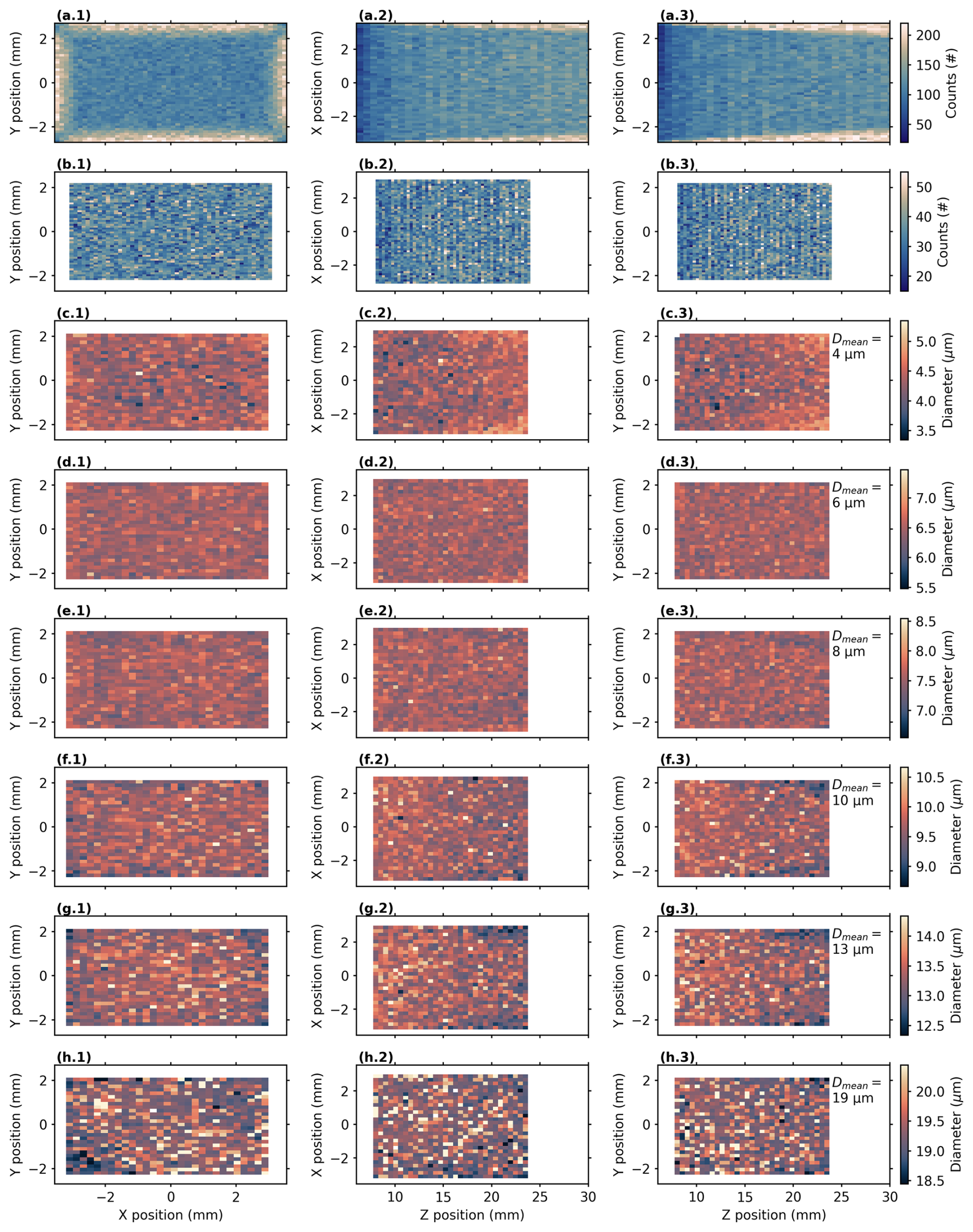
Figure A1 Multi-view orthographic projection of the SmHOLIMO sample volume with the XY plane in (a.1)–(h.1), the XZ plane in (a.2)–(h.2), and the YZ plane in (a.3)–(h.3). Panels (a.1)–(b.3) show the droplet count distributions over the sample volume for all droplet locations retrieved during the calibration of the sizing algorithm in Sect. 3.2. The count distributions over the full (untrimmed) sample volume ($-\mathrm{3.55}<X<\mathrm{3.55}$, $-\mathrm{2.7}<Y<\mathrm{2.7}$, and $\mathrm{6}<Z<\mathrm{30}$ mm) are shown in (a.1)–(a.3). A non-uniform distribution is visible with increasing droplet number towards the outer edges of the volume. This, in holography, well-known edge effect results from an incomplete capture of the wavefront at the edges of the camera sensor and an increase in the signal-to-noise ratio with increasing Z positions. A uniform count distribution is achieved after reducing the sample volume to $-\mathrm{3.1}<X<\mathrm{3.1}$, $-\mathrm{2.2}<Y<\mathrm{2.2}$, and $\mathrm{8}<Z<\mathrm{24}$ mm, as shown in (b.1)–(b.3). Panels (c.1)–(h.3) show the results of the droplet sizing algorithm over the trimmed sample volume for the six different droplet sizes (diameters in (c.3)–(h.3)) generated during the sizing calibration in Sect. 3.2. Generally sufficient uniform sizing is achieved for all droplet diameters, with small deviations for larger Z positions Z>20 mm. Scientific color maps created by Crameri (2023).

Appendix B: Table of profile data

Table B1 Overview of the 29 profiles taken during the case study on 29 February 2024. The number of analyzed holograms (holo. no) and the corresponding sampled volume are given for in cloud conditions (LWC >0.01 g m⁻³). Note that P1 is a half profile; see Fig. 4a.

Appendix C: Uncertainties in cloud droplet size distributions

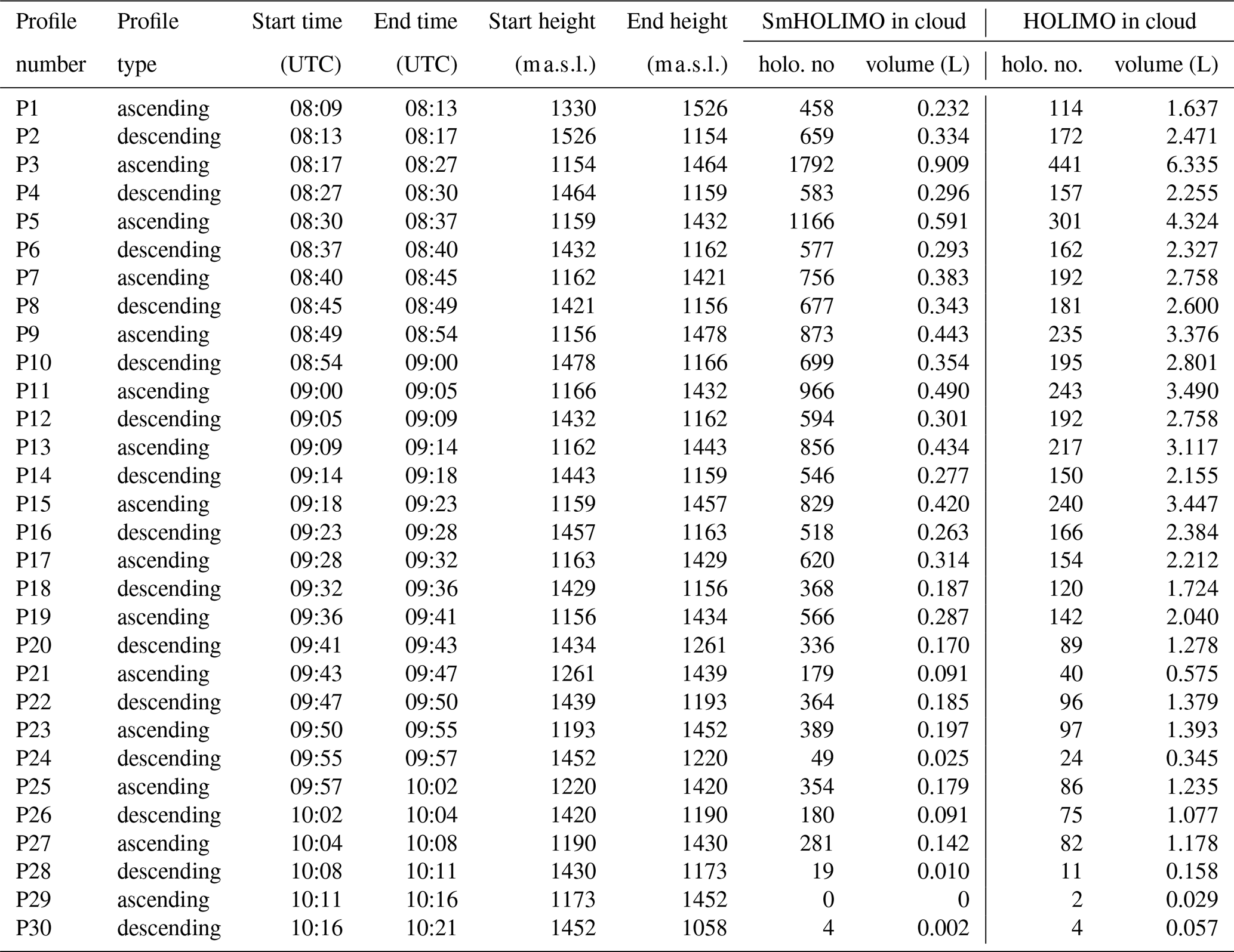
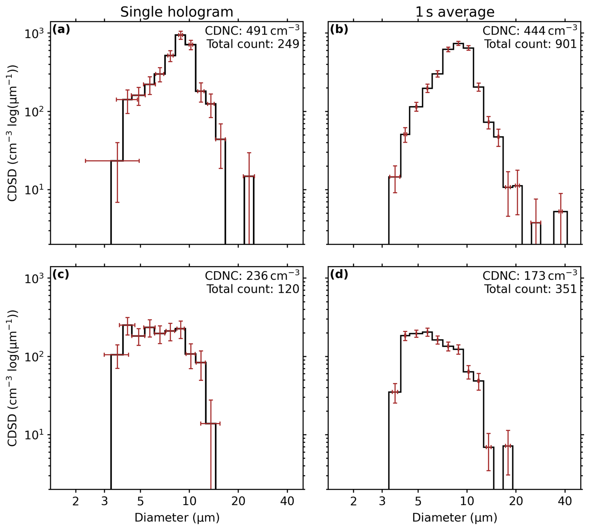
Figure C1 Exemplary cloud droplet size distributions (CDSDs) measured with SmHOLIMO in black with associated diameter and counting uncertainties (red error bars). Panels (a) and (c) show CDSDs retrieved from single holograms recorded at 08:09:59.736 UTC and 08:39:59.955 UTC, respectively. Panels (b) and (d) show CDSDs averaged over 1 s intervals, recorded between 08:09:59–08:10:00 UTC and 08:39:59–08:40:00 UTC, respectively. Diameter uncertainties are calculated as $\mathrm{\Delta }d=d_{\mathrm{s}}\cdot {\sqrt{N}}^{-\mathrm{1}}$, with d_s=1.85 µm the error of a single droplet measurement of pixel pitch and N being the number of droplets in each size bin. Counting uncertainties are derived from counting statistics as $\sqrt{N}$. The CDNC and respective total number of droplets are indicated in the upper-right corner of each panel.