Development of a forced advection sampling technique (FAST) for quantification of methane emissions from orphaned wells

Orphaned wells, meaning unplugged and non-producing wells lacking responsible owners, pose a significant and undersampled environmental challenge due to their vast number and unknown associated emissions. We propose, develop and test an alternative method for estimating emissions from orphaned wells using a forced advection sampling technique (FAST) that can overcome many of the limitations in current methods (cost, accuracy, safety). In contrast to existing ambient Gaussian plume methods, our approach uses a fan-generated flow to force advection between the emission source and a point methane (CH₄) sensor. The fan flow field is characterized using a colocated sonic anemometer to measure the 3D wind profile generated by the fan. Using time-series measurements of CH₄ concentration and wind, a simple estimate of the CH₄ emission rate of the source can be inferred. The method was calibrated using outdoor controlled-release experiments and then tested on four orphaned wells in Lufkin, TX, and Osage County, OK. Our results suggest that the FAST method can provide a low-cost, portable, fast and safe alternative to existing methods with reasonable estimates of orphaned well emissions over a range of leak rates below 40 g h⁻¹ and within certain geometric and atmospheric constraints.

1 Introduction

1.1 Motivation

Orphaned oil and gas wells, meaning unplugged and non-producing wells lacking responsible owners, pose a significant and undersampled environmental challenge. In the United States (US) alone, there are approximately 120 000 documented orphaned wells (Merrill et al., 2023), with an estimated 310 000 to 800 000 more undocumented wells (IOGCC, 2021). For much of the 20th century, orphaned wells were considered a non-issue compared to active wells, as they were thought to have low emission rates, particularly when they were reported as “plugged”. However, existing estimates of total orphaned well emissions are based only on direct measurements of < 0.03 % of known wells (Kang et al., 2023), making them a highly undersampled and uncertain source of anthropogenic methane (CH₄). CH₄ is a potent greenhouse gas with a global warming potential (GWP) 84 times higher than carbon dioxide (CO₂) taken over 20 years (IEA, 2025) and a relatively short lifetime (8–11 years), making it a high priority in combating near-term global warming. Based on a database of leak measurements at 598 wells across the US and Canada, it was found that “annual methane emissions from abandoned wells are underestimated by 150 % in Canada and by 20 % in the U.S.” (Williams et al., 2021). This lack of reliable emission data has resulted in increased interest in measuring and plugging orphaned wells as an important area of research for methane emissions reduction and near-term climate change mitigation (O'Malley et al., 2024).

Alongside academia, the political sphere has shown increased interest in measuring and plugging orphaned wells. The Global Methane Pledge was signed at COP26 in 2021 by 155 countries representing over 50 % of global CH₄ emissions who committed to 30 % reductions in emissions from 2020 levels by 2030 (UNFCCC Secretariat, 2022). The US has since begun to investigate plugging orphaned wells, with an investment of USD 660 million in 2023 through the Department of Interior (U.S. DOI, 2023). From 2018–2020, the average cost of plugging a single well in the US ranged from USD 2400 to 227 000, with an overall 3-year average of USD 25 634 (IOGCC, 2021). Using these numbers directly, without adjusting for inflation or overhead costs, this funding would be sufficient for plugging around 25 000 wells, or only 20 % of the documented orphaned wells and a mere 3 % of the upper bound of total orphaned wells. Given the high-cost of surveying and plugging, it will be critical to prioritize wells with larger emissions to reduce the economic burden of plugging orphaned wells.

Estimating emissions from orphaned wells is challenging due to their remote locations and typically low emission rates (Riddick et al., 2020; Saint-Vincent et al., 2020). Based on the aforementioned database of 598 wells across the US and Canada, it has been estimated that orphaned well emission rates range from less than 1 to 48 g h⁻¹ per well, with an average of around 6 g h⁻¹ (Williams et al., 2021). However, recent measurements in the US have also shown abandoned orphaned well emissions exceeding 1 kg h⁻¹ with a mean value of 138 g h⁻¹ (Follansbee et al., 2024; Riddick et al., 2024). Still, extremely high-emitting orphaned wells are very rare, and the vast majority of wells emit below the thresholds needed to observe them using current remote sensing platforms (Sherwin et al., 2024).

There are a variety of ground-based measurement approaches that can be applied to measure emissions from orphaned wells (Table 1). These range from expensive hand-held forward-looking infrared (FLIR) cameras to more time-intensive mobile (OTM-33a) (U.S. EPA, 2014) and stationary systems (SEMTECH Hi-Flow 2 – SEMTECH, 2024; Chamber – Williams et al., 2023; Gaussian plume modeling, GPM – Lushi and Stockie, 2010; Vent – Ventbusters, 2023). Uncrewed aerial vehicles (UAVs, also known as “drones”) have also recently been proposed as a means of measuring wells, and preliminary results look promising (Dooley et al., 2024). However, due to the expensive or complex nature of most of these methods only < 0.03 % of orphaned wells have been sampled. To overcome this data gap, new robust and fast techniques for estimating emission rates on the order of 1 g h⁻¹ to tens of grams per hour are needed (i.e. FAST).

Table 1 Comparative assessment of commercial (FLIR, SEMTECH Hi-Flow 2, Vent) and research (Chamber, GPM, UAV, OTM-33a) methods used to monitor fugitive methane leaks from orphaned wells. Hardware costs, detection range, accuracy, size, labor and safety are compared for each technology.

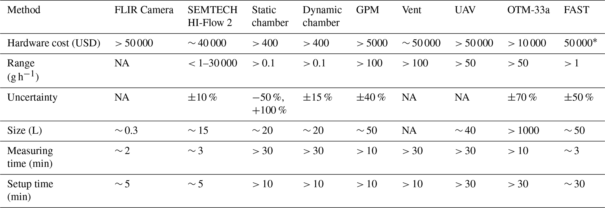
^* The FAST method in this study is currently limited by the high cost of laser trace gas sensors (Picarro, Aeris, etc.) that can be reduced significantly by using cheaper non-laser sensors (i.e. Gas Rover) used in chambers. NA: not available.

Previous studies have investigated existing methods for quantifying methane emissions on the order of those relevant for studying orphaned wells (Dubey et al., 2023; Riddick et al., 2023, 2022). Table 1 shows a list of the existing technologies that can measure methane emissions in this regime and their relative costs and sensitivities. The existing methods that are accurate and portable enough for measuring orphaned wells have other limitations, including insensitivity (FLIR), high-cost (SEMTECH), complexity and safety (Chamber – Riddick et al., 2023; Vent – Ventbusters, 2023; UAV – Dooley et al., 2024; OTM-33a – Edie et al., 2020), accuracy, hardware and labor costs that are summarized in Table 1. Therefore, there is a pressing need for a cost-effective, efficient, safe and accurate method using existing sensors to estimate methane emissions for prioritizing orphaned well plugging. Although the FAST method is currently relatively expensive and difficult to set up/transport, it could be considered safer than many approaches, will work in complex aerodynamic environments, and could be used to quantify emissions from larger pieces of infrastructure such as abandoned pump jack wells that will not fit in a chamber or are surrounded by trees.

In this paper, we propose, develop and test a novel method for estimating CH₄ emissions from orphaned wells using a forced advection sampling technique (FAST) that can overcome many of the limitations of other methods, as outlined in Table 1. In contrast to existing ambient Gaussian plume modeling (GPM) methods, our approach uses a fan-generated flow to force advection between the emission source and a point sensor. This eliminates the need for an estimate of atmospheric stability, which is required to use the GPM. Using a colocated anemometer to measure the 3D wind profile generated by the fan, a simple estimate of the CH₄ emission rate of the source can be obtained. The method is calibrated using an outdoor controlled-release experiment and blindly tested on four wells in Lufkin, TX, and Osage County, OK. We report results that suggest that the FAST method can potentially provide a low-cost, portable, fast and safe alternative to existing methods to provide reasonable estimates of orphaned well emissions under reasonable meteorological conditions.

1.2 Mathematical model

The physics underlying the FAST approach are based on a steady-state solution to the advection–diffusion equation. This solution, known as the Gaussian plume equation (Veigele and Head, 1978), has been widely used in the literature to perform emission inversions. However, previous studies using the Gaussian plume equation consider larger emission sources and length scales (> 2 m) than those of interest in this study (Snoun et al., 2023; Perry et al., 2005). As a result, traditional GPM studies are typically dependent on parametrizations (i.e. Pasquill stability class), which are too coarse for the length scale and timescale used when studying orphaned wells at smaller (on the order of a meter) length scales. Furthermore, most previous studies using the GPM approach use ambient winds as opposed to a fan-generated plume within an ambient background. In one exception to this, an approach to localize emissions using a fan-generated flow was devised by Sánchez-Sosa et al. (2018). However this approach was only tested indoors and did not estimate emissions for their source of interest (ethanol).

Here we outline the underlying physics of scalar transport within a jet of fan-generated turbulent flow and derive a linear equation that can be used to estimate the emission rate of a source from time-averaged centerline measurements of concentration and wind velocity within that flow.

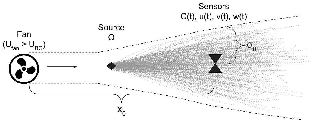
Figure 1 Schematic of the FAST method where an upwind fan (with mean downwind speed U_fan larger than the background U_BG) generates a turbulent jet to advect a non-reactive gas (CH₄) leaking at volumetric flow rate (Q) from a source to downwind sensors (anemometer measuring u(t), v(t) and w(t) and CH₄ analyzer measuring C(t)).

The method assumes a constant emission source with emission rate Q (g s⁻¹) positioned downstream of a fan aligned with the mean background wind direction, where the velocity of the fan flow (U_fan) is larger than that of the background wind (U_BG). Adding this fan creates an environment which is assumed to have homogeneous turbulence between the source and the sensors. The sensors are positioned downstream along the centerline from the fan by a distance (x₀) and measure time series of concentration (C) and velocity (u, v, w).

The estimated emission rate ($\widehat{Q}$) is calculated by integrating the scalar flux (C⋅u) over a circular cross-section (dA) at some downstream location.

$$\begin{array}{}\text{(1)}& \begin{array}{l}Q=\oint Cu\mathrm{d}A\approx \underset{\mathrm{¯}}{C_{\mathrm{CL}}}\underset{\mathrm{¯}}{u_{\mathrm{CL}}}\mathit{\pi }{\mathit{\sigma }}_{\mathrm{0}}^{\mathrm{2}},\\ \widehat{Q}=\underset{\mathrm{¯}}{C_{\mathrm{CL}}}\underset{\mathrm{¯}}{u_{\mathrm{CL}}}\mathit{\pi }{\mathit{\sigma }}_{\mathrm{0}}^{\mathrm{2}},\end{array}\end{array}$$

where spatial averages of concentration and velocity are approximated with time averages (underline) of centerline measurements (subscript “CL”). This gives a radial distance (σ₀) which is approximately the effective width of the plume at the downwind distance x₀. This radial distance σ₀ is estimated based on a previous study of fan-generated flows (Halloran et al., 2014) as a form of turbulent transport (Taylor, 1922). Halloran et al. (2014) showed that the expansion of a fan-generated plume close to the source is proportional to the square root of the downwind distance and dependent on the turbulence intensity (i_fan) and characteristic length scale (l_fan) of the fan.

$$\begin{array}{}\text{(2)}& \begin{array}{l}\mathit{\sigma }\sim {\left(i_{\mathrm{fan}}{l}_{\mathrm{fan}}x\right)}^{\frac{\mathrm{1}}{\mathrm{2}}}\\ {\mathit{\sigma }}_{\mathrm{0}}={\left(\mathit{\beta }{i}_{\mathrm{fan}}{l}_{\mathrm{fan}}{x}_{\mathrm{0}}\right)}^{\frac{\mathrm{1}}{\mathrm{2}}}\end{array}\end{array}$$

Evaluating Eq. (2) at location x₀ and combining with Eq. (1), $\widehat{Q}$ can be rewritten as a linear function of time-averaged centerline concentration and velocity measurements:

$$\begin{array}{}\text{(3)}& \widehat{Q}=\mathit{\pi }\mathit{\beta }{i}_{\mathrm{fan}}{l}_{\mathrm{fan}}{x}_{\mathrm{0}}\underset{\mathrm{¯}}{C_{\mathrm{CL}}}\underset{\mathrm{¯}}{u_{\mathrm{CL}}}=K_{\mathrm{FAST}}\underset{\mathrm{¯}}{C_{\mathrm{CL}}}\underset{\mathrm{¯}}{u_{\mathrm{CL}}},\end{array}$$

where the proportionality constant (K_FAST) is only dependent on constants related to the fan and the geometry of the system β (which is treated in more detail in Appendix A).

$$\begin{array}{}\text{(4)}& K_{\mathrm{FAST}}=\mathit{\pi }{\mathit{\sigma }}_{\mathrm{0}}^{\mathrm{2}}=\mathit{\pi }\mathit{\beta }{i}_{\mathrm{fan}}{l}_{\mathrm{fan}}{x}_{\mathrm{0}}\end{array}$$

2 Methods

2.1 Fan characterization experiments

To characterize the effectiveness of using a fan to generate a turbulent jet for the FAST method, experiments were conducted at Lawrence Berkeley National Lab (LBNL) on the afternoon of 16 April 2024 and in the morning of 21 May 2024 (Fig. 2). For both experiments, a Gill Windmaster (United Kingdom) 3D sonic anemometer was used to collect 3D wind speed measurements at 10 Hz downwind of a Minneapolis Duct Blaster (MDB) fan with no attachments. This fan was chosen as it is similar to those used in Halloran et al. (2014) and can be easily operated in the field at multiple fan speeds controlled by a dial. Both the fan and the anemometer were mounted on tripods at a height of 1 m. For these experiments, u is aligned to be in the x direction (upwind/downwind), v in the y direction (crosswind) and w in the z direction (vertical).

A key assumption of this study is that the effective plume width (σ₀) derived in Halloran et al. (2014) for smoking oil plumes is applicable to methane dispersion from orphaned wells. While the MDB fan generates turbulent transport similar to Halloran et al. (2014), differences in the physical properties of smoking oil and methane – such as buoyancy, diffusion rates and emission dynamics – could lead to deviations in plume behavior. These potential differences underscore the need for additional experiments designed specifically for methane to validate the use of σ₀ under these conditions and further refine the FAST method's applicability.

During the first experiment, measurements were taken for 9 min intervals at downwind distances of 0.5–5 m for two different fan speed settings, referred to as “low” (∼ 3 m s⁻¹ on average at a distance of 1 m) and “high” (∼ 5 m s⁻¹ on average at a distance of 1 m). The system was set up to be aligned to the background wind of ∼ 3 m s⁻¹ from west-northwest. Despite attempts to align the fan with the dominant background wind direction, there were still persistent crosswind gusts on the order of ∼ 1 m s⁻¹ which varied as the experiment progressed. Moreover, the vertical velocity (w) was higher than expected for two main reasons: the anemometer is mounted at a height of 1 m and the experiment was conducted on a rooftop. While w should be ∼ 0 m s⁻¹ at ground level, we measured w on the order of ∼ 1 m s⁻¹ due to these factors.

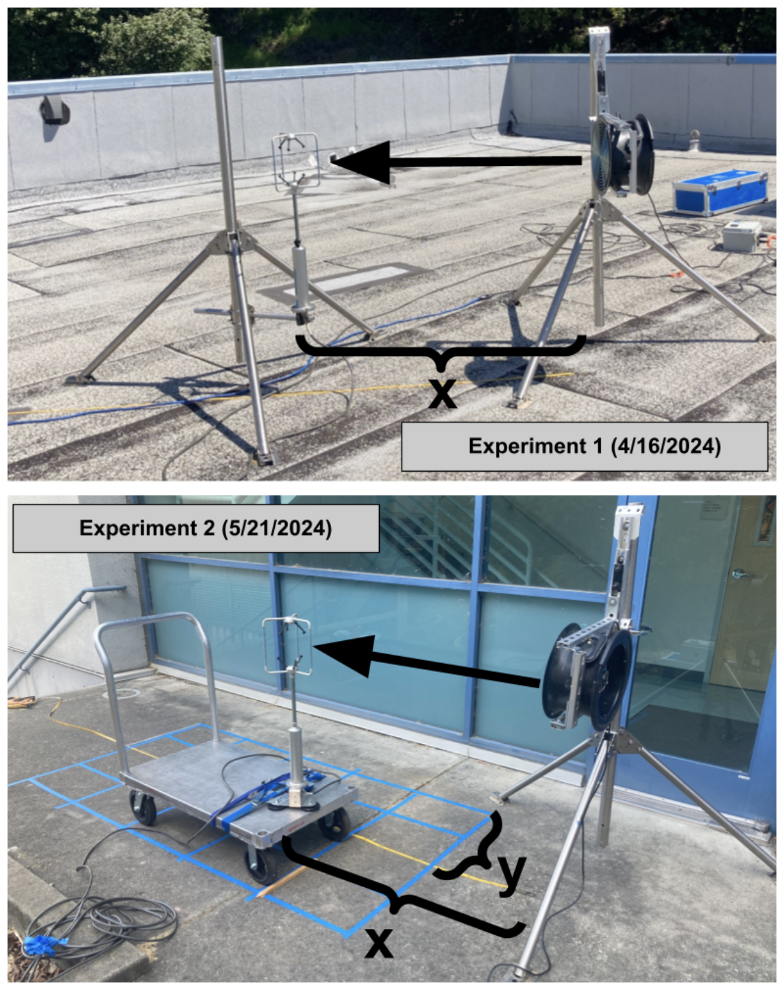
Figure 2 Experimental setup for fan characterization experiments using an anemometer placed at a downwind distance x and crosswind distance y (second experiment).

2.2 Controlled-release experiment

To verify and estimate the relevant parameters used in the FAST method, a controlled-release experiment was conducted using a range of constant methane leak rates. The SEMTECH HI-FLOW backpack system was used for verification as it has already been validated as a commercial product for estimating leak rates (see Appendix B for more details).

2.2.1 Experimental setup

The fan position, source position and sampling position were all 1 m above ground level and separated from each other by 1 m along an axis parallel to the ground, with the source placed in between the fan and the sample point (Fig. 3). A methane source was prepared by mixing 75 psi (0.517 MPa) of high-purity CH₄ with 1425 psi (9.825 MPa) ultra-high-purity N₂ in a 30 L aluminum cylinder to obtain a blend of 5.0 ± 0.17 %. The source was released from the cylinder at controlled rates using a regulator plumbed through a mass flow controller (Brooks Instrument GF40) programmed with set points corresponding to planned CH₄ emission rates of 1, 2, 5, 10, 20 and 40 g h⁻¹. The sampling for the FAST method was conducted using a Picarro G4302 analyzer (GasScouterTM G4302 Mobile Gas Concentration Analyzer; Picarro, 2025) for measuring the CH₄ concentration and a Gill Windmaster 3D sonic anemometer placed as physically close together as possible at the sample position (inlet tube mounted within 1 cm of center of anemometer; see Fig. 3 and Table 2). The forced advection was done using an MDB fan with no attachments. The fan, anemometer and data collection systems were powered using a 300 Ah 12 V DC battery and inverter, while the Picarro analyzer ran on its internal battery.

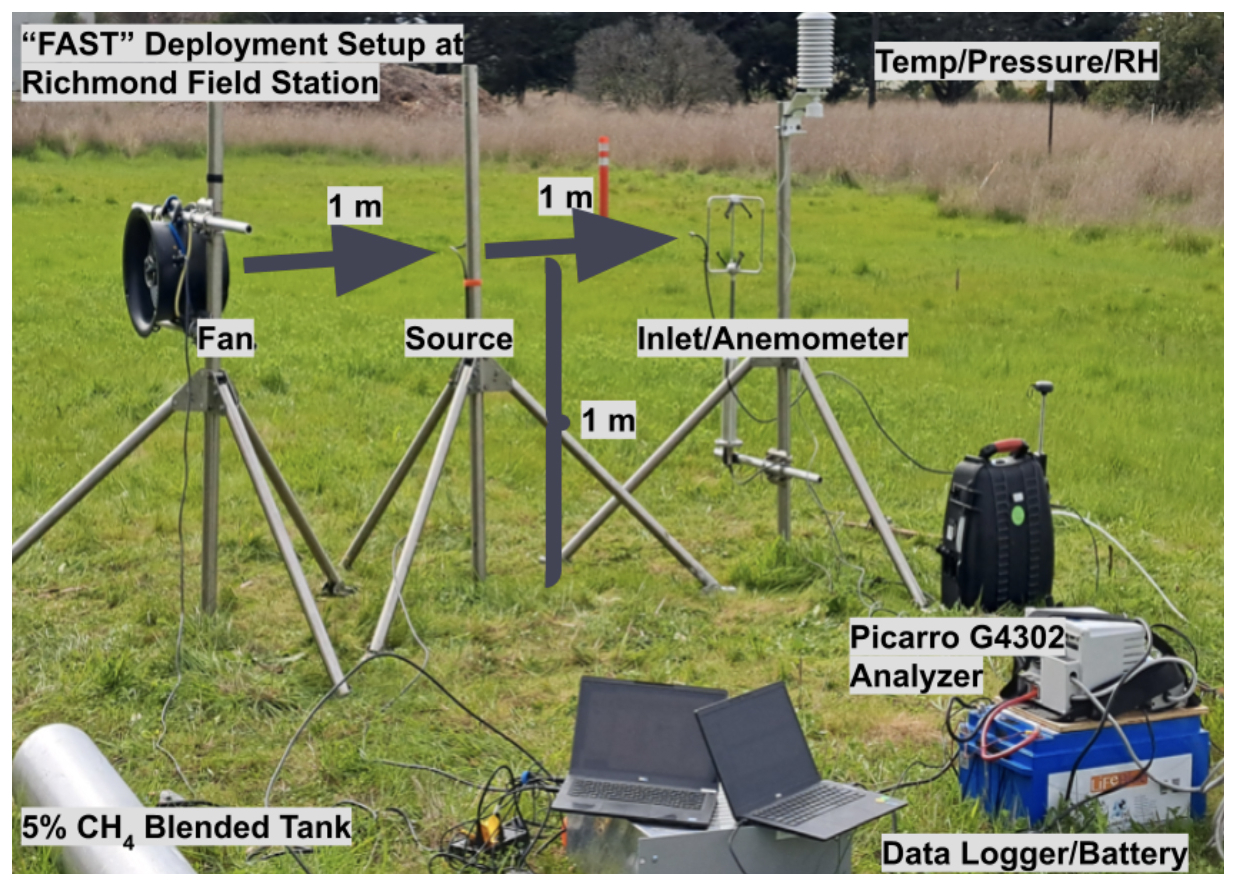
Figure 3 Experimental setup for the controlled-release experiment at Richmond Field Station in Richmond, CA. The MDB fan, the inlet for the Picarro G4302 analyzer and the Gill Windmaster 3D sonic anemometer were mounted at 1 m height at a distance of 2 m from one another (upper limit for the FAST method). A source of 5 % methane blended with pure nitrogen was also mounted on a second tripod at a downwind distance of 1 m from the fan and outfitted with a piece of foam to ensure diffuse emissions.

Table 2 Equipment used during the controlled-release experiment at Richmond Field Station.

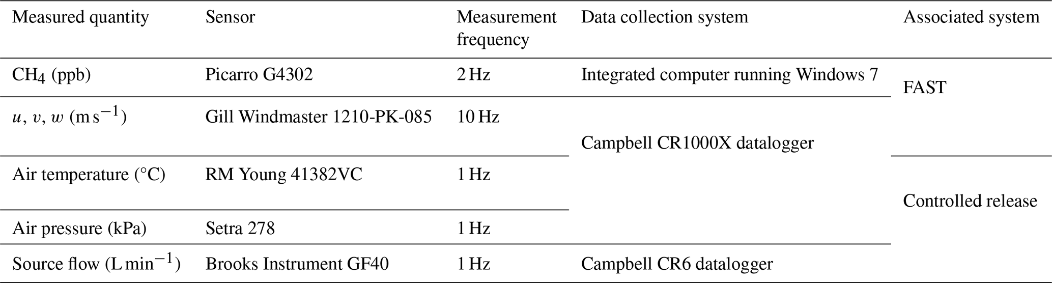
Sensor signals from wind, ambient air temperature, pressure and source output flow were collected using data loggers, with all data collection system clocks synchronized to within 1 s of UTC. The experiment began at 18:30 UTC with setup and preparation. At 20:19 UTC, the initial experiment for background (1.99 ± 0.36 ppm) measurements started with no source emission. The experiment involved different flow rates with corresponding durations. For each flow rate interval, the SEMTECH measurements were conducted in 2 min with no fan, followed by the FAST data collection for 10 min without the fan, 10 min with the fan at low intensity and 5 min of the fan at high intensity, with 5 to 10 min of adjustment between flow rate steps to avoid transient periods. The experiment concluded at 00:21 UTC (the following day).

2.2.2 Stoichiometry

The methane source leak rates (in g h⁻¹) are calculated using measured quantities of source flow, ambient air temperature, pressure and assumed constant source concentration. The measured quantities reported for each step were averaged over each measurement. The source leak rate Q is described in terms of measured quantities and known constants.

$$\begin{array}{}\text{(5)}& Q=C\mathit{\rho }\mathit{\kappa },\end{array}$$

where C is the CH₄ concentration from the source tank at 0.05 ± 0.0017 mol CH₄ per mol air, ρ is the CH₄ mass density (g L⁻¹) at measured ambient temperature and pressure, and κ is the corrected output mass flow of the source gas.

The CH₄ mass density is calculated in terms of measured qualities of ambient air pressure P and temperature T as

$$\mathit{\rho }=\left(M_{{\mathrm{CH}}_{\mathrm{4}}}/R\right)(P/T),$$

where $M_{{\mathrm{CH}}_{\mathrm{4}}}$ is molar mass 0.01604 kg mol⁻¹ of CH₄, and R is the universal gas constant 8.31446 (L kPa) (K mol)⁻¹. The corrected output mass flow κ is calculated from the measured flow rate κ_std reported at a standard temperature T_std of 293 K and measured ambient temperature T as

$$\mathit{\kappa }={\mathit{\kappa }}_{\mathrm{std}}(T/T_{\mathrm{std}}).$$

Rewriting Q in terms of measured quantities we find

$$\begin{array}{}\text{(6)}& Q=\mathit{\alpha }CP{\mathit{\kappa }}_{\mathrm{std}},\end{array}$$

where

$$\mathit{\alpha }=\left[M_{{\mathrm{CH}}_{\mathrm{4}}}/\left(R{T}_{\mathrm{std}}\right)\right].$$

The source leak rate uncertainty σ_Q (shown as error bars on Q estimates) is estimated from uncertainties in source concentration C, measured quantities of ambient air pressure P and output flow κ_std:

$$\begin{array}{}\text{(7)}& {\mathit{\sigma }}_Q=\mathit{\alpha }\sqrt{{\left(P{\mathit{\kappa }}_{\mathrm{std}}{\mathit{\sigma }}_C\right)}^{\mathrm{2}}+{\left(C\mathit{\kappa }{\mathit{\sigma }}_P\right)}^{\mathrm{2}}+{\left(CP{\mathit{\sigma }}_{\mathit{\kappa }}\right)}^{\mathrm{2}}},\end{array}$$

where the uncertainties σ_P and σ_κ are standard deviations of averaged data from the measurement windows. The time series of flow rates and measured atmospheric pressure during the course of the experiment are shown in Fig. 4.

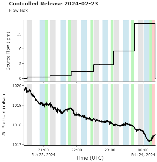
Figure 4 Time series of the output flow rate (liters per minute) throughout the Richmond controlled-release experiment with shaded areas indicating the set measurement windows: gray for no fan state, blue for fan on at low speed, green for fan on at high speed and red for maximum fan speed at the end of the experiment.

Similarly, the uncertainty in the flow rate estimated by the FAST method can be written as

$$\begin{array}{}\text{(8)}& \begin{array}{rl}& {\mathit{\sigma }}_{\widehat{Q}}=\\ & \sqrt{{\left(K_{\mathrm{FAST}}\underset{\mathrm{¯}}{C_{\mathrm{CL}}}{\mathit{\sigma }}_{\underset{\mathrm{¯}}{u_{\mathrm{CL}}}}\right)}^{\mathrm{2}}+{\left(K_{\mathrm{FAST}}\underset{\mathrm{¯}}{u_{\mathrm{CL}}}{\mathit{\sigma }}_{\underset{\mathrm{¯}}{C_{\mathrm{CL}}}}\right)}^{\mathrm{2}}+{\left(\underset{\mathrm{¯}}{C_{\mathrm{CL}}}\underset{\mathrm{¯}}{u_{\mathrm{CL}}}{\mathit{\sigma }}_{K_{\mathrm{FAST}}}\right)}^{\mathrm{2}}},\end{array}\end{array}$$

where ${\mathit{\sigma }}_{\underset{\mathrm{¯}}{u_{\mathrm{CL}}}}$ is the standard deviation of the wind speed in the downwind direction, ${\mathit{\sigma }}_{\underset{\mathrm{¯}}{C_{\mathrm{CL}}}}$ is the standard deviation of the concentration measurements and ${\mathit{\sigma }}_{K_{\mathrm{FAST}}}$ is the standard error in the estimate of K_FAST as shown in Fig. 7 and Table 4.

2.2.3 Data filtering by wind direction

In order to optimize the FAST method under strong crosswind conditions, filtering was applied to improve data quality and estimate emissions more accurately. Despite the advection from the fan, strong crosswind interference introduces variability in both the concentration (C) and wind speed (u) measurements. Filtering addressed this issue by excluding data associated with wind directions unlikely to transport emissions directly to the sensors.

To filter the data, we first calculate the wind direction (Θ_i) from the x- and y-direction wind components (u and v) within a normalized range of [0,360) ° for each data point as follows:

$$\begin{array}{}\text{(9)}& {\mathrm{\Theta }}_i=\left(\left(\text{arctan}\mathrm{2}(v,u)\times {\displaystyle \frac{\mathrm{180}}{\mathit{\pi }}}\right)+\mathrm{360}\right)\text{mod}\mathrm{360}.\end{array}$$

The mean wind direction, Θ_mean, is then computed as the arithmetic average of the normalized wind directions:

$$\begin{array}{}\text{(10)}& {\mathrm{\Theta }}_{\mathrm{mean}}={\displaystyle \frac{\mathrm{1}}{N}}{\sum }_{i=\mathrm{1}}^N{\mathrm{\Theta }}_i,\end{array}$$

where N represents the total number of data points in a given measurement period.

We then apply a filter angle (ϕ) symmetrically around the mean wind direction to define the range of included data. The lower (Θ_lower) and upper (Θ_upper) bounds of the filtered range are defined as

$$\begin{array}{}\text{(11)}& {\displaystyle }{\mathrm{\Theta }}_{\mathrm{lower}}=\left({\mathrm{\Theta }}_{\mathrm{mean}}-{\displaystyle \frac{\mathrm{360}-\mathit{\varphi }}{\mathrm{2}}}\right)\text{mod}\mathrm{360},\text{(12)}& {\displaystyle }{\mathrm{\Theta }}_{\mathrm{upper}}=\left({\mathrm{\Theta }}_{\mathrm{mean}}+{\displaystyle \frac{\mathrm{360}-\mathit{\varphi }}{\mathrm{2}}}\right)\text{mod}\mathrm{360}.\end{array}$$

The wind and methane data are then filtered to include only directions within the specified range. If the bounds do not cross the 0°/360° discontinuity, the filtered data satisfy

$$\begin{array}{}\text{(13)}& {\mathrm{\Theta }}_i>{\mathrm{\Theta }}_{\mathrm{lower}}\text{and}{\mathrm{\Theta }}_i<{\mathrm{\Theta }}_{\mathrm{upper}},\end{array}$$

and when the bounds span the discontinuity, data satisfying the following conditions are used:

$$\begin{array}{}\text{(14)}& {\mathrm{\Theta }}_i>{\mathrm{\Theta }}_{\mathrm{lower}}\text{or}{\mathrm{\Theta }}_i<{\mathrm{\Theta }}_{\mathrm{upper}}.\end{array}$$

Figure 5 illustrates the impact of filtering on the time series of wind and methane concentration data, for a 1 g h⁻¹ release from the Richmond Field Station experiment (N = 300). As the filter angle decreases, more data from crosswind and background noise are excluded (shown in red) and the mean wind speed (u) and concentration (C) values change, resulting in different estimates from the FAST method. We found that a filter angle of 300° effectively aligns the analysis with wind directions closely aligned with the source when accounting for plume spread within x < 2 m.

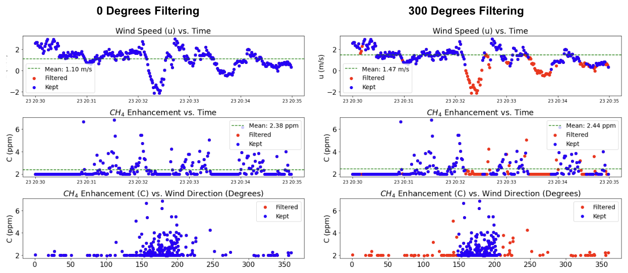
Figure 5 Time series of wind speed (u) and methane enhancement (C) as well as C vs. wind direction (in degrees) for a “no fan” release of 1 g h⁻¹ at the Richmond Field Station. Kept data are shown in blue, while filtered data are shown in red. Mean wind speed and concentration over the 5 min measurement period are shown in green.

2.3 Field experiments

The FAST method was tested on four wells during two field campaigns, two in Texas (6 and 7 February) and two in Oklahoma (14 March), during the spring of 2024. For all field measurements, a similar setup was used to that in the Richmond Field Station controlled-release experiment. During the experiments in Texas, the background wind velocity was < 1 m s⁻¹, so only the low fan setting was used for the two wells. In Oklahoma, background wind speeds were much higher than those in Richmond, so both the low fan and high fan settings were used. At each well, we measured background (upwind) methane concentrations using the Picarro for 5 min, and this background value was subtracted from the methane concentrations collected during the FAST method to determine the enhancement. Figure 6 shows images of the four wells discussed in the paper with the FAST method setup. For each well, SEMTECH and FAST measurements were taken; FLIR measurements were taken in Texas only.

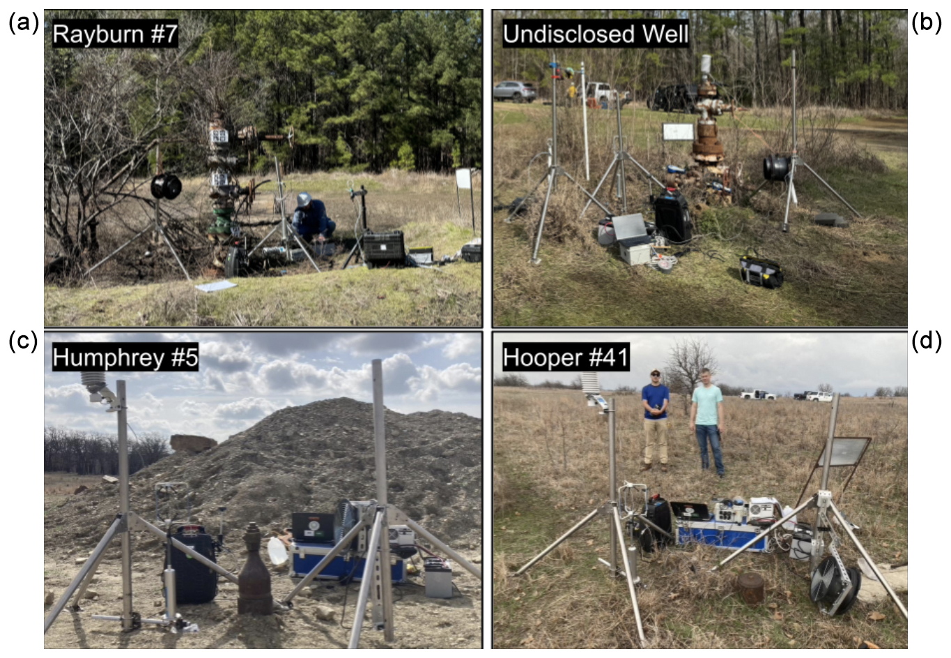
Figure 6 Wells measured in Lufkin, Texas (a, b), and Barnsdall, Oklahoma (c, d), using the FAST method. Both wells in Texas were of the “Christmas tree” variety (multiple potential leak points) and were measured using no fan and low fan speeds because the background wind speeds were < 1 m s⁻¹. Both wells in Oklahoma were lower to the ground; had only one leak point; and were measured with no fan, low fan and high fan speeds due to the higher background winds (> 1 m s⁻¹).

3 Results

3.1 Fan characterization results

Detailed results of the fan characterization experiments are provided in Appendix C. These experiments demonstrated that the high fan setting produced a more stable and uniform plume under higher background wind conditions, while the low setting was sufficient for generating a stable plume in the absence of background wind. Wind speed measurements showed that the primary flow velocity decreased with downwind distance, reaching background levels beyond approximately 2 m. The analysis of the standard deviation of wind direction confirmed that plume dispersion followed a square-root dependence on distance for x < 2 m, in agreement with theoretical expectations. Beyond this range, crosswind turbulence caused significant deviations from the expected dispersion behavior, leading to increased variability and instability in the plume structure. Additionally, measurements taken off the plume centerline (y ≠ 0) exhibited greater variability due to crosswind effects, reinforcing the importance of positioning sensors along the centerline (y = 0) to ensure consistent and reproducible measurements. Based on these findings, all field experiments were conducted with sensors placed within 2 m of the fan and along the centerline.

Furthermore, based on our fan experiments, we were able to estimate the parameters needed to calculate K_FAST using Eq. (4). We measured the blade length of the MDB fan (l_fan) and estimated the turbulence intensity i_fan as the mean of the turbulence intensity measured in the first fan experiment during the high and low fan settings for x < 2 m (see Figs. C1 and C2). Using these values (β = 1, i_fan = 0.23, l_fan = 0.13 m, x₀ = 2 m), the effective K_FAST would be K_FAST = πβ i_fanl_fanx₀ = 0.19 m², which matches the value determined during the controlled-release experiment with maximum filtering (300°).

3.2 Experimental determination of K_FAST

Results from the Richmond Field Station controlled-release experiment are summarized in Table 3. Using Eqs. (7) and (8), an estimate of the actual source rate (Q) was obtained which nearly matched the intended target rates of 1, 2, 5, 10, 20 and 40 g h⁻¹. The SEMTECH HI-FLOW performed very well during the controlled-release study, almost matching the exact values derived from stoichiometry. The FAST method estimates (generated using 10 min averages and K_FAST = 0.19 m²) also match the source rate quite well, however with much larger uncertainties than the SEMTECH. Without the fan (no fan), the FAST method tends to overestimate the lower range (1–5 g h⁻¹) and severely underestimate the upper range (10–40 g h⁻¹). This is greatly improved via the use of the fan, with the low fan setting performing slightly better in the upper range and the high fan setting performing better in the lower range. These discrepancies could also be due to fluctuations in the background wind throughout the experiment which may have biased the results.

Table 3 Comparison of the desired (target) and true (stoichiometric) release rate with those measured by the SEMTECH and FAST method (with 300° of filtering) during the controlled-release experiment at Richmond Field Station.

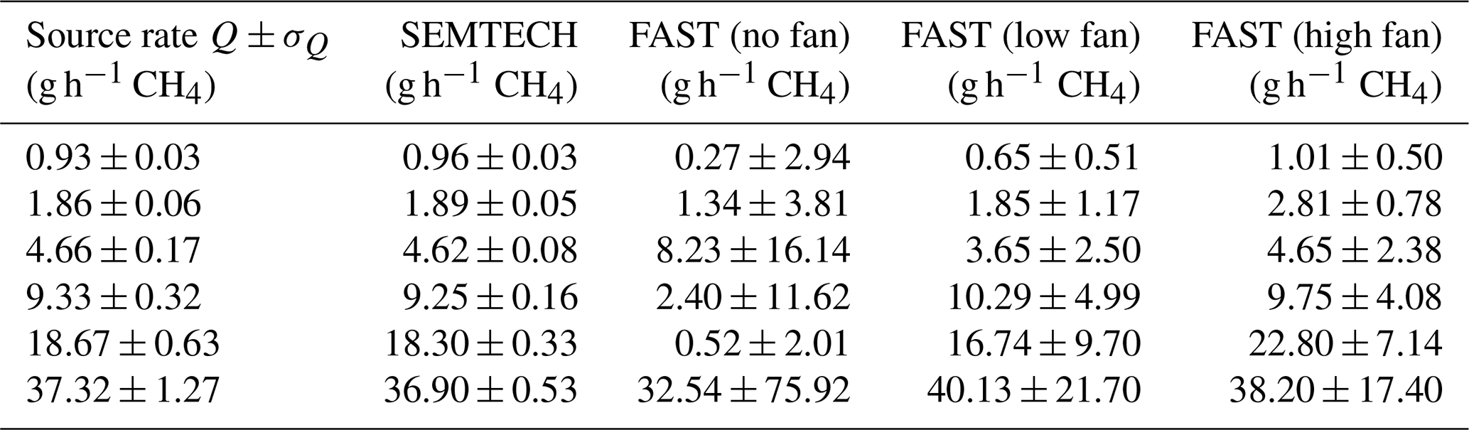
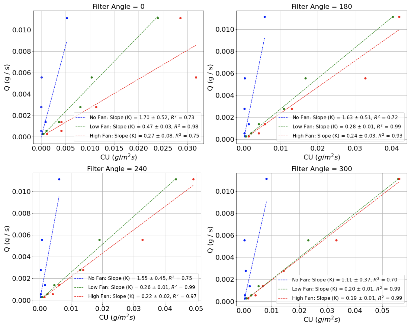
Figure 7 Measured mean C⋅U (along x) vs. known Q (along y) for the control release experiment used to determine the values of K_FAST (slopes) for a range of fan speeds and filtering angles.

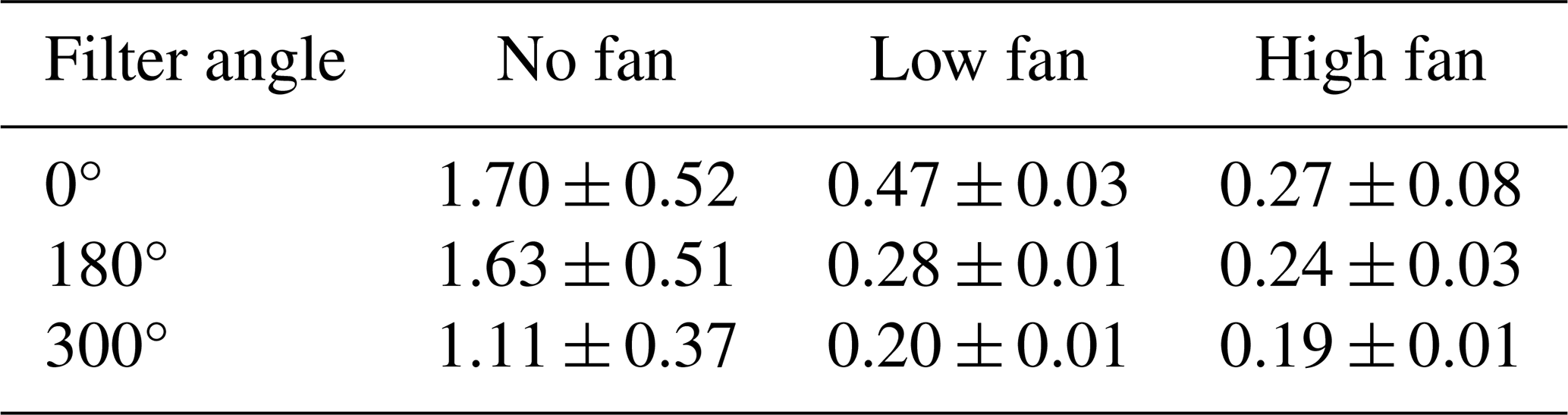
By using the known values of Q from stoichiometry (source rate) and the measured values of C and u during the controlled-release experiment, the experimentally determined values of K_FAST for different filter angles and fan speeds are estimated via Eq. (3). By inverting Eq. (3) to solve for K_FAST, K_FAST = $\frac{\stackrel{\mathrm{‾}}{C_{\mathrm{CL}}}\stackrel{\mathrm{‾}}{u_{\mathrm{CL}}}}{Q}$, where the known value of Q and 10 min averages of C_CL and u_CL are used to estimate K_FAST. The resulting values for K_FAST are shown as the slopes of the lines in Fig. 7 along with the uncertainties resulting from standard error estimates on the linear regression used to generate the line of best fit. As expected, the no fan scenario has a much higher value of K_FAST with higher overall uncertainty due to the variation in the natural wind direction and speed. Without filtering the data by wind direction, the K_FAST values are larger (likely due to more dispersion from crosswinds). Furthermore, K_FAST values at the low and high fan speeds do not agree, although K_FAST is theoretically independent of fan speed (per Eq. 4). As more and more crosswind is filtered (filter angle approaches 360°), the low and high fan speeds converge to a K_FAST of around 0.19 m², as expected. All fits are done with a 0 intercept, and standard errors are used to estimate the uncertainty in K_FAST. Table 4 shows the resulting experimentally determined values of K_FAST and their corresponding uncertainties which were used to estimate emissions and corresponding uncertainties from field measurements.

Table 4 Values of K_FAST (in m²) and their associated uncertainties under various filter and fan conditions determined from the Richmond controlled-release experiment.

3.3 Field campaigns

3.3.1 Texas field campaign

The first field campaign that measured orphaned wells using the FAST method took place in February 2024 in collaboration with multiple agencies. The U.S. Forest Service (USFS) invited the U.S. Department of Energy's Consortium Advancing Technology for Assessment of Lost Oil and Gas Wells (CATALOG) team to help measure and assess emissions from certain wells being plugged using funds from the Infrastructure Investment and Jobs Act (IIJA). The FAST method was deployed in the field campaign to understand emission patterns better and help allocate sealing funds more efficiently.

Rayburn #7

Rayburn #7 is an oil production well identified by API number 4200530245 and associated with district/lease number 06/13688. Its geographical coordinates are 31.0865, −94.1974, and its total depth is 12 927 ft (3940.1 m). On 6 February 2024 during the initial detection of Rayburn #7, a small leak was found from a threaded port on a valve junction 1.2 m above the ground by sniffing the casing of the well with the Picarro G4302. The well is situated in a large clearing with a gravel pad and other infrastructure surrounded by an embankment. A plastic spill tub and several 500 gallon (1893 L) drums were observed close to the wellhead. Furthermore, a compressor station and separation/storage infrastructure are located in the corner of the clearing. No leak was detected on any of the other infrastructure in the area. A Gill R3-50 sonic anemometer was placed at the height of 1.2 and 0.94 m away from the methane source alongside the inlet to the Picarro G4302 methane detector. Sampling commenced at 12:20 UTC under ambient conditions for 60 min. The background methane concentration was 2.11 ppm. Following this, there were two more sets of sampling periods: 30 min each for ambient conditions and low fan conditions. The SEMTECH measured an emission rate of 2.86 g h⁻¹, with a standard deviation during the averaging period of ±0.04 g h⁻¹ (Fig. B2a). The FLIR camera could not provide a clear visual indication of the leak.

Figure 8 illustrates the effect of using the fan on the time series of concentration and wind speed measurements at Rayburn #7, providing insight into the variability in methane concentrations and plume enhancements. Without the fan (Fig. 8, left), the average wind speed in the x direction (u) over the 30 min measuring period was approximately 0 m s⁻¹. However, infrequent gusts in the x direction caused spikes in methane concentrations, ranging from about 10 to 20 ppm above background levels. These spikes were spread across a wide range of directions, between 100 and 250°, indicating variable plume dispersion under stagnant conditions. With the fan on at a low setting (Fig. 8, right), the mean wind speed in the x direction (u) increased to approximately 2 m s⁻¹, and the plume became more stable. The methane concentration spikes were more concentrated in direction, between 180 and 210°, corresponding to the airflow from the fan. While a large spike was observed at the start of the low fan measurement, likely due to the fan turning on, the concentration stabilized to around 5 ppm above background levels after this initial adjustment.

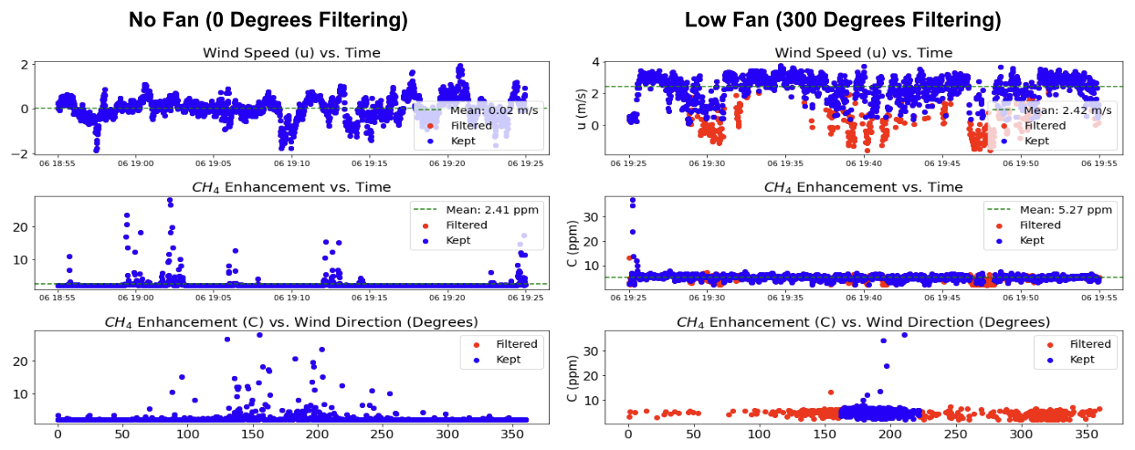
Figure 8 Time series of wind speed (u) and methane enhancement (C) as well as C vs. wind direction (in degrees) for “no fan” setting from a “low fan” setting. Kept data are shown in blue, while filtered data are shown in red. Mean wind speed and concentration over the 30 min measurement periods are shown in green.

Undisclosed well

The methane emission detection and monitoring experiment at this undisclosed location identified two leak points on one wellhead. The FLIR did not detect any emissions from either of the leak sources. There was a small leak at the end of a main pipe flange and a more significant leak in a connection thread on the same flange, which was the primary point source. The FAST system was set up at 11:45 UTC on 7 February 2024, pointed at 315° N, with the fan turned off. The fan was located 58 cm above the ground and 87 cm upwind of the source, which is within the range of < 1 m. The Gill R3-50 sonic anemometer and Picarro G4302 gas analyzer inlets were positioned 73 and 71 cm above the ground and 97 and 95 cm horizontally from the source, respectively. The primary source was at a height of 47 cm. The background methane concentration was 2.08 ppm. The experiment with the fan turned on started at 13:22 UTC. Data were collected for two 15 min periods with the fan on and two 15 min periods with the fan off. Analogous to the Rayburn #7 experiment, the anemometer orientation was set in a manner that 0° represents the direction where it is facing the upwind source and fan line. For this experiment, wind direction had favorable conditions, which led to significant data acquisition for the periods without the fan. The SEMTECH measured an emission rate of 0.95 g h⁻¹, with a standard deviation during the averaging period of ±0.25 g h⁻¹ (Fig. B2b).

3.3.2 Oklahoma field campaign

Humphrey #5

Humphrey #5 is an orphaned well that was located by our team during surveying on 14 March 2024. The FAST method was set up and measured for 10 min at each fan speed (no, low, high) as shown in Fig. 9. The leak was from the top cap of the well head at a height of 0.62 m, and the sensors were positioned downwind at 0.4 m from the leak and a height of 0.65 m. The fan was set up at a height of 0.6 m and an angle of 5° upward (to generate a plume that passed through the anemometer) at 0.5 m upwind of the well. The SEMTECH measured an emission rate of 2.03 g h⁻¹, with a standard deviation during the averaging period of ±0.04 g h⁻¹ (Fig. B2c).

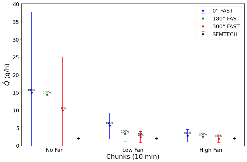
Figure 9 Estimated leak rates ($\widehat{Q}$) and uncertainties (${\mathit{\sigma }}_{\widehat{Q}}$) from the FAST method measured in 10 min increments (colored) and SEMTECH (black) for Humphrey #5, labeled by percentage of data kept after filtering. For the “no fan” setting (left most), the estimate is very uncertain and much higher than the SEMTECH.

Hooper #41

Hooper #41 is another undocumented orphaned well (UOW) that was also discovered by the team on 14 March 2024 near Barnsdall, OK. The leak was from the top cap of the well head at a height of 0.25 m, and the sensors were positioned downwind at 0.88 m from the leak and a height of 0.65 m. The fan was set up at a height of 0.27 m and an angle of 24° upward at 0.4 m upwind of the well. Interestingly, this well seemed to have a variable leak rate, resulting in a very high uncertainty on the SEMTECH. The SEMTECH measured an intermittent averaged emission rate of 70.14 g h⁻¹, with a large standard deviation during the averaging period of ±95.47 g h⁻¹ (Fig. B2d). The FAST method was used in 10 min intervals for no, low and high fan settings. Due to the highly variable nature of the well, these measurements were repeated in the same intervals for comparison (Fig. 10). During both measurement periods, the FAST method estimates the well to only emit around 10 ± 10 g h⁻¹ as opposed to 70 ± 90 g h⁻¹, which the SEMTECH reported.

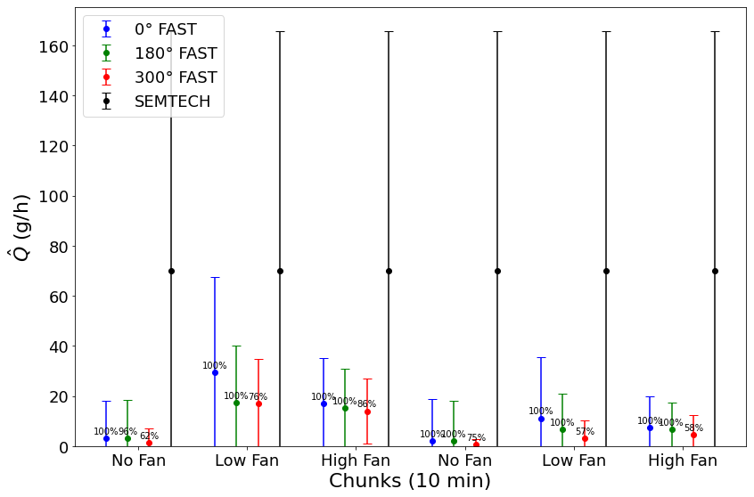
Figure 10 Estimated leak rates ($\widehat{Q}$) and uncertainties (${\mathit{\sigma }}_{\widehat{Q}}$) from the FAST method measured in 10 min increments (colored) and SEMTECH (black) for Hooper #41, labeled by percentage of data kept after filtering. Due to the high variability in the well, it was measured twice with the FAST method at 10 min increments (sequentially). Here, the SEMTECH did not get a good reading due to the instability in the CH₄ concentration of the sampling volume.

The results for Hooper #41 highlight challenges in measuring methane emissions from variable wells and suggest potential limitations in the FAST method. The variable leak rate led to significant uncertainty in SEMTECH readings (±95.47 g h⁻¹), while the FAST method provided more stable estimates (10 ± 10 g h⁻¹). However, the fan setup likely failed to fully entrain the emitted gas into the airflow directed toward the sensor, potentially leading to an underestimation of emissions, as supported by SEMTECH data and Fig. 10. This limitation is particularly critical for wells with low-height emissions, such as Hooper #41. Future work could address this limitation through controlled-release experiments at different heights to optimize the fan and sensor configurations for capturing low-lying plumes.

4 Discussion

The results of the field campaigns are summarized in Table 5 and Fig. 11. For each of the four wells measured, the FAST method results are based on 10 min averages and K_FAST values corresponding to the fan speed and various levels of filtering (0, 180 and 300°) as shown in Fig. 7 and Table 4. The uncertainty in the FAST estimates is calculated using Eq. (8). Overall, the FAST method agrees with the SEMTECH for both the low and high fan settings but not for the no fan settings. These uncertainties decrease with a larger filtering angle and a higher fan speed. Furthermore, emission rate estimates for all four wells were calculated using a Gaussian plume model (GPM) and are described in Appendix A for comparison.

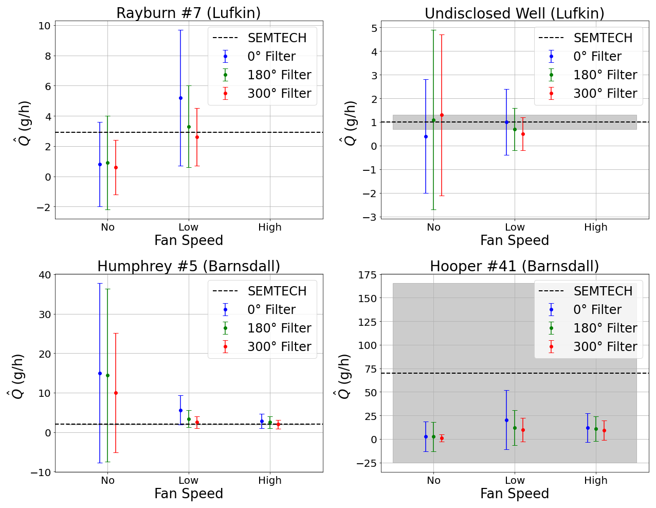
Figure 11 Estimated leak rates ($\widehat{Q}$) and uncertainties (${\mathit{\sigma }}_{\widehat{Q}}$) for the four wells shown in Fig. 6 from the SEMTECH (black and gray) and FAST method (colored). SEMTECH is able to get very accurate readings for all wells except Hooper #41, which was a highly variable well.

Table 5 Estimated leak rates ($\widehat{Q}$) and uncertainties (${\mathit{\sigma }}_{\widehat{Q}}$) for the four wells shown in Fig. 6 from the SEMTECH and FAST method. SEMTECH is able to get very accurate readings for all wells except Hooper #41, which was a highly variable well.

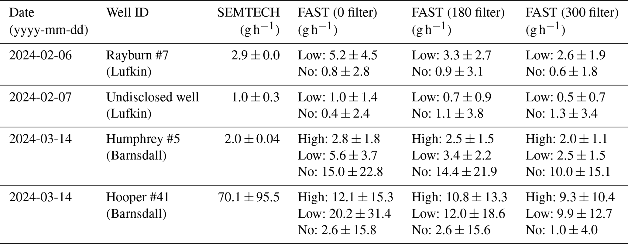
Figure 12 shows the results of the FAST method at the low fan (blue) and no fan (red) settings on Rayburn #7, which was measured in 30 min intervals, as well as the SEMTECH estimate (dashed black line). For the low fan setting, the SEMTECH value is always within the uncertainty of the FAST method, even if only the first minute of data is used. The mean rate improves when the measuring time is increased to 3 min, but the error bars remain large. For measuring times larger than 3 min, the error bars decrease nearly linearly with increased measuring time, while the mean stays relatively constant. The no fan results, on the other hand, do not match the SEMTECH well for measuring times shorter than 10 min. As expected, as the measuring time increases, the mean value of the FAST method for no fan gradually approaches the SEMTECH, but the error bars also increase over time. This shows that the measuring time for the FAST method, even at the low fan measurement, is similar to that of the SEMTECH (on the order of 3 min).

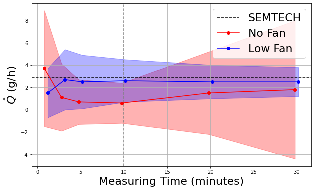
Figure 12 Estimated leak rates ($\widehat{Q}$) and uncertainties (${\mathit{\sigma }}_{\widehat{Q}}$) from the FAST method for Rayburn #7 as a function of the sampling time used to make the estimate. Without a fan, the measurement is highly uncertain throughout, except for the range from 5–10 min. With the fan, the measurement accuracy gets higher with increasing measurement time, but the mean value stays roughly constant above 3 min. This shows that the FAST method can be done as quickly as the SEMTECH and accuracy only increases with increased measuring time.

The total cost of the sensors used in this study, a Picarro G4302 for concentration (∼ USD 40 000) and Gill Windmaster 1210-PK-085 (∼ USD 5000) for wind, is about the same cost as a SEMTECH HI-FlOW (∼ USD 50 000). However, the FAST method can be done without using 3D wind measurements. By replacing the 3D anemometer with a 1D anemometer, the cost of the FAST method can be decreased with minimal loss in accuracy. Effectively, using a 1D anemometer would limit the filter angle to be up to 180°, which has marginally worse accuracy than filtering by 300°. Furthermore, the type of methane sensor can be optimized to a more reasonable price point, as CH₄ signals near sources are typically high (e.g., > 1 ppm for leaks > 1 g h⁻¹). Future work will focus on investigating a wide variety of methane detection technologies to identify more cost-effective and reliable solutions for widescale FAST method deployment.

Besides its potential for being lower cost, the FAST method has other advantages over the existing technologies we tested (FLIR and SEMTECH). First, the FLIR camera is insensitive to small leaks and unable to detect most diffuse emissions and is unable to quantify emissions accurately (Zeng and Morris, 2019). Furthermore, while our existing proof-of-concept FAST hardware is currently heavier and more complex to operate than a SEMTECH, it could be replicated with a battery-powered fan mounted to a tripod or a backpack vacuum blower, making it very similar to the size and labor requirements of the SEMTECH. Although both the FAST method and the SEMTECH take approximately 3 min to obtain a measurement, the FAST method currently requires a longer setup time (∼ 30 min) compared to the SEMTECH (∼ 5 min).

5 Conclusions

We have shown that using a fan to create a forced flow at close range between the emission source and a point methane (CH₄) sensor and measuring 3D wind profiles using a sonic anemometer and CH₄ concentration with a gas analyzer (sampling technique), a simple estimate of the CH₄ emission rate of the source can be inferred (FAST method). The FAST method has been tuned using single, continuous point sources between 0.9 and 37 g h⁻¹ at 1 m above the ground in a simple aerodynamic landscape (grass field) in moderate meteorological conditions (< 5 m s⁻¹). Under these conditions, the FAST method consistently provided reasonable estimates of leak rates when fan speeds and filtering were applied appropriately, performing similarly to the commercially available method (SEMTECH) and outperforming others (FLIR). Notably, the method's performance improves with increased fan speed and filtering angle. For instance, in the case of Rayburn #7 in Lufkin, Texas, the FAST method at the low fan speed consistently produced leak rate estimates that were within the uncertainty bounds of the SEMTECH values after just a few minutes of measurement. Without the use of a fan, the results showed much greater uncertainty, highlighting the importance of airflow in stabilizing methane dispersion for accurate estimation.

In the Texas and Oklahoma field campaigns, the FAST method provided accurate and rapid readings under varying environmental conditions, with errors on the order of 95 % of the emission rate across different wind conditions and leak rates. In Texas, where wind speeds were low, only the low fan setting was used, and FAST results aligned closely with SEMTECH, within 10 %. In Oklahoma, higher wind conditions required both low and high fan settings to account for greater natural dispersion. At Hooper #41, where emission rates fluctuated significantly, FAST produced lower overall estimates than SEMTECH, likely due to its larger sampling cross-section averaging out short-term variability. However, fan-driven airflow may not fully entrain all emitted gas, particularly from low-height leaks, which could contribute to an underestimation of emission rates in certain cases.

The FAST method offers a potential alternative to existing technologies such as SEMTECH and FLIR for identifying high-priority orphan wells. Its combination of controlled airflow and real-time methane measurement enables rapid assessments suitable for large-scale monitoring. Ongoing research aims to refine wind and methane sensor integration to improve cost efficiency while maintaining measurement accuracy across diverse field conditions and leak rates.

Appendix A: Comparison to Gaussian plume method

The approach to deriving the equations governing the FAST method outlined in the “Mathematical model” section can also be compared to the more traditional approach using a Gaussian plume model (GPM). Through this comparison, we can gain deeper insight into the physical significance of the proportionality constant (β), as it relates to the diffusivity of the pollutant of interest. Including a term for reflection from the ground (but not from an inversion aloft), the GPM estimates the downwind concentration of a pollutant as a function of the emission rate (Q), advective velocity (u), crosswind distance from centerline (y), vertical displacement from centerline (z), height of the emission source (H), and horizontal and vertical dispersion coefficients (σ_yσ_z) as follows:

$$\begin{array}{}\text{(A1)}& \begin{array}{rl}C(x,y,z)=& {\displaystyle \frac{Q}{\mathrm{2}\mathit{\pi }{\mathit{\sigma }}_y{\mathit{\sigma }}_{z}u}}\exp {\displaystyle \frac{-y^{\mathrm{2}}}{\mathrm{2}{{\mathit{\sigma }}_y}^{\mathrm{2}}}}\\ & \left(\exp {\displaystyle \frac{-(z-H{)}^{\mathrm{2}}}{\mathrm{2}{{\mathit{\sigma }}_z}^{\mathrm{2}}}}+\exp {\displaystyle \frac{-(z+H{)}^{\mathrm{2}}}{\mathrm{2}{{\mathit{\sigma }}_z}^{\mathrm{2}}}}\right).\end{array}\end{array}$$

Similar to the FAST model, the GPM assumes that the velocity profile is constant in space. However, the GPM does not assume the concentration profile is constant, which is implicitly done by the FAST method via the use of centerline time-averaged concentrations (Fig. A1). Rather, the GPM assumes that the concentration profiles are Gaussian in the y and z directions, with standard deviations (σ_y, σ_z) related to the width of the plume. These standard deviations are often approximated using empirical data (i.e. Pasquill stability classes) but can be defined exactly using the diffusivity of the pollutant (D). Assuming that the plume is isotropic and homogeneous, we can define

$$\begin{array}{}\text{(A2)}& {\mathit{\sigma }}_y\approx {\mathit{\sigma }}_z\approx \widehat{\mathit{\sigma }}=\sqrt{{\displaystyle \frac{\mathrm{2}Dx}{u}}},\end{array}$$

where D is the diffusivity of the pollutant and $\widehat{\mathit{\sigma }}$ is the standard deviation of the Gaussian plume in all directions orthogonal to x. Evaluating this equation at some downwind distance x₀ and substituting our earlier use of centerline velocity measurements (given that the velocity profile is assumed constant in both GPM and FAST), we can define the standard deviation there (${\widehat{\mathit{\sigma }}}_{\mathrm{0}}$):

$$\begin{array}{}\text{(A3)}& {\widehat{\mathit{\sigma }}}_{\mathrm{0}}\approx \sqrt{{\displaystyle \frac{\mathrm{2}D{x}_{\mathrm{0}}}{\underset{\mathrm{¯}}{u_{\mathrm{CL}}}}}}.\end{array}$$

Using this standard deviation, we can imagine integrating the FAST approach over a certain number of standard deviations to capture more and more of the true concentration profile. To capture 99.7 % of the total plume, we would need to integrate out to 3 standard deviations, or 3${\widehat{\mathit{\sigma }}}_{\mathrm{0}}$. Using this comparison to the previous equation derived for FAST (Eq. 2), we can solve for β.

$$\begin{array}{}\text{(A4)}& \begin{array}{l}{\mathit{\sigma }}_{\mathrm{0}}=\sqrt{\mathit{\beta }{i}_{\mathrm{fan}}{l}_{\mathrm{fan}}{x}_{\mathrm{0}}}\simeq \mathrm{3}{\widehat{\mathit{\sigma }}}_{\mathrm{0}}\approx \mathrm{3}\sqrt{\frac{\mathrm{2}D{x}_{\mathrm{0}}}{\underset{\mathrm{¯}}{u_{\mathrm{CL}}}}}\\ \mathit{\beta }\approx \frac{\mathrm{18}D}{i_{\mathrm{fan}}{l}_{\mathrm{fan}}\underset{\mathrm{¯}}{u_{\mathrm{CL}}}}\end{array}\end{array}$$

Here, we find that the proportionality constant β can be understood as a non-dimensional ratio of two diffusivities – one being the true diffusivity of the gas and the other being due to the turbulence generated by the fan. Since D can be very difficult to measure, the FAST method provides a work-around such that only constants related to the fan-generated flow need to be defined to quantify the emission rate. Equation (A5) could also be inverted to estimate the diffusivity D, but this is not of real interest for this study.

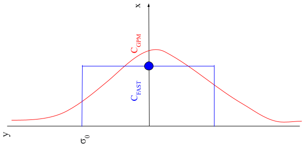
Figure A1 Diagram showing the difference in concentration profiles (C) used by the FAST (blue) and GPM (red) methods.

We also calculated the estimated emissions from a Gaussian plume model (GPM) using three different Pasquill stability classes (A, B and C) based on the no fan concentration and wind measurements for each well (shown in Table A1). As evidenced by the order of magnitude range for each well, the GPM is highly sensitive to the choice of stability class, which is not immediately apparent for such short-range measurements. We used the equations for calculating σ_y and σ_z from Cooper and Alley (2011, pp. 662–663).

Based on there being moderate to strong insolation and low wind speeds (< 2 m s⁻¹) for the Texas wells, the most likely stability class for Rayburn #7 and the undisclosed well is Class A or B. Using these stability classes, the GPM does reasonably well at estimating the magnitude of the leak, but the uncertainty is much higher than both the SEMTECH and the FAST methods. Due to the higher background wind speeds (3–5 m s⁻¹) and moderate to strong insolation in Oklahoma, the B and C stability classes are most likely for Humphrey #5 and Hooper #41. Here, the GPM overestimates the magnitude of Humphrey #5 by orders of magnitude and the uncertainty is very high. For Hooper #41, which is a highly variable well, the GPM also still performs poorly relative to the SEMTECH and FAST methods.

Table A1 Estimated leak rates ($\widehat{Q}$) and uncertainties (${\mathit{\sigma }}_{\widehat{Q}}$) for the four wells shown in Fig. 6 from the SEMTECH, FAST method (filtered) and a Gaussian plume model (GPM) for all possible daytime Pasquill stability classes.

Appendix B: SEMTECH measurements

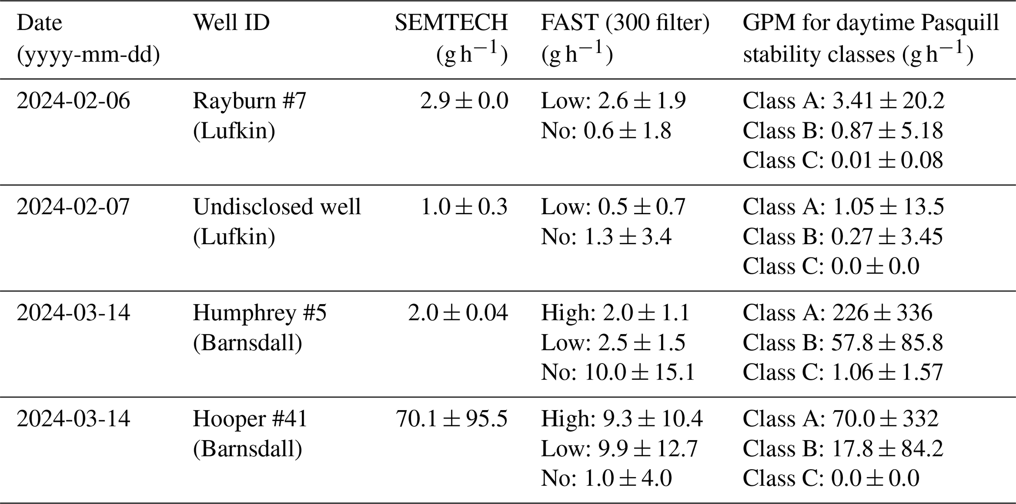
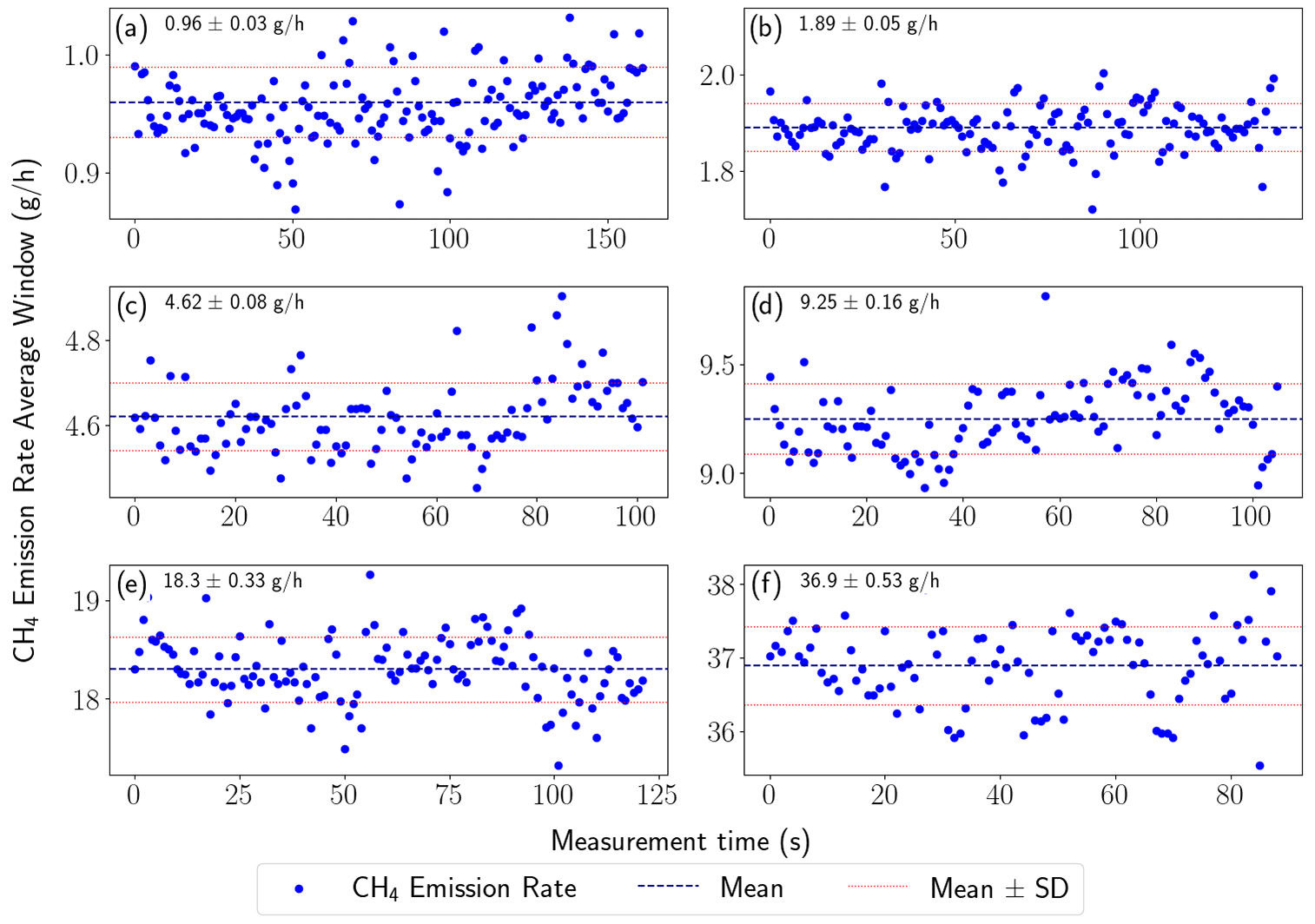
Figure B1 From left to right and top to bottom, the panels show the increasing step measurements of controlled-release emission rates from the SEMTECH. As the control release flow rate increases, the accuracy and precision of the SEMTECH decrease.

The SEMTECH Hi-Flow 2 is a methane emission quantification system composed of a backpack-mounted gas analyzer and a long sampling inlet tube with a fan to sample the methane emitted by a point source. This system reports the flow of methane emitted in liters per minute (L min⁻¹) in a range of 0.02 to 730 L min⁻¹ (1 g h⁻¹–29 kg h⁻¹) (0.001 to ∼ 25 ft³ min⁻¹ (1 ft³ min${}^{-\mathrm{1}}=$ ∼0.028 m³ min⁻¹), with an accuracy of ∼ 10 % (SEMTECH, 2024).

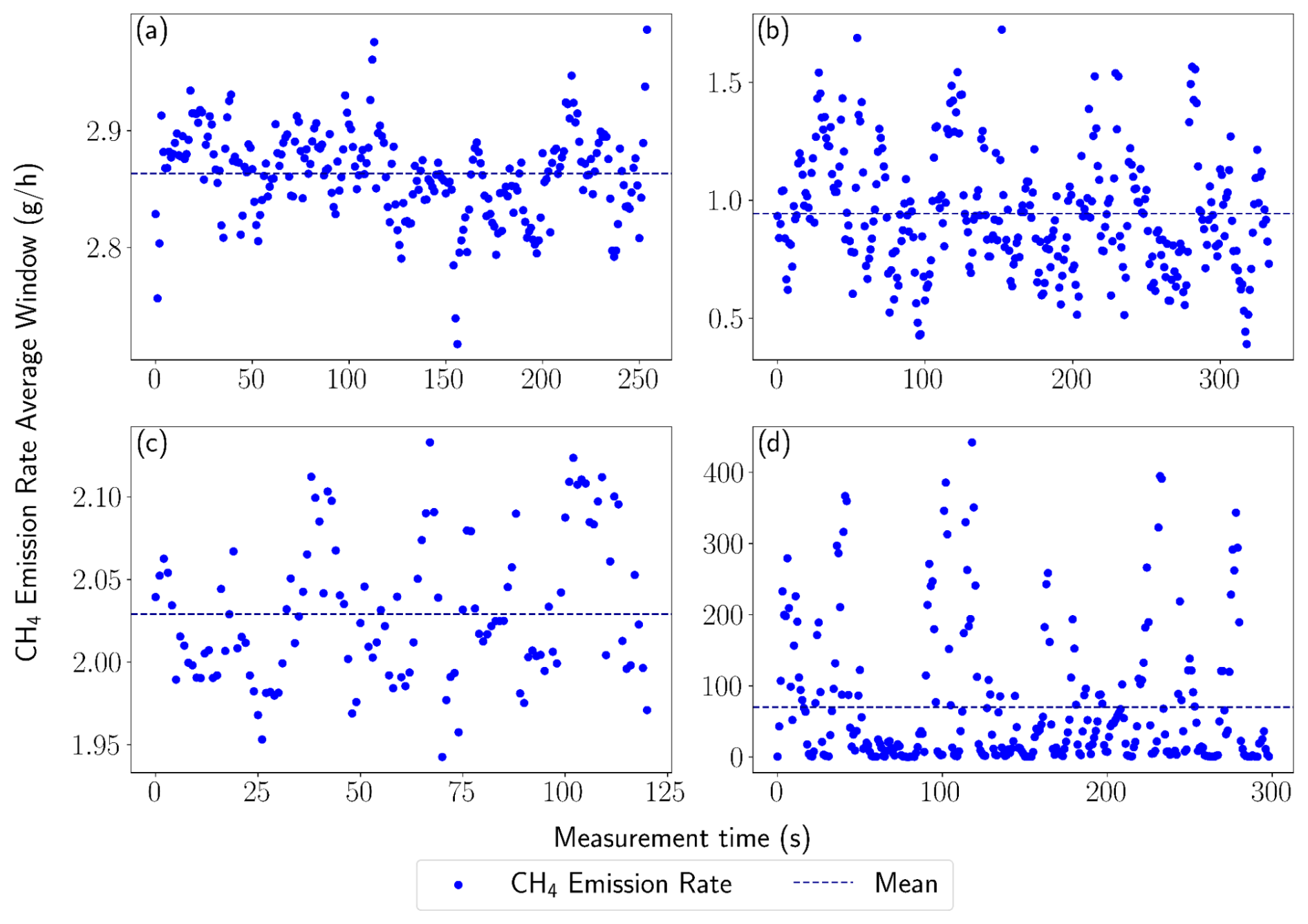
Figure B2 SEMTECH HI-FLOW measurements (time series and mean) from the four orphaned wells used in the FAST method validation.

The measurement principle of the SEMTECH HI-FLOW relies on simultaneous measurements of air flow and methane concentration. If F_air is the volumetric flow rate of air captured by the system (in L min⁻¹), C is the concentration of methane in parts per million; C_background is the concentration of methane of the background; and $K(T,P,\mathit{\eta })$ is an adjustment parameter varying with temperature (T), pressure (P) and air viscosity (η), then we can express the volumetric flow rate of methane $F_{{\mathrm{CH}}_{\mathrm{4}}}$ as

$$\begin{array}{}\text{(B1)}& F_{{\mathrm{CH}}_{\mathrm{4}}}=F_{\mathrm{air}}\cdot \left(C-C_{\mathrm{background}}\right)\cdot K(T,P,\mathit{\eta }).\end{array}$$

The velocity of the air is measured using a pitot tube, and the concentration of methane is measured using a gas analyzer (near-IR laser absorption CH₄ sensor sensitive to a range of 10 ppm to 100 % of CH₄) located in the backpack. All other parameters such as temperature and pressure are also measured by the SEMTECH directly in the pitot tube. This system is designed to be user-friendly, as the flow measured is directly shown on the system monitor. Data are logged every second (1 Hz). For example as we can see in Figs. B1 and B2, the SEMTECH measures the CH₄ emission rate, at a rate of one point per second, and returns a value in liters per minute (L min⁻¹) which we converted to grams per hour (g h⁻¹) for more convenient use.

Appendix C: Fan characterization results

The results of the first fan characterization experiment are summarized in Figs. C1–C3. Figures C1 and C2 show the mean wind speed in 3D (u, v, w), standard deviation of wind direction in the x–y (SD(wd_y)) and x–z (SD(wd_z)) planes, and turbulence intensity in the y (i_y) and z (i_z) directions in the range of downwind distances (x) for the low and high fan speeds, respectively. For both fan speeds, the u component of the flow starts higher than the background and decreases nearly linearly with distance until it is on the same order of magnitude as the background crosswind gust intensity (dashed blue line). The SD(wd_y) and SD(wd_z) values are calculated using the Yamartino method (Bruce Turner, 1986) and act as an estimate of the effective width of the plume (in radians). According to Eq. (2), these should both therefore grow proportional to x^0.5, which is verified for x < 2 m in Fig. C3. The turbulence intensities (i_y) and (i_z) are calculated using the means of the magnitudes of u, v and w as mean(v) $/$ mean(u) and mean(w) $/$ mean(u), respectively. These should be relatively constant for the fan-generated flow (i_fan) and about equal if the turbulence of the flow is uniform. The uniform flow near the fan is much more evident in the high fan data (Fig. C2), whereas the low fan measurements (Fig. C1) indicate the effects of crosswind turbulence, resulting in much larger values of i_y compared to i_z. It is also important to note that during the measurement period for the high fan speed, the crosswinds far exceeded their background value, resulting in a total disruption of the plume in this region (2 m < x < 3 m). The crosswinds died down later in the experiment when the anemometer was further downwind, resulting in a more stable plume for x > 3 m. Overall, we found that the fan plume remained stable under a wide range of crosswind conditions in the range of 1 m < x < 2 m.

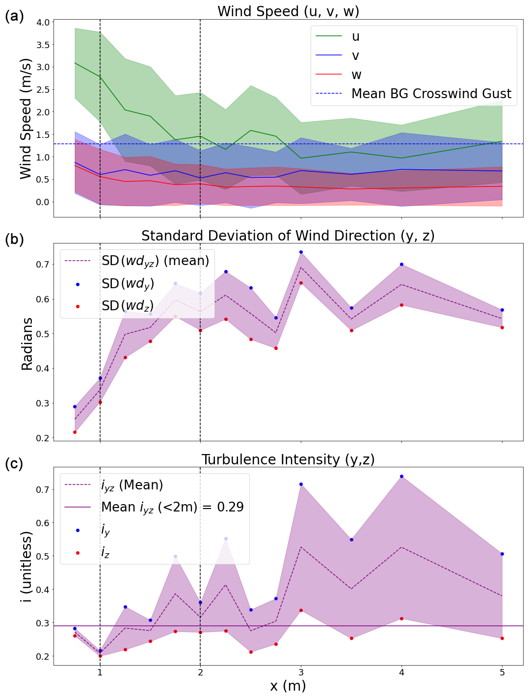
Figure C1 (a) Wind speed, (b) standard deviation of wind direction and (c) turbulence intensity as a function of downwind distance x for Experiment 1 using the low fan speed setting. Data are filtered to remove any points coming from the negative x direction (180°).

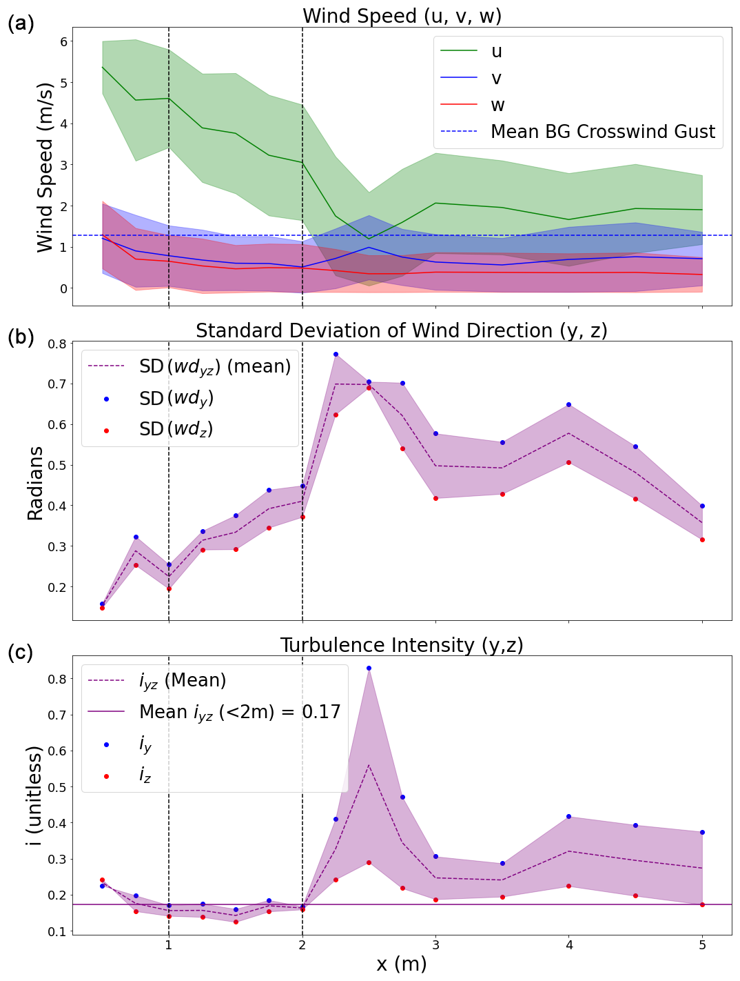
Figure C2 (a) Wind speed, (b) standard deviation of wind direction and (c) turbulence intensity of Experiment 1 using the high fan speed setting. Data are filtered to remove any points coming from the negative x direction (180°).

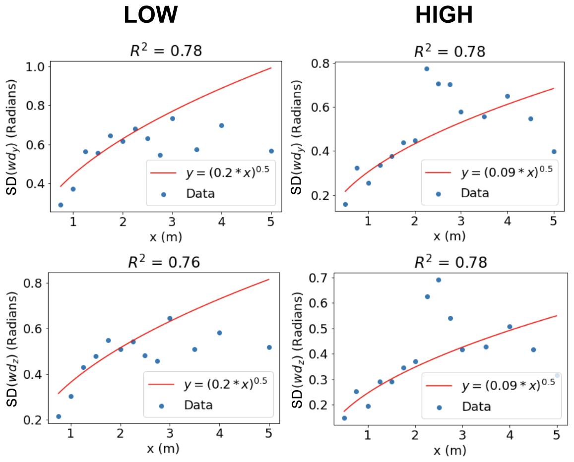
Figure C3 Square-root fits to the standard deviations (SDs) of wind direction with filter angle = 180° as expected from Eq. (2). The fits are valid in the range of 1–2 m and depart from the square-root curve at larger downwind distances.

The results of the second fan characterization experiment are summarized in Fig. C4. Similar to Fig. C1, the top row shows the mean wind speed in the downwind direction (u), the mean of standard deviation of wind direction in the x–y (SD(wd_y)) and x–z (SD(wd_z)) planes, and the mean of the turbulence intensity in the y (i_y) and z (i_z) directions at a range of downwind distances (x) and crosswind distances (y) for the low and high fan speeds (left and right, respectively). Unlike the first experiment, these measurements allowed for variation in both x and y, allowing us to investigate the shape of the plume. The experiment was done with very little background wind (before sunrise) and in a location shielded from crosswind on one side by a wall (Fig. 2). The measurements were taken at 10 Hz for 1 min intervals at each of the points in the x–y grid (0.5 m intervals in x for 0.5 < x < 3.0 and 0.33 m intervals in y for −0.66 < y < 0.66) as depicted in Fig. C4.

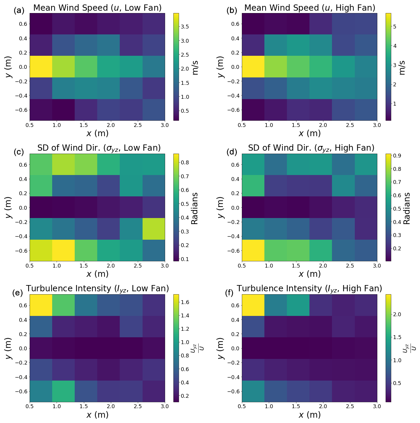
Figure C4 (a–b) Mean wind speed, (c–d) standard deviation of wind direction in the x–y plane and (e–f) turbulence intensity in the y–z plane of Experiment 2 for low-fan setting (a, c, e) and high-fan setting (b, d, f).

From these measurements, the MDB fan was able to generate a jet of pseudo-homogeneous turbulence at a range of downwind distances between 1 and 2 m. Beyond 2 m, the plume becomes unstable and can be broken easily by crosswinds, even at a high fan setting. Furthermore, the heat maps in Fig. C4 also point to the importance of measuring along the centerline (y = 0), as the effects of crosswind turbulence increase by a large amount even when only slightly off of the centerline (y > 0.3 m). Based on these results, the controlled-release experiment was conducted with the sensors at a distance of 2 m from the fan, and all of the field measurements were performed at a distance of less than 2 m.