Turbulent transport extraction in time and frequency and the estimation of eddy fluxes at high resolution

We introduce a novel framework for estimating eddy fluxes using cross-scalogram smoothing, addressing key limitations of the standard eddy-covariance method. The standard approach suffers from fixed averaging times (typically 30 min) and limited frequency resolution, which can lead to biases and an inability to capture fast dynamics. Our method, based on wavelet transforms, allows for high-resolution analysis of fluxes in both time and frequency domains. It adaptively localises turbulent scales using a metric derived from the vertical component of the Reynolds stress tensor, enabling more accurate flux estimation under varying turbulence conditions. The proposed metric is similar to the u^* and σ_w tests, but it is adapted to the time–frequency setting. By decoupling the filtering of perturbative scales from flux calculations, our approach allows for flexible averaging times. This adaptability makes it particularly suitable for studying rapid ecosystem responses to environmental changes, such as those occurring on timescales shorter than 1 h. We show application of the framework at the beech forest site Hesse (code FR-Hes) and demonstrate its relation with standard eddy-covariance calculations. The proposed method allows for varying the averaging time without impacting the filtering of the perturbative scales. It thus allows for producing estimates of CO₂, latent heat, and sensible heat fluxes with faster dynamics (e.g. with 1, 10, and 30 min averaging time). We present statistics of the 10 min averaged fluxes and show that they align well with estimates of the 30 min standard eddy-covariance method. The improved localisation of turbulent scales results in higher estimates of carbon uptake during summer (+2 ± 1 $\mathrm{\mu }\mathrm{mol}{\mathrm{m}}^{-\mathrm{2}}{\mathrm{s}}^{-\mathrm{1}}$) and a more accurate assessment of nighttime respiration compared to standard eddy-covariance estimates. The methodology is implemented in the Julia package TurbulenceFlux.jl, making it readily accessible for practical applications.

1 Introduction

The establishment of extensive networks of flux towers across the globe over the past 2 decades has proven to be a valuable asset for the scientific community and policy-makers alike. It enabled monitoring of a diverse range of ecosystems and a more detailed characterisation of their functioning (Baldocchi, 2019). This is particularly important in light of the uncertain effects of climate change on these ecosystems. In order to make the best use of the instruments and the data, standards have been established with regard to the instrumentation setup and the data processing methods. In particular, the eddy-covariance method has evolved to become a standard approach (e.g. Burba, 2022). It is now widely employed to estimate fluxes from raw measurements and is available through different software packages (Fratini and Mauder, 2014).

Standard eddy-covariance processing is constrained by its fixed averaging time, typically set to 30 or 60 min. Increasing the temporal resolution, i.e. decreasing the averaging time, is, however, not possible with the standard eddy-covariance method without impacting the filtering of the perturbative scales. Studying an alternative method that safely separates between the filtering of the perturbations (large-scale process, noise) and the flux calculation such that the averaging time may be varied may open up new research opportunities, such as studying the fast responses of plants to environmental cues (Durand et al., 2021).

The standard eddy-covariance method is based on Reynolds decomposition and the covariance operator. The Reynolds decomposition implies that signals are considered ergodic so that the rules of averaging apply (see Stull, 1988, Sect. 2.4.2). An important consequence of this is that a single parameter, the averaging time length, determines two key elements: (1) how signals are decomposed over time into mean and variable parts, where the latter should only capture local turbulent processes, and (2) the duration of the covariance operator for estimating the fluxes. However, it is clear from the experimental studies that turbulence above canopy is an intermittent process that cannot be considered ergodic (Lee et al., 2004, Chap. 8). A direct consequence is that Reynolds decomposition and the covariance operator are regarded as filtering operations. Reynolds decomposition separates signals into low- and high-frequency components, corresponding to the mean and variable parts, with the averaging time determining where this separation occurs in frequency. The ideal location is within the spectral gap between mesoscale and turbulent processes (Van der Hoven, 1957; Von Randow, 2002), such that the high-frequency component (the variable part) only captures the local turbulent transport. The covariance operator estimates a flux by correlating the variable parts over a short duration which is set to the same averaging time used during the Reynolds decomposition. Two points can be remarked. Firstly, the Reynolds decomposition does not adapt to changing conditions, i.e. a changing spectral gap, which means that the variable part of the signals may not contain at any given time the information relative to a local turbulent transport, resulting in potential biases. Secondly, the averaging time of the covariance operator is dependent on the spectral gap, yet it should only depend on the duration of the coherent structures involved in the turbulent transport. This makes it impossible to modify the operator to reach higher temporal resolutions. To overcome these limitations, an alternative decomposition that tracks the evolution of turbulence and a different estimation operator that is independent of the decomposition can be used with the goal of estimating fluxes at high temporal resolution.

The identification and extraction of localised patterns, such as microfronts, which are local and coherent structures hypothesised to contribute significantly to the flux, has been proposed to account for the intermittent nature of turbulence (Schols, 1984; Bergström and Högström, 1989). This has led to the development of numerous conditional sampling methods (e.g. Subramanian et al., 1982) for extracting patterns from turbulence time series. In that context, wavelet transforms appeared as an alternative to Reynolds decomposition and proved to be efficient in localising patterns (Mahrt and Frank, 1988; Mahrt, 1991). Collineau and Brunet (1993) first used conditional sampling with wavelet transform for studying the turbulent exchange of heat and momentum between the canopy of a pine forest and the atmosphere. The identification of structures with wavelet transforms has been exploited in many other cases: energetic eddies (Howell and Mahrt, 1994), whose approach based on energetic criteria is reminiscent of the one used by Katul and Vidakovic (1996) for the identification of detached/attached eddies (see Townsend, 1980); ${\mathrm{H}}_{\mathrm{2}}\mathrm{O}/{\mathrm{CO}}_{\mathrm{2}}$ concentrated eddies for flux partitioning (Scanlon and Albertson, 2001); upwards and downwards eddies at different heights along a shore (Attié and Durand, 2003); large-scale structures over heterogeneous terrain (Mauder et al., 2007); and short turbulent events (Schaller et al., 2017).

It has also been proposed to directly estimate fluxes from cross-scalograms, i.e. the product of the wavelet transforms of two signals, instead of focusing on particular patterns. To our knowledge, Attié and Durand (2003) and Strunin and Hiyama (2004) first exploited continuous cross-scalograms to form instantaneous fluxes in position–wavelength representation with airborne measurements, which is equivalent to a time–frequency representation for static measurements. Mauder et al. (2007) used local smoothing over cross-scalograms (see Torrence and Compo, 1998) to form averaged fluxes at different wavelengths, with their sum over wavelengths leading to flux estimates over a region. The local smoothing serves as a noise removal and estimates a local correlation (i.e. a flux) in time and frequency coordinates. This method differs from the standard eddy-covariance approach as the decomposition in different frequency bands is done separately from the actual estimation of the flux by local smoothing. It can be seen as a generalisation of the standard approach where more frequency bands are added to the Reynolds decomposition and where the covariance operator is replaced with a cross-correlation parameterised with an averaging length parameter that is independent of the decomposition. That way, the flux is estimated locally in time and frequency coordinates but without limitations in the time resolution and with sufficient frequency bands to better localise turbulent transport.

The smoothing of cross-scalograms thus seems a promising approach to overcome the limitations of the standard eddy-covariance approach. However, its use may have been hindered by the presence of various obstacles. The wide variety of available wavelet types makes selection a challenging process. The overall estimation may depend on a particular type of wavelet (Schaller et al., 2017), which raises the question of whether another family could have been more optimal. Furthermore, different types of wavelet transformations are possible, such as the orthogonal wavelet transform or the transformation of signals with redundant frames of wavelet. The decomposition should, however, conserve energy and the global flux. There is also currently no test that is adapted to time and frequency coordinates for determining that the turbulence is sufficiently developed and that the estimated flux is linked to a local turbulent transport.

In the presented work, we address the previously outlined issues. First, we establish a general framework for decomposing and estimating fluxes in time and frequency coordinates and show how the standard eddy-covariance approach or the local smoothing of cross-scalograms can be viewed as particular cases of it. We specify the conditions for ensuring that the decomposition and estimation process conserves the global flux. Next, we present a particular case of the established framework by employing a redundant frame of generalised Morse wavelets, a parameterised superfamily of wavelets that facilitates the exploration of various wavelet shapes (Lilly and Olhede, 2012). Finally, we develop a statistical test based on the Reynolds stress tensor to assess the development of turbulence in time and frequency coordinates. We present results of the proposed methodology using data acquired at the FR-Hes flux tower (Granier et al., 2008).

2 Methodology

We denote the vertical wind speed as w, the horizontal wind speeds as u and v, the temperature as θ, and a scalar of interest such as CO₂ as s. We assume that signals are observed over a period T. The Fourier transform of the signal x is denoted as $\widehat{x}$.

2.1 The standard eddy-covariance approach and its limits

We recall here the standard eddy-covariance method, before showing how it can be extended in the next section. We consider the simple case of the conservation of a passive scalar s in an incompressible flow with horizontal homogeneity, with the equation of conservation being (Sect. 3.2.6, Stull, 1988)

$$\begin{array}{}\text{(1)}& {\displaystyle \frac{\partial s}{\partial t}}+{\displaystyle \frac{\partial ws}{\partial z}}=S_{\mathrm{s}},\end{array}$$

where we neglected, for simplicity, the fluxes by diffusivity, and where S_s represents the source/sink term. The standard approach uses Reynolds decomposition to split the advective term, the second term in Eq. (1), into two terms: the eddy fluxes and fluxes due to larger-scale structures. It uses the averaging operator defined by

$$\begin{array}{}\text{(2)}& \stackrel{\mathrm{‾}}{x}\left(t\right)={\displaystyle \frac{\mathrm{1}}{T_c}}\underset{t}{\overset{t+T_c}{\int }}x\left(\mathit{\tau }\right)\mathrm{d}\mathit{\tau },\end{array}$$

where T_c is the averaging time. The observation period T composed of N averaging periods such that T = NT_c. Over a discrete time grid t = kT_c, so that $\stackrel{\mathrm{‾}}{w}$ and $\stackrel{\mathrm{‾}}{s}$ are constant over adjacent periods $[k{T}_c,(k+\mathrm{1}\left)T_c\right]$, and the averaged advective term is decomposed using the signal decomposition w = $w^{\prime }+\stackrel{\mathrm{‾}}{w}$, which results in

$$\begin{array}{}\text{(3)}& \stackrel{\mathrm{‾}}{ws}=\stackrel{\mathrm{‾}}{w^{\prime }{s}^{\prime }}+\stackrel{\mathrm{‾}}{w}\stackrel{\mathrm{‾}}{s},\end{array}$$

with the covariance operator appearing in the first term, $\stackrel{\mathrm{‾}}{w^{\prime }{s}^{\prime }}$, as

$$\begin{array}{}\text{(4)}& \stackrel{\mathrm{‾}}{w^{\prime }{s}^{\prime }}=\stackrel{\mathrm{‾}}{\left(w-\stackrel{\mathrm{‾}}{w}\right)\left(s-\stackrel{\mathrm{‾}}{s}\right)}.\end{array}$$

The averaging and decomposition of the advective term in Eq. (1) with the Reynolds decomposition at times t = kT_c results in

$$\begin{array}{}\text{(5)}& {\displaystyle \frac{\partial \stackrel{\mathrm{‾}}{s}}{\partial t}}+{\displaystyle \frac{\partial \stackrel{\mathrm{‾}}{w^{\prime }{s}^{\prime }}}{\partial z}}+{\displaystyle \frac{\partial \stackrel{\mathrm{‾}}{w}\stackrel{\mathrm{‾}}{s}}{\partial z}}=\stackrel{\mathrm{‾}}{S_{\mathrm{s}}},\end{array}$$

where $\frac{\partial \stackrel{\mathrm{‾}}{w^{\prime }{s}^{\prime }}}{\partial z}$ represents the eddy fluxes, and $\frac{\partial \stackrel{\mathrm{‾}}{w}\stackrel{\mathrm{‾}}{s}}{\partial z}$ represents the fluxes due to larger-scale structures.

To relate the eddy fluxes to the ecosystem fluxes $\stackrel{\mathrm{‾}}{S_{\mathrm{s}}}$, the storage term (first term in Eq. 5) must be taken into account along with the influence of large-scale structures. The latter can be neglected if no subsidence is assumed; i.e. $\stackrel{\mathrm{‾}}{w}$ = 0.

The Reynolds decomposition acts as a filtering operation (Kaimal et al., 1989; Lee et al., 2004, Chap. 2), where averaged quantities ($\stackrel{\mathrm{‾}}{w}$, $\stackrel{\mathrm{‾}}{s}$) results from the application of a low-pass filter and thus contains information about large-scale structures, while the variable parts, w^′, are the remaining high-frequency components of w, likely characterising small turbulent structures. This separation, i.e. the chosen averaging time T_c, should be in accordance with the spectral gap separating the turbulent scales from the larger scales. If the separation occurs outside the spectral gap, then the fluxes are biased. For example, if the averaging time T_c is such that it falls inside the band of frequencies occupied by the turbulent scales, then $\stackrel{\mathrm{‾}}{s}$ contains information about the local turbulent transport, which is lost considering only the correlation between the high-frequency components $w^{\prime }{s}^{\prime }$. The low-frequency components are influenced by external forcings which influence the position and width of the spectral gap throughout the day (Von Randow, 2002; Lee et al., 2004). Thus, at any given time, it is unlikely that the high-frequency part contains all of or only the information relative to turbulent transport. The averaging time used for the Reynolds decomposition should, hence, adapt dynamically to measurement conditions.

The averaging time of the standard eddy-covariance approach places constraints on both the manner in which signals are decomposed and the estimation period used to calculate eddy fluxes via the covariance operator. Alternatively, the decomposition and estimation processes could be parameterised independently. The former would be influenced by the location of the spectral gap, while the latter would depend on the time support (physical size) of the coherent structures.

2.2 An extension of the standard approach with a higher resolution in time and frequency

To overcome the aforementioned problems of the standard eddy-covariance approach, the frequency band occupied by the turbulent scales needs to be estimated at any given time.

The proposed approach is to decompose the data into several frequency bands and decide at any given time which portion of these frequency bands will be used to estimate the eddy fluxes.

Here, we split the advective term into more frequency bands instead of the two frequency bands originally present in the Reynolds decomposition. With L being such frequency bands spanning all frequencies, we denote as w_l and s_l the filtered versions of w and s, where w_l corresponds to the analysis in the lth frequency band. An averaging operator [⋅]_ϕ is introduced, where [x]_ϕ = x×ϕ is the convolution between the signal x and the averaging function ϕ. Similarly to Eq. (3), the advective term averaged here with ϕ is expanded using

$$\begin{array}{}\text{(6)}& {\left[ws\right]}_{\mathit{\varphi }}\simeq \sum _{l=\mathrm{1}}^L{\left[w_l{s}_l\right]}_{\mathit{\varphi }}.\end{array}$$

We present in Appendix A5 an analysis of the viability of this approximation as a function of some parameters of the decomposition that will be detailed in Sect. 2.4. Then the eddy fluxes are localised through time and frequency using this decomposition. A “turbulence” mask is introduced: 𝒳(t,l), $t\in [\mathrm{0},T]$, $l\in \mathit{\{}\mathrm{0},\mathrm{\dots },L-\mathrm{1}\mathit{\}}$, where 𝒳(t,l) = 1 indicates that the frequency band l contains turbulent eddies at time t, and it is 0 otherwise. The advective term is decomposed into turbulent eddy fluxes and other fluxes, encompassing those generated by large-scale processes and noise:

$$\begin{array}{}\text{(7)}& \begin{array}{rl}{\left[ws\right]}_{\mathit{\varphi }}\left(t\right)& \simeq \sum _{l=\mathrm{1}}^L{\left[w_l{s}_l\right]}_{\mathit{\varphi }}=\underset{\text{Eddy fluxes}}{\underbrace{\sum _{l=\mathrm{1}}^L\mathcal{X}(t,l){\left[w_l{s}_l\right]}_{\mathit{\varphi }}\left(t\right)}}\\ & +\underset{\text{Large-scale fluxes}+\text{noise}}{\underbrace{\sum _{l=\mathrm{1}}^L\left(\mathrm{1}-\mathcal{X}(t,l)\right){\left[w_l{s}_l\right]}_{\mathit{\varphi }}\left(t\right)}}.\end{array}\end{array}$$

The conservation of mass equation then writes as

$$\begin{array}{}\text{(8)}& \begin{array}{rl}{\displaystyle \frac{\partial {\left[s\right]}_{\mathit{\varphi }}}{\partial t}}& +\sum _{l=\mathrm{1}}^L\mathcal{X}(t,l){\displaystyle \frac{\partial {\left[w_l{s}_l\right]}_{\mathit{\varphi }}}{\partial z}}\\ & +\sum _{l=\mathrm{1}}^L(\mathrm{1}-\mathcal{X}(t,l\left)\right){\displaystyle \frac{\partial {\left[w_l{s}_l\right]}_{\mathit{\varphi }}}{\partial z}}={\left[S_{\mathrm{s}}\right]}_{\mathit{\varphi }}.\end{array}\end{array}$$

To relate the eddy fluxes to the ecosystem fluxes, the storage term (first term) and the influence of large-scale fluxes (third term) need to be taken into account.

The proposed decomposition of the advective term (Eq. 6) is similar to the decomposition made in Reynolds decomposition (Eq. 3), where the filters are the averaging operator of Eq. (2) and its high-pass filter counterpart.

The local smoothing of cross-scalograms (Mauder et al., 2007) is also a particular decomposition of the advective term. The filtered versions w_l and s_l are the wavelet decompositions of signals at particular scales l (see Torrence and Compo, 1998). It leads to the formation of cross-scalograms with the product w_ls_l and to local estimation of the flux in time and frequency coordinates through averaging with ${\left[w_l{s}_l\right]}_{\mathit{\varphi }}$.

In the next section (Sect. 2.3), we elaborate on a general framework that presents sufficient conditions for the filters and the averaging operator so that the decomposition into different frequency bands conserves the global flux, i.e. to verify that

$$\begin{array}{}\text{(9)}& \underset{\mathrm{0}}{\overset{T}{\int }}\sum _{l=\mathrm{0}}^L{\left[w_l{s}_l\right]}_{\mathit{\varphi }}\left(\mathit{\tau }\right)\mathrm{d}\mathit{\tau }=\underset{\mathrm{0}}{\overset{T}{\int }}w\left(\mathit{\tau }\right)s\left(\mathit{\tau }\right)d\mathit{\tau }.\end{array}$$

Later, in Sect. 2.4, we show how to implement that framework by relying on generalised Morse wavelets. Finally, we introduce in Sect. 2.5 a metric based on the vertical amplitude of the Reynolds stress tensor for identifying the vertical turbulent transport and estimating the turbulence mask 𝒳.

2.3 A general framework for decomposing fluxes in time–frequency space

The proposed framework chooses a set of filters {ψ_l}_l indexed with $l\in \mathit{\{}\mathrm{0},\mathrm{\dots },L-\mathrm{1}\mathit{\}}$ as well as an averaging function ϕ. These filters could be, but are not limited to, the well-known wavelets (Mallat, 2009). We start by filtering the signals with the set of filters {ψ_l}_l, leading to a decomposition in frequency bands. Each filter ψ_l occupies a particular frequency band indexed with parameter l. The filtered versions of w and s are computed using

$$\begin{array}{}\text{(10)}& w_l\left(t\right)=\underset{\mathrm{0}}{\overset{T}{\int }}w\left(\mathit{\tau }\right){\mathit{\psi }}_l(t-\mathit{\tau })\mathrm{d}\mathit{\tau }=\left(w\times {\mathit{\psi }}_l\right)\left(t\right),\end{array}$$

with x×y denoting a convolution between the two signals x and y.

For each frequency band l and at each time t, a local flux in time and frequency F_s(t,l) is estimated using the averaging function ϕ:

$$\begin{array}{}\text{(11)}& \begin{array}{rl}& {\mathrm{F}}_{\mathrm{s}}(t,l)=\underset{\mathrm{0}}{\overset{T}{\int }}{w}_l\left(\mathit{\tau }\right)s_l\left(\mathit{\tau }\right)\mathit{\varphi }(t-\mathit{\tau })\mathrm{d}\mathit{\tau }=\left(w_l{s}_l\times \mathit{\varphi }\right)\left(t\right)\\ & ={\left[w_l{s}_l\right]}_{\mathit{\varphi }}\left(t\right),\end{array}\end{array}$$

which is the convolution of the product w_ls_l with the averaging function ϕ at time t.

We impose the following conditions on the filters and the averaging function:

Condition 2.1. The decomposition with filters {ψ_l} is “self-dual” (see Mallat, 2009, Sect. 5.1.5); i.e. the energy spectral density of all filters sums to one:

$$\begin{array}{}\text{(12)}& \sum _{l=\mathrm{1}}^L{\left|\widehat{{\mathit{\psi }}_l}\left(\mathit{\nu }\right)\right|}^{\mathrm{2}}=\mathrm{1}\forall \mathit{\nu },\end{array}$$

with $\widehat{{\mathit{\psi }}_l}\left(\mathit{\nu }\right)$ being the Fourier transform of ψ_l at frequency ν.

Condition 2.2. The averaging function ϕ is positive and integrates to a constant unit signal over the observation period T:

$$\begin{array}{}\text{(13)}& \underset{\mathrm{0}}{\overset{T}{\int }}\mathit{\varphi }(\mathit{\tau }-t)\mathrm{d}\mathit{\tau }=\mathrm{1}\forall t\in [\mathrm{0},T].\end{array}$$

A Gaussian window can, for example, be chosen as the averaging function where the variance controls the level of smoothing of the estimated fluxes.

Conditions 2.1 and 2.2 are sufficient conditions (see Appendix A1) so that the global flux,

$$\begin{array}{}\text{(14)}& F_{\mathrm{s}}^T={\displaystyle \frac{\mathrm{1}}{T}}\underset{\mathrm{0}}{\overset{T}{\int }}w\left(\mathit{\tau }\right)s\left(\mathit{\tau }\right)\mathrm{d}\mathit{\tau },\end{array}$$

can be recovered by summing over all filters and integrating through time F_s(t,l):

$$\begin{array}{}\text{(15)}& {\displaystyle \frac{\mathrm{1}}{T}}\underset{\mathrm{0}}{\overset{T}{\int }}\sum _{l=\mathrm{1}}^L{F}_{\mathrm{s}}(\mathit{\tau },l)\mathrm{d}\mathit{\tau }=F_{\mathrm{s}}^T.\end{array}$$

2.4 Time and frequency decomposition of fluxes with generalised Morse wavelets

Choosing a particular set of filters depends on the application and generally requires precise insights on the property of the signals under study. The turbulent process is scale invariant, and with Taylor's hypothesis of frozen turbulence it follows that fast-varying oscillations are associated with eddies of small size and inversely that a slow-varying signal is related to eddies of larger size (Stull, 1988; Powell and Elderkin, 1974). Wavelets share the same property, i.e. if ψ(t) is a wavelet and ψ_a(t) = $\mathit{\psi }(t/a)/\sqrt{a}$ is a scaled version, then the frequency peak of ψ(t) is scaled by a factor a. In other words, a wavelet at small scale captures fast-varying oscillations over short periods of time, and a wavelet at large scale captures fast variations. Thus, the scale of a wavelet, which is proportional to the length of its time support, can be related to the physical size of eddies.

Instead of making an arbitrary choice of a particular family of wavelets such as Mexican hat or Morlet wavelets, we base our approach on generalised Morse wavelets (Lilly and Olhede, 2009, 2012), which is a parameterised superfamily that encompasses a wide variety of wavelets. It is a two-parameter family of analytic wavelets defined in frequency by

$$\begin{array}{}\text{(16)}& {\widehat{\mathit{\psi }}}_{\mathit{\beta },\mathit{\gamma }}\left(\mathit{\nu }\right)=C{\mathit{\nu }}^{\mathit{\beta }}{e}^{-{\mathit{\nu }}^{\mathit{\gamma }}},\mathit{\nu },\mathit{\beta },\mathit{\gamma }>\mathrm{0},\end{array}$$

with C being a normalisation constant. β and γ are two shape parameters that control notably the frequency peak, the kurtosis, and skewness of the wavelet spectrum (for more details see Lilly and Olhede, 2009).

The practical advantage of using generalised Morse wavelets is that it avoids having to choose between many different wavelet families, each with its own implementation details. Here, the shape parameters β and γ can be changed to adapt the decomposition. Perrier et al. (1995) showed that β should not be smaller than $(\mathit{\alpha }-\mathrm{1})/\mathrm{2}$, where α is the exponent of the energy spectral density of the analysed signal. This gives the lower limit of $\mathrm{1}/\mathrm{3}$ for β if we assume the Kolmogorov–Obukhov spectrum where α = $\mathrm{5}/\mathrm{3}$. We chose the parameters β = 2 and γ = 3 as they produce wavelets with a good energy concentration in time and frequency space (Lilly and Olhede, 2012) and consequently localises different turbulent events well.

Equation (16) is used to define a mother wavelet, using the chosen shape parameters, which is upscaled iteratively to form a set of filters. Starting at the lowest scale a₀ of the mother wavelet, J⋅Q upscaled versions with scales a_i = $a_{\mathrm{0}}{\mathrm{2}}^{i/Q}$ and $\mathrm{0}\le i\le JQ-\mathrm{1}$ are iteratively constructed with J being the number of octaves and with Q being the number of inter-octaves. This leads to a set of filters whose frequency peaks are logarithmically spaced by a factor ${\mathrm{2}}^{-i/Q}$ from the highest to the lowest frequency. Q controls how resolved the analysis between two octaves is, while J controls how far the analysis goes towards the lowest frequency (which is ultimately limited by the length of the observation period). The wavelet frequency peaks are at ν_i = $\frac{\mathrm{1}}{a_i}{\left(\mathit{\beta }/\mathit{\gamma }\right)}^{\mathrm{1}/\mathit{\gamma }}$. Each wavelet is normalised in frequency by the value at its frequency peak. In practice, wavelets at the highest scales may be discarded if their frequency spectrum is not sampled well enough, leading to a lower number, K < JQ, of wavelet filters. Since generalised Morse wavelets are first instantiated in the frequency domain, poorly sampled wavelets appear at the lower end of the spectrum; thus, a limiting frequency can be chosen, e.g. ν_min = $\mathrm{2}{F}_{\mathrm{s}}/N$, where F_s is the sampling frequency and where N is the sample size so that wavelets with frequency peaks below that limiting frequency are discarded. Finally, a low-pass filter, noted h in the following, is added to our current set of wavelet filters so that the lowest frequency region not yet spanned by the wavelets is captured. We use a simple Gaussian filter for the low-pass filter with a −3 dB cutoff frequency set at the lowest frequency peak of the set of wavelet filters. This leads to a set of L = K + 1 filters composed of K wavelets $\mathit{\left\{}{\mathit{\psi }}_{a_i}\right|a_i=a_{\mathrm{0}}{\mathrm{2}}^{i/Q},\mathrm{0}\le i\le K-\mathrm{1}\mathit{\}}$ and a low-pass filter that we note as h. To satisfy condition 2.1, each wavelet and the low-pass filter has its frequency spectrum divided by

$$\begin{array}{}\text{(17)}& G\left(\mathit{\nu }\right)=\sqrt{{\left|\widehat{h}\left(\mathit{\nu }\right)\right|}^{\mathrm{2}}+\sum _{\mathrm{0}\le i\le K-\mathrm{1}}{\left|{\widehat{\mathit{\psi }}}_{a_i}\left(\mathit{\nu }\right)\right|}^{\mathrm{2}}}.\end{array}$$

After normalisation, we obtain a set of filters that respects condition 2.1 and has the same characteristics as wavelets. The procedure keeps an important property for the analysis of turbulence: the effective scale of the filters (time support length) still varies in inverse proportion to their frequency peaks. Thus, the theoretical frequency peaks of the initial set of wavelets can still be used as proxies for the scales of the filters. We give in Appendix A2 more details on the impact of this normalisation step.

Note that the normalisation of Eq. (17), which ensures global flux conservation, is motivated by the wavelet frame theory (see Mallat, 2009, Sect. 5.1.5) that can generally be applied to any set of filters. It is different from the C_ψ reconstruction constant found in Torrence and Compo (1998). The latter comes from the discretisation of the admissibility condition for continuous wavelet transforms. However, for practical applications where signals are always decomposed on a discrete set of scales, wavelet frame theory applies rather than the theory of continuous wavelet transforms.

With Taylor's frozen turbulence assumption and the property that the frequency peaks of wavelets are linked to their scale, the filtering of any signal with a wavelet ψ with frequency peak ν is equivalent to an analysis at a hypothetical eddy scale $\mathit{\lambda }\propto \left|u\right|/\mathit{\nu }$ with |u| being the mean amplitude of the wind. Using in our case the aerodynamic height z−d, where z is the measurement height and where d is the displacement height, the normalised frequency is given by

$$\begin{array}{}\text{(18)}& \mathit{\eta }={\displaystyle \frac{(z-d)}{\left|u\right|/\mathit{\nu }}}={\displaystyle \frac{(z-d)\mathit{\nu }}{\left|u\right|}}.\end{array}$$

This normalised frequency can be interpreted as the ratio between a height above “ground” of the observations and the size of a hypothetical eddy at time t and oscillating frequency ν. High normalised frequencies indicate eddies of small sizes with fast oscillations, and inversely low normalised frequencies indicate large eddies with slow oscillations.

For the rest of the paper, we will drop time vs. frequency band index coordinates such as in Eq. (11), and we use time vs. normalised frequency coordinates where η will be the frequency peak of the wavelet covering the lth frequency band. For visualisations in Sect. 3, we allowed the normalised frequency η to be time dependent as the mean amplitude of the wind |u| varies through time; thus, time and frequency decompositions will be presented in Lagrangian coordinates (t,η(t)).

2.5 Identification of vertical turbulent transport in time and frequency

With the standard eddy-covariance method, different statistics has been proposed to assess the quality of the estimated flux (see Foken, 2017, Sect. 4.3.2). Flux variance similarity (or integral turbulence characteristics), friction velocity u^*, and wind speed variance σ_w have been proposed to test turbulence development (see Foken and Wichura, 1996).

Here, an alternative approach adapted to time and frequency coordinates is proposed. The vertical amplitude of the Reynolds stress tensor is used to identify in time and frequency coordinates the vertical turbulent processes. It assesses across time and frequency the contributions by eddies in the vertical deformations and vertical momentum of an elementary volume under observation. To do so, we propose the following metric:

$$\begin{array}{}\text{(19)}& {\mathit{\tau }}_{\mathrm{w}}(t,\mathit{\eta })=\sqrt{F_u(t,\mathit{\eta }{)}^{\mathrm{2}}+F_v(t,\mathit{\eta }{)}^{\mathrm{2}}+F_{\mathrm{w}}(t,\mathit{\eta }{)}^{\mathrm{2}}}.\end{array}$$

where F_u, F_v, and F_w are the vertical kinematic fluxes computed using Eq. (11) at time t and normalised frequency η.

This quantity is related to friction velocity u^* and the variance of vertical wind speed σ_w. With Reynolds decomposition, it could be written as $\sqrt{{\stackrel{\mathrm{‾}}{u^{\prime }{w}^{\prime }}}^{\mathrm{2}}+{\stackrel{\mathrm{‾}}{u^{\prime }{v}^{\prime }}}^{\mathrm{2}}+{\stackrel{\mathrm{‾}}{w^{\prime }{w}^{\prime }}}^{\mathrm{2}}}=\sqrt{{u^{*}}^{\mathrm{4}}+{{\mathit{\sigma }}_{\mathrm{w}}}^{\mathrm{4}}}$, and Eq. (19) is an extension to a time and frequency representation with higher resolution.

Our methodology to identify time and frequency regions is based on the analysis of τ_w. τ_w is large in time and in frequency regions with vertical turbulent structures due to buoyancy or mechanical shear. In order to identify such regions, a threshold δ_τ is set to find all points $(t^{*},{\mathit{\eta }}^{*})$ such that ${\mathit{\tau }}_{\mathrm{w}}(t^{*},{\mathit{\eta }}^{*})>{\mathit{\delta }}_{\mathit{\tau }}$. In the presented results (see Sect. 3.2), the threshold δ_τ was set manually by examining how the distribution of sensible heat deviates as the amplitude of τ_w increases. Above this threshold, the probability of heat exchange occurring (either positive or negative, depending on the stratification) should stay high. We found its value to be approximately 10⁻³ m² s⁻². This first step identifies all time and frequency coordinates where vertical processes affect the measured volume of air, thereby removing noise. However, slow-varying trends may still be present, potentially originating from inhomogeneities in the advected scalar field or from subsidence. An additional step is necessary to remove these unwanted regions in time–frequency space. In the spectral analysis of turbulence, this step is equivalent to finding a spectral gap between the turbulent scales and the contributions of larger scales (Powell and Elderkin, 1974). The main difference here is that we estimate a time-dependent spectral gap that is adapted to non-stationary settings.

We analyse the Laplacian (second derivatives) of log τ_w to find the separating spectral gap. High values of the Laplacian suggest the presence of minima in regions that are primarily affected by noise and spurious correlations. We expect that such regions exist in-between the turbulent scales and the larger scales. We identify all time and frequency points 𝒰 = $\left\{(t,\mathit{\eta })\left|\mathrm{\Delta }\log {\mathit{\tau }}_{\mathrm{w}}\right(t,\mathit{\eta })>{\mathit{\delta }}_{\mathrm{\Delta }{\mathit{\tau }}_{\mathrm{w}}}\right\}$ with a Laplacian larger than a given threshold ${\mathit{\delta }}_{\mathrm{\Delta }{\mathit{\tau }}_{\mathrm{w}}}$. We fit a curve to the selected points 𝒰 with a locally weighted regression method (Cleveland and Devlin, 1988), which is the time-varying spectral gap η_*(t) separating the time and frequency regions with local turbulent transport from the influence of larger-scale structures. We found that the method is not very sensitive to the value of the threshold ${\mathit{\delta }}_{\mathrm{\Delta }{\mathit{\tau }}_{\mathrm{w}}}$, and we set it to 1 here. It has to be sufficiently small to select a sufficient number of points such that the locally weighted regression method passes preferably in regions with a high number of detected minima.

The above steps lead to the creation of the turbulence mask introduced in Eq. (8), identifying time–frequency regions with sufficiently developed turbulence:

$$\begin{array}{}\text{(20)}& \mathcal{X}(t,\mathit{\eta })=\left\{\begin{array}{ll}\mathrm{1}& \text{if}\mathit{\eta }>{\mathit{\eta }}_{*}\left(t\right)\text{and}{\mathit{\tau }}_{\mathrm{w}}(t,\mathit{\eta })>{\mathit{\delta }}_{\mathit{\tau }},\\ \mathrm{0}& \text{otherwise}.\end{array}\right.\end{array}$$

This turbulence mask covers the time and frequency regions with normalised frequencies above the estimated time-dependent spectral gap η_* and with sufficiently strong vertical kinematic fluxes. Note that the turbulence mask is indexed with time and normalised frequency (t,η) here, while it is indexed with time and the index of the band of frequency (t,l) in Eq. (8). We relate η to the frequency peak of the wavelet covering the lth frequency band.

2.6 Summary of proposed methodology

We depict in Fig. 1 a summary of the proposed methodology. First, a frame of wavelets with conservative property is used to decompose wind speeds and other scalars in time and frequency. Cross-scalograms are formed as the product of the signal decompositions and time averaged to form fluxes resolved in time and frequency. Vertical kinematic fluxes in time and frequency coordinates are used to localise the time–frequency regions with local turbulent transport. This leads to the creation of a turbulence mask that is applied over time- and frequency-decomposed scalar fluxes to integrate time-resolved scalar fluxes.

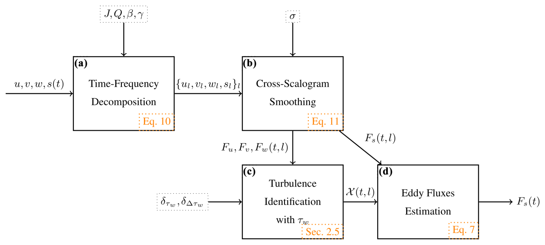
Figure 1 Summary diagram of the proposed methodology for estimating fluxes from turbulent transport. (a) Signals are decomposed in time–frequency space using a set of filters composed of wavelets and a low-pass filter. They are initialised and normalised according to Eq. (17) to have a conservative property. (b) Cross-scalograms are formed and averaged through time using an averaging function of size σ respecting condition 2.2. (c) Given vertical kinematic fluxes the metric τ_w of Eq. (19) is computed and a turbulence mask 𝒳 identifying the vertical turbulent transport is inferred. (d) The flux of scalar s is estimated by integrating through frequencies the vertical flux F_s(t,l) in time and frequency coordinates according to the turbulence mask 𝒳.

The eddy flux F_s in Eq. (7) is calculated by combining Eqs. (11) and (20) as follows:

$$F_{\mathrm{s}}\left(t\right)=\sum _{\mathit{\eta }}\mathcal{X}(t,\mathit{\eta })F_{\mathrm{s}}(t,\mathit{\eta }),$$

where F_s(t,η) is the time- and frequency-decomposed flux, and 𝒳(t,η) is the turbulent mask at time t and normalised frequency η. Each scale of the decomposed flux in Eq. (11) is obtained by filtering the signals using Eq. (10). Their products are then smoothed with a Gaussian window parameterised by an averaging length σ. Wavelets are generated via Eq. (16), with their Fourier transform normalised according to Eq. (17).

The approach requires several parameters. (1) β and γ determine the shape of the generalised Morse wavelet. (2) J and Q control the overall resolution in frequency of the decomposition. (3) σ is the width of the averaging function. (4) The two thresholds ${\mathit{\delta }}_{{\mathit{\tau }}_{\mathrm{w}}}$ and ${\mathit{\delta }}_{\mathrm{\Delta }{\mathit{\tau }}_{\mathrm{w}}}$ condition the identification of the local turbulent process in time–frequency coordinates.

The wavelet parameters need to be shared across all time and frequency decompositions to keep the same coordinate system. In practice, 20 Hz signals are used to form the cross-scalograms with consistent resolution over time and a frequency resolution defined by the parameters J and Q. After smoothing the cross-scalograms, they may be sub-sampled at a resolution of, for example, 1 min. To reconstruct the original 20 Hz versions of the cross-scalograms, the averaging time should be at least twice the sampling step.

The averaging parameter σ may differ when computing τ_w for identifying the turbulence mask and when computing the smoothed cross-scalograms of scalar fluxes. With the current method for establishing the turbulence mask, it is preferable to use a higher or equal averaging time for the turbulence mask compared to that used for resolving the scalar fluxes. This approach slightly overestimates the size of the turbulent time–frequency regions, ensuring that all eddy fluxes are contained within it. For example, the turbulence mask may be inferred from slowly varying vertical kinematic fluxes, using σ = 30 min, while the fluxes themselves can be calculated using a shorter averaging time, such as, for example, using σ = 10 min.

3 Results

The methodology is applied on data acquired at the FR-Hes flux tower (Granier et al., 2008), a class 1 ecosystem station of the Integrated Carbon Observation System (ICOS). The analysis was performed over the whole year 2022. Here, we present selected days and statistics over 8 h periods for day and night during summer (10–19 June 2022) and winter (3–11 March 2022). The tower is situated in a beech forest with a roughly flat terrain (< 3 % slope). The ICOS standard instrumentation (see Rebmann et al., 2018) is installed at FR-Hes with a LI-7200rs gas analyser (LI-COR Biosciences, Lincoln, USA) and an HS-50 anemometer (Gill Instruments Ltd, Lymington, UK). All signals are acquired at 20 Hz at a height of 30.8 m above ground with a canopy height of about 21.5 m in 2022. The displacement height was estimated to be 14.7 m using $\mathrm{2}/\mathrm{3}$ of canopy height (Raupach, 1994). These heights are used to compute normalised frequencies (Eq. 18). All fluxes were calculated in batches of 24 h raw data, either centred around noon or around midnight. The filtering with wavelets and averaging creates errors at the borders of the observation period (see Torrence and Compo, 1998). The standard deviations in time of the wavelets and the averaging filter are summed for each frequency band to estimate the erroneous time frame at the edges of the 20 h periods. We take the maximum across frequency bands of the standard deviations to get the size of the time window to remove from the results. The time period is estimated to be 2 h on each side, which results in flux estimates of 20 h for each 24 h observational period.

All time and frequency decompositions are computed using the wavelets of Sect. 2.4. The shape parameters for the generalised Morse wavelets are taken as β = 2 and γ = 3, as explained before. The wavelets are positioned according to their frequency peaks. Since data are acquired at 20 Hz, the frequency peak of the first wavelet is initiated at 10 Hz, and subsequent wavelets are scaled up by a factor of ${\mathrm{2}}^{\mathrm{1}/Q}$ with Q = 4 until the minimum frequency peak of $F_{\mathrm{s}}\mathrm{2}/N$ is reached, where N is the number of samples and where F_s is the sampling frequency of 20 Hz. With 24 h long observation periods and a sampling frequency of 20 Hz, the limiting frequency corresponds to a time period of 12 h. The low-pass filter then spans the remaining frequency band below that limiting frequency, thus capturing processes with oscillation periods larger than 12 h. Since we are mostly interested in the study of eddy fluxes here, this frequency band is always discarded. Different sizes of the averaging function are used to compute the metric τ_w and to estimate the fluxes in time (see Eq. 11 and Sect. 2.5). We choose a Gaussian window with deviation σ = 30 min for τ_w and σ = 10 min for the estimation of the scalar fluxes. After averaging, i.e. after step (c) in Fig. 1, fluxes in time and frequency coordinates have a temporal resolution of 20 Hz and around 70 frequency bands (depending on the original size of the signals). The decompositions are sub-sampled at a 1 min time interval to save memory. In the following, the fluxes will be presented in time versus normalised frequency coordinates (t,η), instead of time versus the index of a frequency band (t,l) as in Eq. (8), where the normalised frequency is the frequency peak of the wavelet covering the lth frequency band.

We compare results obtained using our method (high-resolution turbulence mask, HRTM) to the estimations without turbulence mask (HR), corresponding to a wavelet-based estimated flux that integrates over all scales, as well as to the estimations with the standard eddy-covariance approach with 30 min time averaging (EC30). For information and to better understand the presented results, the flux estimation with the 30 min standard eddy covariance is roughly equivalent to integrating all the flux from the normalised frequency η = $\mathrm{5}\times {\mathrm{10}}^{-\mathrm{3}}$ if a time length of order $(z-d)/\left|u\right|\simeq$ 10 s (see Eq. 18) is assumed.

All fluxes are presented without frequency corrections in amplitude (see Burba, 2022), with H₂O and CO₂ concentration signals being corrected for time lags with wind anemometer data. H₂O and CO₂ concentration signals were shifted to maximise total correlation with vertical wind velocity for each 24 h period by using only data in the 0.1 to 1 Hz frequency band. This range was chosen to reduce the potential influence of low-frequency trends in the estimation of the time lag transporting at the same time sufficient information about the turbulent transport. It corresponds roughly to the normalised frequency range η = 1 to η = 10. The estimated time lags were 260 ± 125 ms for CO₂ and 400 ± 130 ms for H₂O on average. Sensible heat fluxes use the so-called sonic temperature from the anemometer. It is thus not corrected for humidity (see p. 42 in Dijk et al., 2004). Frequency correction and humidity correction are foreseen to be included in the method in the near future. Finally, the WPL (Webb, Pearman, and Leuning) correction (Webb et al., 1980) is not required in our case as the LI-7200rs gas analyser outputs dry mole fractions (see Burba, 2022, Sect. 4.7).

The methodology has been implemented in the Julia package TurbulenceFlux.jl.

3.1 Detailed example of the estimation of CO₂ flux

We present in Fig. 2 a detailed example of the estimation of CO₂ flux on 15 June 2022, a day characterised by sunny conditions with no precipitation. All time–frequency decompositions and the estimated fluxes are presented with a time step of 1 min. Panel (a) displays the τ_w metric, calculated using an averaging time of σ = 30 min, while panel (b) shows its Laplacian. Panel (c) presents the cross-scalogram of the CO₂ flux, calculated with an averaging time of σ = 10 min. Finally, panel (d) shows the estimated CO₂ flux (solid line) after applying the turbulent mask, along with fluxes calculated using other averaging times (σ = 1 min and σ = 30 min, represented by dashed and dotted lines, respectively).

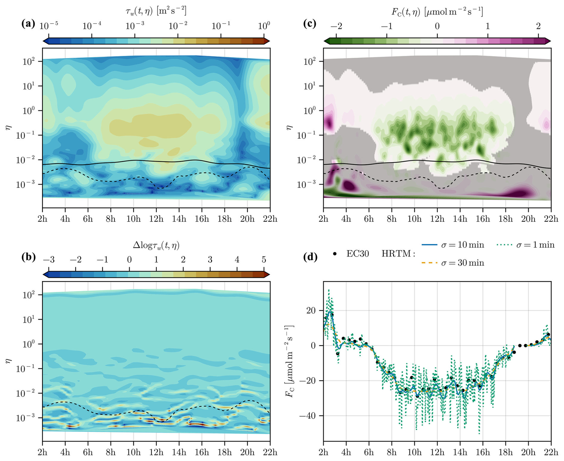
Figure 2 Turbulent transport identification and estimation of CO₂ flux on 15 June 2022. All time and frequency analyses are visualised in normalised frequencies η vs. time over 24 h. (a) Time and frequency decomposition of the amplitude of the vertical component of the Reynolds stress tensor τ_w. (b) Laplacian of log τ_w in time and frequency space with an estimated time-varying spectral gap (dashed line) separating the turbulent transport at small scales from structures at larger scales. (c) CO₂ flux in time and frequency space with a turbulence mask derived from analyses of panels (a) and (b). A time varying 30 min spectral gap associated with the frequency separation of the standard eddy-covariance method (EC30) is also shown (solid line). (d) HRTM CO₂ estimations with different averaging times against the standard 30 min eddy-covariance method (EC30).

The τ_w metric (Sect. 2.5) in Fig. 2a identifies the vertical turbulent structures in time and frequency here obtained with an averaging length of 30 min. Time and frequency regions of high intensity (> 10⁻² m² s⁻²) are approximately located from η = 10⁻² to η = 10, with a noticeable difference between day and night as well as the times of sunrise and sunset. This difference can be explained by the type of turbulence at play: from 6 to 18 h the turbulence is mostly created by buoyancy within the range η = 10⁻² to η = 1, while from 20 to 4 h the turbulence originates from mechanical shear and is located in the range η = 10⁻¹ to η = 10. Large regions of high intensity from η = 10⁻² to η = 10 indicate some stability in the physical process at play. Below η = 10⁻¹ at night and η = 10⁻² during the day, τ_w has generally low amplitude (10⁻⁴ m² s⁻²) with isolated and small time–frequency regions of medium intensity (10⁻³ m² s⁻²). Below these ranges in η, large-scale structures (η ≃ 10⁻³) intermittently apply vertical stress over short periods of time (< 2 h).

Similar patterns were observed on different days throughout the year at FR-Hes, which motivated the following assumptions: (1) vertical turbulent transport shows large and coherent regions of high intensity in the metric τ_w at frequencies corresponding to eddies with sizes around the distance of the sensor to the roughness elements, i.e. from the measurement height to the displacement height and hence around normalised frequencies of η = 1; (2) a region of low amplitude exists in τ_w at small normalised frequencies and hence large eddies, i.e. a spectral gap between the turbulent region of (1) and a region influenced by large-scale processes; and (3) small and isolated time–frequency regions of medium intensity at large scales (η < 10⁻²) are considered too unstable, and the scale is too large such that they could be part of local vertical turbulent transport.

Hence, the high-intensity regions of (1) are identified using a threshold τ_w > 10⁻³ m² s⁻², as shown by the dashed line in Fig. 2b. The spectral gap in time–frequency space is identified by the maxima of the Laplacian of log τ_w (see Sect. 2.5), as can be seen by the dashed line in Fig. 2b. It rejects most of the small size and medium-intensity regions situated below the spectral gap in τ_w (Fig. 2a). Together, they define the mask identifying local turbulent transport relevant for estimation of ecosystem fluxes, which is the bright region in Fig. 2c. The mask is shown on top of the CO₂ flux decomposed in time and frequency space, highlighting the time and frequency regions with sufficiently developed local turbulence. Note that the smoothed CO₂ flux cross-scalogram used an averaging kernel of 10 min compared to 30 min for the determination of the turbulence mask. One can see that the mask covers time–frequency regions of high amplitude of positive and negative CO₂ fluxes. The turbulence mask highlights the CO₂ respiration process at night and CO₂ assimilation during daytime. It rejects regions of large CO₂ fluxes at low frequencies around η = 10⁻³ mostly from dusk into the night. The CO₂ flux in time and frequency coordinates is integrated along the frequency scale, leading to high-resolution CO₂ fluxes shown in Fig. 2d. We obtain a high-resolution estimation (HRTM) that follows well the standard eddy-covariance estimation (EC30). In practice, the standard eddy covariance with 30 min resolution (EC30) is approximately equivalent to integrating all the CO₂ fluxes from η = 10⁻² to η = 10². This is why in this particular case one does not see the influence of the CO₂ fluxes at larger scales (η = 10⁻³) at night in the EC30 estimates. It also looks like EC30 misses some carbon uptake in the middle of the day due to the fixed integration time of 30 min. Both methods estimate a negative CO₂ flux at 3 h at night. This comes from the small time and frequency region of negative CO₂ flux at η = 10⁻² to η = 10⁻¹. The effect is more pronounced in EC30, but also our method is not inert against this intermittency. If the turbulence mask does not cover any frequency bands at a given time, meaning no turbulence is detected, we consider the calculated flux to be undefined, as integration occurs over an empty frequency domain. This can be seen around 19 h in Fig. 2d, where HRTM is undefined due to the lack of frequency bands covered by the turbulence mask in Fig. 2c. In the context of eddy-flux estimation, the flux could be treated as zero, since no turbulent coherent structures are identified to mix the air layers. When estimating ecosystem fluxes, this is a typical scenario where it is important to account for the storage term.

3.2 Statistics of τ_w and time- and frequency-decomposed sensible heat flux

We show in Fig. 3 the probability densities of τ_w against η (top row) and against the sensible heat flux F_H (bottom row) during day and night periods in summer (left and right columns, respectively). The probability densities are estimated with a kernel density estimation method. The evolution of τ_w against η presents a shortening of the frequency bandwidth occupied by the turbulent scales as it transitions from an unstable stratification to a stable stratification. The spectrum of the vertical velocity and the co-spectrum of u⋅w also share that characteristic (Kaimal and Finnigan, 1994, Sect. 2.5 and 2.9). During daytime and unstable stratification (Fig. 3a), τ_w has a concave shape from η = 10⁻³ to η = 10² with a maximum around η = 10⁻¹. During nighttime and stable stratification (Fig. 3c), the distribution of τ_w against η has its concave shape moved to higher frequencies with a maximum around η = 1 and located from η = 10⁻¹ to η = 10². In comparison with daytime conditions, the nighttime density of τ_w against η presents a greater variability: it has a stronger spread along τ_w and a less clearly defined shape. In particular, the range η = 10⁻⁴ to η = 10⁻¹ is suspected to be influenced by large-scale structures with a random behaviour. Note that our visualisations of τ_w against η are not normalised against a quantity such as the friction velocity, nor is it weighted by the frequency as is usually done in studies of spectra and co-spectra of turbulence.

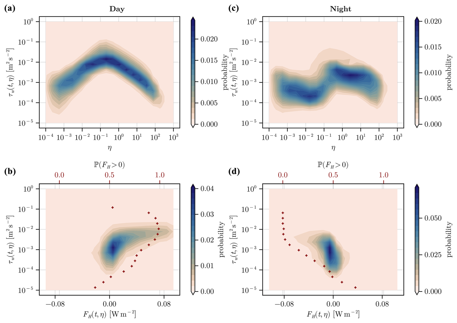
Figure 3 Probability densities of the amplitude of the vertical component of the Reynolds stress tensor τ_w(t,η) against normalised frequency η (a, c) and against the sensible heat flux F_H(t,η) (b, d), estimated from 10 to 19 June 2022 via kernel densities from 8 h data during daytime (a, b) and during night (c, d). Red crosses show the empirical probability function where sensible heat is positive $\left(\mathbb{P}\right(F_H>\mathrm{0})>\mathrm{0.5})$ or negative $\left(\mathbb{P}\right(F_H>\mathrm{0})<\mathrm{0.5})$ (upper x axis) vs. τ_w.

In the bottom row, we show with red crosses the empirical probability distribution of the sensible heat being positive or negative as a function of the amplitude of τ_w. We observe that an increase in the amplitude of τ_w corresponds to a higher empirical probability of heat exchange occurring (either positive or negative, depending on the stratification). The distribution of sensible heat is mainly positive during day, and the density covers mainly positive sensible heat when above τ_w ≃ 10⁻³ m² s⁻² (Fig. 3b). The distribution is mainly negative during night, and the density covers mainly negative sensible heat when above roughly τ_w ≃ 10⁻³ m² s⁻² (Fig. 3d). Choosing hence the noise threshold δ_τ = 10⁻³ m² s⁻² allows for clear extraction of the time–frequency regions characterising turbulent transport of heat during day and night.

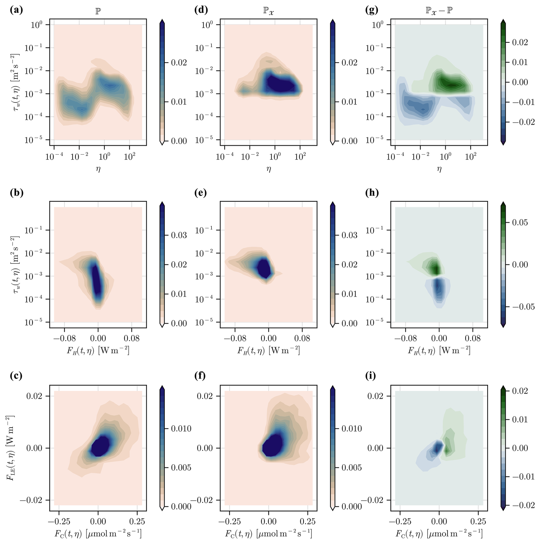
We present additional figures on the effect of applying the turbulence mask on time- and frequency-decomposed fluxes in Appendix A4, during daytime (Fig. A3) and nighttime (Fig. A4), with the additional densities of latent heat versus carbon fluxes. By looking at the differences in the probability densities of the data before and after applying the turbulence mask, we remark that the application of the turbulence mask (1) leads to the exclusion of large-scale structures with relatively high τ_w amplitude around η = 10⁻⁴, especially at night (Fig. A4g); (2) correctly preserves the turbulent exchange of heat during day and night (Fig. A4h, A3h); and (3) shows that carbon respiration, photosynthesis, and evapotranspiration processes are clearly visible in the estimates (Fig. A4i, A3i). At night in particular, the application of the turbulence mask removes negative latent heat fluxes and carbon uptake (Fig. A4i), which are considered noise and likely caused by large-scale structures (see Scanlon and Sahu, 2008, Fig. 3).

3.3 Results in different conditions

Figure 4 illustrates results of the methodology across 4 d, characterised by different conditions: 2 spring days in sunny (15 June 2022, Fig. 4a) and cloudy (1 May 2022, Fig. 4c) conditions and 2 winter days in sunny (12 February 2022, Fig. 4b) and cloudy conditions (26 January 2022, Fig. 4d). For each day, we compare the estimations of latent heat with our methodology (HRTM) against estimations in time and frequency space without a turbulence mask (HR), i.e. including large-scale contributions down to η ≃ $\mathrm{2}\times {\mathrm{10}}^{-\mathrm{4}}$, and against the standard at 30 min eddy-covariance estimations (EC30), which corresponds roughly to integrate the flux above η ≃ $\mathrm{5}\times {\mathrm{10}}^{-\mathrm{3}}$. The estimation without a turbulence mask (HR) is equivalent to cross-scalogram smoothing without an identification of turbulence in time–frequency space. The HR flux results are thus from integration over all frequencies without the first frequency band spanned by the low-pass filter (see Sect.2.4).

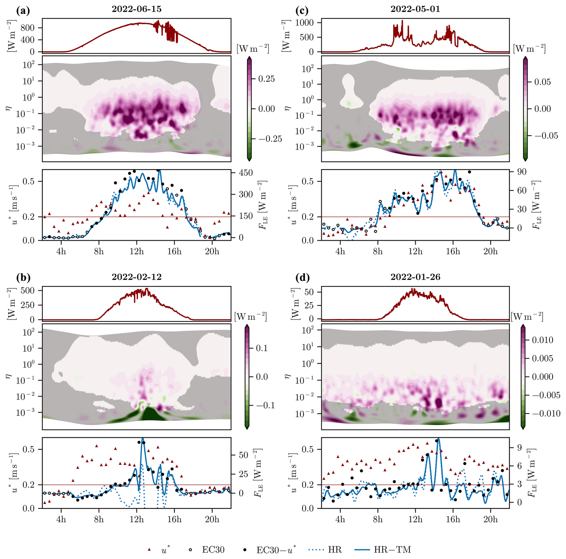
Figure 4 Estimation of latent heat flux on 4 selected days in different conditions: sunny conditions (a, b), cloudy conditions (c, d), during spring (a, c), and in winter (b, d). For each day, we show incoming shortwave radiation (top), time- and frequency-decomposed latent heat flux (middle), and flux estimates through time (bottom). Ten minute high-time-resolution fluxes are shown using the turbulence mask (solid line, HRTM) or integrating over all frequencies without mask (dotted line, HR). The standard eddy-covariance estimations over 30 min (EC30) are shown as circles. They are open symbols if they would be filtered out by a u^* threshold of 0.2 m s⁻¹. u^* (red triangles) is shown on the left axis of the bottom panels. Note that all y axes have different ranges to clearly show the differences between the fluxes on the different days.

The EC30 and HRTM estimations of the latent heat flux are roughly equivalent over the 4 selected days. However, the HR method can produce highly biased estimates such as on 12 February 2022 (Fig. 4b), with negative peaks in latent heat of about −150 W m⁻² during the day, or on 1 May 2022 (Fig. 4c), with negative fluxes around −15 W m⁻². Estimations from simple cross-scalogram smoothing HR hence cannot be used without proper filtering in time–frequency space. The proposed method of using a turbulence mask on top of cross-scalogram smoothing is one way to ensure that eddy fluxes are properly estimated and that the influence of external processes and noise are removed.

The friction velocity u^* is calculated using ${\left({\stackrel{\mathrm{‾}}{u^{\prime }{w}^{\prime }}}^{\mathrm{2}}+{\stackrel{\mathrm{‾}}{v^{\prime }{w}^{\prime }}}^{\mathrm{2}}\right)}^{\mathrm{1}/\mathrm{4}}$ with the standard eddy covariance for estimating the kinematic fluxes ($\stackrel{\mathrm{‾}}{u^{\prime }{w}^{\prime }}$ and $\stackrel{\mathrm{‾}}{v^{\prime }{w}^{\prime }}$). The friction velocity and the turbulence mask are overall in agreement; i.e. u^* is high when the turbulence mask covers large time–frequency regions with strong flux amplitude, and u^* is low when no time–frequency regions are covered or when it covers regions of very low flux amplitude. We remark some exceptions such as on day 15 June 2022 (Fig. 4a) during the afternoon when two half-hour estimates of EC30 would be flagged while the turbulence mask assesses that there is enough turbulence for a good flux estimation.

The dynamic of the incoming shortwave radiation signal is clearly reflected in HRTM. The effect of the passing of clouds at noon on 1 May 2022 (Fig. 4c) reduces the latent heat flux, followed by a slow increase in sunlight and latent heat from 12 to 16 h. Due to the high resolution of the proposed approach, fast dynamic processes in the turbulent fluxes can be observed. The relation between these turbulent fluxes and the sources and sinks of the ecosystem must be analysed separately.

3.4 Statistics over 8 h periods

We show in Fig. 5 statistics on the estimations of CO₂ fluxes over 8 h periods during day and night for 9 to 10 d periods in spring (10–19 June 2022) and winter (3–11 March 2022). We show the inter-decile range and the mean of the estimated fluxes from our method (HRTM) against the standard eddy-covariance approach (EC30).

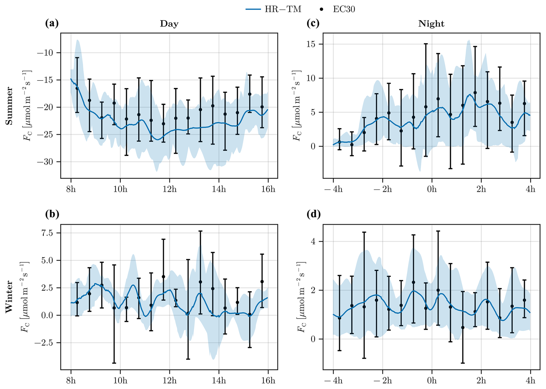
Figure 5 Daytime (a, b) and nighttime (c, d) CO₂ fluxes of consecutive days with high irradiance and no precipitations. (a, c) 10–19 June 2022; (b, d) 3–11 March 2022. The error bars on EC30 and the shaded areas of HR represent the 10th to 90th percentile range. Note that the y axes have different ranges to show differences between the flux estimates on the different days.

HRTM estimates are approximately in agreement with EC30 on average. Their spreads are of the same order of magnitude in summer but are larger for EC30 in winter during daytime (Fig. 5b). HRTM estimates show larger carbon uptake by +2 ± 1 $\mathrm{\mu }\mathrm{mol}{\mathrm{m}}^{-\mathrm{2}}{\mathrm{s}}^{-\mathrm{1}}$ during daytime in summer (Fig. 5a). This is explained by EC30 likely missing some carbon uptake below and around the scale η = 10⁻². During daytime in winter (Fig. 5b), both methods give weak and positive fluxes on average but sometimes also contain negative fluxes. Estimations of CO₂ fluxes at night are close between HRTM and EC30 in summer and winter (Fig. 5c–d). Fluxes should be positive at night. HRTM rarely shows negative fluxes at night, which is much more common in EC30 (Fig. 5c–d). The fixed averaging length of EC30, typically set to 30 min, is not well suited for capturing the turbulent exchange driven by mechanical shear at night. This interval is typically set for turbulent exchange under unstable stratification, whereas the turbulence spectra at night shift towards higher frequencies. As a result, nighttime EC30 estimates are corrupted in the normalised frequency range η = $\mathrm{5}\times {\mathrm{10}}^{-\mathrm{3}}$ to η = 10⁻¹, due to external processes that increase variability in the estimates, often leading to non-physical negative carbon fluxes during the night.

In Appendix A3, additional figures are presented for sensible and latent heat fluxes. For sensible heat fluxes (Fig. A2a), both the mean and the spread of EC30 and HRTM estimates are close. For latent heat fluxes (Fig. A2b), EC30 and HRTM estimates are approximately in agreement on average. HRTM estimates show smaller latent heat fluxes by −37 ± 7 W m⁻² during daytime summer (Fig. A2bA). Also, while latent heat fluxes should be positive, we remark that at night EC30 is more likely to produce negative estimates (Fig. A2bC–D).

3.5 Discussion

The proposed methodology introduces a novel framework for estimating eddy fluxes by leveraging time–frequency analysis, specifically through the use of cross-scalogram smoothing with generalised Morse wavelets. This approach addresses key limitations of the standard eddy-covariance method, particularly its fixed averaging time and the challenges associated with filtering perturbative scales under varying turbulence conditions. By decoupling the filtering of perturbative scales from flux calculations, our method enables a more adaptive and precise estimation of turbulent transport, resulting in a better assessment of fluxes across different environmental conditions.

The presented framework is a generalisation of the standard eddy-covariance approach, which employs more frequency bands to calculate fluxes and provides estimations continuously through time. One of the primary strengths is its ability to identify turbulent structures adaptively. Unlike the standard eddy-covariance approach, which relies on a fixed averaging time, the proposed framework dynamically adjusts to changing turbulence conditions. This adaptability is achieved through the use of a turbulence mask, which is derived from the vertical component of the Reynolds stress tensor. The mask effectively localises turbulent coherent structures in the time–frequency domain, allowing for a more accurate isolation of turbulent transport from noise and larger-scale processes. This adaptive identification ensures that the estimated fluxes are more representative of the actual turbulent exchange, even under varying stratification conditions, such as those observed during daytime buoyancy-driven turbulence and nighttime mechanical shear.

Another key advantage is the flexibility in adjusting the averaging time without compromising the filtering of perturbative scales. In the standard eddy-covariance method, reducing the averaging time to capture faster dynamics can lead to biases, as the filtering of perturbative scales becomes less effective. Our approach, however, allows for the averaging time to be adjusted independently of the filtering process. This flexibility is particularly valuable for studying ecosystem responses to rapid environmental changes.

At the FR-Hes site, the results demonstrate that the proposed method is consistent with the standard eddy-covariance approach, particularly during daytime with strong turbulence where the standard approach is known to perform well with good calibration of the averaging time. Moreover, the method shows better estimations of fluxes under weak turbulence in stable stratification, particularly during nighttime conditions where the fixed averaging time of the standard approach should be made shorter than during the day.

Despite these advantages, it is important to acknowledge the computational cost associated with our method. The current implementation requires approximately 10 min to process 24 h of fluxes (kinematic, CO₂, sensible heat, and latent heat fluxes) on a high-performance CPU, with a memory usage of around 16 GB of RAM. While this cost is reasonable, it highlights the need for further optimisation. Potential improvements include limiting the number of scales analysed and parallelising computations, which could significantly reduce the computational burden. These optimisations would make the method more practical for routine flux calculations while still preserving its adaptive and accurate estimation capabilities.

Estimations of eddy fluxes have been made above a forest ecosystem, and to relate these to ecosystem fluxes, an additional analysis of the coupling of turbulence below and above the canopy should be made. The present methodology does not assess this coupling, and another step is required for filtering the flux only when a strong coupling is present. By integrating τ_w along the frequencies with the turbulent mask found, it is possible to derive an alternative metric in time equivalent to u^* or σ_w. This would provide a summary metric of τ_w through time along with the fluxes, which could subsequently be used to study coupling or the representativeness of the turbulent fluxes. This development is out of the scope of this paper but is the subject of ongoing research.

The sensitivity of our methodology for flux estimation against wavelet parameters is not presented in this work. However, we have identified three important factors for the decomposition of fluxes into time and frequency coordinates: (1) the conservation of the global flux, which is guaranteed by the normalisation step (see Eqs. 12 and 17); (2) the frequency resolution of the decomposition (J and Q parameters of Sect. 2.3); and (3) time–frequency localisation of the wavelet used for the decomposition (β, γ). The normalisation (factor 1) guarantees that the fluxes obtained after integrating the time–frequency decomposition have meaningful physical interpretation. In particular, we do not have to estimate any wavelet-reconstruction factor empirically as encountered with continuous wavelet transforms (e.g. Schaller et al., 2017). This means that we can safely apply the proposed methodology for decomposing signals and estimate flux quantities. It is important to have a sufficient number of frequency bands to separate the turbulent scales from the larger scales; thus, a high-frequency resolution (factor 2) is needed, and J and Q are set to adequately high values. The time–frequency localisation of the wavelets also has an impact on how the information about the turbulent transport is scattered across the time–frequency plane (factor 3). The shape of the wavelet conditions the ability to localise events in time and frequency coordinates. Thus, we follow the recommendations of Lilly and Olhede (2012) for setting γ around 3 and β > 1. Values away from these parameters tend to create wavelets with poor localisation and hence risk producing poor time and frequency decompositions. These factors also have their importance in the decomposition of the advective term in the conservation equation (Eq. 8). In Appendix A5, an analysis of the influence of the decomposition parameters on the approximations of the advective term in Eq. (6) is presented.

The current framework enables adjusting the averaging time for estimating the flux of any scalar in HRTM without affecting the filtering of perturbative scales. A precise setting of a lower bound for the averaging time could be informed by analysing the correlation functions of velocities and scalars. For instance, Lenschow et al. (1994) suggested setting an averaging size larger than the integral timescale, estimated by assuming an exponential model for the auto-correlation function of velocity. More recent studies, based on the random sweeping hypothesis of Kraichnan (1964), have shown through theoretical development (Wilczek and Narita, 2012), controlled experiments (Poulain et al., 2006; He and Tong, 2011), and simulations (Wilczek et al., 2014) that the velocity auto-correlation function exhibits more complex behaviour in both space and time. Specifically, for small time delays, τ, the auto-correlation function behaves as a Gaussian in the term τkv₀, where k is the wavenumber, and v₀ represents the large-scale velocity fluctuations (sweeping velocity). This suggests a potential lower bound for the averaging window, σ_min = ${\left(k_{\min }{v}_{\mathrm{0}}\right)}^{-\mathrm{1}}$, where k_min is the lowest wavenumber below which no turbulence is assumed. However, determining the appropriate averaging window to connect eddy fluxes to ecosystem-scale fluxes is beyond the scope of this study and requires further investigation. This specific issue may be addressed through large-eddy simulations or direct numerical simulations.

The measurement acquisition systems (anemometer, gas analyser) have transfer functions that induce errors in the measurements. A theoretical inverse transfer function T_s can be applied to reduce flux errors (Aubinet et al., 2012, Sect. 4.1.3). This transfer function can be directly taken into account during the normalisation step of the filters. With T_s being the total transfer function of the acquisition system for the scalar s, the new normalisation function of Eq. (17) would become

$$\begin{array}{}\text{(21)}& G\left(\mathit{\nu }\right)=\sqrt{T_s\left(\mathit{\nu }\right)}\sqrt{{\left|\widehat{h}\left(\mathit{\nu }\right)\right|}^{\mathrm{2}}+\sum _{\mathrm{0}\le i\le L}{\left|\widehat{{\mathit{\psi }}_{a_i}}\left(\mathit{\nu }\right)\right|}^{\mathrm{2}}}.\end{array}$$

Flux corrections can also be applied afterwards by directly weighting in time–frequency coordinates the time- and frequency-decomposed fluxes.

4 Conclusions

In this paper, we presented a general framework for identifying turbulence and decomposing fluxes in the time–frequency domain, utilising generalised Morse wavelets. The effectiveness of this approach was demonstrated through its application at the FR-Hes site, where it was compared with the standard 30 min eddy-covariance method. Our framework addresses some of the difficulties mentioned regarding the use of wavelets by ensuring flux conservation and offering flexibility in parameterisation.

A key innovation of our method is the decoupling of perturbative scale filtering from flux calculations. This allows the averaging time to be adjusted without compromising the decomposition. The turbulence coherent structures are identified through a novel method based on the time–frequency analysis of the Reynolds tensor.

The flexibility to change the averaging time opens up new research perspectives, particularly the analysis of ecosystem responses to rapid environmental changes (less than 1 h). To support broader adoption and further development, we have made our method available as a Julia software package, TurbulenceFlux.jl, offering the community a tool for time–frequency flux estimation.

Appendix A

A1 Sufficient conditions on filters and averaging function for global flux conservation

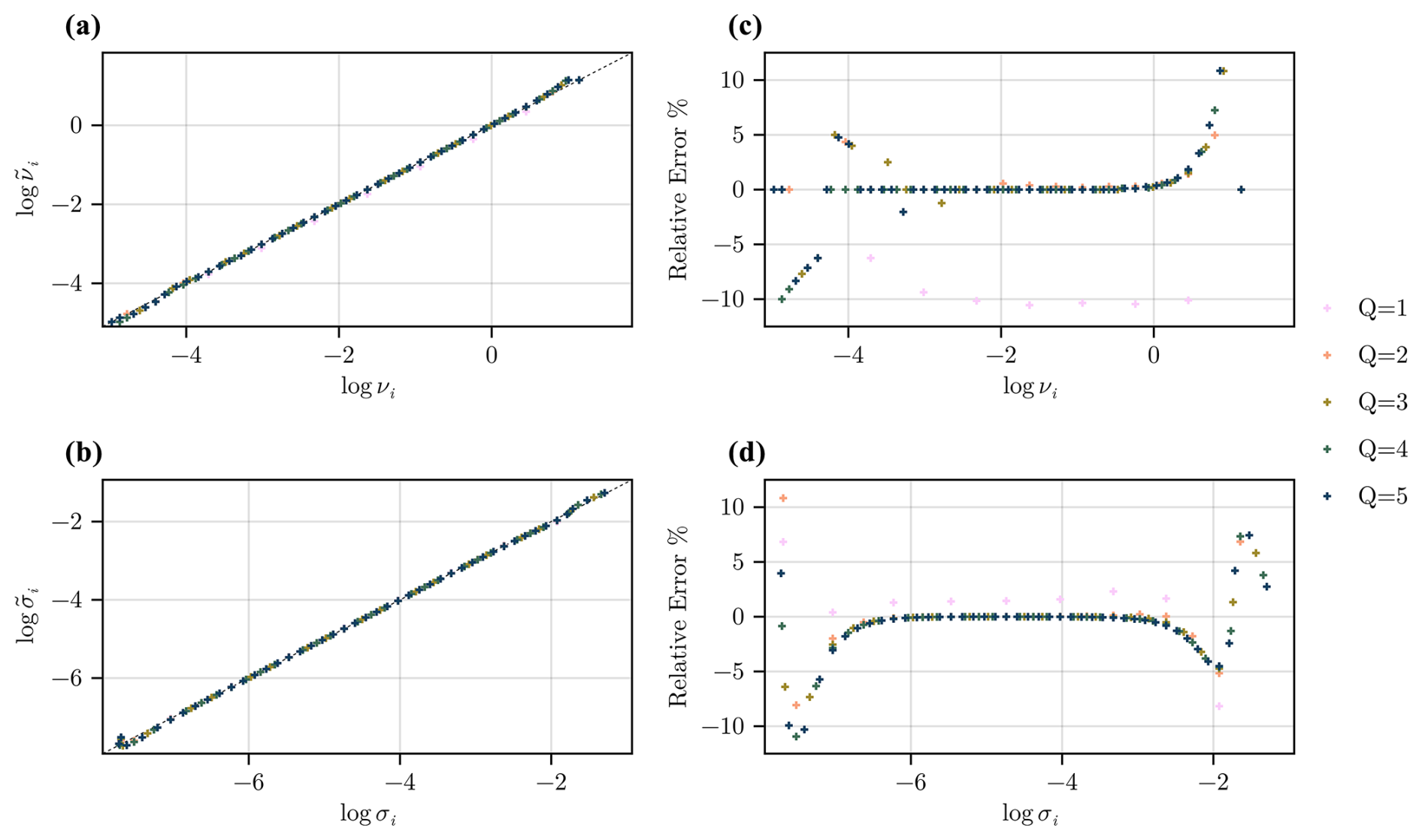
Figure A1 Effect of the self-dual normalisation (Eq. 17) on wavelet frequency peaks and time deviations. (a) Frequency peaks {ν_i}_i in log scale before (ν_i, x axis) and after (${\stackrel{\mathrm{̃}}{\mathit{\nu }}}_i$, y axis) normalisation. (c) Relative error of the frequency peaks after normalisation. (b, d) The same analysis but with time deviations.

We demonstrate here that the self-dual property of the filters (Condition 2.1) and the normalisation property of the averaging function (Condition 2.2) are sufficient conditions to preserve the global flux (Eq. 14). Assuming L filters are used for the decomposition, we get

$$\begin{array}{}\text{(A1)}& {\displaystyle }\begin{array}{l}\frac{\mathrm{1}}{T}\underset{\mathrm{0}}{\overset{T}{\int }}\sum _{l=\mathrm{1}}^L\left(w_l{s}_l\times \mathit{\varphi }\right)\left(u\right)\mathrm{d}u=\frac{\mathrm{1}}{T}\sum _{l=\mathrm{1}}^L\underset{\mathrm{0}}{\overset{T}{\int }}{w}_l\left(t\right)s_l\left(t\right)\mathrm{d}t,\\ \text{with Condition 2.2}\end{array}\text{(A2)}& {\displaystyle }=T\sum _{l=\mathrm{1}}^L\sum _p\widehat{w_l}\left(p\right)\widehat{s_l}(p{)}^{*},\end{array}$$

with ${\cdot }^{*}$ representing the complex conjugate operator and using Parseval's formula (see Mallat, 2009, Thm. 2.3):

$$\begin{array}{}\text{(A3)}& {\displaystyle }\begin{array}{l}=T\sum _{l=\mathrm{1}}^L\sum _p\widehat{w}\left(p\right)\widehat{s}(p{)}^{*}{\left|{\widehat{\mathit{\psi }}}_l\left(p\right)\right|}^{\mathrm{2}}=T\sum _p\widehat{w}(p\left)\widehat{s}\right(p{)}^{*},\\ \text{with Condition 2.1}\end{array}\text{(A4)}& {\displaystyle }={\displaystyle \frac{\mathrm{1}}{T}}\underset{\mathrm{0}}{\overset{T}{\int }}w\left(t\right)s\left(t\right)\mathrm{d}t=F_{\mathrm{s}}^T.\end{array}$$

A2 Impact of normalisation on the frame of wavelets

We analyse the impact of self-dual normalisation presented in Eq. (17) on an initially constructed frame of wavelets ${\left\{{\mathit{\psi }}_l\right\}}_l$ from which some properties are theoretically known such as the frequency peak.

We drop temporarily the $\widehat{\cdot }$ notation indicating that we are working with Fourier transforms, and we note ψ(ν) the Fourier transform of the wavelet ψ at frequency ν. With $\stackrel{\mathrm{̃}}{{\mathit{\psi }}_l}\left(\mathit{\nu }\right)={\mathit{\psi }}_l\left(\mathit{\nu }\right)/G\left(\mathit{\nu }\right)$, our set of wavelet filters with self-dual normalisation is $G=\sqrt{{\sum }_l{\left|{\mathit{\psi }}_l\right|}^{\mathrm{2}}}$. We do not take into account the low-pass filter here. The total derivative is given by

$$\begin{array}{}\text{(A5)}& d\stackrel{\mathrm{̃}}{{\mathit{\psi }}_l}={\displaystyle \frac{d{\mathit{\psi }}_l}{G}}\left(\mathrm{1}-{\left|{\displaystyle \frac{{\mathit{\psi }}_l}{G}}\right|}^{\mathrm{2}}\right)-\sum _{j\ne l}{\left|{\displaystyle \frac{{\mathit{\psi }}_j}{G}}\right|}^{\mathrm{2}}{\displaystyle \frac{d{\mathit{\psi }}_j}{G}}.\end{array}$$

Figure A2 Same as Fig. 5 but for sensible and latent heat fluxes.

Impact on frequency peaks. In order to study the impact of the normalisation, we analyse the derivative of $\stackrel{\mathrm{̃}}{{\mathit{\psi }}_l}$ against β. Let ψ_l = ${\mathit{\psi }}_{a_l}$ be a wavelet (here its Fourier transform) with frequency peak normalisation. We can show that

$$\begin{array}{}\text{(A6)}& {\displaystyle \frac{\partial {\mathit{\psi }}_{a_l}\left(\mathit{\nu }\right)}{\partial \mathit{\beta }}}={\mathit{\psi }}_{a_l}\left(\mathit{\nu }\right)\log {\displaystyle \frac{a_l\mathit{\nu }}{(\mathit{\beta }/\mathit{\gamma }{)}^{\mathrm{1}/\mathit{\gamma }}}}.\end{array}$$

At the frequency peak ${\mathit{\nu }}_l=\frac{\mathrm{1}}{a_l}(\mathit{\beta }/\mathit{\gamma }{)}^{\mathrm{1}/\mathit{\gamma }}$, we have $\frac{\partial {\mathit{\psi }}_{a_l}\left({\mathit{\nu }}_l\right)}{\partial \mathit{\beta }}=\mathrm{0}$.

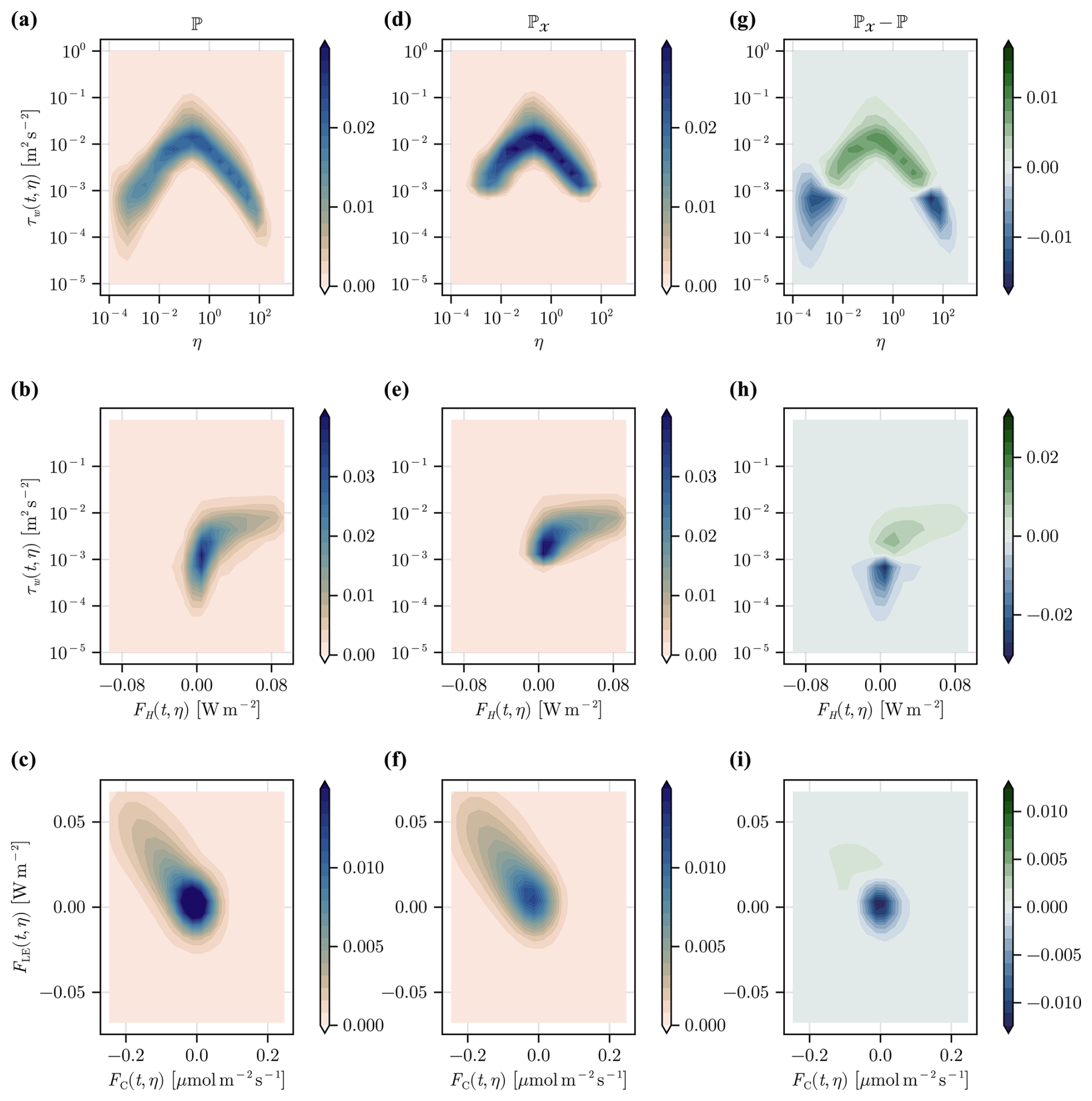
Figure A3 Effect of the application of the turbulence mask on the distributions of time- and frequency-decomposed fluxes during 8 h daytime periods from 10 to 19 June 2022. Probability densities of the fluxes without turbulence mask filtering (ℙ, a, b, c), with turbulence mask filtering (ℙ_𝒳, d, e, f), and their differences (ℙ_𝒳−ℙ, g, h, i), where negative values show where data have been removed by the turbulence mask filtering.

We check if the new set of filters keep the same frequency peaks by looking at the derivative of $\stackrel{\mathrm{̃}}{{\mathit{\psi }}_l}$ against β around the frequency peaks. With the notation ${\partial }_{\mathit{\beta }}\cdot =\frac{\partial \cdot }{\partial \mathit{\beta }}$, we get

$$\begin{array}{}\text{(A7)}& {\displaystyle }{\partial }_{\mathit{\beta }}\stackrel{\mathrm{̃}}{{\mathit{\psi }}_l}\left(\mathit{\nu }\right)={\displaystyle \frac{{\partial }_{\mathit{\beta }}{\mathit{\psi }}_l}{G}}\left(\mathrm{1}-{\left|{\displaystyle \frac{{\mathit{\psi }}_l}{G}}\right|}^{\mathrm{2}}\right)-\sum _{j\ne l}{\left|{\displaystyle \frac{{\mathit{\psi }}_j}{G}}\right|}^{\mathrm{2}}{\displaystyle \frac{{\partial }_{\mathit{\beta }}{\mathit{\psi }}_j}{G}}\text{(A8)}& {\displaystyle }={\displaystyle \frac{{\mathit{\psi }}_{a_l}\left(\mathit{\nu }\right)}{G}}\log (\mathit{\nu }/{\mathit{\nu }}_l)-\sum _j{\left|{\displaystyle \frac{{\mathit{\psi }}_{a_j}}{G}}\right|}^{\mathrm{3}}\log (\mathit{\nu }/{\mathit{\nu }}_j).\end{array}$$

At ν = ν_l = $\frac{\mathrm{1}}{a_l}(\mathit{\beta }/\mathit{\gamma }{)}^{\mathrm{1}/\mathit{\gamma }}=\frac{{\mathrm{2}}^{-l/Q}}{a_{\mathrm{0}}}(\mathit{\beta }/\mathit{\gamma }{)}^{\mathrm{1}/\mathit{\gamma }}$, with $a_l=a_{\mathrm{0}}{\mathrm{2}}^{l/Q}$,

$$\begin{array}{}\text{(A9)}& {\displaystyle }{\partial }_{\mathit{\beta }}\stackrel{\mathrm{̃}}{{\mathit{\psi }}_{a_l}}\left({\mathit{\nu }}_l\right)=-\sum _{j\ne i}{\left|{\displaystyle \frac{{\mathit{\psi }}_{a_j}}{G}}\left({\mathit{\nu }}_l\right)\right|}^{\mathrm{3}}\log ({\mathit{\nu }}_l/{\mathit{\nu }}_j)\text{(A10)}& {\displaystyle }=-{\displaystyle \frac{\log \mathrm{2}}{Q}}\sum _{j\ne l}{\left|{\displaystyle \frac{{\mathit{\psi }}_{a_j}}{G}}\left({\mathit{\nu }}_l\right)\right|}^{\mathrm{3}}(l-j).\end{array}$$

Around the lth wavelet, the effect of wavelet neighbours on the frequency localisation of the frequency peak compensate each other, and increasing the resolution Q decreases directly (through factor $\frac{\mathrm{1}}{Q}$) and indirectly (by increasing G in 1/G³) the impact of the normalisation. We expect, however, important modifications of the frequency peaks at the borders at high and low frequencies where fewer wavelets are present.

Figure A4 Same as Fig. A3 but during 8 h periods at night from 10 to 19 June 2022.

Impact on wavelet time deviation. The time deviation of a wavelet characterises how much it is concentrated in the time domain; thus, it is an effective measure of its scale. The time deviation of a wavelet ψ_ξ(t) (here in the time domain) can be computed using

$$\begin{array}{}\text{(A11)}& {\mathit{\sigma }}_l={\displaystyle \frac{\mathrm{1}}{T}}\sqrt{{\displaystyle \frac{{\int }_{-T/\mathrm{2}}^{T/\mathrm{2}}{\left|{\mathit{\psi }}_l\left(t\right)\right|}^{\mathrm{2}}{t}^{\mathrm{2}}\mathrm{d}t}{{\int }_{-T/\mathrm{2}}^{T//\mathrm{2}}{\left|{\mathit{\psi }}_l\left(t\right)\right|}^{\mathrm{2}}\mathrm{d}t}}},\end{array}$$

which is normalised by the maximum time support of wavelet T.

In Fig. A1, we show the impact of the normalisation on the frequency peaks or on the time deviations while increasing the resolution Q. Except at the borders, i.e. at low or high frequencies, the normalisation has limited effect on the frequency peaks location and on the time deviations if the resolution is high enough. It is then acceptable to use the theoretical frequency peaks of the original wavelets without normalisation to establish a proxy for measuring their scale (up to an unknown constant).

Figure A5 Relative squared error in the approximation of the averaged advective term for the multiple band decompositions as a function of the averaging length (a, d), the number of inter-octave bands (b, e), and the wavelet shape parameter β (c, f). The error is averaged across 10 d from 10 to 19 June 2022.

A3 Statistics of sensible and latent heat fluxes (see Fig. A2)

A4 Effect of the turbulence mask on fluxes distributions

In Figs. A3 and A4, we show the effect of the turbulence mask on the probability densities of fluxes in day and night conditions, respectively. We look in particular at the difference between the densities with and without the turbulence mask. We remark the following. (1) The application of the turbulence mask not just removes regions with low τ_w, i.e. below the threshold δ_τ = 10⁻³ m² s⁻², but the estimated time-varying spectral gap used to form the turbulence mask also helps in excluding high-amplitude τ_w regions at low frequencies around η = 10⁻⁴. This is particularly visible in Fig. A4 at nighttime conditions. This demonstrates that the proposed method reduces the influence of large-scale processes for estimating eddy fluxes which are located approximately in the frequency bands η = 10⁻² to η = 10² during day and in the bands η = 1 to η = 10² during night. These frequency bands are here mostly preserved by the application of the mask, except for the high end of the spectrum around η = 10² in daytime conditions where we transition from the inertial subrange occupied by the turbulent eddies to the dissipation range. (2) In day and night conditions, a weak and centred sensible heat flux is rejected while a strong positive (day) or negative (night) sensible heat flux is kept, which suggests that the turbulent exchange of heat by eddies is preserved. (3) During the day, weak and centred latent heat and carbon fluxes are removed through filtering while strong latent heat fluxes and strong carbon uptake, likely linked to evapotranspiration and photosynthesis, respectively, are preserved. During the night, strong negative latent heat and carbon fluxes are excluded by the turbulence mask while positive latent heat and carbon fluxes are preserved. This suggests that the turbulence identification correctly preserves the processes at play (respiration, photosynthesis, and evapotranspiration) in the turbulent exchange of water vapour and carbon between the forest and the atmosphere.

A5 Approximations in the decomposition of the advective term

We analyse here the viability of the approximations made in Eq. (6) for decomposing the advective term. We look at the relative squared error (RSE):

$$\begin{array}{}\text{(A12)}& \mathrm{RSE}\left(t\right)={\displaystyle \frac{{\left(\stackrel{\mathrm{̃}}{{\left[ws\right]}_{\mathit{\varphi }}}-{\left[ws\right]}_{\mathit{\varphi }}\right)}^{\mathrm{2}}\left(t\right)}{{\mathit{\sigma }}_{{\left[ws\right]}_{\mathit{\varphi }}}^{\mathrm{2}}}},\end{array}$$

where $\stackrel{\mathrm{̃}}{{\left[ws\right]}_{\mathit{\varphi }}}$ is an estimator of [ws]_ϕ, and ${\mathit{\sigma }}_{{\left[ws\right]}_{\mathit{\varphi }}}$ is the standard deviation of the averaged advective term over 24 h. We look at the viability of the “multiple band decomposition” estimator composed of wavelet filters:

$$\begin{array}{}\text{(A13)}& \stackrel{\mathrm{̃}}{{\left[ws\right]}_{\mathit{\varphi }}}=\sum _{l=\mathrm{1}}^L{\left[w_l{s}_l\right]}_{\mathit{\varphi }},\end{array}$$

with L filters as explained in Sect. 2.4.

Here, ϕ is a Gaussian window whose averaging length is controlled by its variance, and the target value is the averaged advective term [ws]_ϕ.

In Fig. A5, we show the influence of the averaging length, the number of inter-octave bands Q, and one of the wavelet shape parameters, β, in the approximation error. We study the advective term for vertical kinematic and sensible heat fluxes. We observe that the error is high with small averaging length and rapidly decreases with increasing averaging length, reaching ${\mathrm{10}}^{-\mathrm{3}}{\mathit{\sigma }}_{{\left[ws\right]}_{\mathit{\varphi }}}$ for vertical kinematic flux and ${\mathrm{10}}^{-\mathrm{2}}{\mathit{\sigma }}_{{\left[ws\right]}_{\mathit{\varphi }}}$ for sensible heat with 2 h averaging. The averaged advective term converges to the global flux with large averaging length, which is a quantity conserved by the multiple band decomposition. We note that decreasing the number of inter-octave bands, i.e. low Q, decreases slightly the error, because the number of inter-correlations between frequency bands being ignored is reduced. The shape parameter β also has an influence on the approximation. We note that decreasing its value reduces the error. This may be due to the shape of the overall turbulence co-spectrum which might be better captured with reasonably low β values.