A study of measurement scenarios for the future CO2M mission: avoidance of detector saturation and the impact on XCO₂ retrievals

The direct and indirect release of carbon dioxide (CO₂) by human activities into the atmosphere has been the main driver of anthropogenic climate change since the industrial revolution. The Paris Agreement from 2015 requires regular country-based reports of greenhouse gas emissions. Inverse modeling of observed concentrations of greenhouse gases is one important approach to verify reported emissions. The future constellation of Copernicus Anthropogenic CO₂ Monitoring (CO2M) satellites is dedicated to greenhouse gas measurements with high spectral and spatial resolution and wide coverage. The requirements for the performance of the instruments and retrieval algorithms for the column-averaged dry-air mole fraction (XCO₂) are stringent in order to identify, assess and monitor CO₂ emissions from space. In this study, we analyze the impact of avoiding detector saturation on the precision and spatial coverage of XCO₂. We use the Fast atmOspheric traCe gAs retrievaL (FOCAL) algorithm, which has been selected to be one of the operational greenhouse gas retrieval algorithms to be implemented within the CO2M ground segment. In order to avoid saturation, the number of read-outs per sampling time can be increased and the signals can be co-added on board, which we refer to as “temporal oversampling” in this study. We use a subsampled 1-year dataset of simulated radiances to define the temporal oversampling factors (OSFs) that are sufficient to avoid detector saturation and then apply the defined OSF combinations globally. We find that OSFs larger than 1 will lead to a significant decrease in the number of saturated observations, with some impact on the median XCO₂ precision, concluding that OSFs larger than 1 should be considered for the satellite mission. These results are based on simulated radiances. Consequently, the real impact on precision should be analyzed in more detail during the commissioning phase of the satellite.

1 Introduction

It is now well established that the direct and indirect release of carbon dioxide (CO₂) by human activities has been the most important cause of recent climate change since the industrial revolution (IPCC, 2023). Due to its long projected and irreversible impact on global warming on a timescale of a millennium (e.g., Archer et al., 2009; Solomon et al., 2009) and its sources from, e.g., fossil fuel combustion, reduction of CO₂ emissions is an internationally agreed environmental policy goal, as stated, e.g., in the Paris Agreement of 2015 (UNFCCC, 2015). This agreement requires that countries report their emissions on a regular basis. Atmospheric measurements of CO₂ concentrations, including, e.g., in situ surface observations and satellite-based remote sensing instruments, combined with inverse modeling to determine surface fluxes, offer a unique opportunity to verify and support these reported emissions.

Spaceborne total column CO₂ measurements have a long history, starting with those retrieved from the pioneering SCanning Imaging Absorption spectroMeter for Atmospheric CHartographY (SCIAMACHY) instrument (Burrows et al., 1995; Bovensmann et al., 1999; Buchwitz et al., 2005; Reuter et al., 2010; Schneising et al., 2011) and other satellites such as the Greenhouse gases Observing SATellite (GOSAT), GOSAT-2 (Kuze et al., 2009; Nakajima et al., 2012), the Orbiting Carbon Observatory (OCO) versions 2 and 3 (Crisp, 2015; Taylor et al., 2020), and TanSat (Liu et al., 2018).

The Copernicus Anthropogenic CO₂ Monitoring (CO2M) mission is a future constellation of three identical satellites in a near-polar sun-synchronous orbit with an Equator-crossing time at 11:30 LT in a descending node (Janssens-Maenhout et al., 2020; Sierk et al., 2021; Meijer et al., 2023). The first satellite is expected to be launched in 2027. The mission builds on the concepts of CarbonSat with extended instrumentation (Bovensmann et al., 2010; Velazco et al., 2011; Buchwitz et al., 2013; Pillai et al., 2016; Broquet et al., 2018). Its primary instrument is a push-broom imaging spectrometer (CO2I) measuring solar radiances reflected at the Earth's surface and scattered into the atmosphere in three spectral bands: (a) the near infrared (NIR; 747–773 nm), used to retrieve information about scattering properties and the atmospheric dry-air column density, aerosols and solar-induced fluorescence (SIF), (b) and two bands in the shortwave infrared (SWIR1, 1590–1675 nm, and SWIR2, 1990–2095 nm), used to derive information about atmospheric CO₂, CH₄, aerosols and water vapor. As a result, the satellites will enable the determination of the column-averaged dry-air mole fraction of atmospheric CO₂ and CH₄, called XCO₂ and XCH₄ hereafter, at a total spatial sample size of about 4 km² and a swath width of around 250 km. This resolution and swath width are a trade-off between detection of local sources and frequent global coverage, with some limitations, e.g., due to clouds covering the tropospheric signal. In addition to CO2I, the CO2M mission will enable the measurement of NO₂ content in the atmosphere with a spectrometer in the visible spectral range (NO2I), sharing the same slit, and provide information about clouds in the atmosphere with a cloud imager (CLIM) and about aerosols with a multi-angle polarimeter (MAP); see also Meijer et al. (2023) for an overview.

The potential for CO₂ emission verification with CO2M has been shown by studies using simulated radiances (e.g., Kuhlmann et al., 2020) and measurements of satellites already in operation (e.g., Reuter et al., 2019; Fuentes Andrade et al., 2024). Three retrieval algorithms are considered for the operational greenhouse gas product of CO2M, with differences especially in the treatment of light scattering in the retrievals: the Remote sensing of Trace gas and Aerosol Product (RemoTAP; Lu et al., 2022), the Flexible and Unified Spectral InversiON ALgorithm Platform (Fusional-P-UOL-FP) based on the algorithm described in Cogan et al. (2012), and the Fast atmOspheric traCe gAs retrievaL (FOCAL; Reuter et al., 2017a, b; Noël et al., 2021, 2022, 2024).

Quantifying anthropogenic CO₂ emissions from space is challenging because atmospheric signals resulting from these emissions are usually less than 1 % larger than the background (global ${\mathrm{XCO}}_{\mathrm{2},\mathrm{bg}}\approx \mathrm{419}\mathrm{ppm}$ in 2023, Copernicus Climate Change Service, 2024). In addition, the natural variability during the year is of a similar order of magnitude (e.g., Forkel et al., 2016). Therefore, the precision (0.7 ppm for CO2I) and accuracy requirements (0.5 ppm for CO2I) for the instrument calibration and retrieval algorithms are stringent (ESA, 2020). Consequently, all aspects influencing the precision of the retrieved XCO₂ have to be considered and analyzed carefully in order to meet these requirements. Precision values between 0.4 and 0.6 ppm could be inferred from several retrieval algorithms for CO2M using one read-out per integration time step (Lu et al., 2022; Reuter et al., 2025). Noël et al. (2024) showed first performance assessments of the FOCAL version for CO2M with simulated radiances. Here, we consider the effect of detector saturation and investigate the impact of reducing the detector exposure time in the nadir configuration where the instrument's zenith angle is close to zero in order to contribute to the planning of the commissioning phase of CO2M.

Detector saturation occurs when the number of photons collected by the detector is larger than the characteristic full-well capacity (FWC), e.g., due to a bright surface like a desert. Saturation of the detectors results in several negative impacts, which lead to errors in the CO₂ retrieval. At signal levels above the FWC, the detector typically exhibits strong non-linearity with a quickly fading response towards saturation (e.g., Staebell et al., 2021, for the airborne instrument MethaneAIR). In addition, saturation could affect subsequent measurements due to memory effects (Gaucel et al., 2023). Consequently, saturation-affected measurements have to be removed (Yoshida et al., 2011; Kataoka et al., 2017; Tian et al., 2018; Shi et al., 2021) and should generally be avoided. The GOSAT instrument has different gain modes to avoid detector saturation (Kataoka et al., 2017; Reuter et al., 2012; Taylor et al., 2022). In glint geometry over the ocean, where the satellite's field of view is shifted towards the sunglint spot, it has been found that saturation can affect measurements and can be avoided by looking near the glint spot but excluding it (Boesch et al., 2011; Eldering et al., 2012; Crisp et al., 2017). Saturation in general can also be avoided by reducing the exposure time of the detector, thereby not only increasing the maximum detectable radiance in that spectral band, but also impacting the retrieved XCO₂ precision (Nakajima et al., 2015; Grossmann et al., 2018; Staebell et al., 2021; Clavier et al., 2024). This is further discussed in Sect. 2.

The goal of this study is to define scenarios reducing the detector exposure time while maximizing coverage and minimizing the negative impact of saturation on XCO₂ precision. For this, we use simulated radiances calculated at the CO2M spatial samples with added noise corresponding to the respective detector setting. After defining detector saturation and its relation to the reduction in the exposure time in Sect. 2, we describe the simulated radiances used in this study (Sect. 3). As a next step, we define scenarios to determine the detector exposure time needed in each spectral band (see Sect. 4) and then apply these scenarios to simulated radiances and retrieve XCO₂ using the FOCAL algorithm (Sect. 5). The impact of the scenarios on the global XCO₂ precision is discussed in Sect. 6. Section 7 provides some concluding remarks.

2 Detector design, saturation, oversampling factor and signal-to-noise ratio

The design of CO2I/NO2I is comprised of four grating spectrometers sharing a common telescope, entrance slit and collimator, as described in Sierk et al. (2021). Here we briefly summarize the features that are relevant for the present study. The multi-band spectrometer operates according to the push-broom imaging principle: the entrance slit is projected onto the Earth's surface, defining the swath width in the across-track (ACT) direction. The CO2I/NO2I design features a slit composed of a number of rectangular optical fibers, which are aligned to form an array of apertures defining the spatial samples. The fiber core dimensions define the spatial sample size in the ACT direction (326 µm, corresponding to 1.8 km on Earth) and the instantaneous field of view (IFOV) in the along-track (ALT) direction (124 µm, corresponding to 814 m on Earth). The spatial sampling in the ALT direction is performed by the motion of the IFOV during the integration period t_int, in which signal is accumulated on the detectors.

The timing of the CO2I/NO2I instrument is driven by the requirements for (a) spatial sampling (≤4 km²) and (b) the signal-to-noise ratio (SNR) of the spectral radiance measurement; see also Appendix C for a more detailed discussion. The ACT spatial sampling distance is given by the design of the slit homogenizer (as well as detector size and optical magnification) and is fixed to 1.8 km. This allows for a maximum of ∼ 2.2 km spatial sampling distance in ALT. At the CO2M orbit, this amounts to a sampling time t_samp of about 308 ms. Shorter sampling periods will lead to a reduction in the SNR that is most probably non-compliant with the requirements, which is why the value of 308 ms is used in this study. A spatial sample, therefore, has an extent of about $\mathrm{1.8}\times \mathrm{2.2}\approx \mathrm{4}{\mathrm{km}}^{\mathrm{2}}$ (with small variation across the swath due to projection onto the Earth's surface). At any instant in time, the detector pixels sample the image spatially in the ACT direction and spectrally in the perpendicular direction. From the signal of the dispersed light (in electrons), integrated during the sampling period, radiance spectra are derived, one for each fiber comprising the entrance slit.

The number of electrons accumulated by a detector pixel sampling the wavelength λ, denoted as signal S(λ), depends on the ground scene and the properties of the spectrometer and can be as expressed as

$$\begin{array}{}\text{(1)}& S\left(\mathit{\lambda }\right)=L\left(\mathit{\lambda }\right)\cdot \mathit{\eta }\cdot \mathit{\tau }\cdot \mathrm{\Delta }\mathit{\lambda }\cdot \mathrm{QE}\left(\mathit{\lambda }\right)\cdot t_{\mathrm{int}},\end{array}$$

where L(λ) is the top-of-atmosphere spectral radiance, η the étendue of the instrument (product of the entrance pupil area and observation solid angle), τ the transmission of the optics, Δλ the spectral bandwidth (or sampling interval) of the pixel and QE the quantum efficiency of the detector. Here, t_int is the time during which light is accumulated within the sampling period. It has been decided to operate CO2I's SWIR detectors in “integration-then-read” mode in order to minimize bias effects from the detector's read-out electronics. In this mode, the signal of every acquired frame has to be completely read out before a new acquisition is started. During the read-out time t_RO of about 37 ms, the signal integration is paused. Accordingly, t_int as such is reduced by multiples of t_RO:

$$\begin{array}{}\text{(2)}& t_{\mathrm{int}}=t_{\mathrm{samp}}-\mathrm{OSF}\cdot t_{\mathrm{RO}}.\end{array}$$

The factor OSF denotes the temporal oversampling factor, which is the number of detector read-outs within the sampling time. An illustration of the integration times for different OSFs can be found in Fig. 1. Multiple read-outs (OSF>1) become necessary when the number of electrons accumulated during integration time exceeds the FWC of the detector pixels (called saturation hereafter). Note that the gaps in signal integration indicated by the white spaces in Fig. 1 are short with respect to the sampling time. They do not result in spatial undersampling as the IFOV in the ALT direction (approx. 800 m) is larger than the on-ground motion of the entrance slit image during the read-out time, which is about 200 m. An OSF larger than 1 increases the maximum radiance that can be measured by the detector, which is proportional to the time of each individual integration time (colored in Fig. 1).

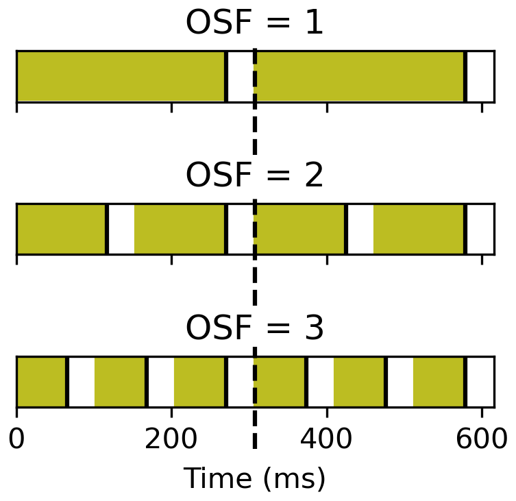
Figure 1 Illustration of the integration times (colored) for the oversampling factors that are foreseen for the detectors in the NIR and SWIR bands of CO2M. The white spaces are times for reading out the signal (about 37 ms). The end of the integration time is denoted by the solid black lines at the end of each rectangle. The dashed black line is the sampling period t_samp of 308 ms; see Eq. (2).

The detectors used for the NIR detector (Teledyne-E2V) and the two SWIR spectrometers of CO2I/NO2I (Lynred NGP) feature an FWC of approximately 61 000 and 650 000 electrons, respectively. If the signal acquired during integration time exceeds this limit, the respective detector pixel becomes saturated. Such pixels do not yield meaningful measurements, and tests showed that if saturation occurs, it usually does not happen only at one spectral detector pixel but for more than 3 % of the pixels with the largest signal. Therefore, it can be expected that a large fraction of the continuum range of the spectrum is affected by saturation so that the measurement is not useful for the retrieval and a radiance spectrum with saturated pixels has to be discarded. In order to avoid data loss, the detector can however be operated with OSF>1, meaning that more than one read-out cycle is performed within the sampling period of t_samp=308 ms (Fig. 1). The value of 308 ms was used to meet all demands within the mission requirements. Apart from data loss over bright ground scenes, the necessity for saturation avoidance by temporal oversampling (OSF>1) arises from the inherent effect of instrument stray light. Efficient correction of stray light from imperfect optical components (surface roughness and contamination), as well as parasitic reflections between them (“ghosts”), is mandatory to achieve compliance with the stringent radiometric requirements of the CO2M mission. Stray-light correction algorithms require accurate knowledge of the signal distribution across the focal plane, which is derived from the measured signal image. In the presence of signal saturation, and hence invalid radiation measurements, such correction becomes inaccurate, if not infeasible, since the largest stray-light contribution from the brightest signals cannot be reconstructed. For the reasons outlined above, the CO2I/NO2I spectrometer is likely to be operated with temporal oversampling, leading to signal loss according to Eq. (2). In the main part of this study, we neglect the effect of saturation on neighboring spatial samples in the swath and memory effects and remove spatial samples in the case of saturation in their spectrum.

A major drawback of oversampling is the loss of radiometric signal from the total read-out time OSF⋅t_RO, which decreases the SNR because the read-out noise increases with multiple read-outs. In order to quantify the impact of oversampling on the SNR, we further develop Eq. (1) to obtain an expression for the SNR of the measured radiances. The shot noise of the measurement, given by the square root of the signal S(λ), combines with the signal-independent components of the detection as

$$\begin{array}{}\text{(3)}& N_{\mathrm{total}}=\sqrt{S\left(\mathit{\lambda }\right)+(I_{\mathrm{dark}}+I_{\mathrm{Tb}})\cdot t_{\mathrm{int}}+(N_{\mathrm{RO}}^{\mathrm{2}}+N_{\mathrm{AD}}^{\mathrm{2}}+N_{\mathrm{VC}}^{\mathrm{2}})\cdot \mathrm{OSF}},\end{array}$$

where I_dark is the dark current of the detector, I_Tb the shot noise from background thermal emission, N_RO its read-out noise, N_AD the digitization noise and N_VC the video chain noise. The SNR can then be expressed as

$$\begin{array}{}\text{(4)}& \mathrm{SNR}={\displaystyle \frac{A\cdot L}{\sqrt{A\cdot L+B}}},\end{array}$$

in which the contributing noise sources are grouped into components scaling with the radiance L(λ) and read as

$$\begin{array}{}\text{(5)}& A=\mathit{\eta }\cdot \mathit{\tau }\cdot \mathrm{\Delta }\mathit{\lambda }\cdot \mathrm{QE}\left(\mathit{\lambda }\right)\cdot \left[t_{\mathrm{samp}}-(\mathrm{OSF}\cdot t_{\mathrm{RO}})\right]\end{array}$$

and signal-independent parameters determined by the detector and read-out electronics

$$\begin{array}{}\text{(6)}& B=(I_{\mathrm{dark}}+I_{\mathrm{Tb}})\cdot \left[t_{\mathrm{samp}}-(\mathrm{OSF}\cdot t_{\mathrm{RO}})\right]+(N_{\mathrm{RO}}^{\mathrm{2}}+N_{\mathrm{AD}}^{\mathrm{2}}+N_{\mathrm{VC}}^{\mathrm{2}})\cdot \mathrm{OSF}.\end{array}$$

As can be seen, both the numerator and the denominator in Eq. (4) are affected when the oversampling factor is increased: the signal is decreased by the multiple read-out times, in which no signal electrons are integrated, and the total noise is increased as more read-out noise is accumulated. Both effects reduce the SNR of the measured radiance for OSF>1.

In order to apply the different OSF scenarios to the radiances, we use A and B parameters provided to us by ESA (ESA, private communication, 2023) to compute the SNR in the data using Eq. (4). In the files, these parameters are given for an edge spatial sample and a center spatial sample at discrete integer wavelengths so that they have to be interpolated to all detector pixels. We used linear interpolation in both wavelength and across-track dimensions. The A and B parameters depend on the number of read-outs and thus on the OSF used so that the SNR is OSF-specific at each wavelength.

Optimization of in-flight operation calls for avoidance of saturation on the one hand, while maintaining the largest possible SNR of the measured radiance spectra on the other hand. This optimization requires a careful analysis of the expected radiance levels and their variation, based on the realistic simulation of ground scenes, which is the topic of this study.

3 Radiance spectra simulated with SCIATRAN

We base our investigations on simulated radiances at the CO2M spatial samples, which we use as input for the retrievals. With simulated radiances, we have exact control over the noise that is added to the radiances so that the impact of increasing the OSF can be separated from other instrumental effects. The same 1-year subset radiances, simulated with the SCIATRAN radiative transfer model, are used as described by Noël et al. (2024). Here, we provide a brief summary of the dataset.

For this dataset, eight ACT spatial samples (approximately every 15th) and every 20th ALT spatial sample with solar zenith angles (SZAs) smaller than 80^∘ (consistent with ESA, 2020) were selected using CO2M orbit data of 1 year provided by EUMETSAT to simulate nadir radiances over land at these CO2M spatial samples with SCIATRAN (Rozanov et al., 2017). The subset is chosen to reduce computation time while keeping an annual dataset and representatively sampling the geophysical conditions. The SCIATRAN radiative transfer model can be used to simulate radiative transfer through the Earth's atmosphere, including multiple scattering, in a wide range of wavelengths. For the generation of the dataset for this study, input pressure, temperature, clouds and water vapor profiles have been taken from the ECMWF re-analysis version 5 (ERA5; Hersbach et al., 2020) and other trace gas profiles, and input parameters for the simulation of aerosols are taken from the Copernicus Atmosphere Monitoring Service (CAMS; Inness et al., 2019) re-analysis data, both from the reference year 2015. The surface reflectivity needed to calculate the radiances has been derived using satellite measurements of the Moderate Resolution Imaging Spectroradiometer (MODIS). The simulation of solar chlorophyll fluorescence is based on Rascher et al. (2009). The simulations are restricted to scenes over land in the nadir mode of CO2M. Further details can be found in Noël et al. (2024).

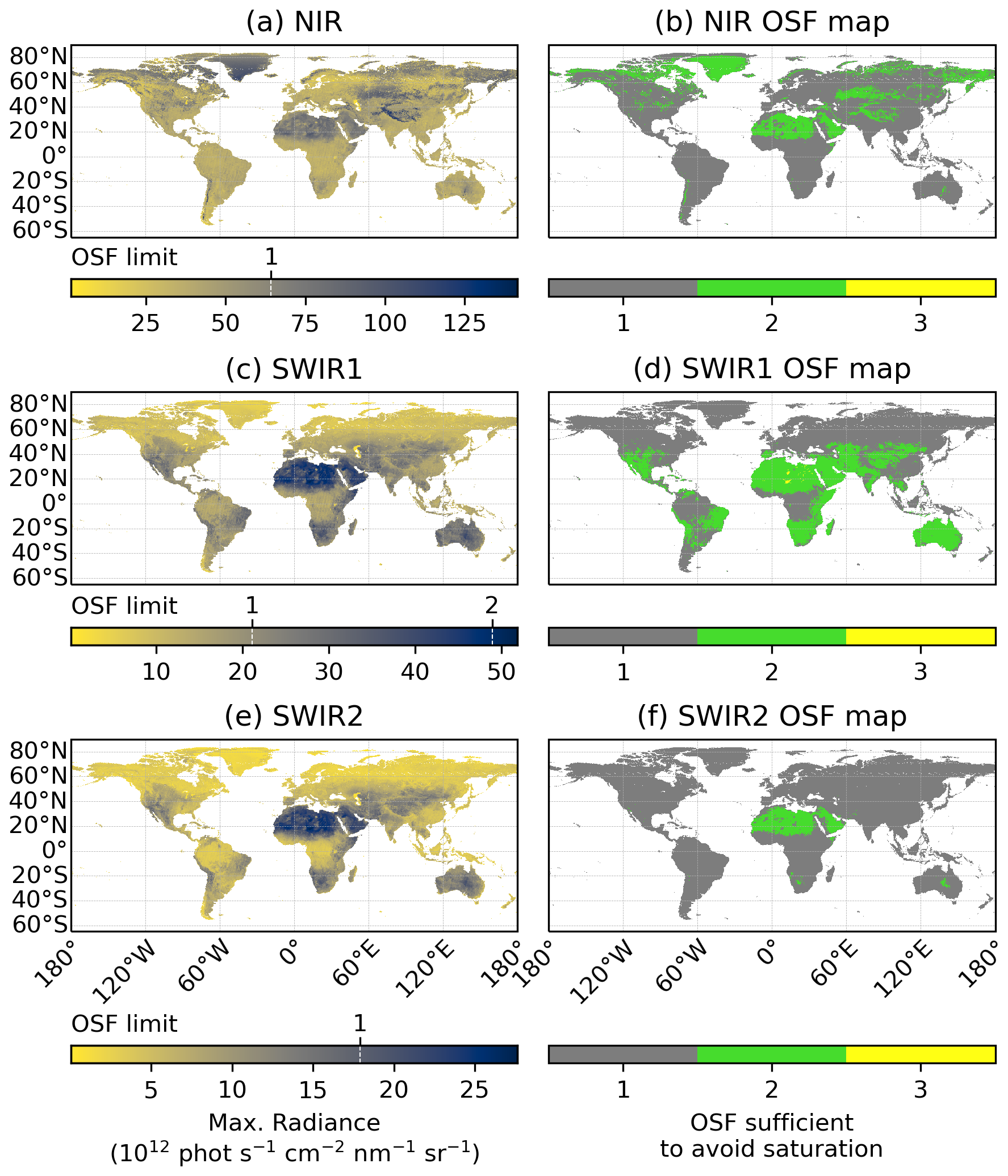
Figure 2 (a, c, e) Spectral and temporal maximum radiance in the simulated 1-year subset nadir radiances, binned to a 0.4×0.4° latitude–longitude grid. Clouds are removed for this analysis. The radiance limits corresponding to the OSFs in each wavelength band are illustrated by the dashed white lines in the color scales of the panels. (b, d, f) OSF needed in order to avoid saturation for the maximum radiances. The rows show the wavelength bands of CO2I: (a, b) NIR, (c, d) SWIR1 and (e, f) SWIR2. The simulated radiances are for nadir over land only. Therefore, the ocean is masked by the white color.

4 Defining scenarios that avoid detector saturation

The goal of this section is to determine the maximum radiance in each spectral band and compare it with the OSF-specific saturation limit in order to estimate the OSF needed to avoid saturation. While different OSFs could be used along one orbit, switching would make mission operations more complex and may lead to other challenges, such as OSF-dependent calibration (cf., Kataoka et al., 2017). Here, we investigate whether it is possible to use constant-OSF settings all over the globe.

The left column of Fig. 2 shows the spectral and temporal maximum radiance occurring during the 1-year dataset of simulated radiances. They are binned to a 0.4×0.4° grid, which corresponds roughly to the distance of every 15th spatial sample of CO2I/NO2I on the Earth's surface. As expected due to the solar irradiance spectrum, radiances are larger in the NIR bands than in the SWIR bands. The largest maximum radiances are simulated over desert regions, like the Sahara and the Australian deserts, especially in the SWIR bands, which are sensitive to different surface types (e.g., Fasnacht et al., 2019; Manakkakudy et al., 2023; Santamaría-López et al., 2024). Increases also occur over tropical rain forests due to the red edge of plants (e.g., Ge et al., 2019; Zeng et al., 2021). The ice-covered surface of Greenland shows increases in NIR bands and small values in SWIR bands.

The color scales in Fig. 2 also include the radiance limits for the OSFs in each band. The global maximum radiances in NIR and SWIR1 correspond to values exceeding the limit of saturation for OSF 1, indicating that OSF>1 might be needed to avoid saturation. The right column of Fig. 2 shows which OSF is sufficient in each grid box.

The limit for OSF 1 is exceeded over most parts of the land surface in the NIR band. In SWIR1, the latitude regions roughly between 30° N and 30° S, which include tropical forests and deserts, also exceed the saturation limit for OSF 1. The only region where an OSF of 3 is needed in the SWIR1 band is in the middle of the Sahara, where no significant anthropogenic sources of greenhouse gases exist. Therefore, OSFs 1 and 2 are the dominant OSFs that are sufficient for SWIR1. In SWIR2, only some of the deserts show exceedance of the limit for OSF 1, where OSF=2 would then be necessary to avoid saturation.

Table 1 Fraction of cloud-free spatial samples (in %) for which the radiance is between the saturation limits of OSF and OSF minus 1 in the 1-year dataset of simulated radiances.

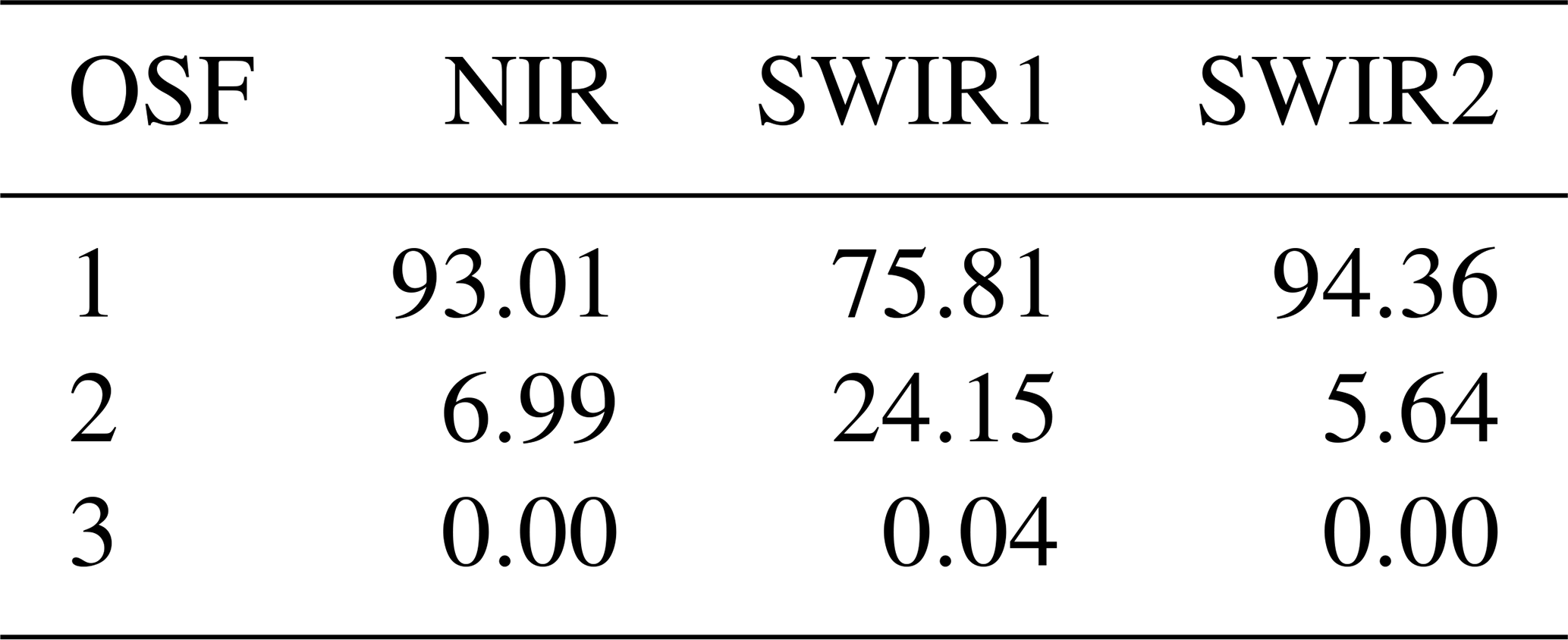
Table 1 shows the global fraction of spatial samples in the 1-year subset dataset where the shown OSF is needed to avoid saturation. As can be seen, about 7 % of all spatial samples within the simulated year exceed the threshold for OSF 1 in the NIR band. Although some spatial samples showed exceedance of the threshold for OSF=2 in the NIR band (Fig. 2), the actual fraction in the whole 1-year dataset is negligible. In the SWIR1 band, about 24 % of all spatial samples require OSF=2. The locations requiring an OSF of three (yellow in panel d of Fig. 2) correspond only to a minor fraction of 0.04 %. As expected from the previous analysis, the fraction for an OSF of two is smaller for SWIR2 than for SWIR1, with a value smaller than 6 %.

Table 2 Oversampling factor (OSF) scenarios for the spectral bands of CO2M with their notation in this study. These OSFs are assumed to be applied globally in this study; see the text for details.

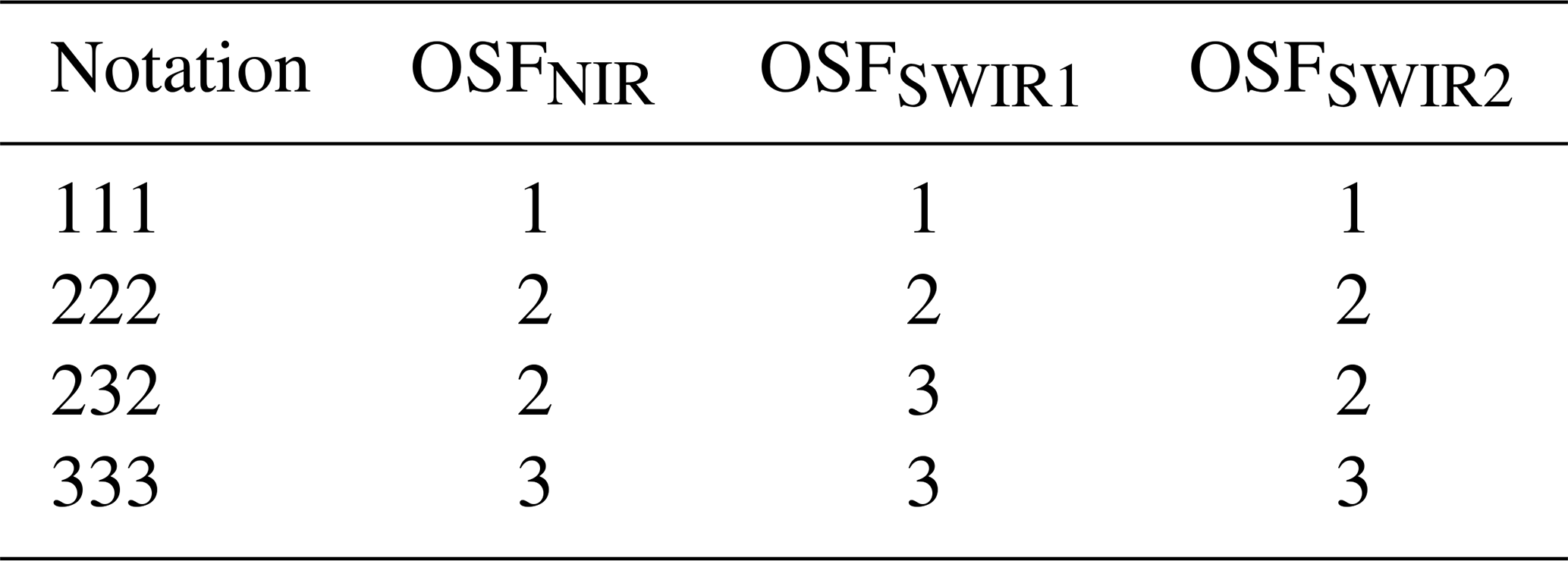
Therefore, a significant fraction of spatial samples is affected by saturation, with OSF=1 in all bands so that OSFs larger than 1 should be further investigated, which is the subject of this study. As the main fraction of saturated spatial samples is located over regions that are not known for large-emission CO₂ sources, like over deserts and snow, we regard the OSF scenario OSF=1 in all wavelength channels not only as a reference but also as one of the likely scenarios for CO2M. In addition, scenarios with OSF=2 in all channels are considered in this study. As we use only a sub-sampled dataset for the global analysis, we also add an OSF scenario with OSFs of 2 (NIR), 3 (SWIR1) and 2 (SWIR2) and a scenario with an OSF of 3 in all bands in case the missing spatial samples show larger radiances. The scenarios are summarized in Table 2 and denoted as OSFs 111, 222, 232 and 333, respectively.

5 The FOCAL greenhouse gas retrieval algorithm

In this study, we use the updated version 1.1 of FOCAL-CO2M, which is similar to the version used by Noël et al. (2024), with minor updates of coding optimizations. Therefore, we provide a brief summary of FOCAL here, with further details to be found in Noël et al. (2024) and references therein.

FOCAL is a radiative transfer and trace gas retrieval code that approximates scattering in the atmosphere by a single-scattering layer whose height, optical thickness and Ångström exponent are retrieved as part of the algorithm using optimal estimation. This approximation leads to an analytic expression for the calculation of scattering (Reuter et al., 2017b), making FOCAL a fast algorithm for the inversion of greenhouse gas concentrations from spectral measurements in the NIR and SWIR. FOCAL has been successfully applied to many satellites measuring greenhouse gases, such as OCO-2 (Reuter et al., 2017a, b), GOSAT and GOSAT-2 (Noël et al., 2021, 2022), and is one of the three operational algorithms that will be used to retrieve greenhouse gases from the future CO2M mission.

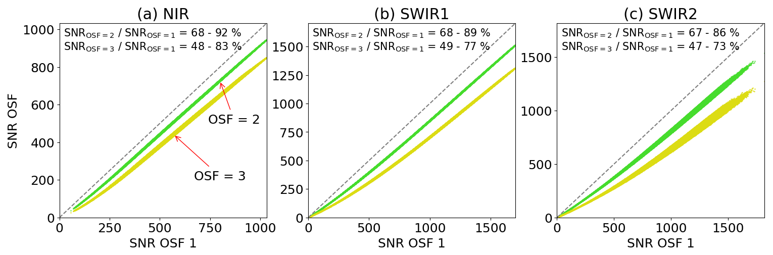
Figure 3 Signal-to-noise ratios compared to an OSF of one in (a) the NIR, (b) the SWIR1 and (c) the SWIR2 bands. The dashed black line illustrates the one-to-one line. In addition, the minimum and maximum of the ratio between the SNR to SNR for OSF=1 are labeled in each panel for each OSF.

The FOCAL algorithm comprises pre-processing (i.e., filtering of measurements with bad quality and difficult scenes such as high SZAs), inversion and forward modeling (i.e., optimal estimation with an iterative approach starting with a priori knowledge), and post-processing (i.e., convergence, variance filtering and bias correction). The setup of these steps here is similar to that used by Noël et al. (2024), which is why we refer to this publication for the details and describe the adaptions made for this study here.

As the noise model and the post-processing are specific to the setup of the instrument, e.g., the OSF, and we assume the application of one OSF scenario all over the globe, we use different noise models and post-processing for each OSF scenario. The post-processing uses a variance minimization process and filters data that have the largest impact on the scatter of the difference from the truth so that, on average, the differences from the truth are minimized. This means that variables and their limits to minimize the variance differ between the OSF scenarios, while the total fraction of measurements that are removed is kept constant, which makes the OSF scenarios comparable to each other. Note that post-processing is based on 10 % of the whole year's data. The setup of the noise model and the post-processing can be found in Appendix A.

In this study, we apply FOCAL-CO2M version 1.1 to 1 year of simulated subset nadir radiances over land, filtered for clouds, an SZA larger than 75° and saturation, and retrieve XCO₂ using the OSF scenarios of Table 2. The impact on XCO₂ is discussed in the following section.

We use the retrieval's random noise error arising from the different components discussed in Sect. 2 to investigate the impact on the XCO₂ precision. In addition, we analyze the retrieval's smoothing error, which arises from the smoothing of the state connected to the averaging kernels (Rodgers, 2000), in combination with the noise error, to provide insights into the impact on the overall noise error. The remaining systematic errors after post-processing due to the different OSF settings should be small because the post-processing is calculated individually for each OSF scenario and is analyzed in terms of the overall standard deviations of the retrieval residuals.

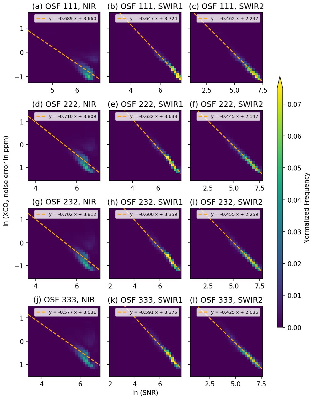
Figure 4 Logarithm of the continuum SNR versus logarithm of the FOCAL XCO₂ a posteriori noise error for all combinations of OSF scenarios and wavelength bands. The dashed orange lines show linear regressions for each panel, with its parameters in the legend. Note the different values on the x axes of each panel.

6 Impact of increasing the OSF

6.1 Impact on SNR

We first analyze how the SNR of the continuum radiance is affected by an increased OSF. Figure 3 shows the reduction in the SNR compared to OSF=1 for the three spectral bands. While the maximum SNR for OSF=1 is about 1000 in the NIR band and 1600 in the SWIR band, it is smaller for larger OSFs. For large SNRs, i.e., large radiances, A dominates Eq. (4), leading to a constant slope in all cases. The non-linear part corresponding to B leads to changes in the slope at the lower end of SNRs so that all lines converge to the origin. Ratios of SNR to OSF 1 are printed for each spectral band and are between 67 % and 92 % for OSF=2 and between 47 % and 83 % for OSF=3; see Fig. 3.

In the next step, we investigate the impact of the SNR changes, made in the previous analysis, on the retrieved a posteriori noise of FOCAL. This could be used in the future to estimate the XCO₂ precision with the knowledge of the SNR change. In the easiest case, relative changes in the SNR (Φ) are proportional to relative changes in the a posteriori noise error (N), which can be written as

$$\begin{array}{}\text{(7)}& {\displaystyle \frac{\mathrm{d}N}{N}}=C{\displaystyle \frac{\mathrm{d}\mathrm{\Phi }}{\mathrm{\Phi }}},\end{array}$$

where C is a constant translating SNR changes to changes in XCO₂ a posteriori noise, i.e., precision. This assumption is tested in this section. Integrating Eq. (7) yields

$$\begin{array}{}\text{(8)}& \ln N=C\cdot \ln \left(\mathrm{\Phi }\right)+k,\end{array}$$

where k is an integration constant, and the knowledge that N and Φ are positive numbers has been applied.

Equation (8) describes a linear relationship between N and Φ in a double-logarithmic space. It has been tested for all scenarios and bands, which are shown in Fig. 4. This figure shows histograms of binned logarithmic SNR and a posteriori noise error values with linear regressions as dashed lines and formulas in the respective legends. The assumption of linearity does not apply to the NIR band, as some high SNR values also have a large noise error because radiances in the NIR band are less sensitive to changes in CO₂ (only indirectly due to the dependence of the retrieved XCO₂ on atmospheric scattering and on the air column or surface pressure) compared to the other bands. On the other hand, there is a clear linear relationship in the two SWIR bands. While the slopes of the regression lines differ among the OSF scenarios, the negative values are the largest in the NIR (average −0.69), smaller in SWIR1 (average −0.62), and the smallest in SWIR2 (average −0.45). The smaller slope in SWIR2 compared to SWIR1 can probably be explained by the different numbers of spectral detector pixels in the CO₂ absorption region within the FOCAL fit windows: about 473 in SWIR1 and 770 in SWIR2, which makes single noisy measurements less sensitive to changes in XCO₂ in SWIR2. In addition, the sensitivity of the absorption lines to CO₂ changes is different between SWIR1 and SWIR2.

In summary, the SWIR2 band is less sensitive to changes in the SNR than SWIR1, where the double-logarithmic linear relationship could be confirmed. Apart from values with a high SNR and large noise, for which the assumption of linearity does not hold, the slope in the NIR band is similar to that in the SWIR1 band, suggesting that the NIR band is of similar importance for the retrieval of XCO₂.

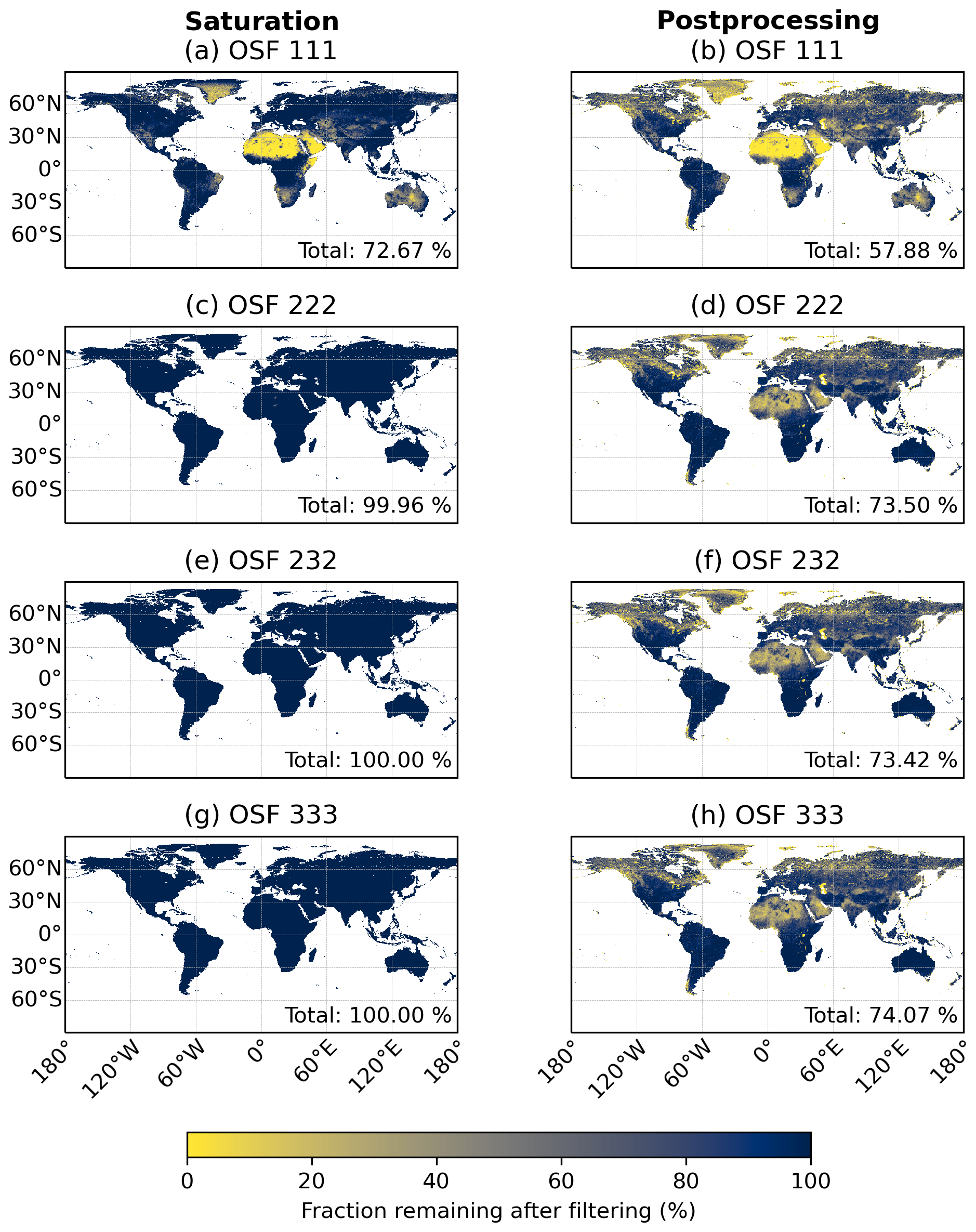
Figure 5 Throughput of the saturation filter during pre-processing (left column) and after post-processing (right column). The data are binned to a 0.4×0.4° latitude–longitude grid based on the CO2M spatial sample center coordinates. Note that the saturation filter is applied as the last filter, and 100 % means the data after filtering for SZA >75° and cloud fraction>0.2. The global fraction of remaining data is labeled “Total” in the panels. The filters applied during post-processing can be found in Table A1 of Appendix A.

6.2 Impact on spatial coverage

As discussed in Sect. 2, spectra including saturated measurements have to be discarded, which reduces the spatial coverage on Earth. In order to analyze the impact of filtering on saturation, the simulated radiances are binned to a 0.4×0.4° latitude–longitude grid, and the fraction of remaining data is shown in the first column of Fig. 5. As discussed above, the desert regions have large reflectances that will lead to saturation for all measurements in OSF 111 (panel a), e.g., over the Saharan region, the Arabian Peninsula and the deserts in Australia. Note that important emissions from the oil and gas industry on the Arabian Peninsula would have to be filtered out when using OSF 111. In addition, surfaces covered by ice, such as Greenland and the Himalayas, are filtered out as a result of saturation using OSF 111. In total, a fraction of 72.7 % remains globally when adding an additional pre-processing filter for saturation in OSF 111. Because of possible stray-light effects, we also did the analysis by removing whole swaths instead of single spatial samples, which can be found in Appendix B, and in which a fraction of 47.3 % remains after filtering for saturation.

As expected from the analysis in Sect. 4, increasing the OSF to values larger than 1 leads to better coverage. For instance, with OSF 222 (panel c), saturation only occurs at localized spots in the Sahara, leading to an overall remaining fraction of data larger than 99 %. For the scenarios with larger OSFs (232 and 333), 100 % of the values remain; i.e., no saturation or saturation in the sub-percent range is simulated in these cases. On the other hand, the majority of locations affected by saturation are in regions where no significant emission sources exist so that OSF 111 could still be sufficient for the goal of estimating localized emission sources.

Another aspect is post-processing, which filters parts of the data independently of saturation, and the fraction of data remaining after the saturation filter and post-processing is shown in the second column of Fig. 5. The filters applied during post-processing depend on the scenario and can be found in Table A1 of Appendix A. While the post-processing filters part of the data over the Sahara and the Arabian Peninsula for OSF>1 as well, data are additionally lost at high latitudes. The patterns are similar for all OSF scenarios. In total, about 58 % are left for OSF 111 and about 73 % for the other scenarios.

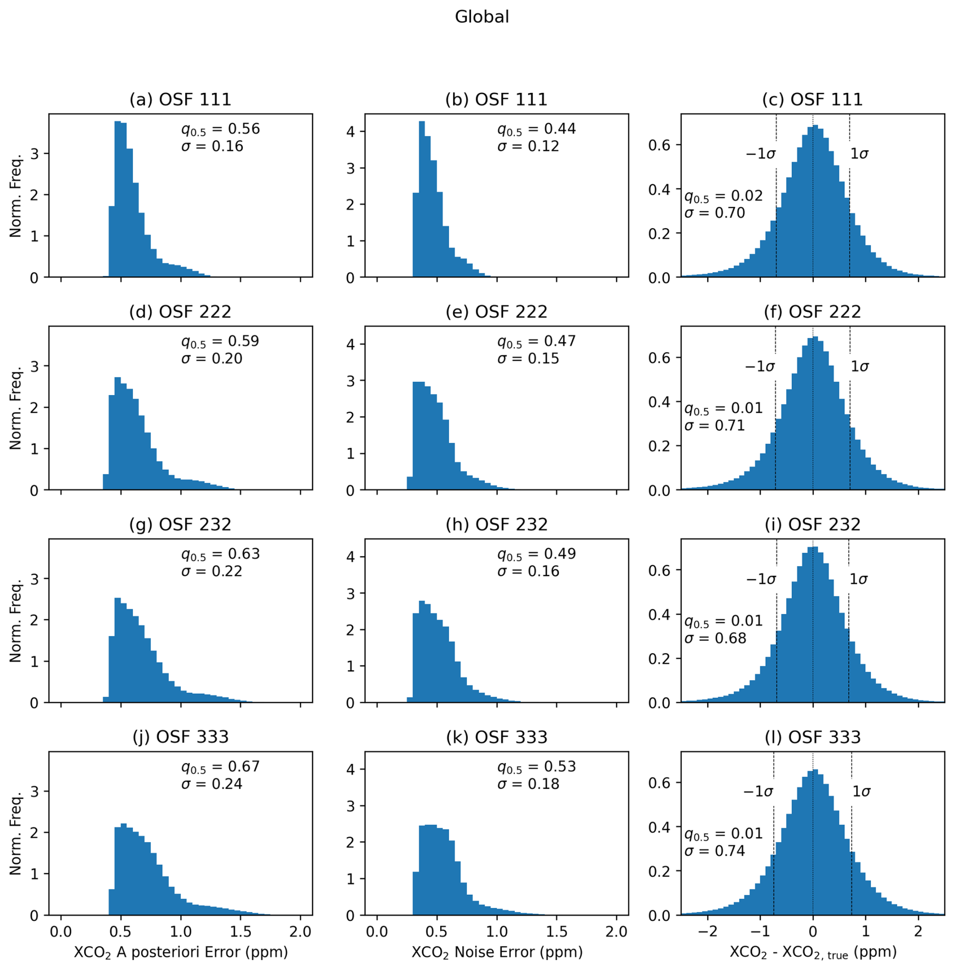
Figure 6 Histograms of the global distribution of the a posteriori XCO₂ retrieval error (first column), the a posteriori XCO₂ noise error (second column), and the differences between FOCAL XCO₂ after post-processing and the true XCO₂ (third column) for the whole year of simulated subset radiances. The rows show OSFs 111, 222, 232 and 333, respectively. The median (q_0.5) and standard deviation (σ) of the distributions are added to each panel in units of parts per million. Note that the standard deviation of ${\mathrm{XCO}}_{\mathrm{2}}-{\mathrm{XCO}}_{\mathrm{2},\mathrm{true}}$ includes both systematic and random noise contributions.

6.3 Impact on XCO₂

While the overall coverage increases with OSFs larger than 1, the precision is reduced due to read-out noise. We determine the impact on the precision by calculating FOCAL's a posteriori XCO₂ retrieval noise. Histograms of the a posteriori error (which is the root sum square of the noise and smoothing errors), the noise error, and the difference in the retrieved XCO₂ minus a priori (equal to true) XCO₂ for the whole 1-year dataset and all OSF scenarios of Table 2 are shown in Fig. 6. All panels include the median, q_0.5, and the standard deviation, σ, of the respective histograms. Both the a posteriori error and the noise error increase with larger OSFs. For OSF 333 errors are estimated to be a factor of about 1.2 larger than the OSF 111 errors in the median. For OSF 222, this factor is 1.06. Note that this value refers to the median noise and can be larger for single measurements; see distributions of the middle column in Fig. 6. A discussion of where the impact on precision is greatest for the respective OSF scenarios follows later in this section. In addition, the variance, which is the square of these values, is connected to the information reduction, which is 39 % for OSF 333 and 12 % for OSF 222 compared to OSF 111.

The median of the a posteriori error is 0.56 ppm for OSF 111 compared to a 0.44 ppm noise error and is similar for the other OSF scenarios. Therefore, the error in XCO₂ is dominated by the noise component of the error induced by changing the OSF in each scenario.

As expected from adapting the post-processing to each OSF scenario, the distributions of ${\mathrm{XCO}}_{\mathrm{2}}-{\mathrm{XCO}}_{\mathrm{2},\mathrm{true}}$ in the right column of Fig. 6 are nearly symmetric around 0 ppm, as demonstrated by median values close to zero. Note that the post-processing is based on 10 % of all available data. Due to slightly larger noise errors for OSF>111, the standard deviations increase slightly from 0.70 ppm for OSF 111 to 0.74 ppm for OSF 333. Note that this value includes both systematic and random errors that were not separated in this analysis, as, e.g., in Noël et al. (2024).

The OSF scenarios 111 and 222 show an increase in median noise errors of the order of 0.03 ppm so that the decrease in global XCO₂ precision is estimated to be small in the setup of this study.

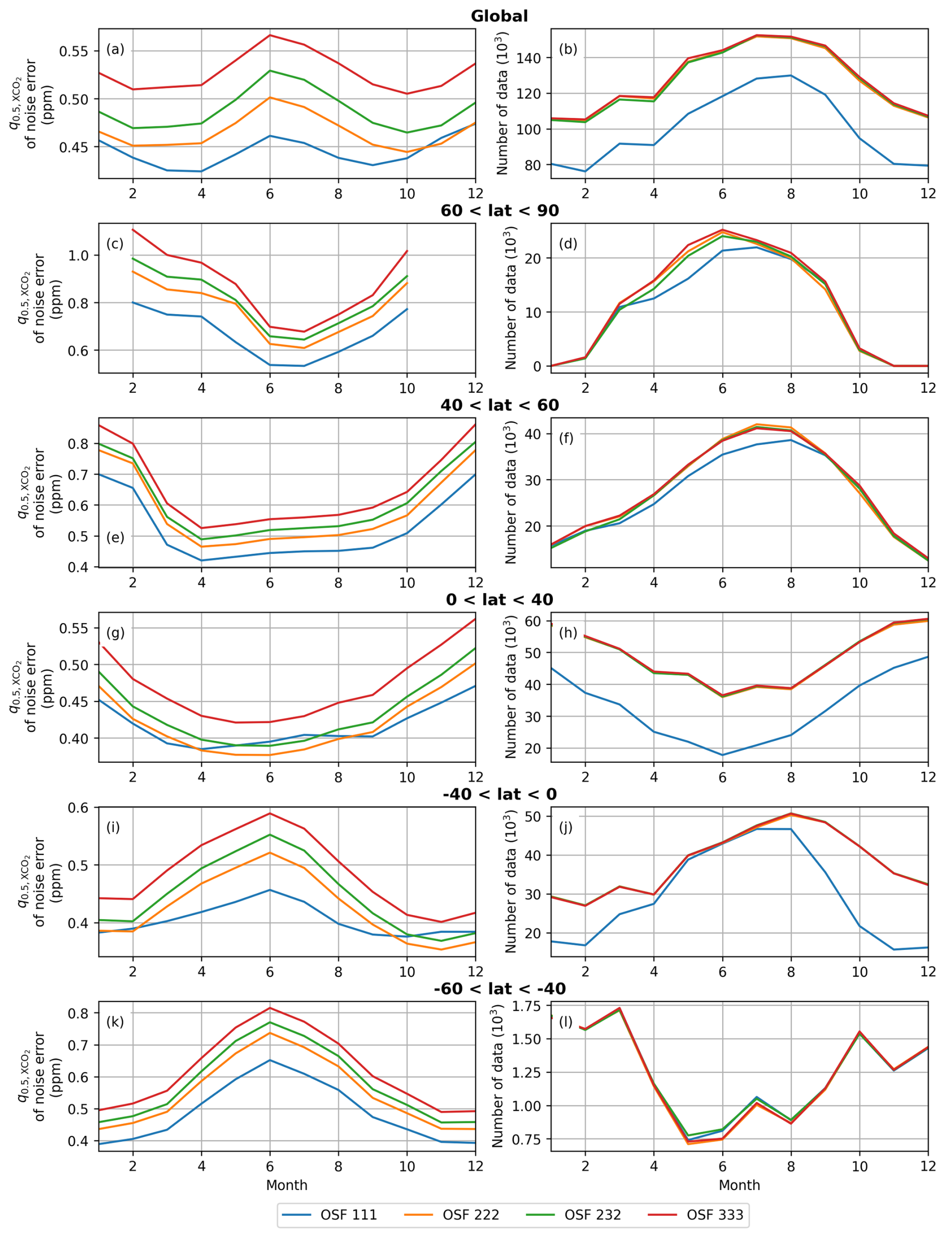
Figure 7 Time series of the monthly values for various latitude bands (rows) of the following for all OSF scenarios of Table 2: the panels in the left column show the monthly median (q_0.5) of the XCO₂ noise error. The panels in the right column illustrate the number of data that is left after filtering for saturation in the pre-processing step and after post-processing, i.e., data that have converged and are not filtered out during post-processing. In the latitude band between 60 and 90° S, data coverage is small; thus, it is not shown here.

We also analyzed the monthly evolution of the error and the number of spectral samples for all OSF scenarios after post-processing; see Fig. 7. Time series of the global monthly median XCO₂ noise error for all OSF scenarios can be found in panel a. The noise increases by a constant factor between scenarios OSF 222, 232 and 333. This is different for OSF 111 because the number of data (panel b) is decreased by about 20 % in this scenario due to the saturation filtering. The noise error shows a semi-annual cycle with maximum values in June and December, the respective summer months in each hemisphere. These peaks can be seen in the individual latitude bands shown in the rows of Fig. 7. In addition, most of the data loss in the OSF 111 scenario occurs in latitudes between 40° S and 40° N, where most deserts are located, consistent with previous findings. As the SNR is connected to the noise error (see Fig. 4) and the signal over deserts is usually larger than the average, the median noise error increases when the saturated spectra of desert regions are filtered out, which explains the anomalies in the noise error globally and in the near-tropical latitude bands (panels a, g and i). In all other latitudes, the median XCO₂ noise error increases with increased OSF in the SWIR bands, which are sensitive to changes in CO₂. The results of the northern mid-latitudes in Fig. 7e are the best approximation of the VEG50 scenario, which is based on typical mid-latitude vegetation conditions, like albedos and a solar zenith angle of 50°, and which defines the requirements for CO2M (ESA, 2020). Tests with VEG50 (not shown) showed XCO₂ noise values similar to those in the winter months of the panel: approx. 0.7 ppm for OSF 111, 0.77 ppm for OSF 222 and 0.88 ppm for OSF 333. Therefore, these results are consistent with the findings of this experiment.

As calculations of emissions depend linearly on the XCO₂ enhancement to some background value (e.g., Fuentes Andrade et al., 2024), the error in emission estimates scales linearly with the XCO₂ a posteriori noise of single soundings. Thus, the relative change in XCO₂ a posteriori noise is the same for uncertainties in the emissions. This was tested with a simple emission model in the scope of this study. As an example, using mid-latitude summer conditions where the median XCO₂ a posteriori noise error increases from 0.45 ppm (OSF 111) to 0.5 ppm (OSF 222), see panel e of Fig. 7 in June, it can be expected that the relative increase in the uncertainty of the emission due to noise is the same: 1.11 in the median, which can be larger for individual emission estimates.

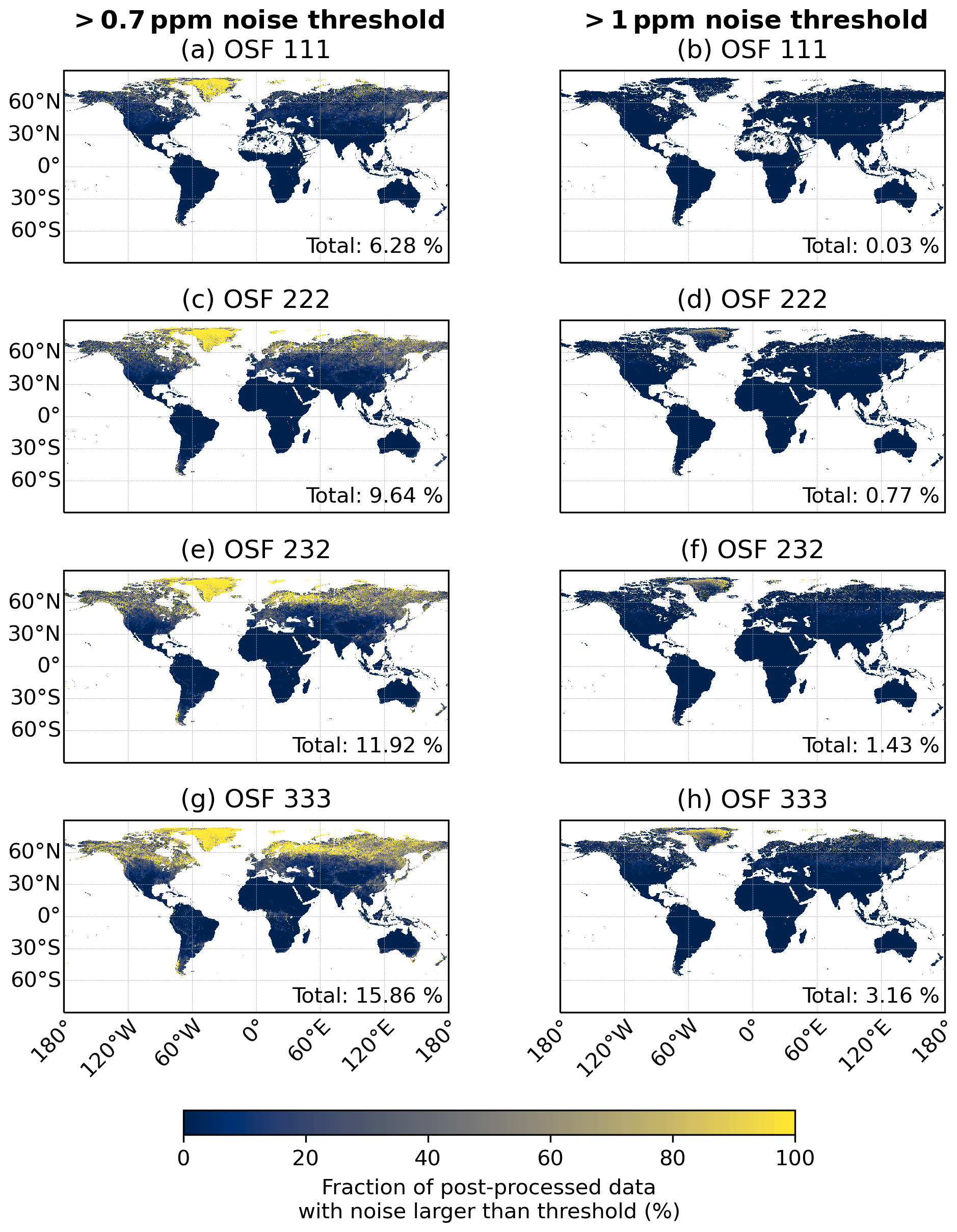
Figure 8 Fraction of spatial samples whose XCO₂ a posteriori noise error is larger than 0.7 ppm (left column), based on the precision requirement in ESA (2020), and 1 ppm (right column). The data are binned to a 0.4×0.4° latitude–longitude grid based on the CO2M spatial sample center coordinates. Note that the fraction is related to the data after post-processing in this figure. The global fraction is labeled “Total” in the panels.

For the estimation of emissions, high precision of the measurements is needed, which decreases with larger OSFs. Therefore, the columns of Fig. 8 show the fraction of post-processed data that is affected by a precision threshold of 0.7 and 1 ppm. This mostly affects the northern middle and high latitudes. Most of the post-processed data have an a posteriori noise error smaller than 1 ppm. The global fraction of affected spatial samples is smaller than 3.2 % for all OSF scenarios and is the largest in Greenland, where no significant sources of CO₂ exist. Furthermore, the possibility of the glint mode could change these results, especially over the snow-covered regions on Earth, because snow generally has an enhanced forward-scattering component (e.g., Mikkonen et al., 2024). On the other hand, 6 % of the post-processed data have a noise error larger than 0.7 ppm in OSF 111, about 9 % in OSF scenario 222, more than 11 % in OSF 232 and about 16 % in OSF 333. Hence, estimates of emissions over Scandinavia, Canada and northern Russia might be difficult when using an OSF larger than 2 because of the precision degradation there.

In summary, these results imply that increasing the OSF globally to values larger than 1 leads to minor decreases in the global median precision while increasing the coverage. Based on the simulated 1-year subset of radiance data used here, scenarios 111 and 222 seem to be favorable for CO2M in the future: although OSF 111 will lead to saturation over deserts and some snow-covered regions, the precision impact is the smallest among the scenarios, which might be of importance for the mid-latitudes. With OSF scenario 222, we found nearly global coverage with respect to saturation but a larger impact on the precision in the middle and high latitudes.

7 Summary and conclusions

The Copernicus Anthropogenic CO₂ Monitoring (CO2M) mission is a satellite constellation, with the first satellite expected to be launched in 2027. One of the operational greenhouse gas retrieval algorithms for CO2M will be the Fast atmOspheric traCe gAs retrievaL (FOCAL) algorithm. In this study, we analyzed the impact of scenarios avoiding saturation of the detector, which may occur, for instance, over bright scenes on the Earth's surface and which have to be filtered out during the retrieval so that the coverage is decreased. This can be avoided by increasing the number of read-outs per integration time step, i.e., increasing the oversampling factor (OSF), which, on the other hand, decreases the SNR of the measurement. We used idealized simulated radiances for this study, with the goal being to investigate the long-term impact of using different OSFs. This was done by examining saturation on a per-spatial-sample basis without considering any effect either from nearby bright scenes from the surrounding spatial samples or from nearby bright scenes outside the swath that could lead to saturation as well, such as stray light from nearby clouds. Clouds can lead to saturation as well, in which case the OSF might have to be increased for that scene.

We used a 1-year subset dataset of simulated radiances for conditions of 2015 to define scenarios of OSFs and then to investigate the impact on XCO₂ using FOCAL. Post-processing was adapted depending on the OSF used because changing the OSF changes the retrieval-related detector properties. Our assumption was to keep one OSF setting for the whole globe and year to avoid possible calibration difficulties due to changing OSFs during the operation and to keep the operation of the satellite as simple as possible.

We compared the maximum radiances with the OSF-specific maximum radiance that can be detected in all spectral bands in order to define scenarios of OSFs to be used in the long-term analysis. We found that saturation occurs in particular over deserts and parts covered by rocks. Scenarios increasing the OSF for all CO2M spatial samples to values between 2 and 3 in the near-infrared (NIR) and shortwave infrared (SWIR) bands were defined. These scenarios were referred to as OSFs 111 (baseline), 222, 232 and 333, corresponding to the OSFs set in the NIR, SWIR1 and SWIR2 bands, respectively.

We found that the decrease in signal-to-noise ratio (SNR) due to different OSFs has a wavelength-band-dependent impact on the XCO₂ a posteriori noise error, with the smallest sensitivity in the SWIR2 band. The impact on XCO₂ was analyzed with distributions of the global noise error estimates, which increased by a factor of 1.18 between OSF scenarios 111 and 333 and 1.06 between OSFs 111 and 222, which in the median is not large but leads to precision degradation in the northern high latitudes at the edge of emission estimation. The results showed that the filtered regions mostly include regions that are not known to have large emission sources. Therefore, the degradation of precision in these regions might be acceptable so that the assumption of a uniform OSF might also be relaxed and the OSF could be switched to OSF 222 over regions like deserts and to OSF 111 elsewhere.

This study used a fixed sampling period of 308 ms to meet the mission requirements. In principle, this value can be adjusted in order to get the optimum between SNR and saturation avoidance. Further investigations in the future could include a reduction in the sampling period instead of increasing the OSF. However, a smaller sampling period would further reduce the SNR, and synchronization of the CO2I/NO2I spectrometers might become more difficult with a smaller sampling period.

The results of this study are based on an idealized simulation of surface properties and the assumption of a perfect instrument. Thus, errors might be larger for real measurements, and the results shown here can only provide a first insight into the actual impact of changing the OSF when applied to real measurements. The analysis is limited to the nadir configuration over land, and further investigations for other foreseen geometries, like ocean glint, are needed in the future. In addition, the impact on emissions, especially in the northern high latitudes, such as Scandinavia, Russia and Canada, should be further investigated in more detail in the future. While the analysis of the saturation filtering is independent of the retrieval method used, further results will depend on the retrieval algorithm and are likely to be different for Fusional-P-UOL-FP and RemoTAP. As discussed, e.g., by Noël et al. (2024), the requirements concerning CH₄ are not as stringent as for CO₂, which is why we restricted the analysis to CO₂ in this study.

Overall, we found increases in coverage and decreases in precision when using OSFs larger than 1. Based on the idealized simulated radiances, the OSF 111 and 222 scenarios could be regarded as possible OSF scenarios for the CO2M mission for XCO₂, under the assumption of a fixed OSF setting independent of location. These results are intended to be used for the planning of the commissioning phase of CO2M.

Appendix A: Retrieval setup for the OSF scenarios

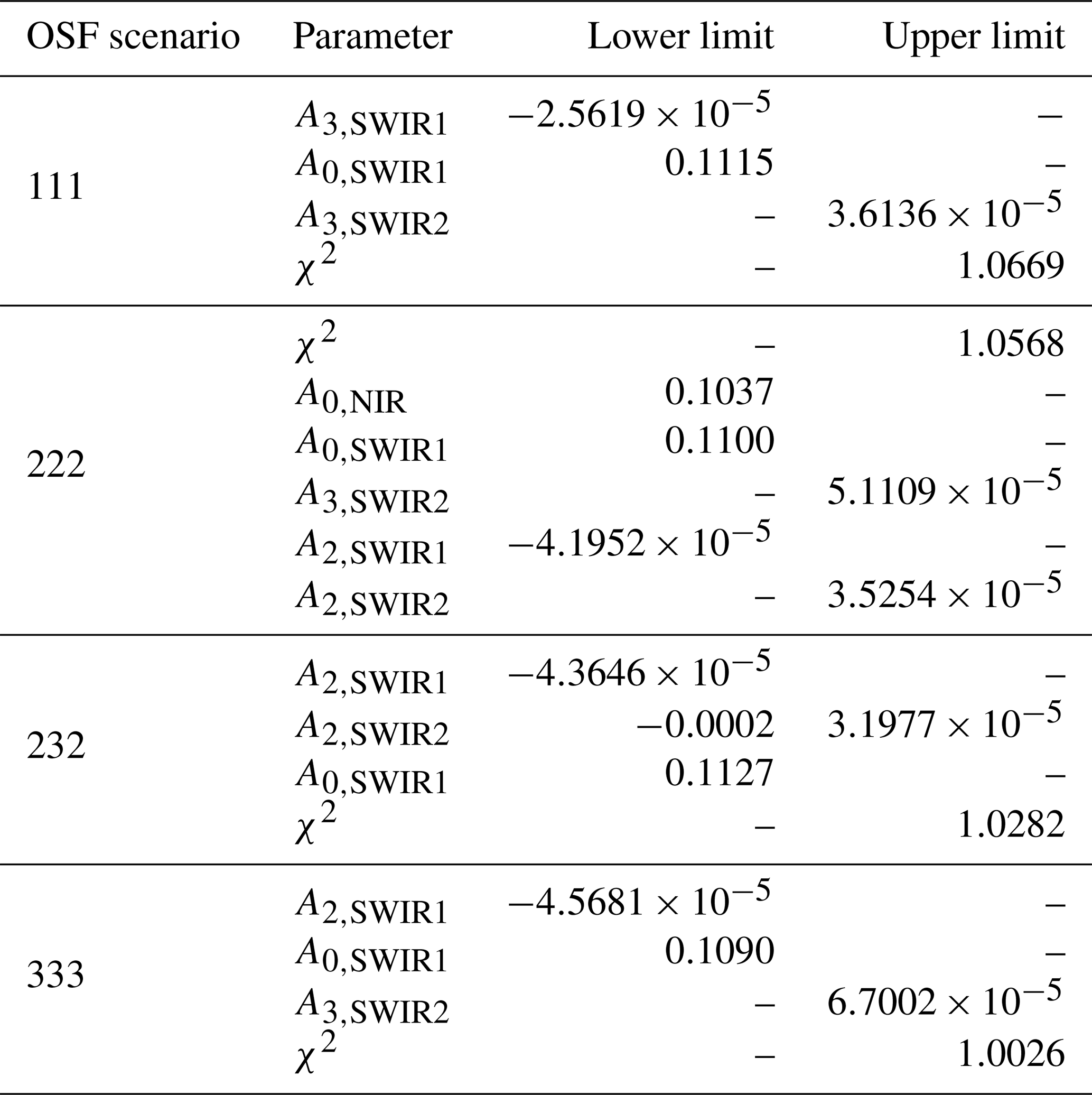
As discussed in Sect. 5, the retrieval setup depends on the OSF scenario. For the forward model error, we strictly followed the concepts outlined by Reuter et al. (2017a) and Noël et al. (2024). Table A1 summarizes the variables used and the corresponding limits of the variance filter applied during post-processing.

Table A1 OSF-dependent limits of retrieval variables applied during post-processing to minimize the overall variance, sorted by their relevance. The variables are albedo coefficients A_i,band of a second-order polynomial and the cost function χ². No limit is denoted with a dash. Note that the variable notation comes from Reuter et al. (2017a) and should not be confused with the parameter A of the SNR in the main text.

Appendix B: Impact of removing whole swaths instead of single spatial samples

The analysis in this study assumes that neighboring spatial samples in the swath are not affected when saturation occurs. As the stray-light correction is insufficient for the swath if saturation occurs in one spatial sample, there might be effects on neighboring spatial samples for CO2I/NO2I, which is why the analysis of saturation on the spatial coverage was re-calculated by excluding whole swaths instead of single spatial samples; see Fig. B1.

As can be seen, the total fraction of remaining data for OSF 111 is decreased significantly to about 47 % in comparison to Fig. 5, with a similar global distribution, and after post-processing, the remaining data are reduced to 34.5 % for OSF 111. This is expected because additional data are removed at a similar location where saturation was identified in Fig. 5.

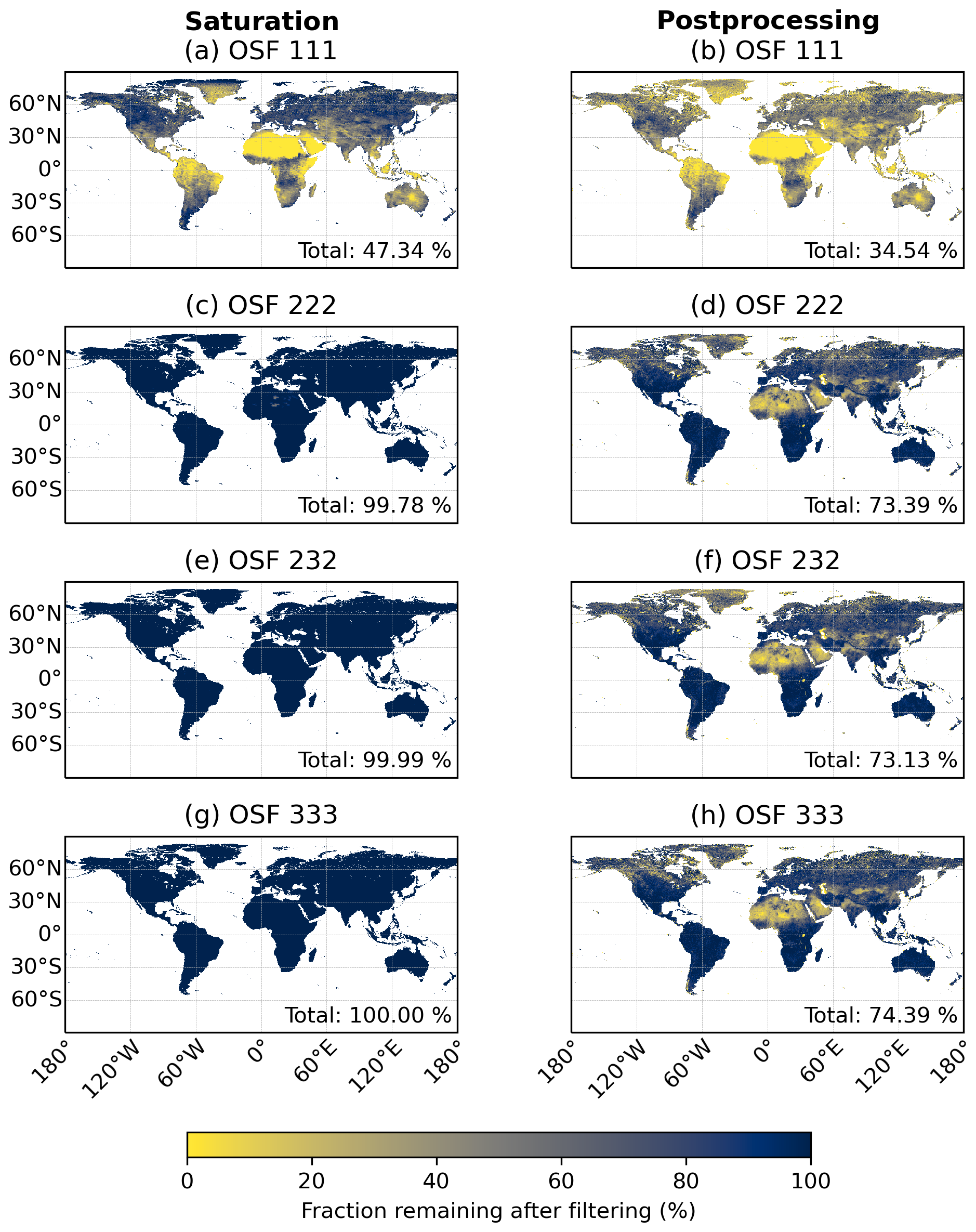
Figure B1 Same as Fig. 5 but removing whole swaths instead of single spatial samples.

Apart from the total number of measurements, the results showed only minor changes of the order of ±0.02 ppm in the XCO₂ precision.

Appendix C: Saturation and SNR for a range of sampling periods

As mentioned in Sect. 2, the selection of the sampling period t_samp is driven by CO2M mission requirements for spatial resolution and signal-to-noise ratios. In this appendix, we provide more details about these requirements, add saturation to the discussion, and generalize the analysis of saturation and SNR to different sampling periods.

The A and B values for calculation of the SNR are given for t_samp=308 ms and three OSFs. As parts of B depend on the integration time (see Eq. 6) and parts only depend on the OSF, these parts have to be extracted, which is done by a linear regression of B that depends on the OSF. Substituting $u=I_{\mathrm{dark}}+I_{\mathrm{Tb}}$ and $v=N_{\mathrm{RO}}^{\mathrm{2}}+N_{\mathrm{AD}}^{\mathrm{2}}+N_{\mathrm{VC}}^{\mathrm{2}}$ in Eq. (6) yields

$$\begin{array}{}\text{(C1)}& B=u\cdot \left[t_{\mathrm{samp},\mathrm{308}}-(\mathrm{OSF}\cdot t_{\mathrm{RO}})\right]+v\cdot \mathrm{OSF}.\end{array}$$

Here, the numbers in the indices indicate that the sampling period is constant (308 ms) in this equation, which is varied in the later part of this section. Rearranging for OSF as x-axis values yields

$$\begin{array}{}\text{(C2)}& B=(v-u\cdot t_{\mathrm{RO}})\cdot \mathrm{OSF}+u\cdot t_{\mathrm{samp},\mathrm{308}}.\end{array}$$

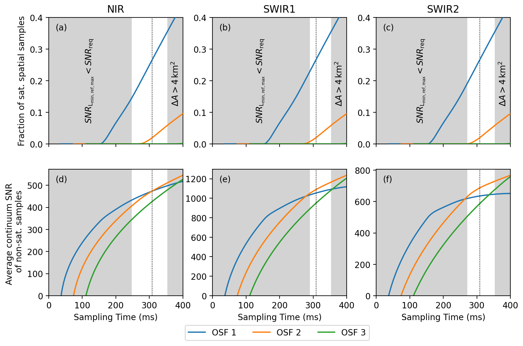
Figure C1 Saturation and SNR impact for a range of sampling periods. Gray-shaded regions: non-compliant with SNR and spatial footprint area requirements. (a, b, c) Fraction of saturated spatial samples in the global subset dataset for OSFs 1–3 in the (a) NIR, (b) SWIR1 and (c) SWIR2 bands. (d, e, f) Global average of the spectral maximum SNR of non-saturated spatial samples for OSFs 1–3 in the (d) NIR, (e) SWIR1 and (f) SWIR2 bands. The dashed vertical line depicts the sampling time of 308 ms that is used in the main text.

Linear regression with OSF on the x axis leads to a linear equation with slope m and intercept y₀, which can then be used to get the values for u:

$$\begin{array}{}\text{(C3)}& u={\displaystyle \frac{y_{\mathrm{0}}}{t_{\mathrm{samp},\mathrm{308}}}},\end{array}$$

and v:

$$\begin{array}{}\text{(C4)}& v=m+{\displaystyle \frac{t_{\mathrm{RO}}{y}_{\mathrm{0}}}{t_{\mathrm{samp},\mathrm{308}}}},\end{array}$$

for each detector pixel. With these equations, the B values can be calculated for all possible sampling periods. For A, the given values have to be divided by the integration time, cf. Eq. (5), where we use the values of OSF 1 and an integration time of 271 ms.

We first derive the sampling periods that are within the mission requirements of CO2M. The SNR requirement is given in ESA (2020) for specific radiance values L_min, L_ref and L_max in each wavelength band. We calculate the SNR using A and B for sampling periods between 0 and 400 ms and the radiance values from ESA (2020) using OSF 1. Note that we neglect the issue that changes in the sampling period will also change the size of the footprints. The sampling period where the SNR for all radiances is smaller than the required SNR, SNR_req, is the minimum value for the sampling period; see left gray-shaded region in the panels of Fig. C1. As shown in this figure, the sampling period has to be larger than about 295 ms to be compliant with the SNR requirements of CO2M in all wavelength bands.

On the other hand, the sampling period has an upper limit because of the requirement of a footprint area smaller than 4 km², as described in the main text. Using the ground speed of the satellite of 7 km s⁻¹ and the ACT footprint width of 1.8 km and considering that during the read-out time t_RO no signal is measured (cf. Fig. 1), we arrive at a sampling period of about 350 ms, which is the maximum to be used to be compliant with the spatial extent of a CO2M footprint (right gray-shaded region in the panels of Fig. C1).

Saturation (first row of Fig. C1) is evaluated for the complete 1-year subset dataset for all sampling periods and OSF scenarios. The fraction of spatial samples affected by saturation at at least one wavelength starts to increase from zero at t_samp≈150 ms for OSF 111 and increases with larger sampling periods. For OSF 222, the fraction starts to increase at around t_samp≈290 ms, with a slope that is smaller than that for OSF 111. No saturation can be found for OSF 333 in the shown range of sampling periods between 0 and 400 ms. The fractions at t_samp=308 ms (dashed black line) are consistent with the results from Table 1.

As a final step, we take all non-saturated spatial samples of the subset dataset and calculate their maximum SNR for all sampling periods, which corresponds to the SNR in the continuum range of the spectra in the respective wavelength band. The global average of all non-saturated spatial samples is shown in the second row of Fig. C1. Note that this analysis is different from Fig. 3, where only spatial samples were analyzed in which no saturation occurred in any OSF scenario. The SNR increases for larger sampling periods. The SNR can only be calculated if $\mathrm{OSF}\cdot t_{\mathrm{RO}}>t_{\mathrm{samp}}$; see Eq. (5). Since the SNR for saturated spectra cannot be calculated, but the spectra with saturation usually have the largest SNR, the average continuum SNR is decreased when filtering for saturation compared to non-filtered SNR. Hence, the global average SNR for OSF 1 becomes smaller than that for OSF 2 between about t_samp=290 and t_samp=310 ms, depending on the wavelength band, confirming the main result of this study that OSF 222 is a possible scenario for CO2M in the future.

In the requirement-compliant range of sampling periods (white background in the panels of Fig. C1), the increase in the SNR is small, and saturation should be avoided in general, so a sampling period as short as possible should be used. Therefore, a sampling period close to the minimum in the requirement-compliant region was chosen and is set to t_samp=308 ms.