the Creative Commons Attribution 4.0 License.
the Creative Commons Attribution 4.0 License.
 | 28 Jul 2025
Benchmarking and improving algorithms for attributing satellite-observed contrails to flights
Vincent Meijer
Rémi Chevallier
Allie Duncan
Kyle McConnaughay
Scott Geraedts
Kevin McCloskey
Condensation trail (contrail) cirrus clouds cause a substantial fraction of aviation's climate impact. One proposed method for the mitigation of this impact involves modifying flight paths to avoid particular regions of the atmosphere that are conducive to the formation of persistent contrails, which can transform into contrail cirrus. Determining the success of such avoidance maneuvers can be achieved by ascertaining which flight formed each nearby contrail observed in satellite imagery. The same process can be used to assess the skill of contrail forecast models. The problem of contrail-to-flight attribution is complicated by several factors, such as the time required for a contrail to become visible in satellite imagery, high air traffic densities, and errors in wind data. Recent work has introduced automated algorithms for solving the attribution problem, but it lacks an evaluation against ground-truth data. In this work, we present a method for producing synthetic contrail detections with predetermined contrail-to-flight attributions that can be used to evaluate – or “benchmark” – and improve such attribution algorithms. The resulting performance metrics can be employed to understand the implications of using these observational data in downstream tasks, such as forecast model evaluation and the analysis of contrail avoidance trials, although the metrics do not directly quantify real-world performance. We also introduce a novel, highly scalable contrail-to-flight attribution algorithm that leverages the characteristic compounding of error induced by simulating contrail advection using numerical weather models. The benchmark shows an improvement of approximately 25 % in precision versus previous contrail-to-flight attribution algorithms, without compromising recall.
- Article
(6914 KB) - Full-text XML
- BibTeX
- EndNote


Condensation trails (contrails) are the ice clouds that trail behind an aircraft as a result of the warm, moist engine exhaust mixing with colder, drier ambient air (Schumann, 1996). When the ambient air is sufficiently humid (i.e., supersaturated with respect to ice), these contrails can persist for several hours (Minnis et al., 1998). They perturb the Earth's energy budget by reflecting incoming solar radiation and reducing outgoing longwave radiation (Meerkötter et al., 1999). The net effect of all persistent contrails is estimated to be warming and of a magnitude comparable to the warming impact of aviation CO2 emissions (Lee et al., 2021).
Several mitigation options for the climate impact of contrail cirrus exist, such as the use of alternative fuels (Voigt et al., 2021; Märkl et al., 2024) and trajectory modifications (Mannstein et al., 2005; Teoh et al., 2020; Martin Frias et al., 2024). Although the latter approach, referred to as contrail avoidance, may lead to additional fuel burn and concomitant climate impacts, several simulation studies (Teoh et al., 2020; Martin Frias et al., 2024; Borella et al., 2024) have assessed this trade-off and conclude that this is a cost-effective mitigation strategy. These studies do, however, make use of forecast and reanalysis data to quantify the climate impact of contrails. While corrections to the weather data inaccuracies are applied sufficiently to draw the conclusions of the studies, other studies have demonstrated that these corrections are insufficient for the accurate prediction of formation and persistence of individual contrails by specific flights (Gierens et al., 2020; Geraedts et al., 2024; Meijer, 2024). Real-world avoidance trials have established the operational feasibility of avoiding detectable contrail formation using existing forecast models (Sausen et al., 2024; Sonabend et al., 2024), but they have also demonstrated that the forecasts are imperfect and that larger-scale trials will be necessary in order to determine whether the cost-effectiveness concluded by the modeling studies is achievable in practice.
Contrail avoidance trials are generally evaluated using contrail observations, such as those acquired by satellite imagers. The automated recognition of contrails is possible in infrared satellite images captured by both low-Earth-orbit and geostationary satellites (Mannstein et al., 1999; McCloskey et al., 2021; Meijer et al., 2022; Ng et al., 2024). Detections of contrails in geostationary satellite images are particularly interesting for the monitoring of contrail avoidance due to their high temporal resolution and broad spatial coverage, which allow one to track individual contrails over part of their lifetime (Vazquez-Navarro et al., 2010; Chevallier et al., 2023). However, imaging instruments aboard geostationary satellites such as GOES-16 (Goodman et al., 2020) have coarser image resolutions of approximately 2 km at nadir. This affects the number of contrails that are observable in these images (Driver et al., 2025) at any given time. Specifically, contrails are not observable at the moment they form; moreover, those that do eventually become observable require some time before they have become sufficiently large and/or optically thick. Previous studies using GOES-16 Advanced Baseline Imager (ABI) data indicate that the time taken to become observable is highly variable, generally ranging from 5 min to 1 h (Chevallier et al., 2023; Geraedts et al., 2024; Gryspeerdt et al., 2024). As a consequence, the contrail advects away from where it formed before becoming observable, which complicates the process of attributing it to the flight that formed it. The lack of altitude information associated with the observed contrails, owing to the satellite's 2D view of the 3D space, further enhances the difficulty of the problem. Once an observed contrail is attributed to an aircraft, this information can be used to study the relation between observed contrail properties and aircraft parameters (Gryspeerdt et al., 2024), evaluate the performance of contrail prediction models (Geraedts et al., 2024), train machine learning algorithms for better predictions of contrails (Sonabend et al., 2024), and monitor contrail avoidance trials.
Two recent contrail avoidance trials, Sausen et al. (2024) and Sonabend et al. (2024), each demonstrated a statistically significant reduction in the number of observed contrails when avoidance was performed. Neither of them, however, relied on automated attribution of contrails to flights when evaluating the trial: Sausen et al. (2024) evaluated the presence of detectable contrails in the satellite imagery for an entire airspace region, whereas Sonabend et al. (2024) relied on the time-consuming manual review of satellite imagery by the study's authors. Both studies emphasized the need for improved evaluation methods that are more scalable than what was used, in order to progress to the size and format of trial that could inform the operational requirements and impact of fleet- or airspace-wide contrail avoidance.
There has additionally been recent interest in establishing monitoring, reporting, and verification (MRV) systems for contrail climate impact, at the airspace, national, or continental levels. One example is the proposal for an MRV system for non-CO2 effects of aviation in the European Union (Council of European Union, 2024). Among the goals of these systems are to monitor the contrail impact of each airline and encourage its reduction. For any such implementation, there will be a need for both an assessment of the quality of contrail forecasts and accurate and scalable methods that can retrospectively determine contrail formation on a per-flight basis.
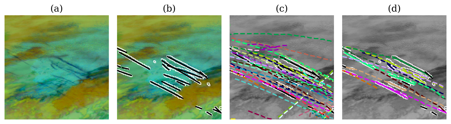
Figure 1A high-level visualization of a generic contrail-to-flight attribution process. All panes show a portion of a GOES-16 ABI image from 16:40 UTC (coordinated universal time) on 6 May 2019 over Ontario, Canada, rendered using the Ash color scheme to map infrared brightness temperatures to the visible spectrum. In panel (a), we see just the image, with some contrails visible in dark blue and some other clouds in yellow and brown partially obscuring some of the contrails. In panel (b), we show the result of running an automated contrail detector on the image, with the detected contrail pixels outlined in white and the results of linearizing the detector outputs as black line segments. Notably, some contrails appear segmented due to occlusion from other clouds. In panel (c), we take all flight paths that passed nearby in the preceding 2 h and simulate their advection to the capture time of the GOES image. This estimates the expected location of a hypothetical contrail that each flight formed. Each advected flight is shown using a unique color, while the contrails are still in black with white outlines (we render the satellite image in grayscale to improve visibility). Note that there is not a perfect alignment between observed contrails and flights; in some cases, there appear to be many candidate matches, whereas there appear to be none in other cases. In panel (d), we show the results of a contrail-to-flight attribution. Contrails that have been attributed are now color-coded to match the flight to which they were attributed, and only those flights are shown. Contrails in black were not attributed to a flight. The attributed flights are not always what appeared to be the best match in panel (c), as the attribution algorithm can take additional signals, like temporal dynamics, into account.
Several approaches have been developed to address the problem of automatically attributing contrails observed in satellite imagery to flights. All of them to some degree follow the approach visualized in Fig. 1: contrails visible in geostationary imagery (Fig. 1a) are detected and often then individually transformed into representative line segments (Fig. 1b); joined with flight tracks advected with weather model data (Fig. 1c); and, finally, attributed to flights using some form of optimization algorithm (Fig. 1d). Duda et al. (2004) apply this approach using the minimum average perpendicular distance between the advected flight track and the observed contrail in a single satellite frame for determining attribution. Geraedts et al. (2024) build on this approach by adding rotational and age-based components to the optimization. Gryspeerdt et al. (2024) first track contrail detections across frames using wind data at a fixed altitude, and they then use the resulting chains of detections to identify flights that passed through before the earliest detection and whose advected tracks are within distance and angle thresholds of the set of detections. Chevallier et al. (2023) replace the linearizations with contrail instance masks and then perform a discrete optimization that simultaneously tracks the contrail masks over successive satellite images and attributes them to the flight that formed them. We observe that, in all of these approaches, the advected flight that is closest to a given contrail detection, in some cases subject to additional temporal constraints, is presumed to have formed the contrail. In this study, we will show that the error in the simulated advection of the flight increases as the contrail ages, implying that the advected flight nearest to the contrail detection is often not the correct attribution.
We further observe that these previous studies carried out limited to no evaluation of the performance of these algorithms. Of the four studies mentioned, only Geraedts et al. (2024) provide any quantitative evaluation, using 1000 manual labels that indicated whether a flight segment formed a contrail or not. Ideally, such labels should also provide information on which flight segment formed which particular observed contrail. Benchmarking these attribution algorithms is complicated by the lack of ground-truth data. As discussed, the moment of formation of a particular contrail is not observed in geostationary satellite imagery. A ground-truth dataset for these attribution algorithms therefore requires observing the moment of formation using some higher-resolution instrument, possibly a ground-based camera, and following the contrail until it becomes observable in the satellite imagery of interest. While ground-based contrail observation datasets exist (Gourgue et al., 2025; Low et al., 2025; Schumann et al., 2013), including a small one that matches its observations to those of a geostationary satellite (Mannstein et al., 2010), no dataset of sufficient size and diversity to suit our needs is available at the time of writing. Even with such a dataset in hand, the metrics used to evaluate the performance of a contrail-to-flight attribution algorithm and their implications for downstream usage of the algorithm output data are relatively underexplored. For example, an attribution algorithm that is conservative with respect to the number of contrail-to-flight attributions that it assigns by prioritizing quality over quantity may be suitable for comparing the per-flight predictions of a contrail forecast model to satellite observations. However, such an algorithm would perhaps be less suitable for the evaluation of a large-scale contrail avoidance experiment using satellite imagery. Additionally, one attribution algorithm may outperform others only under certain circumstances (such as high air traffic density), which could further motivate choosing a particular approach over others.
We thus conclude that there are several relevant applications for attributing satellite-observed contrails to the flights that formed them, but this potential has not yet been fully realized, in part due to the combination of the inability to assess the performance of automated approaches and the limited scalability of the manual counterparts. This study, therefore, introduces a large-scale benchmark dataset of synthetic contrail detections with predetermined flight attributions, named “SynthOpenContrails”, and a new, scalable attribution algorithm, named “CoAtSaC” (short for “Contrail Attribution Sample Consensus”). In Sect. 2, we introduce SynthOpenContrails, how it is generated, and how to apply it to benchmarking attribution performance. In Sect. 3, we describe CoAtSaC and show how to use SynthOpenContrails to tune its performance. Section 4 shows that CoAtSaC provides substantial improvement when compared to existing approaches when evaluated on the new benchmark. It further shows how the size and diversity of SynthOpenContrails enables one to verify the scalability of a particular attribution algorithm and to study its performance under differing conditions, such as different contrail densities, contrail altitudes, seasons, and times of the day.
We start by addressing the question of how to determine the skill level of a given attribution algorithm. Ideally, we would use a dataset of ground-truth contrail attributions in geostationary imagery to tune and evaluate our attribution algorithm. Currently, no such dataset exists, as it is an extremely challenging task even for a skilled human to perform without additional evidence. In the absence of such a dataset, we propose a synthetic contrail dataset. Specifically, we aim to provide a set of synthetic contrail detections that can be directly input to an attribution algorithm. The synthetic contrail detections should be as statistically similar as possible to real detections, while specifying which flight created each contrail. While not a strict requirement, we choose to produce a dataset corresponding to the capture times and pixel grid of real satellite scans, as that allows for both quantitative and qualitative comparison with the real contrail detections from the corresponding scan.
Importantly, these synthetic contrail detections are simulating a particular detection algorithm run over imagery from a particular geostationary satellite, including the flaws of both. They are not attempting to model a physical reality or what an expert human labeler might produce for a given satellite image. It is not a goal of this dataset to have exactly the same flights that formed detectable contrails in reality also form contrails in this dataset, nor do the synthetic contrails need to end up being in exactly the same locations as the contrails that the detection algorithm finds in the same scene. Ultimately the critical element is that the dataset has statistics as similar as possible to the real detections, in terms of contrail density, dynamics, detectable lifetime, and advection error relative to the weather model data, so that we can measure the attribution algorithm's performance across all scenarios that it is likely to encounter with real contrail detections. An added benefit that the dataset provides is access to the physical properties of the synthetic contrails that allow one to study the attribution algorithm's performance as a function of these properties.
While the resulting dataset takes the form of contrail labels corresponding to satellite imagery, due to the aforementioned caveats, it is not suitable for training contrail detection models and is, thus, intended only for use in contrail attribution algorithms, where the labels need not align with actual satellite radiances.
The dataset described here, which we name “SynthOpenContrails”, is tuned towards the performance of the contrail detection algorithm introduced along with the OpenContrails dataset in Ng et al. (2024), specifically when applied to the GOES-16 ABI Full Disk imagery (Goodman et al., 2020). The Full Disk imagery covers much of the Western Hemisphere, with approximately 2 km nadir spatial resolution and scans every 10 min. The Ng et al. (2024) algorithm uses a convolutional neural network to produce a prediction that each satellite pixel contains a contrail and thresholds the results to produce a binary mask. It then fits line segments to the individual contrails in the mask.
The approach presented here for generating the synthetic contrail detections should be adaptable to other detection algorithms and other satellites, but some details and parameter values may need to change. We also expect that attribution algorithms built around other detection methods should still be able to use SynthOpenContrails in its present form, and we demonstrate this in Sect. 4 by evaluating the Chevallier et al. (2023) algorithm with only minor modifications.
2.1 Data
The data used to produce the synthetic contrails consist of flight paths and historical weather data. We generate the dataset for the spatial region used in Geraedts et al. (2024), which covers roughly the contiguous United States, bounded by great-circle arcs joining 50.0783° N, 134.0295° W; 14.8865° N, 121.2314° W; 10.4495° N, 63.1501° W; and 44.0734° N, 46.0663° W. The dataset is designed to enable attribution algorithms to run over time spans that are sampled throughout the year between 4 April 2019 and 4 April 2020, divided into 84 time spans of between 4 and 22 h long, aiming to capture seasonal, day-of-week, and diurnal effects on contrail formation, requiring a minimum of 36 h of separation between time spans to ensure no overlap of flights or contrails between time spans. These time spans, specified in Appendix F, are almost identical to those used in Geraedts et al. (2024), but a few have been changed slightly to avoid GOES-16 ABI outages. To accommodate attribution algorithms that rely on temporal context, we also generate synthetic contrails for 2 h before the start and 3 h after the end of each time span, but we exclude these buffer periods from the benchmark metrics.
2.1.1 Flight trajectories
We use flight trajectories provided by FlightAware (https://flightaware.com, last access: 17 July 2025). This includes a mixture of Automatic Dependent Surveillance–Broadcast (ADS-B) data received by ground-based stations and Aireon satellites (Garcia et al., 2015). For the purposes of benchmarking contrail attribution, it is critical to recognize that these data are incomplete, as they may lack information on particular flights because operators may request their data to be obfuscated or excluded. The implication is that there may be detectable contrails formed by flights that are missing from the data, and the benchmark needs to assess whether the attribution algorithm can handle these contrails appropriately and avoid incorrectly attributing them to the best-matching flight that is in the data. We assume that it is unknown what fraction of flights are missing or whether they are in some way biased with respect to likelihood of persistent contrail formation. Our tuning and benchmarking protocols described in Sects. 2.3 and 3.5 take this into account.
In order to provide spatiotemporal context that an attribution algorithm might need in order to resolve the attributions for contrails at the borders of the space–time regions provided by the dataset, we consider all flight waypoints that were flown at any point between 6 h before the start of each time span and 3 h after it ends. We also dilate the spatial region by 720 km in each direction, to allow contrails formed by flights outside the region to advect in from all directions without presuming anything about the wind direction. We resample each flight to CTflight=5 s in between waypoints, such that there will end up being roughly two waypoints per GOES-16 ABI pixel at typical aircraft speeds.
2.1.2 Weather data
In selecting weather data that will be used to determine synthetic contrail formation, dynamics, and evolution from the candidate flights, it is important that we do not use the same weather data as are used for flight advection in the attribution algorithm itself, as that would result in having an unrealistically low advection error. As the majority of recent approaches use the nominal ERA5 reanalysis product (Hersbach et al., 2020) from the European Centre for Medium-Range Weather Forecasts (ECMWF) for attribution, we use the control run of the ERA5 Ensemble of Data Assimilations (EDA), which has a coarser resolution than the nominal ERA5 reanalysis product. The ensemble data are at 3 h intervals and a 0.5° spatial resolution, and they are vertically discretized to 37 pressure levels that are separated by roughly 25–50 hPa. We unintentionally excluded the levels between 450 and 975 hPa, which led to some minor weather interpolation artifacts at the low end of the contrail formation altitudes (see Sect. 4.2).
The EDA control run does share an underlying model with the nominal ERA5 reanalysis; as such, shared systematic biases may exist that would not exist when relating the nominal ERA5 reanalysis to real contrail observations. See Appendix B1 for a further discussion of the appropriateness of selecting this source of weather data. Future research is necessary to identify or generate a source of weather data that achieves all of the necessary error characteristics in a fully unbiased fashion.
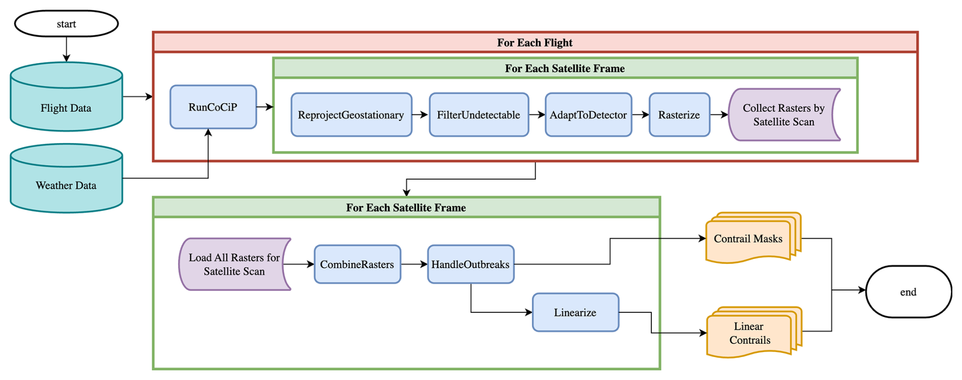
Figure 2A flow diagram of the process for generating synthetic contrails. The initial stages operate independently over each flight and determine the contributions of each flight to each relevant satellite scan. The later stages combine information from all flights that contribute to a given satellite scan and produce a contrail mask and a set of linear contrails for that scan.
2.2 Dataset generation
The process for generating the synthetic contrail detections is visualized in Fig. 2. We summarize each subroutine in the following, with further details found in Appendix A:
-
RunCoCiP. We simulate contrail formation and evolution using CoCiP (Schumann, 2012), which is a Lagrangian model simulating contrail formation and evolution, as implemented in the pycontrails library (Shapiro et al., 2024). We configure pycontrails as specified in Appendix A1. We need CoCiP to provide outputs for each flight at the times when the GOES-16 ABI Full Disk scan would have captured it. We note that the GOES-16 ABI does not capture the Full Disk scan instantaneously at the nominal scan time; rather, it captures it as 22 west-to-east swaths, starting in the north and moving south over the course of 10 min (see Appendix B2). This approach can be generalized to other geostationary satellites, as they have similar scan patterns (Okuyama et al., 2015). Each pixel then has a “scan-time offset”, based on when its location would be captured by the GOES-16 ABI relative to the nominal scan start time (Meijer et al., 2024). We do not know which pixels will capture a contrail formed by a given flight before running CoCiP. Furthermore, pycontrails can produce outputs only at fixed time intervals. Thus, in order to capture the outputs we need at the times corresponding to GOES-16 scans with the correct scan-time offsets, we configure pycontrails to produce outputs at 30 s intervals for the duration of the longest-lived contrail formed by the provided flight. If a flight does not form a contrail according to CoCiP, pycontrails will have no outputs, so we do not consider this flight any further. For flights that do form contrails, pycontrails outputs contrail properties for each contrail-forming input flight waypoint at each 30 s time step. We are, however, only interested in the properties that would manifest at the times that the GOES-16 ABI would capture the contrail. Therefore, we compute the scan-time offset corresponding to the location of each output and then select just the time step that is closest to each satellite scan plus scan-time offset for each waypoint. This results in a maximum of 15 s of error, which is negligible for our purposes (see Appendix B3). At this stage, we split up each flight's outputs according to the corresponding satellite scan and subsequent subroutines operate on them each independently.
-
ReprojectGeostationary. The goal of this subroutine is to reproject CoCiP's outputs from its native frame of reference to the perspective of the geostationary imager. CoCiP computes the parameters of the contrail plume cross-section at each flight waypoint such that attributes like width and optical thickness are measured along a viewing ray that passes directly through the center of the contrail to the center of the Earth. In order to render off-nadir contrails in the perspective of a geostationary satellite, we need to recompute these values using the viewing ray of the instrument. The details of how this is accomplished are given in Appendix A2.
-
FilterUndetectable. This subroutine's purpose is filtering CoCiP's outputs to just those that the Ng et al. (2024) detector would be likely to find if a contrail with these physical parameters were captured by the GOES-16 ABI. This amounts to codifying whether the training data for the detector would have included a label for this contrail. It computes a per-waypoint detectability mask, considering a few criteria, as detailed in Appendix A3.
-
AdaptToDetector. Before actually rasterizing the CoCiP data, we apply some adaptations directly to CoCiP's outputs, in order to better reflect the behavior of the detector being emulated. These are specified in Appendix A4.
-
Rasterize. In this subroutine, we map the filtered and adapted CoCiP outputs to pixel values in the geostationary imager's native projection and resolution. The most important component is determining what quantity should be rasterized in order to best imitate the detector. As the Ng et al. (2024) detector exclusively operates on longwave infrared bands, when estimating detectability, we need not account for factors affecting shortwave bands such as solar insolation; the quantity that we can extract from CoCiP that will best reflect detectability is, therefore, opacity. According to the Beer–Lambert law (Beer, 1852), opacity can be expressed as , where τ is the contrail optical depth produced by CoCiP. Appendix B5 discusses the appropriateness of applying the Beer–Lambert law here. The actual rasterization process adapts the process described in Appendix A12 of Schumann (2012) to geostationary satellite imagery. This is detailed in Appendix A5. The output of this subroutine is an opacity value κras for each pixel in the geostationary image that a flight contributed to in a single frame, along with the relevant CoCiP metadata for each waypoint that contributed to the pixel.
-
CombineRasters. We can then combine the rasters for all flights at the same time step, keeping track of the per-flight contrail parameters contributing to each pixel for later analysis. For simplicity, we resolve different flights contributing to the same pixel in the final raster by taking the maximum. The more correct approach would be to sum the optical thicknesses before converting to opacity, but CoCiP does not model these inter-flight effects and, in practice, it does not matter much for our use case. In order to simulate some of the smoothing effect that the detector has over the relatively noisy satellite imagery, we apply a spatial Gaussian blur, with a standard deviation of 1 pixel, without allowing any zero-valued pixels to become nonzero. We produce a binary contrail mask by thresholding the raster by .
-
HandleOutbreaks. This subroutine addresses the mismatch between how CoCiP and the Ng et al. (2024) detector operate in regions of very high contrail density, which we refer to as “contrail outbreaks”. Generally CoCiP will cover the entire region in contrails, to the point where individual contrails cannot be identified, while the detector will only identify the few most optically thick contrails. Appendix A6 details how we adapt these regions to behave more like the detector.
-
Linearize. In this subroutine, we map the rasterized opacities, which include per-pixel attribution metadata, to linear contrail segments that can be used in a contrail-to-flight attribution algorithm. This process is a close analog to the processing that Ng et al. (2024) applied to real satellite imagery and the resulting detector outputs, although with some additional bookkeeping. The full process is described in Appendix A7.
The final dataset consists of a set of synthetic linear contrail detections, each labeled with the flight that formed it, as well as other potentially useful physical properties derived from CoCiP. The full rasterized contrail mask is also available for each satellite frame, although we only use the linearized outputs in this study.
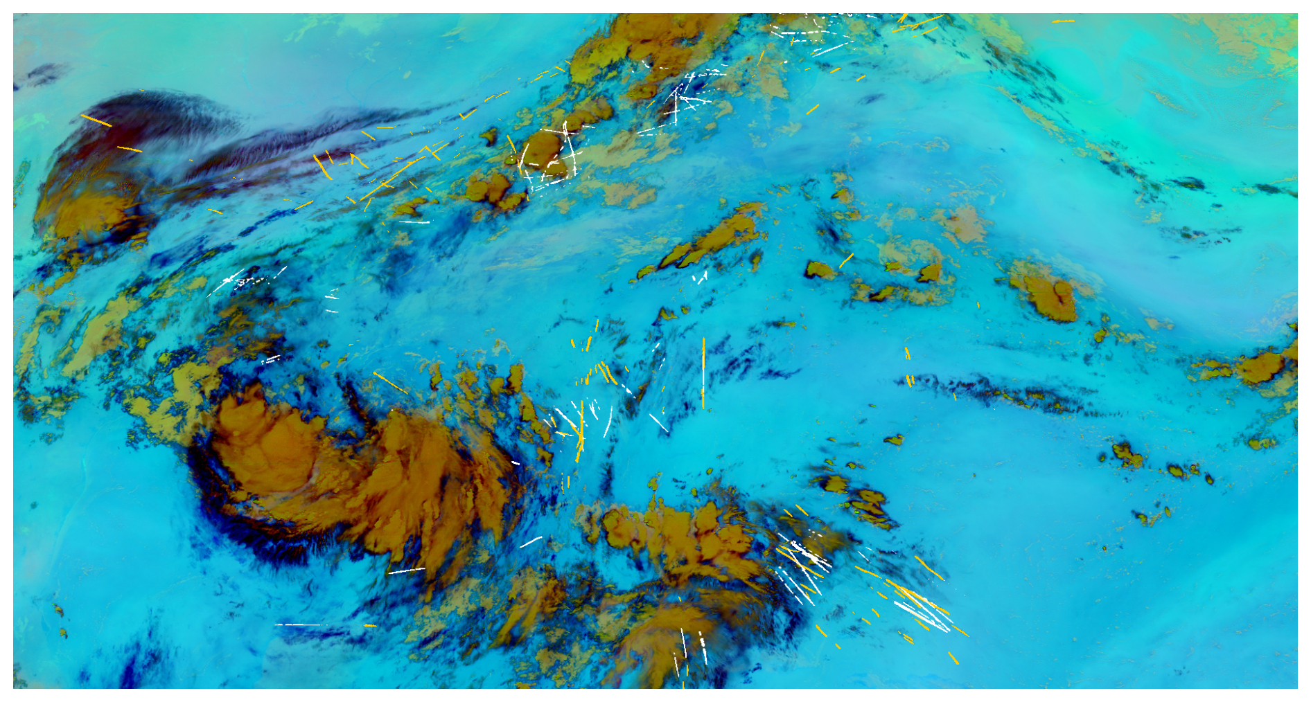
Figure 3An Ash-color-scheme false-color GOES-16 ABI image taken at 12:40 UTC on 11 July 2019 over the southeastern United States, showing the contrail mask produced by the Ng et al. (2024) detector (yellow) and the SynthOpenContrails mask (white). While the SynthOpenContrails contrails generally appear in the same regions as the detected contrails, there is far from perfect alignment, but that is unnecessary for the purposes of this dataset.
2.3 Tuning the synthetic dataset parameters
The pipeline that we have described for generating synthetic contrails includes a number of parameters whose values need to be determined. The intention here is to allow the same fundamental approach to be used to produce synthetic contrails that emulate different detection algorithms or different satellite imagers, just by setting different values for the parameters. As mentioned previously, for SynthOpenContrails, we produce synthetic contrails using the actual flights and weather model outputs corresponding to the capture times of real GOES-16 ABI Full Disk images. This allows us to tune towards matching the behavior of the Ng et al. (2024) detector on the real data.
Importantly, we divide the 84 time spans for which the dataset is generated into train, validation, and test splits, with 28 time spans each, as specified in Appendix F. This allows us to tune the dataset itself on one split, while using another split to verify that we have not “overfit” to the scenes in the split used for tuning. When the dataset is later used for tuning and benchmarking attribution algorithms, the same splits will again be useful to avoid overfitting.
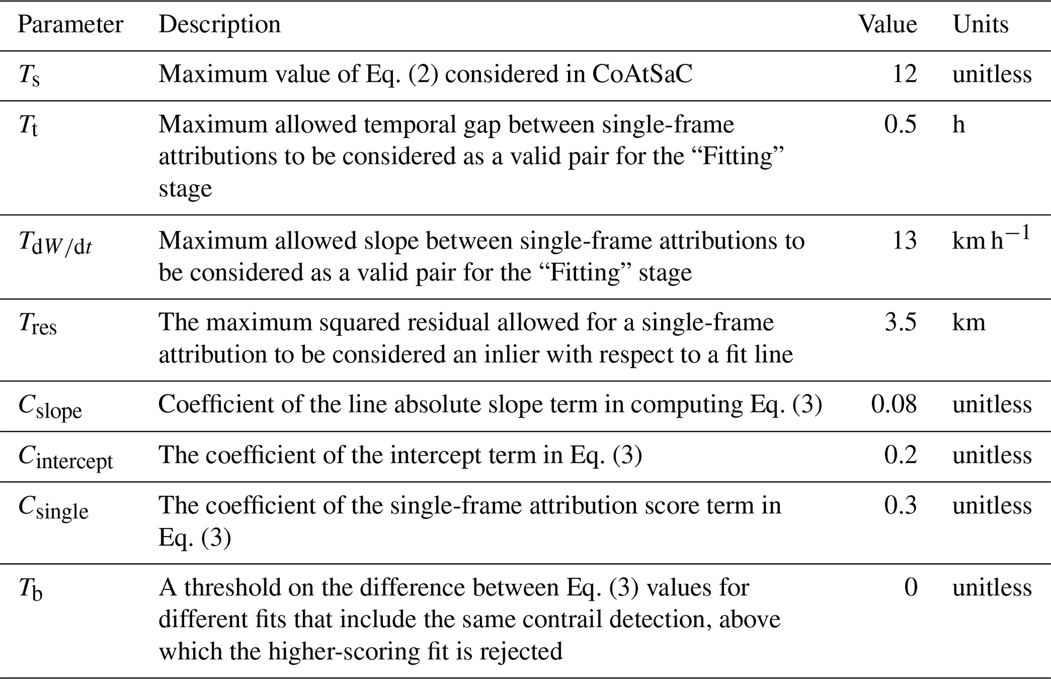
We manually tune to quantitatively match the statistics for number of contrail pixels and number of linear contrails per frame. We can further qualitatively compare by overlaying the real and synthetic contrail masks on sequences of GOES-16 ABI imagery. We use the Ash color scheme, as used previously in Kulik (2019), Meijer et al. (2022), and Ng et al. (2024), to map infrared radiances to RGB imagery that makes optically thin ice clouds, like contrails, appear in dark blue. An example frame of this imagery with both real and synthetic detections overlaid is shown in Fig. 3. For tuning purposes, we compute the real and synthetic contrail detections for the full validation set of time spans and apply our comparisons over those. We note that there are likely multiple sets of parameters that match our real data equally well, and the parameters used for SynthOpenContrails are just a single instantiation of this. For example, there is likely a set of parameters that allow contrails to be detectable at an older age by increasing the width or age thresholds inside FilterUndetectable and AdaptToDetector but that compensate for the resulting increase in contrail density by having higher thresholds for rasterized contrail opacity. Therefore, we caution against attempting to extract physical insights from SynthOpenContrails, as it has been designed only for evaluating contrail-to-flight attribution and is, in essence, a filtering of CoCiP simulations. The tuned parameter values that we use for generating SynthOpenContrails are in Table 1.
Table 1The parameter values used for generating SynthOpenContrails. Note that many of the parameters are introduced in Appendix A.
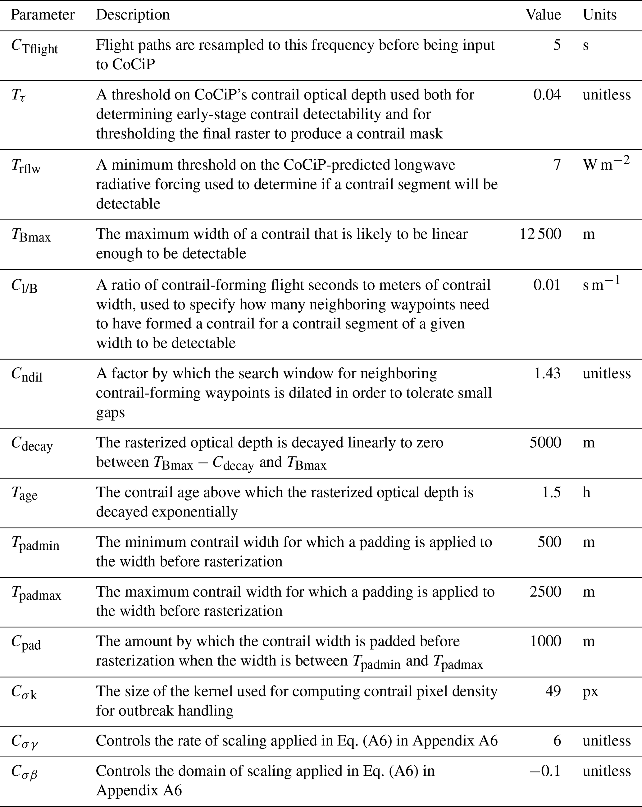
Table 2Statistics of the SynthOpenContrails splits. Values for the corresponding detector outputs on real satellite imagery are in parentheses, where applicable.
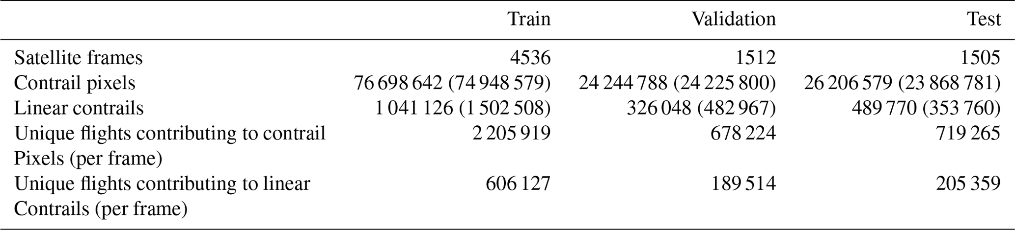
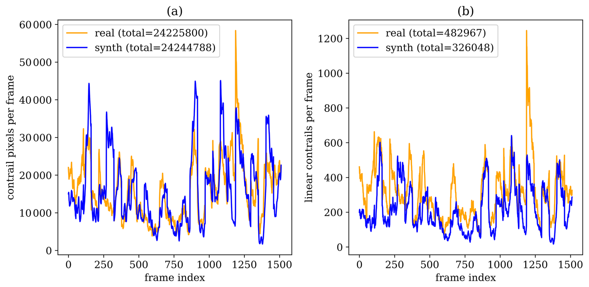
Figure 4Comparisons of contrail statistics between the outputs of the Ng et al. (2024) detector run on GOES-16 ABI imagery (in orange) and SynthOpenContrails (in blue), shown for satellite frames in the validation split. Panel (a) presents the number of contrail pixels per frame. Panel (b) shows the number of linear contrails per frame.
2.4 Properties of the SynthOpenContrails dataset
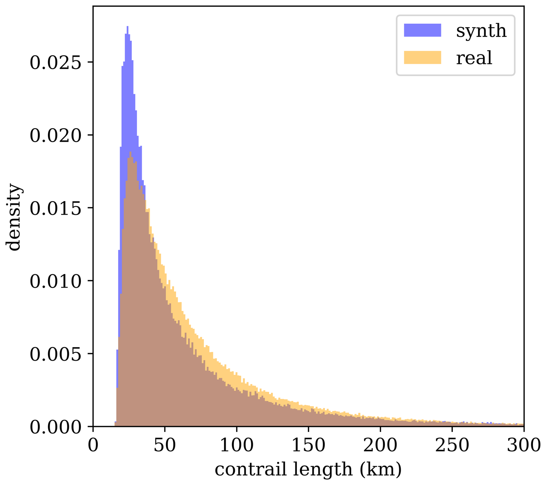
We show some top-level statistics comparing SynthOpenContrails to real detections for the same space–time regions, per dataset split in Table 2. We can also look at the per-frame contrail pixel and linear contrail counts, which are shown for the validation set in Fig. 4. The pixel counts in aggregate are very similar: there are only a few time spans during which SynthOpenContrails has meaningfully more contrail pixels and one notable span during which the real detection masks have many more pixels. On the whole, the peaks and valleys align very well. The linear contrail counts also match the overall trends, but the total counts are somewhat farther apart. The vast majority of the discrepancy comes from a single time span with a large outbreak, during which our adjustments to reduce the number of synthetic contrails in outbreaks seems to have overcompensated. We hope that future work can find a better approach to handling these cases. We can also compare the lengths of the linear contrails between real data and SynthOpenContrails, as shown in Fig. 5. The distributions match quite well, but SynthOpenContrails skews slightly shorter.
We also qualitatively evaluated the dataset with respect to how well it matches the Ng et al. (2024) detector outputs for the corresponding GOES-16 ABI scans, using visualizations like Fig. 3. We compared the geographic distribution of contrails, temporal dynamics, and the appearance of individual contrails in the mask. Of these characteristics, all appeared qualitatively similar, in the authors' opinion, with the exception of certain aspects of individual contrail appearance, as expanded upon below. We observe that the SynthOpenContrails contrail detections generally appear in the same regions as the real detections, but there is far-from-perfect alignment. While there are a few instances in which the SynthOpenContrails mask actually exposes contrails visible in the Ash-color-scheme imagery that the detector missed, the vast majority of the time the real detector better reflects what a skilled human would see in the satellite imagery. This is consistent with previous work (Gierens et al., 2020; Agarwal et al., 2022; Geraedts et al., 2024) which found that weather model data have difficulty predicting contrail formation at the per-flight level. The temporal dynamics from frame to frame do appear qualitatively similar to those of real detections. We reiterate that, for the purposes of our contrail-to-flight attribution system benchmark, it is not necessary that SynthOpenContrails be correct with respect to which flights actually formed contrails; it is only necessary that the distribution of properties of the synthetic data are similar to the real data. The individual synthetic contrails look qualitatively fairly similar to their detector-produced counterparts in overall form. The most noticeable difference is that the synthetic contrails have a slightly higher rate of appearing discontinuous. This likely arises from CoCiP evaluating each waypoint pair independently, in contrast with the smoothing tendencies of the detector. This could perhaps be rectified by a slight blurring of the CoCiP outputs across neighboring waypoints prior to rasterization. The fact that more discontinuous contrails are present in SynthOpenContrails masks does not affect CoAtSaC, as it only utilizes the linearizations of the contrail mask, which are for the most part unaffected by the discontinuities. Any attribution algorithm that directly uses the pixels within the contrail mask, however, may be affected, and this discrepancy should therefore be explored in greater detail for such approaches.
2.5 Benchmark metrics
Here, we define a set of metrics employed as the top-line results when SynthOpenContrails is used to benchmark attribution algorithm performance. The metrics are divided into per-contrail metrics and per-flight metrics. Generally the per-flight metrics will better assess the binary determination of whether a flight formed a contrail, while the per-contrail metrics will be more suitable for accounting for the number of contrails formed and how long they persisted.
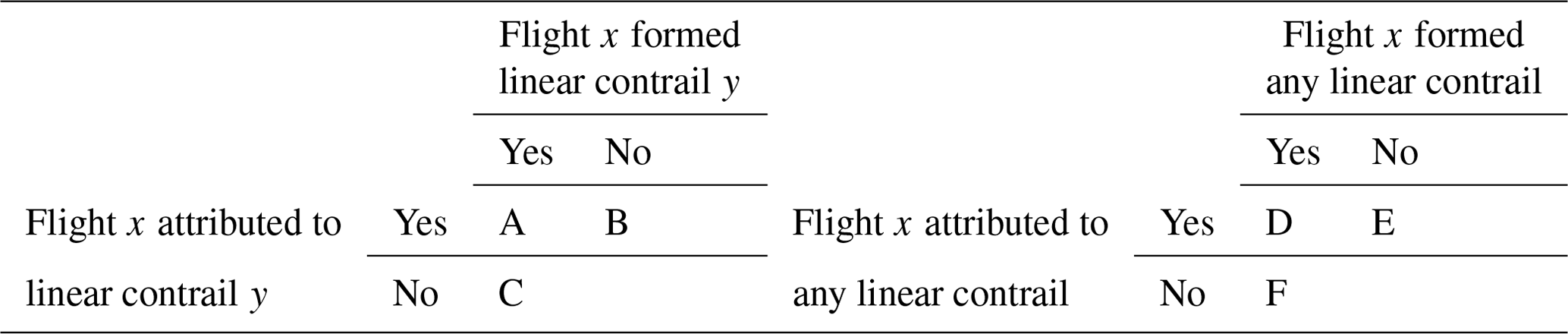
Each metric is composed of cell values from Table 3. The values in each per contrail cell, A, B, and C, are computed by joining each linear contrail in the benchmark dataset with any flight attributions that an algorithm made for that linear contrail. Each linear contrail will have zero or more attributions associated with it. If there are zero attributions, C is incremented. For each attribution, if the flight is the same as the true flight that formed the linear contrail, A is incremented. Otherwise B is incremented. The per-flight-cell values, D, E, and F, are similarly computed by grouping together all linear contrails in the benchmark dataset by the flight that formed them and similarly grouping all attributions by attributed flight. Each flight will then have zero or more linear contrails that it formed and zero or more linear contrails attributed to it. If both are zero, we ignore this flight. If the flight formed linear contrails and there are attributions to it, we increment D. If it formed linear contrails but there were no attributions, we increment F. If there were attributions but it did not form any linear contrails, we increment E.
Once the table is populated, we compute the following metrics. For each, we provide the formula and a prose definition:
-
Contrail precision, A/(A + B). The percentage of the attribution algorithm's attributions to linear contrails that are correct (note that the algorithm can choose not to attribute any flight to a linear contrail).
-
Contrail recall, A/(A + C). The percentage of linear contrails to which the algorithm has attributed the correct flight.
-
Flight precision, D/(D + E). The percentage of flights to which the attribution algorithm has attributed at least one linear contrail that also formed at least one linear contrail in SynthOpenContrails.
-
Flight recall, D/(D + F). The percentage of flights that formed at least one linear contrail in SynthOpenContrails to which the attribution algorithm has attributed at least one linear contrail (regardless of whether that specific attribution is correct).
As (1) there is substantial variation in the properties of the different time spans that might affect attribution performance (see Fig. 4) and (2) we want to avoid the statistics being dominated by the contrail- and flight-dense scenes, we do not recommend computing these metrics uniformly over all of the flights and synthetic contrail detections in the dataset. For the purposes of the benchmark, we compute a central estimate and confidence intervals of the metric value using block bootstrapping (Cameron et al., 2008). Specifically, in each of 1000 iterations, we sample, with replacement, 28 time spans (i.e., the number of time spans in each dataset split) and compute each metric from the union of those time spans. We can then compute the mean, 5th percentile, and 95th percentile from these 1000 measurements.
As the goal is to assess the performance of the attribution algorithms in isolation, these metrics are all computed relative to the filtered and adapted view of CoCiP provided by SynthOpenContrails, and they do not attempt to account for performance relative to the raw CoCiP outputs. This affects the case in which a given flight formed one or more contrails according to CoCiP, but, due to the dataset's post-processing steps, SynthOpenContrails contains no detections of its contrails. If an attribution algorithm were to attribute a synthetic detection to such a flight, it would hurt the per-flight precision and not increase its per-flight recall.
Critically, the flights used to generate SynthOpenContrails are from the same database as those that will be used for the attribution algorithm, but that database is known to be incomplete: at a minimum, military aircraft are unlikely to be fully present, which Lee et al. (2021) estimate to be 5 % of air traffic globally (although this may be higher over our region of study). In order to ensure that the attribution algorithms can handle contrails formed by flights that are missing from the database, we conservatively exclude a fixed random sample of 20 % of flights when tuning and benchmarking. The selection of this value imposes an upper bound on the metrics, which may not be realistic for an MRV system that is run by a government with access to its own military aircraft locations. Because of this, the metrics should not be interpreted directly as the performance of an attribution algorithm in the real world in an absolute sense. They should, however, provide a relative measure of performance between different attribution algorithms. We ran a sensitivity analysis on the impact of excluding different percentages of flights over the attribution algorithm from Geraedts et al. (2024), as well as the CoAtSaC algorithm introduced in Sect. 3. This showed that the recall metrics for both algorithms appear to improve linearly with the fraction of flights available. For the Geraedts et al. (2024) algorithm, the precision metrics were both unaffected by the fraction of flights excluded, whereas for CoAtSaC, the precision metrics improve linearly with the fraction of flights available. While it may be tempting to use the metrics with 100 % of flights available as an absolute measure of performance, this would only hold if the flights missing from the database are a representative sample with respect to contrail formation and attribution performance, which is unlikely to be the case. Therefore, we do not provide the metric values here.
In this study, we benchmark all attribution algorithms using the nominal ERA5 reanalysis weather data, and we recommend that future algorithms evaluating on this benchmark do the same. Using other weather data could result in the improvements over the results presented in Sect. 4 being primarily due to the weather data, rather than the algorithms themselves. As SynthOpenContrails is constructed using data from a weather model, such improvements would not necessarily even indicate the superiority of the weather data when applied to attributing real contrail detections. It is, therefore, also critical that a future attribution algorithm that uses SynthOpenContrails for tuning or benchmarking does not use the same weather data as were used to create the dataset, as specified in Sect. 2.1, because that would provide unrealistically low advection errors.
In this section, we present a novel algorithm for attributing contrails to the flights that created them and demonstrate how it can be tuned and benchmarked using SynthOpenContrails. We call this algorithm “CoAtSaC”, short for “Contrail Attribution Sample Consensus”.
3.1 Data
The inputs to our attribution algorithm consist of linear contrail detections, flight trajectories, and weather data, and they are the same as those used in Geraedts et al. (2024). The spatial regions and time spans used are the same as those for which we generated SynthOpenContrails, as specified in Sect. 2.1.
3.1.1 Contrail detections
When running on real data, we obtain our contrail detections by running the contrail detection algorithm used in Ng et al. (2024) on infrared imagery from the GOES-16 ABI Full Disk product (Goodman et al., 2020). We can alternatively consume the synthetic contrails from SynthOpenContrails as a drop-in replacement that has known ground-truth attribution.
3.1.2 Flight trajectories
We use the same database of flight trajectories provided by FlightAware (https://flightaware.com, last access: 17 July 2025) as was used for generating the synthetic dataset. As we discussed in Sect. 2.5, this dataset is incomplete; therefore, we elide a random sample of the flight data when tuning and benchmarking the dataset on synthetic contrails. We apply the same filtering and preprocessing of flight data as in Geraedts et al. (2024), to filter out erroneous waypoints and those that could not have formed contrails and to achieve a uniform frequency of waypoints across all flights. For each time span of contrail detections, we load flight data starting 2 h before the start of the span and ending at the end of the span, in order to account for the aforementioned delay between contrail formation and detection.
3.1.3 Weather data
The weather data that we use come from the European Centre for Medium-Range Weather Forecasts (ECMWF). For our attribution algorithm, we use the ARCO-ERA5 dataset (Carver and Merose, 2023), which is derived from the ERA5 nominal reanalysis product (Hersbach et al., 2020). This product comprises hourly data at a 0.25° resolution at 37 pressure levels.
3.2 Advection of flight tracks
For the purposes of our contrail attribution approach, we need to answer the following question for each flight waypoint: “Where would we expect a hypothetical contrail formed by the given flight waypoint to appear in a particular satellite scan?”. To answer this, we simulate the advection of each waypoint to each of the subsequent 11 GOES-16 ABI Full Disk images (roughly 2 h at 10 min intervals; see Appendix C1 for the implications of only advecting for 2 h). We again need to account for the GOES-16 ABI capture pattern (see Appendix B2) and compute the expected “scan-time offset” for each waypoint (Meijer et al., 2024). The set of target times for our advection is then the nominal scan times of the 11 scans, with the scan-time offset added. A small amount of error is introduced by the fact that the scan-time offset is not updated as the waypoint advects; if it advects across a capture swath boundary, the scan-time offset would jump by roughly 30 s. The advection itself is performed in exactly the same way as in Geraedts et al. (2024), which we detail in Appendix C2.
This approach to simulating flight advection is subject to a number of sources of error, including (but not limited to) inaccuracies in the interpolated weather data, approximations in sedimentation rate, and not accounting for all physical processes that can affect the vertical location of the contrail (e.g., radiative heating). We expect that these errors will compound over time. As a result, our estimation of where a hypothetical contrail would appear in a particular satellite image will be increasingly wrong as the hypothetical contrail ages, and the errors in successive satellite images will be highly correlated.
Once all flights are advected, we will have advected flights and detected contrails at each satellite frame starting 2 h before the start of a time span and ending 2 h after. This is to ensure that the attribution algorithm can consider flights and contrail detections that are near the beginning and end of the time span in the context of their temporal dynamics.
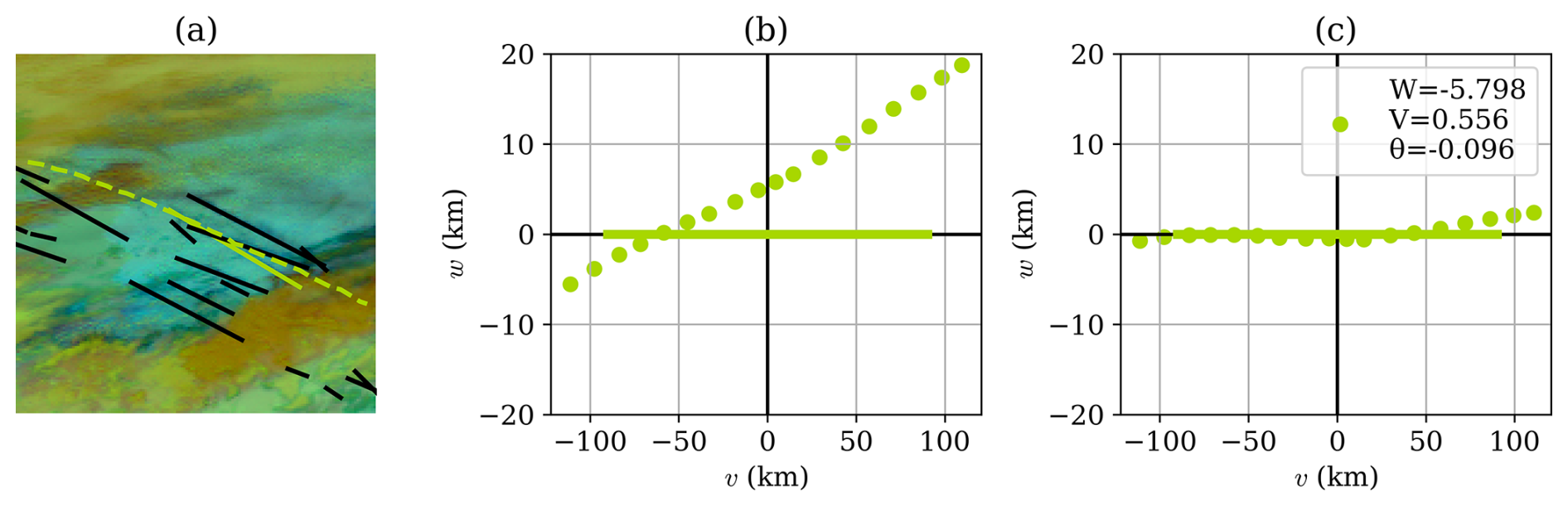
Figure 6A visualization of the single-frame matching process. This is the same scene as in Fig. 1 but focusing in on a single flight and a single contrail detection, rendered in green over a false-color GOES-16 ABI image in panel (a). In panel (b), we show the same data on the v–w plane, with the linear contrail defining the v axis and the flight waypoints projected accordingly to points (wi,vi). Panel (c) shows the results of applying the transformation in Eq. (1) after optimizing the parameters W, V, and θ in Eq. (2), producing points ().
3.3 Single-frame attribution algorithm from Geraedts et al. (2024)
CoAtSaC is an extension of the single-frame attribution algorithm from Geraedts et al. (2024). Here, we summarize just the portions of the Geraedts et al. (2024) algorithm that are critical for understanding CoAtSaC.
The algorithm defines a new 2D spatial coordinate system, which is an orthographic projection centered on a linearized detected contrail, with the v axis along the contrail and the w axis orthogonal to it (we adopt the axis names from Geraedts et al., 2024, but caution the reader not to confuse them with the conventional usage of these variables as directional wind speeds). Distances along each axis are specified in kilometers. Parallax-corrected advected waypoints of a single flight are projected onto this plane to coordinates (wi,vi). Waypoints are excluded if their vi values are outside the span of the contrail, with a small additional tolerance. An example is shown in Fig. 6b.
In this projection, the algorithm measures the advection error that would be implied if this flight formed this contrail, in terms of relative orientation and distance, which are combined into the following coordinate transformation:
The parameters W and V are translation distances along the respective axes and θ is a rotation angle. These parameters are optimized by minimizing the objective function:
which essentially tries to move the flight waypoints as close as possible to the contrail (i.e., v axis), subject to regularization terms. The coefficients Cfit, Cshift, Cangle, and Cage vary with age to allow for a higher tolerance for advection error for flights that have advected longer. The result of the optimization in Eq. (2) is visualized in Fig. 6c, showing both the transformed waypoints and the optimized parameter values. The flight is deemed to have formed the associated contrail if Sattr<3 after the optimization. Section 2.2 of Geraedts et al. (2024) includes some additional logic used to help resolve cases in which multiple flights are attributed to the same contrail detection.
This approach has a few shortcomings that we aim to improve upon. Firstly, an advected flight at a substantially different altitude than the contrail, subject to different wind speeds, could happen to align perfectly in the 2D projection in a single frame as one passes directly above the other at the moment that the satellite captured it. This flight would be erroneously attributed instead of the true flight, which likely incurred some advection error along the way. Secondly, the advection error for each flight segment is treated as independent between satellite frames, when in reality it is highly dependent. We aim to rectify these issues by leveraging the expected behavior of the advection error for the same flight segment as it advects over time.
3.4 CoAtSaC attribution algorithm
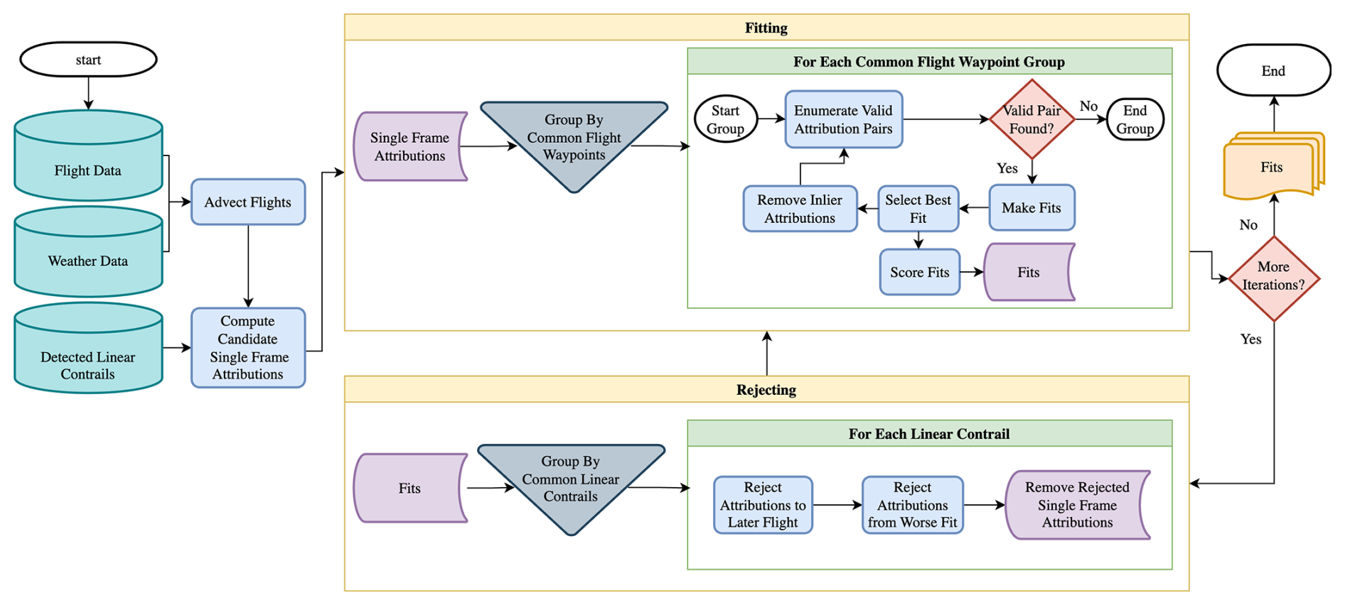
CoAtSaC improves upon the single-frame algorithm by considering the temporal evolution of the transformation parameters V, W and θ from Eq. (1), with a particular focus on W. The algorithm is visualized in Fig. 7. The algorithm is composed of two stages that run alternately. The first stage, called “Fitting”, looks at all single-frame attributions to a single group of consecutive flight waypoints and leverages the expected temporal evolution of W in order to group together detections of the same physical contrail in different frames. The second stage, called “Rejecting”, combines the evidence from the first stage across multiple candidate flights for each contrail detection and uses that to determine a subset of the single-frame attributions which can be confidently rejected. “Fitting” is then run again but without the potential confounders that were eliminated in the second stage. The stages can then continue to be run for more iterations, if desired.
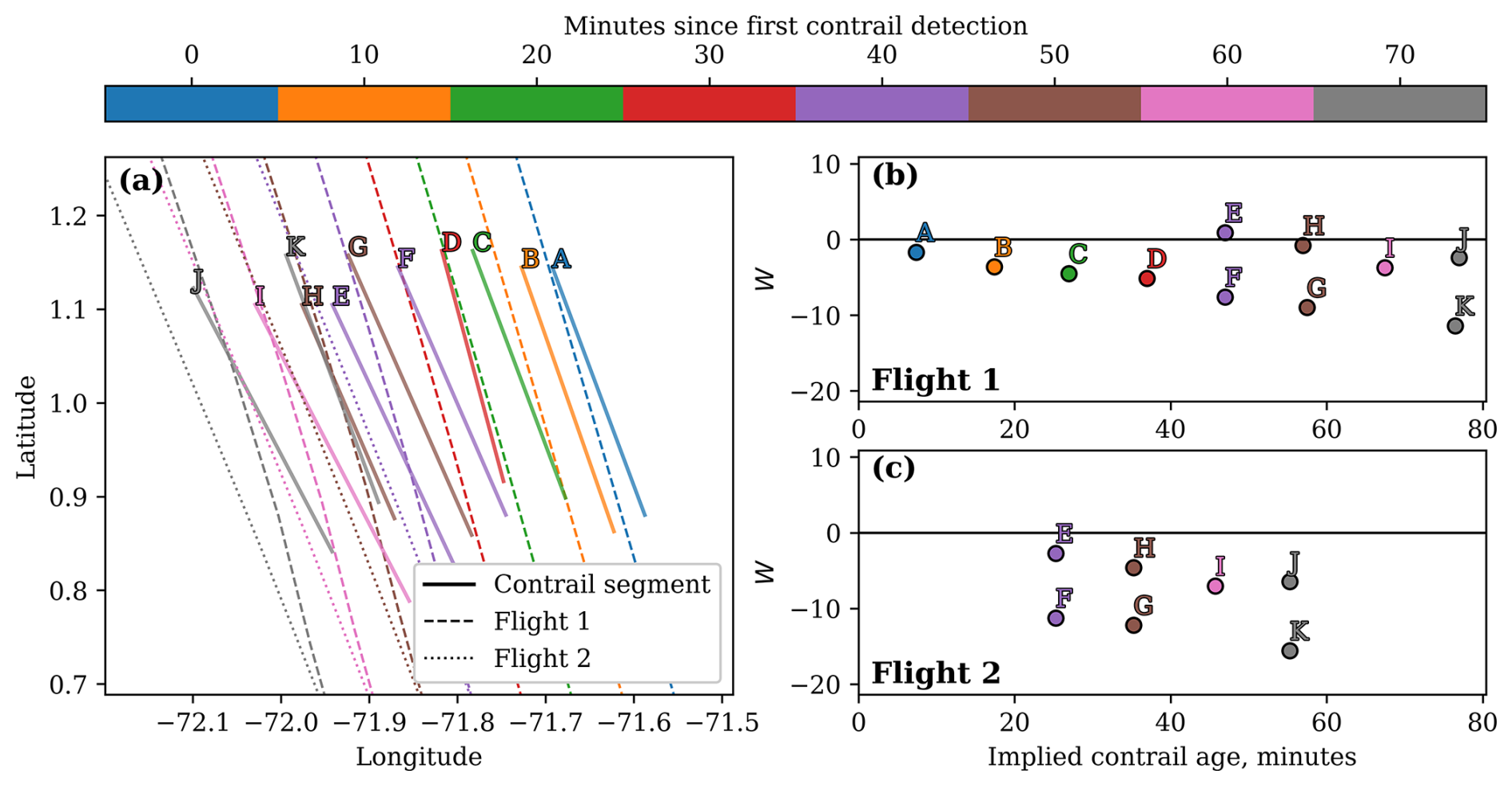
Figure 8Visualization of a contrail-to-flight attribution problem involving two flights that both formed a contrail. Panel (a) shows the detected linear contrails for a 70 min period (covering eight GOES-16 ABI Full Disk scans), accompanied by the flight tracks advected to the GOES-16 capture times. Each linear contrail and flight track is color-coded according to its corresponding satellite capture time. For Flight 1 and Flight 2, in panels (b) and (c), respectively, we show the value of the single-frame attribution parameter W, which approximately measures the advection error perpendicular to the contrail, as a function of the time between the passage of the flight and the moment of detection (i.e., the implied contrail age).
3.4.1 Case study
Before discussing the details of the algorithm, we first present a case study to provide some intuition. We consider the situation in Fig. 8a, which shows two contrails formed by two different flights over a period of 70 min. In Fig. 8a, Flight 1 passes through the domain approximately 20 min before Flight 2 and forms a contrail that is detected in seven consecutive GOES-16 ABI images (line segments A, B, C, D, F, G, and K). The contrail formed by Flight 2 (line segments E, H, I, and J) is first detected approximately 40 min after line segment A is detected. The Flight 1 and Flight 2 flight tracks, advected to the time of each relevant GOES-16 ABI image, are also shown in Fig. 8a as dashed and dotted lines, respectively. Figure 8b and c show the values of the transformation parameter W for each detected contrail for Flights 1 and 2, respectively. For the single-frame attribution algorithm, an ambiguous situation occurs 40 min after the first contrail detection, when line segment E (which is the first detection of the contrail formed by Flight 2) is close to the advected flight tracks of both flights. In fact, Sattr for line segment E is smaller for Flight 1 than for Flight 2 (which is the correct flight). Thus, a single-frame attribution algorithm may erroneously match Flight 1 to line segment E. If, however, we consider the temporal evolution of the value of W for both flights, as shown in Fig. 8b and c, we see that, for both flights, we can identify two sets of single-frame matches, each of which can be connected by a line. For Flight 1, we can imagine points A, B, C, D, F, G, and K forming such a line, while points E, H, I, and J form another line. To understand why this is the case, we note that, for a constant error in the wind data used for advection, we would expect a displacement error between the advected flight track and detected contrail that linearly increases with time, which roughly corresponds to W increasing linearly with time. Importantly, for a flight that formed a contrail, we expect the line connecting the detections to intersect the W axis near zero, implying that if the satellite could have observed this contrail forming, it would be exactly at the location of the flight waypoints before any advection. A contrail that is near an advected flight that did not form it will usually have a nonzero intercept. Considering Fig. 8b, this would lead us to attribute A, B, C, D, F, G, and K to Flight 1 (but not E, H, I, and J). Looking at Fig. 8c in isolation is somewhat more ambiguous, as E, H, I, and J, as well as F, G, and K, form lines with relatively small W intercepts for Flight 2. Only after we also see that Flight 1 forms a line that includes F, G, and K, in addition to A, B, C, and D – some of which formed before Flight 2 had even passed through the region – can we confidently conclude that Flight 2 did not form F, G, and K, but it is the best candidate to have formed E, H, I, and J.
3.4.2 Computing candidate single-frame attributions
The algorithm, based on this intuition, requires access to all single-frame attributions for each flight and the ability to analyze the temporal evolution of the W parameter (Appendix C3 discusses why we do not use V and θ also). For the time dimension of this analysis, as shown in Fig. 8b and c, we use the same “implied contrail age” as was used to set the coefficient values in Eq. (2). Specifically, this is the mean of the advection times of the included waypoints. This “implied contrail age” can vary dramatically for the same contrail detection when attributed to different flights, and the age is in no way inferred from the satellite data directly.
In order to gain access to W values that have a meaningful temporal evolution, we require slight modifications to the single-frame algorithm described in Sect. 3.3. We make the regularization coefficients Cfit, Cshift, and Cangle consistent regardless of contrail age, specifically fixing them at the values they would take on for a flight that had advected for 30 min. We also need to avoid W arbitrarily changing sign across satellite scans for the same flight and physical contrail. For the single-frame algorithm, the sign is unimportant, as the values are always squared in Eq. (2), so making the sign consistent has no negative effect on it. In order to impose consistency, we require that the advected flight be represented with v values increasing with the timestamp of the original waypoint and with positive w values being to the right with respect to the advected flight heading. Specifically, we start from the projected waypoints (wi,vi) described in Sect. 3.3. If the v value for the earliest waypoint is greater than for the latest waypoint, we multiply all of the wi and vi values by −1. For an advected flight segment that is monotonic in v as a function of time, this achieves the desired invariant. Occasionally there are advected flights that loop back on themselves, either due to unusual flight paths or unusual wind patterns, and these can result in inconsistent signs for the w values. We opt to tolerate failures in these cases, as contrails produced by these flight segments are anyway highly unlikely to be successfully attributed, or even detected, by an algorithm based on linearized detected contrails.
We ignore the score thresholds used by Geraedts et al. (2024) and, instead, keep all candidate single-frame attributions whose Sattr score is below a different, tunable threshold, TS, making them available to the “Fitting” stage.
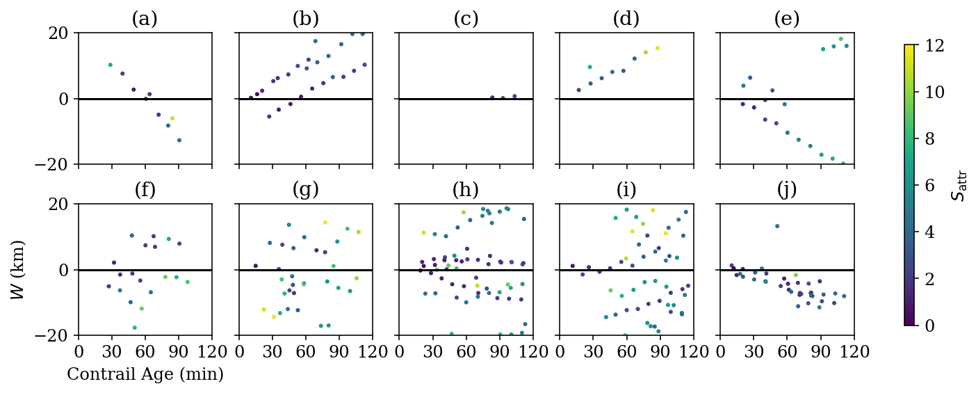
Figure 9Examples of single-frame attributions that share common waypoints of individual flights, plotted on the implied contrail age by W axes. Each single-frame attribution is color-coded according to its single-frame score Sattr. Panel (a) shows two contrails for which the detections at 60 min have a small W value and low Sattr. The single-frame algorithm would incorrectly attribute these detections to this flight; however, because of the large W intercept, we can be confident that they were formed by a different flight. Panel (b) shows three contrails, only one of which was likely actually caused by this flight. Panel (c) presents a contrail with a shallow slope and near-zero W intercept that is first detected long after this flight passed through. This was due to a later flight forming a contrail near the advection path of this flight, but such cases can also be caused by occlusion or small wind shear causing the contrail to remain undetectable for longer. Panel (d) shows a case in which the Sattr values move out of the match range for the single-frame algorithm as the contrail ages, leaving them available to incorrectly match to other flights. Panel (e) presents one long-lived contrail that is likely caused by this flight, with a few other nearby contrails that might make it tricky to fit lines correctly. Panel (f) shows a few short-lived contrails nearby that cause a danger of fitting spurious vertical lines across contrails, unless there is a prior to prefer shallow slopes. Panels (g)–(j) present examples of a higher contrail detection density that result in different degrees of difficulty in identifying the linear structures that track individual contrails.
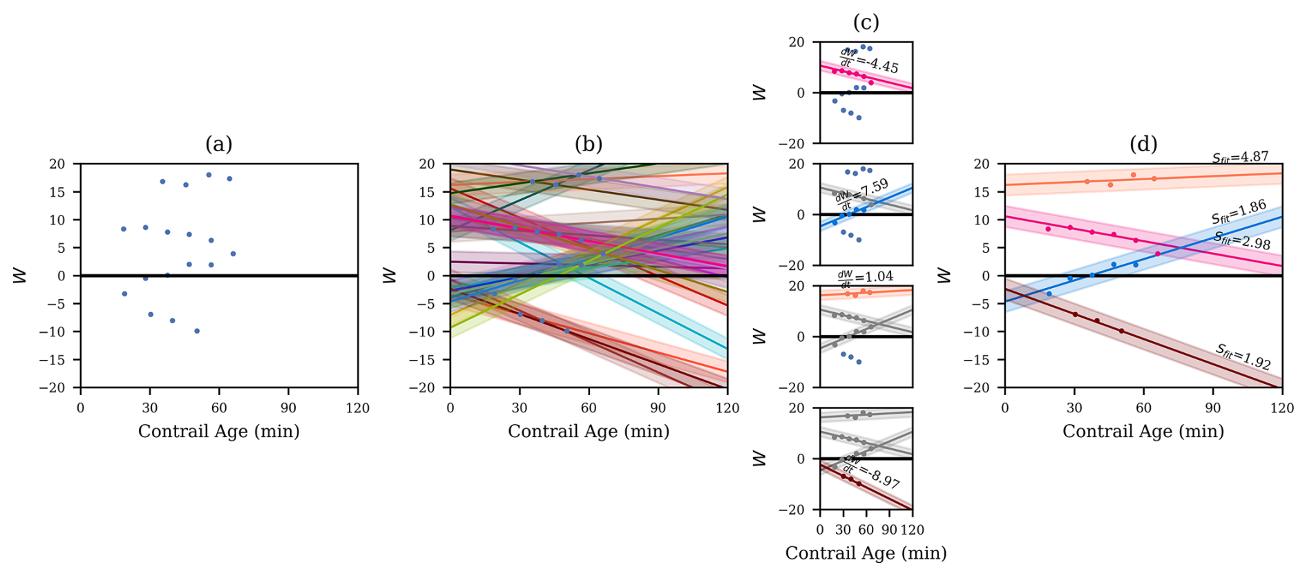
Figure 10A visual depiction of the “Fitting” stage of CoAtSaC for a set of waypoints from a single flight. Panel (a) shows the results of “Group by Common Flight Waypoints” and plots the resulting single-frame attributions in implied age by W space. In panel (b), we “Enumerate Valid Attribution Pairs” and “Make Fits”. In this example, there are 18 single-frame attributions, producing 29 pairs that satisfy the validity criteria. Each of them defines a line, which is plotted in an opaque distinct color, and a surrounding semitransparent region where other attributions would be considered inliers to this fit. Panel (c) shows the “Select Best Fit” and “Remove Inlier Attributions” processes, applied iteratively from top to bottom. In the top panel, we have all fits available, so we pick the best fit, shown in pink, with its slope above it. In the second from the top, we show the first selected fit and its inliers in gray, depicting that we have removed the inliers. We then repeat the process of generating fits from the remaining attributions and selecting the best one, shown in blue. One single-frame attribution would have been an inlier to this fit, but it was claimed by the previous fit, so it is excluded here. The process is repeated until no more candidate fits remain. In this example, four fits are produced. In panel (d), we show the four fits along with their Sfit values produced by “Score Fits”. Note that the orange fit has the highest Sfit score and the shallowest slope, meaning that we are confident that it represents a single physical contrail and also that it was not formed by this flight. Meanwhile, the pink fit has a large W intercept but a relatively low Sfit. The first round of “Fitting” generally has more of these types of fits that will then get removed in the “Rejecting” phase and will not appear in the subsequent rounds of “Fitting”.
3.4.3 Fitting
The intra-flight “Fitting” stage aims to identify groups of single-frame attributions of a given flight that are likely to be the same physical contrail. The stage as a whole is adapted from the Sequential Random Sample Consensus (RANSAC) algorithm (Torr, 1998), which similarly aims to find multiple linear structures among noisy data. An example of this stage is visualized in Fig. 10. The various subroutines of this stage are given a italicized name, for ease of reference to the flow diagram in Fig. 7, and are outlined in the following:
-
Group by Common Flight Waypoints. Having computed candidate single-frame attributions for all flights and all detected contrails, we can now group together candidate single-frame attributions that attribute detected contrails to overlapping sets of waypoints belonging to the same flight. No two resulting groups should contain attributions to the same flight waypoint. The remainder of the fitting stage operates over each of these groups independently.
Within these groups, we can then observe the temporal evolution of W for the single-frame attributions. As we saw in Fig. 8, there is a clear pattern where detections of the same contrail in nearby frames result in a W value that varies linearly in time, even when measured against a flight that did not form the contrail. We show a number of additional examples in Fig. 9, including some where identifying the linear structures is more challenging due to there being large numbers of nearby contrails.
-
Enumerate Valid Attribution Pairs. We enumerate all pairs from the set of attributions in a single group. From each pair, we can then produce a candidate line. We filter out some of these pairs if they do not satisfy the criteria of being temporally within Tt hours of each other, have an absolute slope , and have overlapping attributed waypoints. The slope term, in particular, is important for avoiding fitting lines that span multiple linear structures in the data. If the allowed slopes were unbounded, an example like Fig. 9f could end up with a near-vertical line that groups together what is likely five or six different contrails. This term, in effect, encodes an expected upper bound on the rate of W growth for a contrail. If no valid pairs are found, the Fitting stage is terminated for this group.
-
Make Fits. A pair that passes all of these conditions defines a line, with slope and W intercept Wt=0. The other attributions in the group are labeled as inliers or outliers to this line based on a residual threshold Tres. Specifically, an attribution with implied age ti and W value Wi is an inlier if . This threshold acts as a tolerance for measurement noise that is relatively independent across satellite frames, such as from contrail linearization and quantization of contrail location due to satellite image resolution. Another fairly common scenario that this helps with is if a contrail is detected as a single linear contrail in one frame but is split in two, lengthwise, in the subsequent frame. The attributions to the two smaller contrails would end up with slightly different implied ages than if they were merged, but they likely have the same W value, so the residual allowance enables them to still be inliers. This process of computing fit lines and inliers is shown in Fig. 10b. Hereafter, we refer to the fit line and its set of inliers as a “fit”, and we note that a single-frame attribution can be an inlier to more than one fit at this stage.
-
Select Best Fit. The goal of this subroutine is to identify the candidate fit that is most likely to represent a single physical contrail, irrespective of whether the contrail was formed by this flight. Multiple single-frame attributions attributing a single physical contrail to a flight that did not form it will still form a line, but the line will generally have a nonzero intercept, Wt=0. We do not prioritize finding fits with near-zero intercepts, as it is often easy to spuriously fit a line that spans multiple physical contrails and has a near-zero intercept. Given the set of candidate fits, we select the best fit to be the one with the most inliers. We break ties by selecting the fit with the smallest absolute slope, as steep slopes are more likely to join together different physical contrails, particularly in scenes with many short-lived contrails, like Fig. 9f. The best fit is then stored as an output of the “Fitting” stage.
-
Remove Inlier Attributions. We remove all of the best fit's inliers from the set of candidate attributions in the group. We then return to “Enumerate Valid Attribution Pairs” with the remaining candidate single-frame attributions, repeating until a valid pair cannot be found. This is shown in Fig. 10c.
-
Score Fits. At the end of “Fitting”, we have some number of fits for each group of flight waypoints. Unlike in “Select Best Fit”, where our goal was just to identify fits that most likely represent a single physical contrail, independent of whether it was formed by this flight, we can now make an initial determination of whether the contrail in each fit was likely to have been formed by this flight. To this end, we compute a score as
where is the absolute value of the slope of the fit line; is the absolute value of the W intercept of the fit line; and Cslope, Cintercept, and Csingle are tunable coefficients. This encodes the assumption that a small W intercept, combined with a low minimum Sattr (which primarily helps avoid substantial rotation error) are indicators that the contrail tracked by this fit was formed by this flight. The presence of the slope term is perhaps surprising, as information about the slope was already used in the “Make Fits” and “Select Best Fit” subroutines. The black-box optimizer described in Sect. 3.5 could have set Cslope to zero and did not, but we can only speculate as to why. We hypothesize that it may be due to “Select Best Fit” only considering slope in the context of ties in the number of inliers. In a scene with many short-lived contrails nearby (Fig. 9g, for example), this could produce fits with moderately steep slopes that cut across many physical contrails and, therefore, have more inliers than the fits that only contain a single contrail. The slope term here then allows such fits to have high Sfit values and to, thus, likely be handled by the “Rejecting” phase. The results of the scoring process can be seen in Fig. 10d.
The “Fitting” stage does not itself act on the Sfit score, but a subsequent “Rejecting” stage will consume these scores, and the final time “Fitting” is run, these scores will determine the final attribution decisions.
3.4.4 Rejecting
Whereas the “Fitting” stage uses evidence from one flight at a time to make assessments about which of its single-frame attributions are correct, the inter-flight “Rejecting” stage combines this evidence across flights to eliminate as many incorrect single-frame attributions as possible. Without this stage, there is a strong possibility that the “Fitting” stage would produce fits for multiple flights containing the same contrail detections, all with Sfit scores below the target threshold. This is not inherently problematic, as there can be errors in the contrail detection process that result in merging together distinct contrails. Even when that is not the case, we could express some of the uncertainty in the algorithm by dividing the attribution between multiple candidate flights with different confidences. However, there are cases in which looking across the different flights that have fits containing the same contrail can be used to refine our results.
The existence of the “Rejecting” stage also allows for “Score Fits” to be somewhat more permissive in allowing uncertain fits through to the next stage. For example, in Fig. 10d, the pink fit has an Sfit score just below the threshold that would result in a positive attribution decision, despite having a relatively large W intercept. In most cases, a fit like this is unlikely to result in a correct attribution. In cases of substantial linearization error, however, such a fit can produce correct attributions. Without a “Rejecting” stage the optimal strategy would be to score such a fit above the threshold and not attribute the correct cases. However, by considering further evidence from other flights, the vast majority of the incorrect cases can be ruled out and correct ones can be kept.
The subroutines of “Rejecting”, each given an italicized name to correspond to Fig. 7, work as follows:
-
Group By Common Linear Contrails. The mechanism for combining information across flights is to group together fits produced by the “Fitting” stage that contain attributions to the same detected linear contrail. As fits contain attributions to multiple detected linear contrails, the same fit can end up in multiple such groups.
-
Reject Attributions to Later Flights. The first case of interest is if any pair of fits share at least two contrail detections and if one of them also includes contrail detections that predate the other flight waypoints. In this case, we can assume that the later flight just flew very close to the existing contrail, and we reject the single-frame attributions between the common contrails and the later flight. An example of this can be seen in Fig. 8, where a fit to contrails F, G, and K for Flight 2 might have produced a low Sfit score. Only when we consider Flight 1's fit to A, B, C, D, F, G, and K do we notice that Flight 1's fit includes all of the contrail observations from Flight 2's fit as well as four earlier ones, some of which were observed before Flight 2 even passed through. With access to that information, we can confidently say that Flight 2 did not form this contrail.
-
Reject Attributions from Worse Fit. The second case relies on the quality of the fits produced in the “Fitting” stage. As we saw in Fig. 10, some fits that it produces have W intercepts far from zero, implying a low likelihood that the constituent single-frame attributions are correct. This and other measures of fit quality factor into the Sfit score. Therefore, we compare these values for each of the fits, and if any is more than a threshold Tb higher than the lowest value, we reject all of its single-frame attributions as well. In Fig. 10d, the orange and pink fits, as well as their constituent single-frame attributions, which have W intercepts far from zero, should be eliminated by this process, assuming that the algorithm has access to the flights that did form those contrails.
-
Remove Rejected Single Frame Attributions. The single-frame attributions that were rejected as a result of the two prior subroutines are then removed from the set of candidate single-frame attributions made available to the next iteration of “Fitting”. As more confidently incorrect single-frame attributions get removed, fitting lines to the messier cases – like Fig. 9g–j – becomes easier.
3.4.5 Final attribution decisions
In principle, one could iterate between “Fitting” and “Rejecting” arbitrarily many times, until the algorithm converges. Note that the “Fitting” stage should always be run last. In practice, with the tuned parameter values that we use, there are very few remaining contrails attributed to multiple flights after running just “Fitting–Rejecting–Fitting”. The resulting fits define the final attribution decision for their constituent detected contrails, which is determined by Sfit<3, with the value 3 being chosen for consistency with Geraedts et al. (2024).
3.4.6 Scalability
A critical benefit of CoAtSaC is that it, like the Geraedts et al. (2024) algorithm, is highly scalable. The “Fitting” stage can be parallelized over flights, and the “Rejecting” stage can be parallelized over contrail detections. This lends itself well to being implemented in the Dataflow Model (Akidau et al., 2015) using a framework like Apache Beam (Apache Software Foundation, 2024). In principle, this enables the algorithm to scale to all flights and all contrail detections globally, where the speed of the algorithm is proportional to the number of compute nodes provided to it. This is in contrast to approaches like Chevallier et al. (2023) that optimize over a full graph of flights and contrail detections, which requires holding the complete graph in the memory of a single computer.
3.5 Tuning the attribution algorithm
Given a dataset of synthetic linear contrails labeled with the flight that formed them, divided by time span into train, validation, and test splits, we can then apply it both to tuning and to benchmarking an attribution algorithm. Specifically, we simply run the attribution algorithm using SynthOpenContrails's linear contrails instead of detector-produced contrails and then drop 20 % of flights (as discussed in Sect. 2.5) and compare the resulting attributions to the ground-truth labels that we have for each synthetic linear contrail. From that, we can compute the metrics of interest, as defined in Sect. 2.5.
Using this setup, we apply Google Vizier (Golovin et al., 2017) as a black-box optimization service to search through the space of parameters of CoAtSaC, aiming to find the optimal set producing the highest values for the four metrics of interest using the train split of SynthOpenContrails. We can simultaneously monitor performance on the validation split to ensure that the optimizer has not overfit. How one chooses to prioritize each of the metrics relative to each other – an increase in one often leads to a decrease in another – depends largely on the intended use case for the attributions. If the goal is an MRV system that aims to capture the largest possible fraction of contrail warming – while tolerating some inaccuracies in the specifics – contrail recall might be the most important metric. If one instead aims to generate training data for a contrail forecast model, where noise in the labels could impair the model, flight precision might be the better metric. Using the attributions to evaluate a contrail avoidance trial might require more of a balance between the metrics, depending on the size of the trial. For the purposes of this study, we slightly prioritized flight precision, while keeping the other metrics above reasonable performance thresholds. The parameters chosen by this tuning are given in Table 4.
4.1 Benchmarking attribution algorithms on SynthOpenContrails
We compare the performance of CoAtSaC with the single-frame algorithm of Geraedts et al. (2024) and the tracking algorithm of Chevallier et al. (2023) on the metrics specified in Sect. 2.5 over the SynthOpenContrails test split. Both of the previously published algorithms were slightly modified, as detailed in Appendix D, in order to produce these results, but they were not retuned. Importantly, the tracking algorithm was adapted to operate on the linearized contrails, rather than the contrail instance masks for which it was designed, which may have negatively impacted its performance metrics presented here. Due to time and computational constraints, the tracking algorithm was only evaluated on half of the time spans in the test split, as detailed in Table F3 in Appendix F. This subset is hereafter referred to as the “tracking subset”.
We compute each metric as specified in Sect. 2.5 over the dataset in aggregate, as shown in Table 5, and we also compute them independently per time span in Fig. 11 to give a sense of the variance. We reiterate the caution that these numbers should be interpreted as relative performance metrics amongst the different attribution algorithms: 20 % of flights are artificially excluded in the evaluation, so the upper bound on contrail recall is 80 %, and SynthOpenContrails design choices for outbreak handling and detectable contrail lifetime may influence the metrics.
(Geraedts et al., 2024)(Geraedts et al., 2024)(Chevallier et al., 2023)Table 5Performance of attribution algorithms on SynthOpenContrails (test split) using the metrics defined in Sect. 2.5. Metrics are computed using 1000 iterations of block bootstrapping over the different time spans in the dataset. The metrics are presented as “mean [5th percentile, 95th percentile]“ over the bootstrap samples. Refer to Sect. 3.5 for an explanation of why these should be interpreted as relative performance metrics and may not reflect expected performance in the real world. As Chevallier et al. (2023) could not be evaluated on the full dataset, we report metrics for the other algorithms over the full dataset and then for all algorithms just on the subset of time spans for which Chevallier et al. (2023) could be evaluated. Bold font indicates the best-performing algorithm in each column.
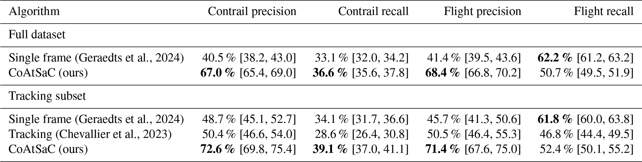
The high-level takeaway is that CoAtSaC outperforms both of the other algorithms with respect to contrail precision, contrail recall, and flight precision, while the single-frame algorithm performs best with respect to flight recall. The tracking algorithm performance appears slightly better than the single-frame algorithm with respect to both precision metrics, but the confidence intervals overlap substantially. Generally CoAtSaC's recall gains are fairly minor, while the precision gains are on the order of 20 % better than the tracking algorithm and 25 % better than the single-frame algorithm. The improvements being far higher in precision than recall is a consequence of the tuning strategy that we used in Sect. 3.5, and we suspect that we could have tuned to higher recall at the expense of precision. It should be noted again here that the weather data selections (see Appendix B1) lead to certain advection error characteristics which (while we have validated them at a distributional level in Appendix B1) could still feasibly (but not necessarily) advantage one or another attribution algorithm on this benchmark in a way that is not representative of real-world performance.
An investigation into the flight recall decrease between the single-frame algorithm and CoAtSaC, seen in Table 5, shows that the flights correctly attributed by the single-frame algorithm but not by CoAtSaC are almost all cases in which a contrail was only detected in a single-frame, which CoAtSaC inherently cannot attribute correctly. We investigated various ways to add handling for single-frame contrails to CoAtSaC, including simply using the single-frame attributions for any contrail detections not attributed by CoAtSaC, but all attempts resulted in substantially lower precision. Of note, SynthOpenContrails may artificially amplify the number of contrails that are detectable in only one frame. Specifically, each time span within SynthOpenContrails defines a 4D box in space and time, and a contrail that advects into the box towards the end of its “linearizable” lifetime or advects out of the box early in its “linearizable” lifetime will only have a single linear contrail in the dataset, despite the fact that it would have been linearized in multiple frames if the boundaries of the space–time box had been shifted. While it is reasonable to assume that contrails that are truly only detectable in one frame have a smaller warming impact than those detected in multiple frames, future research is needed to quantify this.
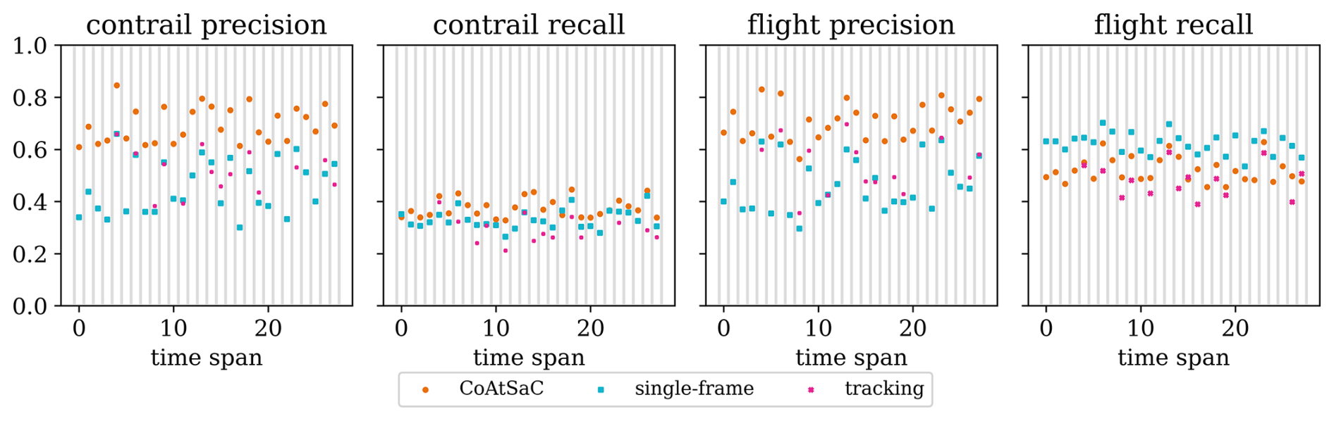
Figure 11The values of each metric computed over each of the 28 individual time spans in the test split, demonstrating the variance in metric values across different scenarios. Note that the tracking algorithm is only evaluated on a subset of time spans.
As the tracking algorithm could only be evaluated on a subset of the dataset, Table 5 includes metrics for all algorithms on just that subset. The fact that the metrics for CoAtSaC and the single-frame algorithm are meaningfully different than those computed over the full dataset is indicative of the variance in performance across time spans. Figure 11 visualizes this variance by showing the metrics computed over each individual time span. This demonstrates the diversity of scenes present in SynthOpenContrails as well as the importance of evaluating on the full dataset. The causes of this variance are further explored in Sect. 4.2.
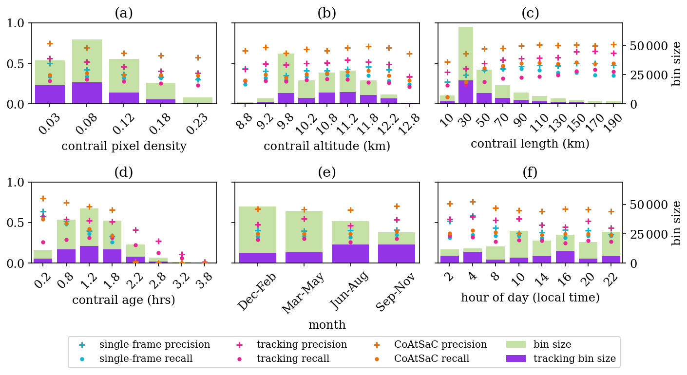
Figure 12Performance metrics of each attribution algorithm shown as a function of various properties available to SynthOpenContrails. The recall and precision used here are contrail-detection-level metrics computed uniformly over the dataset. The green bars show the number of contrail detections in each bin for the full dataset, on which CoAtSaC and the single-frame algorithm were evaluated, while the purple bars indicate the tracking subset. Panel (a) shows performance binned by contrail pixel density (defined as fraction of contrail pixels in the 49×49 pixel window surrounding the center of the contrail). Panel (b) shows performance binned by contrail barometric altitude. Panel (c) shows performance binned by contrail length, as measured along the linearized contrail. Panel (d) shows performance binned by contrail age. Panel (e) shows performance binned by season. Panel (f) shows performance binned by solar hour of the day at the contrail center.
4.2 Performance as a function of contrail properties
Because the SynthOpenContrails contrails are rasterized directly from CoCiP's outputs, we can propagate the properties that CoCiP assigns to each contrail segment through to the final linear contrail instances and then analyze how attribution performance varies with each property. For these analyses, we only look at contrail-detection-level metrics, as many of the properties of interest cannot be meaningfully aggregated to the flight level. We also measure the metrics uniformly across all contrail detections in the dataset, rather than using block bootstrapping, as in the top-level results. Figure 12 shows some examples of performance when computed on subsets of the dataset, when sliced according to various contrail properties. While the relative performance of the algorithms remains quite constant across all of these subsets, the performance for all algorithms falls off with increasing contrail density and age; improves with length; and has more complex relationships with altitude, season, and time of day.
4.2.1 Contrail density
One of the most dominant effects, as seen in Fig. 12a, is that precision and, to a lesser degree, recall decrease with higher contrail density for all algorithms. This is likely also responsible for the seasonal and diurnal effects in Fig. 12e and f, as the higher contrail counts in these cases imply a higher spatial density. It is notable that the special handling for contrail outbreaks in SynthOpenContrails generation substantially influences the density upper bound; consequently, it may have removed many contrails where the attribution algorithms would have exhibited the lowest performance. Appendix E1 discusses how the density effect dominates geographic effects that would otherwise be interesting to study.
4.2.2 Contrail altitude
Contrail altitude also seems to have an impact on the performance of all algorithms, as can be seen in Fig. 12b. As mentioned in Sect. 2.1, the weather data input to CoCiP were inadvertently missing pressure levels between 450 and 975 hPa, which likely caused a small secondary peak of contrails near 6 km altitude, due to the weather conditions for contrail formation and persistence being interpolated down to implausibly low altitudes. We excluded these approximately 1000 implausible contrail detections from this plot to improve the visibility of the remaining data. Within the more plausible altitude bins, there appears to be a trend toward improved performance with increasing altitude up until approximately 11.5 km, after which it then decreases again. It is possible that this is again a contrail density effect, but Meijer et al. (2024) showed that contrail altitudes generally decrease with increasing latitude within this region, and Fig. E1 in Appendix E1 shows that the regions of highest contrail density are in the middle latitudes, so we would expect the opposite effect. Appendix E2 investigates whether the ice crystal radius approximation described in Appendix C2 could be contributing to this effect.
We further investigated the altitude aspects of the incorrect attributions from each algorithm. We observe that very few contrails in SynthOpenContrails are formed below 9.5 km. While all three algorithms attribute a meaningful fraction of contrails to flights cruising below this threshold, CoAtSaC and, to a lesser extent, the tracking algorithm show a substantial reduction in these implausible attributions versus the single-frame algorithm. We see a similar effect when comparing the altitudes of the incorrectly attributed advected flight waypoints to the true altitudes of the synthetic contrails to which they were attributed. We conclude from this that, while CoAtSaC provides a substantial decrease in attributions with large altitude error, introducing an independent altitude signal to the attribution process is nonetheless a promising direction for future work. Further details of this investigation can be found in Appendix E3.
4.2.3 Contrail age
Contrail age is the other axis that seems heavily negatively correlated with attribution performance, as shown in Fig. 12d. The single-frame algorithm has a simple explanation for this, as the Cage term in its score function makes it less likely to attribute a flight to a contrail with a greater implied age. CoAtSaC's behavior is less straightforward. We speculate that it may be tied to contrails growing wider and less linear with age; therefore, the linearization becomes less consistent. For example, if the contrail starts to curve, either the linearization will keep it as a single contrail and join the endpoints, which would likely produce very different W values than when it was more linear, or it could split it into multiple smaller line segments, where the implied ages would vary slightly among the segments, moving them away from the fit line that would join the contrail's detections in its younger, linear phase. This is perhaps an argument for moving towards a more expressive representation of contrail detections, such as instance masks, as used in Chevallier et al. (2023). For the single-frame and CoAtSaC algorithms, the performance artificially goes to 0 at 2 h because flights are only advected for that long; consequently, any detected contrail older than that can only be attributed to incorrect flights. The tracking algorithm allows for longer advection, so it has nonzero performance past 2 h, but both precision and recall decline rapidly with respect to these older contrails. Appendix E4 examines whether similar effects are seen when looking at the total CoCiP-predicted lifetime of the contrail, as opposed to just the age at time of detection. Another potentially age-related effect, the angle between the flight heading and the wind direction, is discussed in Appendix E5.
4.2.4 Contrail length
As shown in Fig. 12c, contrail length has a meaningful correlation with performance, with performance improving monotonically with increased length for all metrics except for single-frame recall. The improved performance with increased length makes sense in the multi-temporal contexts of CoAtSaC and the tracking algorithm, as longer contrails are more likely to persist in multiple satellite frames just due to the time it takes to form them from end to end. As they evolve, they are also likely to produce more stable linearizations and W values over time, due to being better constrained by additional contrail mask pixels and flight waypoints, respectively. The decrease in single-frame recall for longer contrails may be tied to longer contrails generally being less linear, as the wind fields are not uniform over larger spatial regions. Even with a perfectly linear flight path, advection over time can make the contrail nonlinear, but (up to a point) the linearization process will still coerce it into a single linear contrail. This will negatively impact the fit term of Eq. (2), as the rigid transform cannot make a nonlinear advected flight path become linear.
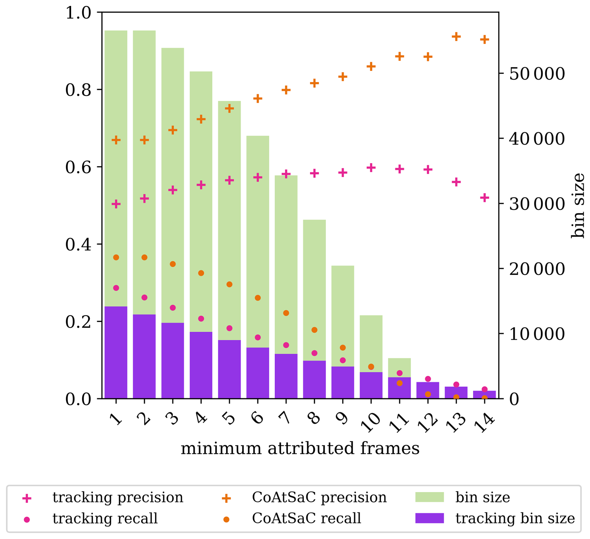
Figure 13The impact on contrail-level precision and recall when only considering attributions derived from observations of a contrail in at least a minimum number of frames. The single-frame algorithm is not presented here, as it does not link attributions across frames.
4.2.5 Attributed frames
Finally, we assess the impact of requiring that contrails be attributed in at least a certain number of frames in order to be considered a match. Both the CoAtSaC and tracking algorithms have a notion of chaining together contrail detections that they assert are observations of the same physical contrail across multiple frames. We hypothesize that those that are attributed in more frames will be higher-confidence attributions; therefore, dropping those attributions with fewer frames would increase precision. As shown in Fig. 13, this largely holds true. CoAtSaC shows a fairly linear increase in precision as the threshold for the minimum number of frames increases, approaching perfect precision at the upper end of the range, but recall decreases quite rapidly. The tracking algorithm shows more modest gains in precision and even reduces somewhat at the high end, but its recall does not decrease quite as rapidly as it does for CoAtSaC. It appears that this could be a valuable lever for an attribution use case that needs very high precision, at the expense of recall.
We have presented a novel, highly scalable contrail-to-flight attribution algorithm for geostationary satellite imagery (CoAtSaC) and a large dataset of synthetic contrail detections (SynthOpenContrails). The SynthOpenContrails dataset allows us to determine that the new algorithm substantially improves upon the previous state of the art. It also allows us to study the performance of each algorithm as a function of contrail and scene properties.
The new attribution algorithm can potentially enable larger-scale live flight contrail avoidance trials, as the methods used to determine contrail formation in previous trials (Sausen et al., 2024; Sonabend et al., 2024) would have difficulty scaling to a larger number of flights. The resulting dataset of flights and contrails could also be used to evaluate contrail forecast models and to train machine learning contrail forecast models similar to Sonabend et al. (2024). In fact, using CoAtSaC attributions in place of Geraedts et al. (2024) attributions indeed improves the primary evaluation metric for Sonabend et al. (2024)'s forecast from 85.5 % to 91.7 %. It is also a necessary step for observational approaches to become a main component of a contrails MRV system or a Scope 3 emissions accounting system.
SynthOpenContrails should be helpful in continuing to improve the state of the art in contrail-to-flight attribution. In particular, it has made clear that there is substantial room for improvement in areas of high contrail density and that entirely different approaches to attribution might be necessary in those settings. It also seems clear that incorporating independent contrail altitude signals in the attribution algorithm has the potential for significant improvement, and future work will be needed to determine how to model those signals in a synthetic contrails context.
When generating synthetic data from CoCiP outputs, we found poor agreement between the CoCiP outputs and our detections. Differences on a per-contrail level are not surprising given uncertainties in weather data (Gierens et al., 2020; Agarwal et al., 2022), but we also found broader qualitative differences, in quantities such as overall contrail density. For the purposes of this study, distributional alignment between the statistics of the synthetic and real contrail detections was sufficient to evaluate a flight attribution system, and we were able to achieve this by introducing variations in detectability as a function of contrail age and density. It would be valuable to disentangle the sources of these qualitative differences, whether they be errors in CoCiP's modeling, errors in the weather modeling, errors in our classification of the subset of contrails that can theoretically be detected in geostationary imagery, or the specific skill of an individual detection model. The answers to these questions could help improve all components of the system, including the detection models, CoCiP and similar physics-based models of contrail formation and evolution, and the weather models themselves. It can also inform which of these components can and should be used in either a predictive or retrospective context for contrail avoidance. One path towards disentangling these questions and validating some of the subjective decisions made in generating the synthetic contrails dataset would be to build a high-fidelity, large-scale dataset of real contrail detections with known flight attribution.
When evaluating an automated contrail monitoring system, one is concerned with the errors from both contrail attribution, which is the subject of this work, and contrail detection, which is not. The methods in this work can only be used to compare different attribution algorithms that operate on the same contrail detections. A useful direction for future work would be a method of measuring the end-to-end performance of the overall detection and attribution system. Observation-based datasets that can track contrails from the moment of formation until they can be detected in a geostationary image (e.g., using ground cameras) could allow this. Because the ultimate goal is the reduction of contrail warming, the fraction of total contrail warming detected by a monitoring system could also be a useful metric. SynthOpenContrails could potentially provide a way to estimate this, as it does simulate the warming of each contrail, and whether that contrail is detectable or not. However, the decisions around detectability in Sect. 2.2 were made with the goal of producing any dataset that qualitatively resembled available contrail detections. We have not established whether the decisions are a unique way of generating plausible detections or how the fraction of warming captured is sensitive to these decisions. We leave this for future work, noting that, for these purposes, observations of contrail warming on a per-contrail basis would be very useful, and radiative transfer modeling, such as in Driver et al. (2025), could also allow for the quantification of detectable warming.
A1 RunCoCiP
Here, we specify the settings that we use for the pycontrails library's (Shapiro et al., 2024) implementation of CoCiP (Schumann, 2012).
In addition to flight track information and weather data, CoCiP requires aircraft performance data, specifically the aircraft wing span, aircraft mass, true air speed, fuel consumption per flight distance, soot number emission index, and the overall propulsion efficiency, which we estimate using the Poll–Schumann model (Poll and Schumann, 2021). The Poll–Schumann model is an open-source point-mass aircraft performance model that estimates fuel flow and other performance characteristics for turbofan-powered aircraft across various flight regimes. It calculates flight performance based on inputs such as the Mach number, aircraft mass, ambient temperature, and aircraft-specific characteristics. To generate the required emission data for the CoCiP model, it incorporates the Fuel Flow Method 2 (DuBois and Paynter, 2006) and the Improved FOX (ImFOX) method (Zhang et al., 2022), in addition to the ICAO Aircraft Engine Emissions Databank.
In order to correct for known biases in ERA5 humidity at cruising altitudes (Agarwal et al., 2022; Meijer, 2024), we further configure pycontrails to use “histogram matching” to scale the humidity values in the weather data to match quantiles of in situ measurements from the In-service Aircraft for a Global Observing System (IAGOS) (Petzold et al., 2015).
We rely on the default pycontrails setting for the maximum contrail lifetime, which is 20 h, although the longest lifetime that we see in our dataset is 13 h.
A2 ReprojectGeostationary
For each flight waypoint that forms a contrail at a given time step, CoCiP models the contrail in a 3D space defined by x, y, and z axes, whose origin is at the advected waypoint location (units are meters). z is the vertical axis pointing from the center of the Earth to the contrail; x points along the horizontal plane orthogonal to z, along the contrail's length; and y is the normal to x in the horizontal plane, with the positive direction to the right of the advected flight heading. Within this space, the contrail cross-section for a given waypoint is modeled as a 2D anisotropic Gaussian in the y–z plane with covariance matrix
To obtain the cross-section parameters at locations between two waypoints, the Gaussian's parameters are interpolated linearly. CoCiP defines the width (B) and depth (D) as
(see Sect. 2.1 of Schumann, 2012, for more details), and it uses that width to compute optical depth properties. In order to render off-nadir contrails in the perspective of a geostationary satellite, we need to recompute these values using the viewing ray of the instrument. Therefore, we compute a vector from each contrail waypoint to the satellite and project it onto the y–z plane, calling it zsat. We then rotate σ such that zsat is now the positive vertical axis and then recompute width, depth, and contrail optical depth from the resulting covariance matrix. This process is demonstrated in Fig. A1.
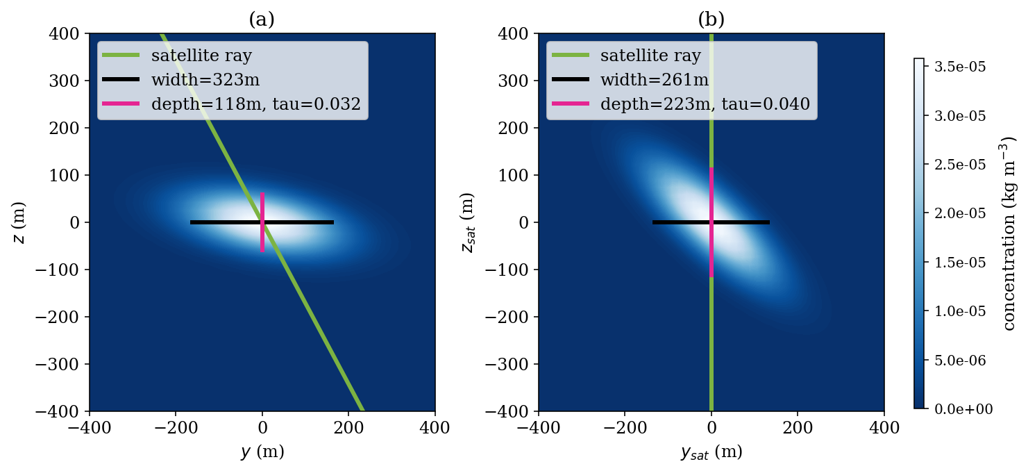
Figure A1A simulated CoCiP plume ice particle concentration profile, placed at latitude 37° N and longitude 120° W, shown (a) in the native CoCiP coordinate system and (b) recomputed from the GOES-16 perspective.
A3 FilterUndetectable
The FilterUndetectable subroutine of the synthetic data generation pipeline aims to compute a detectability mask that filters CoCiP's outputs to just what the Ng et al. (2024) detector would detect. The criteria it uses are as follows:
-
The maximum optical depth of the contrail cross-section at the waypoint must be above a threshold Tτ.
-
As a proxy for other clouds limiting detectability, we require that the CoCiP-reported longwave radiative forcing be above a threshold Trflw.
-
The contrail width must be below a threshold TBmax. This is somewhat counterintuitive, as we generally think of contrails being too narrow to be seen in geostationary imagery. The contrails that are too narrow will be filtered out naturally in the subsequent Rasterize subroutine, so we do not address them here. Here, we are using width as a proxy for linearity. The labelers who labeled the detector training data were instructed to only label line-shaped contrails, because contrails that are past their linear phase are generally challenging to distinguish from natural cirrus. Appendix B4 discusses why it is reasonable to use width as a proxy for linearity for the purposes of detectability.
-
The contrail length must be substantially larger than its width. The labeler instructions in Ng et al. (2024) required that a contrail be 3 times as long as it is wide. To simulate this, we say that a given contrail waypoint will only be detectable if it has a certain number of neighboring waypoints that are also visible according to the previous criteria, where b is the average width of the contrail detection in question, Cl/B is a ratio of flight seconds per meter of width, and CTflight is the number of seconds between flight waypoints after the initial resampling described in Sect. 2.1.1. In order to tolerate small gaps in visibility, we search for the n visible neighbors in a window of n⋅Cndil waypoints in either direction, where Cndil≥1 defines the amount by which we dilate the search window.
As a minor optimization, we qualitatively determined that we most closely match human detectability if we slightly loosen these criteria. Specifically, if a contrail in the given time step has any waypoints that pass all four criteria, we keep all of its waypoints in the contrail that pass criteria 2 and 3. This helps avoid unnatural single-waypoint contrails and hard boundaries that are not due to occlusion.
A4 AdaptToDetector
Here, we detail the adaptations made directly to the CoCiP outputs to better reflect the behaviors of the Ng et al. (2024) detector.
The first is related to condition 3 of the detectability criteria in the FilterUndetectable subroutine (see Appendix A3). We found that using a fixed-width upper bound results in contrails that suddenly disappear in unrealistic ways. In practice there is a decay in the odds of detection as a contrail ages, becoming more dispersed and less linear. As the value that will eventually be rasterized in the Rasterize subroutine is directly derived from optical depth, we simulate this affect by decaying CoCiP's optical depth τ based on both the width and age of the contrail. Specifically we apply the following:
where B is the contrail width in meters and a is the contrail age in hours. This decays τ linearly to zero as the contrail width grows from TBmax−Cdecay to TBmax, and it additionally applies a multiplicative exponential decay based on the contrail age, once it becomes older than Tage hours. See Appendix B4 for further discussion.
The second adaptation is a reflection of how the training data for the detector were labeled. Specifically, the tool that labelers used to draw polygons around contrails did not allow for the polygon to be less than two pixels wide. Consequently, the contrail masks in the OpenContrails dataset (Ng et al., 2024) are never less than two pixels wide, and the detector model learned this behavior, even for contrails that are far narrower than what one would expect for a two-pixel-wide contrail seen in the GOES-16 ABI. To instill this behavior in SynthOpenContrails, we artificially pad the widths (only after all of the aforementioned width-based filtering and adaptation) of contrails whose CoCiP-predicted widths are between Tpadmin and Tpadmax by Cpad.
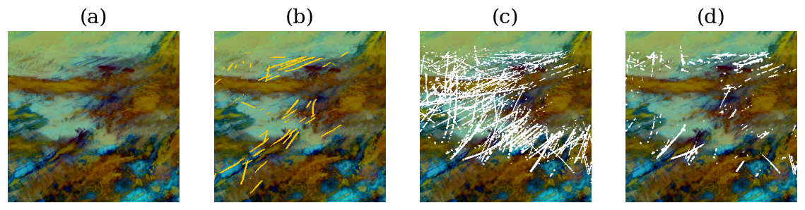
Figure A2A demonstration of the effect of the HandleOutbreaks subroutine. In panel (a), we show an Ash-color-scheme false-color GOES-16 ABI image taken at 22:00 UTC on 11 February 2020, centered just off the coast of Delaware. Many contrails are visible in dark blue, along with some thinner cirrus clouds that may also have originated as contrails. There are also mixed-phase clouds shown in brown that make some contrails difficult to discern. In panel (b), we overlay the detections from Ng et al. (2024) in yellow. In panel (c), we overlay (in white) the results of our synthetic contrails generation before Eq. (A6) is applied. The density of contrail pixels is substantially higher than in panel (b). In panel (d), we show the results of applying Eq. (A6). The density of contrail pixels is much more similar to panel (b).
A5 Rasterize
Here, we detail the process of rasterizing CoCiP outputs in the perspective of a geostationary satellite. This is an adaptation of Appendix A12 in Schumann (2012).
At this stage, we still operate on just a single flight and a single time step. We first parallax-correct each CoCiP waypoint location to the surface latitude and longitude where the satellite would see it. Due to an error, we used the altitude output from pycontrails, which uses an International Standard Atmosphere (ISA) approximation to convert pressure to geometric altitude, for this process, although it would have been more correct to use geopotential to compute it. In Appendix B6, we show that this error is negligible for our purposes. We then map the surface latitudes and longitudes onto the satellite pixel grid but supersampled (Akenine-Moller et al., 2019) to 8 times the true resolution in order to minimize aliasing in the final raster. For each pair (i,j) of adjacent waypoints, with optical depths (, ) and widths (Bi, Bj), we take a square kernel of pixels that includes both waypoints and all pixels that are within max(Bi,Bj) from the segment joining the waypoints. Within this kernel, we look up the latitude and longitude of the centers of each pixel, noting that the grid will be somewhat irregular due to the curvature of the Earth. We then compute (1) the distance s (in meters) from the center of each pixel to the closest point on the segment and (2) the fraction α (this is called w in Schumann (2012), but we want to avoid confusion with other variables of that name here) of the distance along the segment from i to j of this closest point. Following Appendix A12 of Schumann (2012), we can then compute the optical depth of the contrail in this pixel as follows:
Having populated the kernels for each pair of waypoints, we can then combine them back to the supersampled pixel grid, taking a maximum over different waypoint pairs that contribute to the same pixel. We can then downsample to the native satellite resolution and convert to opacity: .
A6 HandleOutbreaks
In principle, the CombineRasters subroutine should produce a final contrail mask, except that this results in certain large areas that are almost entirely marked as contrails; thus, the individual contrails cannot be identified. These are usually in areas where the satellite imagery does exhibit very high contrail density, which we hereafter refer to as “contrail outbreaks”. In the satellite imagery, contrail outbreaks often appear as large areas with amorphous cirrus cloud cover no longer identifiable as individual contrails, other than certain areas of greater optical depth that are still linear. Generally speaking, the Ng et al. (2024) detector will only identify these greater optical depth contrails in outbreak scenarios. It is also likely that the true contrail density is somewhat lower than what CoCiP predicts, as CoCiP does not model the inter-flight effects, where the formation of the first contrail slightly dehydrates the atmosphere, making the next contrail less likely to form (Schumann et al., 2015). As the objective is to simulate the detector's behavior, whether or not CoCiP is overpredicting, we need to modify the outputs in these outbreak areas.
To accomplish this, for each contrail pixel in our mask, we compute a local “contrail density” ρ as the fraction of contrail pixels in the Cσk×Cσk pixel neighborhood that surrounds it. We apply a logistic function
where Cσγ and Cσβ are parameters controlling the rate and domain of scaling applied. We then scale the opacity for that pixel as . This process is demonstrated in Fig. A2.
A7 Linearize
Here, we detail the Linearize subroutine of the synthetic contrail generation process, which takes a single frame of rasterized synthetic contrail opacities and maps them to individual line segments, each representing a single contrail.
First, we reproject our rasterized contrail opacities into overlapping square 256×256 pixel tiles in the Universal Transverse Mercator (UTM) projection, with the UTM zone selected per tile, with a resolution of approximately 500 km of surface distance along each side of the tile. The Ng et al. (2024) detector itself consumes tiles of satellite radiances with exactly the same reprojections applied, in order to avoid many of the distortion issues in the native projection caused by being farther from the satellite nadir. We then threshold the reprojected opacities using , as before. We found that using OpenCV's LineSegmentDetector, as described in Ng et al. (2024), sometimes poorly linearizes wider contrails (both synthetic and real), producing two line segments at either edge of the contrail mask, rather than the desired single line segment in the middle. Therefore, we use the line-kernel convolution-based algorithm described in McCloskey et al. (2021), which is based on Mannstein et al. (1999), for linearizing both the real detector outputs and our synthetic contrail mask tiles. An additional benefit that this approach provides is that this linearization algorithm declares which mask pixels in the tile correspond to each linear contrail that it produces, which allows us to maintain a mapping of the CoCiP output properties contributing to each pixel corresponding to each linear contrail. We then invert the UTM reprojection for these tile pixels to resolve which flights produced the pixels that comprised each linear contrail. In some cases, more than one flight is deemed to have contributed to a single linear contrail, either due to actual contrail overlap or, erroneously, the linearization algorithm. In these cases, we use a winner-takes-all approach and assign the linear contrail to the flight that is responsible for the most pixels. The final step is to deduplicate linear contrails from overlapping regions of neighboring tiles; for this, we exactly follow the process described in Ng et al. (2024).
B1 Use of the ERA5 EDA control run for synthetic dataset generation
In Sect. 2.1.2, we select the ERA5 EDA control run as the weather data to use for generating SynthOpenContrails. We note that the control run is not simply a lower resolution of the nominal product, as the full EDA spread is used to set bias terms of the data assimilation process in computing the ERA5 nominal data (Hersbach et al., 2020). The important characteristic of the weather used for the dataset is that the differences, or error, between it and the weather used for advecting flights for the attribution algorithm (the ERA5 nominal product is used for all algorithms evaluated in this study) be comparable to the error between the weather used for attribution and reality. For our use case, we are primarily concerned with the subset of weather error characteristics that contribute to advection error, which is substantially narrower than the full set of possible weather data errors.
One way to measure this error is to look at the distribution of W values from the single-frame attribution optimization outputs (regardless of final attribution determination) between flights advected with the ERA5 nominal product and real detected contrails and to compare it to the distribution of W values for the same advected flights computed against synthetic contrails generated (as described in Sect. 2) with particular weather data. If the distributions match, the error characteristics are likely close enough for our purposes. We applied this test, using ERA5 nominal data to advect flights and the ERA5 EDA control run for generating synthetic contrails. The distribution of W values for the real contrails has a standard deviation of 15.0 km, while this value is 15.2 km for the synthetic contrails. The distributions are plotted in Fig. B1. We acknowledge that matching the W distribution does not capture all components of advection error – in particular, the spatiotemporal error covariances may still differ – and the fact that the EDA control run shares an underlying model with the ERA5 nominal product increases the likelihood that this is the case. Further research is required to determine (and maybe generate) a source of weather data that exactly matches every relevant characteristic of this error: perturbing only the wind field may result in physically implausible or inconsistent atmospheres and could be counterproductive to the goal of generating well-matched error characteristics. It is possible that recent advances in machine-learned generative diffusion models being applied to ensemble weather generation (Price et al., 2025) could generate well-matched error characteristics. We expect that this will become more necessary as attribution algorithms start to approach perfect accuracy.
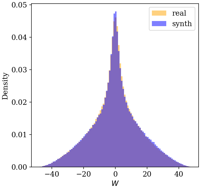
Figure B1The distribution of W values for all flight and contrail pairs in the validation time spans that produce an Sattr value of less than 12. The real contrail detection distribution is shown in orange, whereas the SynthOpenContrails distribution is shown in blue. The distributions are nearly identical.
B2 GOES-16 ABI scan-time offsets
Figure B2 shows the time interval between the nominal scan start time for the GOES-16 ABI and when each pixel is actually captured. The disk is divided into 22 west-to-east swaths, which are captured from north to south over the course of 10 min. This needs to be taken into account when advecting flights for the purposes of contrail-to-flight attribution, as advecting to the nominal scan start time can introduce substantial error relative to when a detected contrail was actually captured. It similarly needs to be accounted for in synthetic contrail detection generation in order to determine the contrail location and properties at the correct times when the satellite would have captured it.
B3 Advection time error in synthetic dataset generation
In the RunCoCiP subroutine in Sect. 2.2, we configure CoCiP to provide outputs on 30 s intervals and map the true satellite capture time to the nearest CoCiP output time, which is a maximum of 15 s away. At 75 m s−1 wind speeds this would incur 1125 m of advection error, which is only slightly more than half of the GOES-16 ABI nadir resolution. We measured the distribution of ERA5 EDA control run wind speeds experienced by all flights in the dataset and found that 75 m s−1 is more than 3 standard deviations (SDs) above the mean (mean =25.3 m s−1, SD =15.7 m s−1). Even the maximum wind speed in the dataset (103 m s−1) results in subpixel error. Therefore, we consider this error to be negligible for the purposes of our analysis.
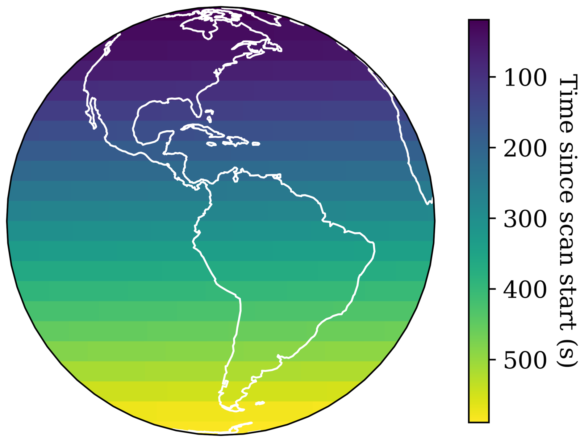
Figure B2Scan-time offsets (the number of seconds after the nominal scan start time) for locations on the GOES-16 disk, when using the Scan Mode 6A (the current default scan pattern).
B4 Width and age decay of synthetic detectability
In both the FilterUndetectable and AdaptToDetector subroutines of the synthetic dataset generation described in Sect. 2.2, CoCiP's predicted contrails growing very wide is interpreted as a proxy for the contrails becoming undetectable. Additionally, in Eq. (A4) in Appendix A4, contrail age being over a threshold is multiplicatively applied as a further decay of detectability. The justification for this lies in how CoCiP makes some simplifying assumptions that certain physical processes can be partially or totally ignored because they apply only at smaller spatial scales than the contrail plume, whose cross-section CoCiP requires to be Gaussian. One of these processes is sub-grid-scale (SGS) turbulence. CoCiP takes SGS turbulence into account only as a factor that slightly increases the rate of ice particle loss, which is then applied uniformly across the contrail cross-section, leading to a decrease in optical depth and total contrail lifetime (Sect. 2.12 of Schumann, 2012). While this assumption of applying the effects of SGS uniformly across the contrail may be fine for CoCiP's own purposes, it creates a challenge for the purposes of detectability, particularly when the contrail is wide enough to span multiple satellite pixels: nonuniformity in rates of ice particle extinction across the contrail would result in local variation in optical depth. This could manifest as irregular widths, gaps, and deviation of the width-wise center of the contrail away from the advected waypoint location, all of which would contribute to becoming undetectable, and none of which are modeled by CoCiP. The width-based decay is introduced here as a simplified model of detectability loss due to these processes.
There are other approximations that CoCiP makes that likely also affect detectability. Because, by definition, SGS turbulence cannot be directly read from the weather model, its magnitude is inferred to grow quadratically with wind shear (Eq. A20 of Schumann, 2012), as derived from the Richardson number. CoCiP does not directly compute wind shear from the weather model data either; instead, it applies an enhancement factor (Eq. 39 of Schumann, 2012), which is a function only of contrail depth, to what would be computed directly from the weather data. This enhancement is inspired by Houchi et al. (2010), and it notably results in matching radiosonde shear measurements at a distribution level but not in the specifics. In CoCiP, a contrail's width increases with age as a function of primarily both wind shear and vertical diffusivity (Eq. 29 of Schumann, 2012). Vertical diffusivity is also a function of turbulence, but CoCiP uses a fixed value for turbulence in this case (Eq. 35 of Schumann, 2012). Taken together, all of these simplifying assumptions, coupled with the relatively low spatiotemporal resolution of the weather data, result in the CoCiP contrails growing wider at a relatively uniform rate along the length of the contrail, when in fact there should often be more variation. This effect compounds with contrail age and is not strictly dependent on contrail width; therefore, the age-based decay aims to capture this effect.
B5 Beer–Lambert law applicability
In the Rasterize subroutine of Sect. 2.2, we apply the Beer–Lambert law (Beer, 1852) to map CoCiP's optical depth to opacity, κ, which is then directly rasterized and thresholded to determine a final synthetic contrail mask. CoCiP's optical depth is computed at a 550 nm wavelength, whereas the bands that the detector uses are in the thermal infrared range (8.5–12 µm). Per Schumann et al. (2012), the absorption optical depth in the thermal infrared range is approximately half of the 550 nm optical depth. Because the final mask will be determined by thresholding κ, this mismatch will simply result in a different threshold value being used. We find it reasonable to apply the Beer–Lambert law here, despite contrails not being a purely absorbing-medium, as the contribution of scattering to the optical depth of high ice clouds is negligible in the thermal infrared bands when compared to that of absorption (Jin et al., 2019). This would not hold if shortwave bands were used for detection.
B6 Barometric altitude conversion
We analyzed the impact of applying parallax correction of advected flight waypoint locations relying on International Standard Atmosphere (ISA) approximations for converting pressures to geometric altitudes rather than using geopotential heights to be more precise. We took the pycontrails outputs for each waypoint at each time step where it contributed to the final contrail masks in the SynthOpenContrails validation set. We measured the Euclidean distance in the GOES-16 ABI's native resolution for infrared bands between the subpixel location that the waypoint would project to using the ISA altitude and the geopotential height. We found the mean distance to be 0.200 pixels and the standard deviation to be 0.066 pixels. This suggests that the error it contributes is likely negligible for the purposes of SynthOpenContrails (and likely also more generally for the class of contrail-to-flight attribution in geostationary satellite imagery algorithms considered in this study).
C1 The 2 h advection
The decision to advect flights for only 2 h could limit the performance of the attribution algorithm. Many contrails do persist and remain detectable in the GOES-16 ABI for longer than 2 h (Vázquez-Navarro et al., 2015, showed this for the Meteosat Second Generation satellite's SEVIRI instrument, which has a lower spatial resolution than the GOES-16 ABI has), and this decision makes it impossible to attribute these older observations properly, as the correct flight will not be available to the attribution algorithm. Driver et al. (2025) found that virtually all GOES-16 ABI detectable clear-sky contrails will become so within the first 2 h of their lifetime. This implies that, if the goal of attribution is to determine whether a contrail formation forecast, like what was used in Sonabend et al. (2024), was correct for a given flight segment, 2 h advection is usually sufficient. While CoAtSaC is benchmarked at 2 h advection, it is technically duration-agnostic. Beyond 2 h, however, we see a slight decrease in attribution performance, likely due to increasing the number of candidate flights involved in the attribution decision for each observed contrail.
C2 Advection algorithm
We simulate the advection of flights in 3D using the third-order Runge–Kutta method (Bogacki and Shampine, 1989) with winds linearly interpolated from the weather data. Similar to Geraedts et al. (2024), we assume an initial wake vortex downwash of 50 m and additional altitude loss due to sedimentation of the contrail's ice particles over time. In order to correctly compute sedimentation rates, we would need to know the relative humidity along the advection path, but the ERA5 relative humidity values at flight cruising altitudes are known to be unreliable (Agarwal et al., 2022; Meijer, 2024). As one of our goals with contrail attribution is to evaluate contrail forecast models, most of which require relative humidity as an input, we want to avoid the attributions that we produce having correlated errors with the forecasts, so we do not use relative humidity for computing sedimentation rates. Instead, we follow Geraedts et al. (2024) and sediment the contrail at a rate that is purely a function of contrail age based on a statistical fit to model data from Schumann (2012), which we would expect to be approximately correct on average but not necessarily in the specifics.
C3 Rationale for not using transformation parameters V and θ
The CoAtSaC algorithm presented in Sect. 3.4 focuses specifically on the W parameter of Eqs. (1) and (2), but it only indirectly consumes the V and θ values by way of thresholding the single-frame Sattr values and incorporating Sattr into Eq. (3). Here, we discuss why the advection errors implied by V and θ carry less signal than that of W for the purposes of providing a signature useful for contrail-to-flight attribution.
The problem with V is that, if there is substantial error in the v direction (parallel to the contrail), it manifests as changing the set of advected flight waypoints that are determined to be overlapping the contrail and are then input to Eq. (2). This is tricky to resolve, as the contrail detections available at this stage are linear by construction, and most advected flight paths are also quite linear, so there are very few features to assist with proper alignment. A tracking-based approach, similar to Chevallier et al. (2023), that directly consumes a contrail pixel mask or even raw radiances could potentially align features of the detected contrails across frames, potentially also better aligning with any nonlinearities in the advected flight path, to help minimize this drift in waypoint overlap.
The parameter θ also appears not to have much signal. We speculate that this is due to θ being a second-order effect, as it measures the change in advection error in the w dimension over the length of the contrail. This measurement is made noisy by the varying lengths of contrails and the fact that they are often short relative to the spatial resolution of the weather data. Specifically, as can be seen in Fig. 5, 21 % of detected contrails have lengths shorter than the 31 km average grid size of the ERA5 weather data, and 59 % are shorter than 62 km. This implies that variation in advection errors across a flight segment matching to shorter contrails will be dominated by the effects of the interpolation scheme in the weather data, whereas more of the variance will be due to inherent errors in the weather data for longer contrails.
D1 Changes to the single-frame algorithm
For the single-frame algorithm, we evaluate the original parameter values specified in Geraedts et al. (2024) and do not retune using SynthOpenContrails. One notable difference in our implementation of the single-frame algorithm, both in how it is used on its own and how it contributes to CoAtSaC, is that Geraedts et al. (2024) split flights up into 10 min segments and computed attributions independently per segment, whereas we chose to apply the algorithm over full flights. This avoids edge effects on segment boundaries, and we find that it improves the results of the single-frame algorithm slightly.
D2 Changes to the tracking algorithm
For the tracking algorithm in Chevallier et al. (2023), we made the following changes for compatibility with the SynthOpenContrails. The advection method used was a reimplementation of that used in Geraedts et al. (2024), using ERA5 nominal data on pressure levels. The tracking algorithm was designed to operate on contrail instance masks, which is not an explicit output of SynthOpenContrails. It does implicitly provide something similar, as the Linearize subroutine already calculates a set of mask pixels that it believes correspond to each linearized contrail, but these were still qualitatively quite different from the instance masks used in Chevallier et al. (2023). Therefore, we slightly adapted the tracking algorithm to operate directly on the linearized contrails provided. This makes it more comparable with the other algorithms used here but limits its performance somewhat. A future goal is to adapt SynthOpenContrails to emulate an instance segmentation model, as opposed to the global segmentation model emulated in the current approach. The parameters of the algorithm were otherwise kept exactly the same as in the original paper, although they were originally tuned for the GOES-16 ABI's Scan Mode 3, which provided an image every 15 min, and SynthOpenContrails uses the current Scan Mode 6a, with data every 10 min. Future work should use the training and validation splits of SynthOpenContrails to further tune the parameters of the tracking algorithm. In Chevallier et al. (2023), the results are presented by applying a threshold on the minimum lifetime of the detected contrail, with the expectation that this improves precision. Here, we present all results without that filter. The impact of that decision is discussed in Sect. 4.2.5 and Fig. 13.
E1 Geographic slicing
Figure E1 shows the performance of each benchmark metric binned by geographic region, along with the number of synthetic contrails in each bin. The effect of contrail density is so dominant here that it makes it very difficult to answer some other questions using these data. For example, does the performance degrade with decreasing spatial resolution as you approach the edge of the disk that the satellite captures, perhaps due to increased error in the position of the detected contrails? In the region of interest for this study, with the GOES-16 ABI, this would be seen in the northwestern United States and Canada, in the upper-left corners of Fig. E1. However, what we see is that this region also has an above-average contrail density. Consequently, further investigation is required to disentangle these effects. There may, nevertheless, be other geographic performance biases that can be explored with these data.
Figure E1Contrail-detection-level performance metrics of each attribution algorithm binned geographically by Level 7 S2 Geometry (Google, 2024) cell within the analysis region, rendered from the GOES-16 ABI perspective. Note that the bin sizes are the same for the CoAtSaC and single-frame algorithms, as shown in the “contrail count” plot, but the “tracking” algorithm is only evaluated on a subset of the data, so its bin sizes are shown separately, using a different scale.
Figure E2Plots in the same style as Fig. 12 but binning by some additional properties. Panel (a) shows performance binned by total lifetime of the contrail that was detected, as predicted by CoCiP, which is not the same as its detectable lifetime. Panel (b) shows performance binned by the cosine of the wind direction relative to the flight heading for the true flight that formed the contrail. Panel (c) shows the performance binned by the difference in contrail ice crystal radius between what CoCiP predicts and the prediction from the statistical function of age mentioned in Appendix C2. The “tracking” algorithm is not plotted here, as we do not have access to its approximation.
E2 Ice crystal radius error slicing
It stands to reason that the performance varying with altitude, as discussed in Sect. 4.2.2, may be due to the ice crystal radius approximation error (see Appendix C2), which we see (in Fig. E2c) has a strong correlation with benchmark performance for CoAtSaC and the single-frame algorithm. Specifically, if the ice crystal radius approximation error correlates with altitude, this would lead to sedimentation rate errors and, thus, advection errors, which also correlate with altitude. We in fact see this correlation in Fig. E3, where the mean error decreases with increasing altitude. However, we do not see the crystal radius error going back up at the higher altitudes, so it does not explain the attribution performance decrease there. The tracking algorithm uses a similar – but not identical – method for approximating ice crystal radius to the other two algorithms but, nonetheless, shows the same general altitude effect.
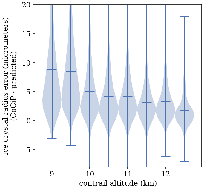
Figure E3A violin plot showing the distribution of ice crystal radius error between what CoCiP predicts and the predictions from the statistical function of age mentioned in Appendix C2, binned by contrail altitude. The horizontal lines indicate the mean of the distribution.
It may be tempting to conclude that Fig. E2c and Fig. E3 taken together indicate that the approximation of ice crystal radius used in the both the single-frame and CoAtSaC algorithm is detrimental. It is important to point out, however, that this is a comparison to the “ground truth” that is generated from reanalysis data, and the entire purpose of the age-based approximation is that these data are known to have inaccuracies, so matching the “ground truth” exactly would not necessarily translate to better performance on real data, but it would trivially improve performance on SynthOpenContrails. Further study is needed to characterize this component of the error and whether something is needed beyond just using different ERA5 EDA members in order to make a synthetic dataset better able to model true sedimentation rates.
E3 Altitude error
Figure E4 provides further visibility into how altitude factors into each algorithm's results. Figure E4a shows the ground-truth distribution of contrail formation altitudes in SynthOpenContrails, binned by flight levels, defined as a barometric altitude measured in hecto-feet (1 hecto-foot corresponds to 30.48 m). Note that flights in North America generally cruise at intervals of 10 flight levels. The top panel shows the overall distribution and the lower panel shows the tracking subset. Each bin is overlaid with the fraction of contrails in the bin that each algorithm attributes correctly. There is no substantial difference in performance between flight levels for any algorithm, and the differences between algorithms reflect the dataset-wide contrail recall differences. We observe that essentially all of the contrails are formed above flight-level 300, and those few that are not are likely due to the aforementioned weather interpolation error. There is also an alternating effect in bin size between “even” (multiples of 20 flight levels) and “odd” flight levels, where the even flight-level bins are generally substantially smaller than their neighboring odd-flight-level bins. Within North America, the even flight levels are assigned to flights heading south or west, while the odd flight levels are assigned to flights heading north or east. This may indicate different rates of producing detectable contrails based on the degree to which the flight heading is aligned with the prevailing winds, although we note that this effect is not seen in Fig. E2b in Appendix E5. Further study is needed to explain this phenomenon and to understand if it is also present in real data or is an artifact of CoCiP.
Figure E4b shows the distribution of flight levels for the segments of each flight that are incorrectly attributed to contrails. These again look fairly similar across algorithms. We note, however, that all three have nontrivial numbers of attributions to flights below flight-level 300. The single-frame algorithm has the highest rate (at 10.5 %), followed by the tracking algorithm (with 7.8 %) and CoAtSaC (with 7.1 %). This demonstrates that incorporating the temporal dynamics into the attribution can reduce these seemingly implausible attributions.
Figure E4c looks at the altitudes at the time of contrail observation, rather than formation. Specifically, it again looks only at the attributions to incorrect flights, and it subtracts the ground-truth altitude of the center of the contrail at the time of observation from the altitude of the incorrectly attributed flight segment after simulating its advection. All of the algorithms show a fairly widespread, indicating that adding an external signal for observed contrail altitude could help substantially, even without perfect accuracy. The secondary peaks, especially visible in the single-frame distribution, are likely tied to the flight-level quantization of the original flight tracks. In the single-frame results, we can identify the peaks corresponding to three flight levels in each direction, whereas the other two algorithms only clearly show one in each direction. This is, again, likely a result of incorporating temporal dynamics, as the likelihood of having the same wind speed at different flight levels may decrease with increasing distance between the flight levels. We further observe that the distributions are asymmetrical. In 9.2 % of the single-frame algorithm's incorrect attributions, the true contrail altitude is more than 2 km above the advected flight, although this value is only 3.8 % in the reverse direction. The tracking algorithm is 6.7 % versus 2.1 %, whereas CoAtSaC is 4.5 % versus 2.2 %. Generally, this shows that slightly fewer of CoAtSaC's errors are at substantially incorrect altitudes, which is again attributable to wind speeds being more correlated at nearby altitudes. The asymmetry is likely a result of contrails forming near the upper range of commercial flight cruising altitudes, which provides a relatively small upper bound on how far above a contrail an incorrectly attributed advected flight can be, but there is a much wider range of altitudes available for incorrect attributions lower than the contrail.
E4 Contrail lifetime slicing
Figure E2a slices performance based on the total CoCiP-reported lifetime of the detected contrail. The units here are still contrail detections, so detections of the same contrail will appear in the corresponding histogram bin multiple times, and the longer-lived contrails presumably appear more times. However, this is artificially flattened out by the age-based decay of optical depth in Eq. (A4). If we ignore the first bin, which is nearly empty, Fig. E2a is just a stretched out version of the contrail age slicing in Fig. 12d.
E5 Relative wind angle slicing
We investigated the hypothesis that the relative angle between the flight heading and the wind direction impacts attribution performance. This was motivated by the fact that contrails that are advecting directly along the original flight path are difficult for humans to attribute in most existing visualization methods. Furthermore, given that the advection is almost entirely in the v direction (as in the v–w plane, not the conventional u–v wind direction vectors), this could hurt an algorithm dependent on wind error only in the w direction. As we show in Fig. E2b, none of the algorithms seem to suffer in this scenario. Performance on some metrics is actually slightly higher when the flight is flying directly into or along with the wind, as opposed to perpendicular to it. Perhaps the more interesting property to study would be the direction of wind shear relative to the flight heading, as it would directly impact the rate of contrail width increase; however, unfortunately, pycontrails does not currently provide that information.
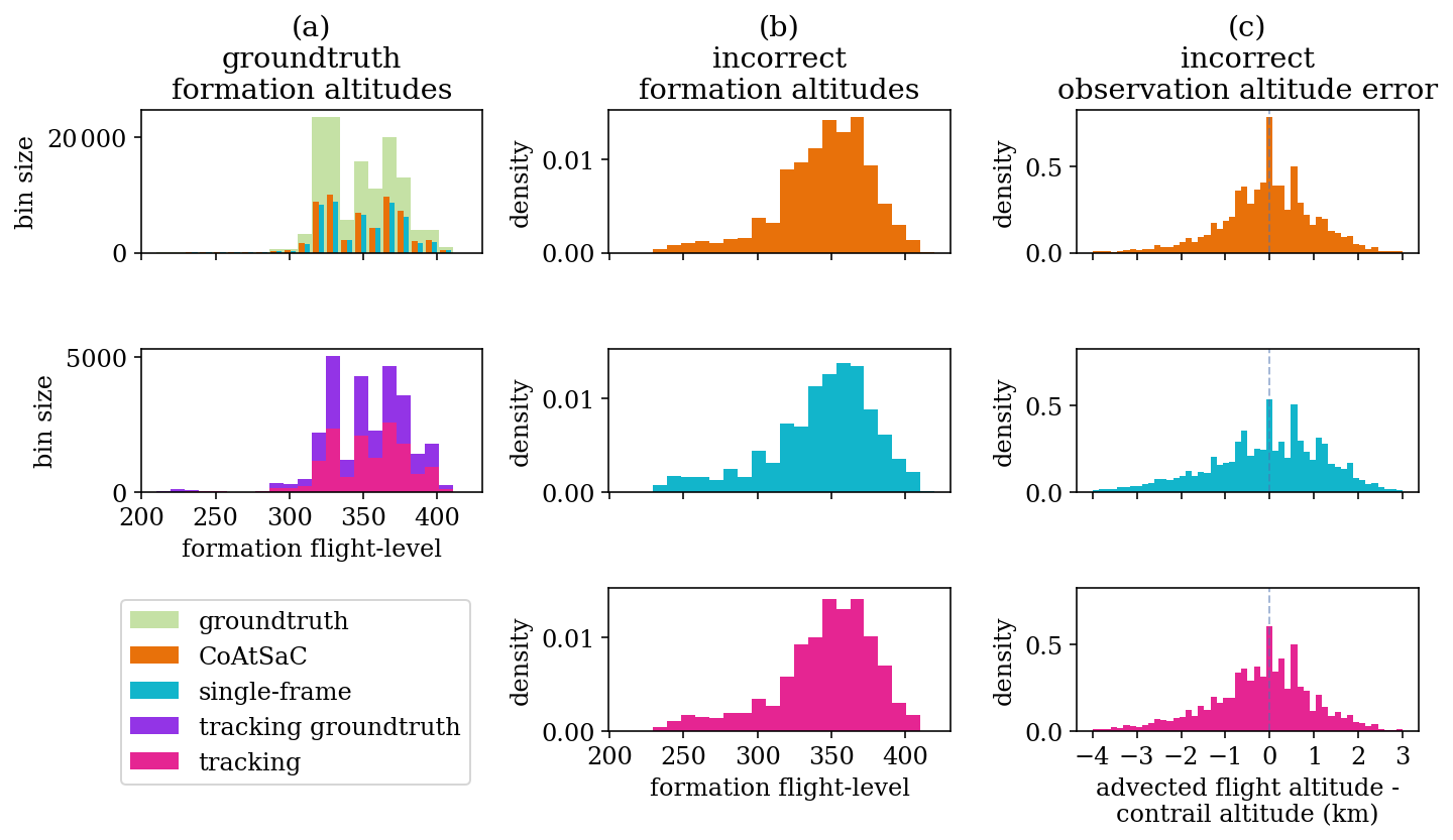
Figure E4Altitude-related distributions of the attributions from all three algorithms. In panel (a), the top subpanel shows the distribution of flight levels at which the SynthOpenContrails contrails were formed (in green), weighted by the number of frames that each contrail is detected in. The orange and blue bars show the fraction of contrail detections from each bin that are correctly attributed by the CoAtSaC and single-frame algorithms, respectively. The lower subpanel shows the flight-level distribution of the subset that the tracking algorithm was evaluated on (in purple) and the fraction of each bin that the tracking algorithm attributed correctly (in pink). Panel (b) shows the distribution of flight levels of the flight segments incorrectly attributed to a contrail detection by each algorithm. Panel (c) looks at the time of contrail observation, rather than formation, and shows the distribution of altitude error, as measured by the difference between the altitude of the incorrectly attributed advected flight and the altitude of the contrail, from each algorithm.
We document here the time spans used for all aspects of this work. All dates and times are coordinated universal time (UTC). The time spans are divided into train, validation, and test splits, presented in Tables F1, F2, and F3, respectively. For each span here, there are a number of derived time spans applied for different purposes. These are documented in Table F4.
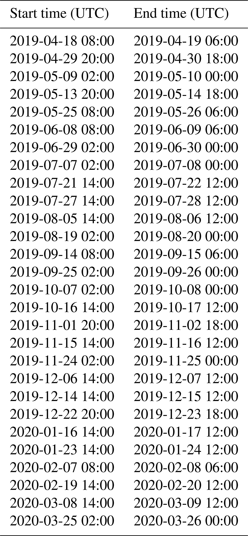
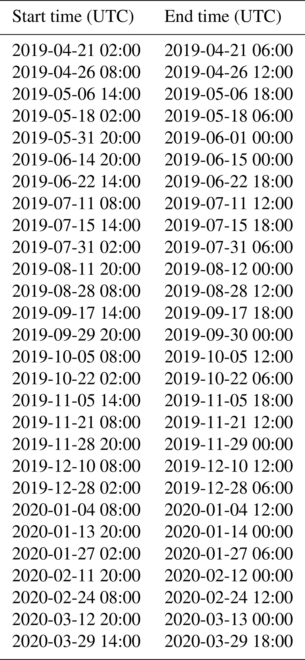
Table F3Time spans in the test set. All time spans were used in the evaluation of the single-frame and CoAtSaC algorithms. Only the time spans indicated in the third column were used in the evaluation of the tracking algorithm of Chevallier et al. (2023).
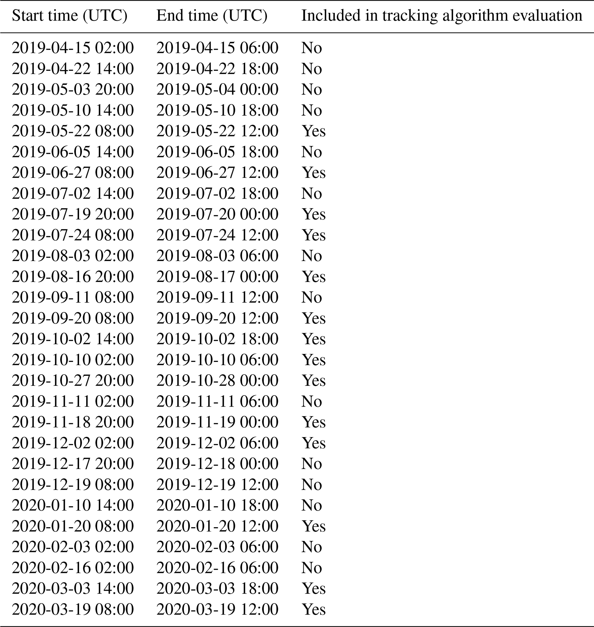
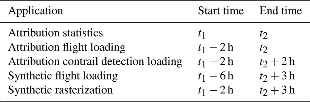
ERA5 data are available from the Copernicus Climate Change Service Climate Data Store (CDS): https://doi.org/10.24381/cds.bd0915c6 (Hersbach et al., 2023). Visualization of contrail detections on GOES-16 ABI data can be found at https://contrails.webapps.google.com/ (Google, 2025). Raw GOES-16 data can be found at https://console.cloud.google.com/storage/browser/gcp-public-data-goes-16 (NOAA, 2025). The SynthOpenContrails dataset described in this paper is available from the corresponding author upon request.
AS performed most of the design and implementation work for the CoAtSaC algorithm and the SynthOpenContrails dataset and also led the analysis and paper writing. VM contributed regular feedback on the approach and wrote parts of the paper. RC adapted the tracking algorithm to work on SynthOpenContrails, ran the SynthOpenContrails evaluations, and contributed to the paper writing. AD and KyM implemented the initial version of the synthetic contrail generation pipeline, upon which the SynthOpenContrails was built. SG helped design and implement the CoAtSaC algorithm and provided regular feedback on all aspects of the project. KeM helped design and implement the SynthOpenContrails dataset and provided regular feedback on all aspects of the project.
Some authors are employees of Google Inc., as noted in their author affiliations. Google is a technology company that sells computing services as part of its business.
Publisher’s note: Copernicus Publications remains neutral with regard to jurisdictional claims made in the text, published maps, institutional affiliations, or any other geographical representation in this paper. While Copernicus Publications makes every effort to include appropriate place names, the final responsibility lies with the authors.
We thank Tristan Abbott, Zebediah Engberg, and Marc Shapiro from Breakthrough Energy for their assistance with building and using the pycontrails library and for providing feedback on the overall approach and details along the way. We also thank Tharun Sankar, for his help with adapting pycontrails for our use; Sebastian Eastham, for his guidance throughout the project; and Dilip Krishnan, for the initial suggestion of applying RANSAC to this problem.
This paper was edited by Can Li and reviewed by two anonymous referees.
Agarwal, A., Meijer, V. R., Eastham, S. D., Speth, R. L., and Barrett, S. R. H.: Reanalysis-driven simulations may overestimate persistent contrail formation by 100 %–250 %, Environ. Res. Lett., 17, 014045, https://doi.org/10.1088/1748-9326/ac38d9, 2022. a, b, c, d
Akenine-Moller, T., Haines, E., and Hoffman, N.: Real-time rendering, AK Peters/crc Press, https://doi.org/10.1201/9781315365459, 2019. a
Akidau, T., Bradshaw, R., Chambers, C., Chernyak, S., Fernández-Moctezuma, R. J., Lax, R., McVeety, S., Mills, D., Perry, F., Schmidt, E., and Whittle, S.: The dataflow model: a practical approach to balancing correctness, latency, and cost in massive-scale, unbounded, out-of-order data processing, Proc. VLDB Endow., 8, 1792–1803, https://doi.org/10.14778/2824032.2824076, 2015. a
Apache Software Foundation: Apache Beam: An advanced unified programming model, https://beam.apache.org/documentation/programming-guide/ (last access: 6 September), 2024. a
Beer, A.: Bestimmung der Absorption des rothen Lichts in farbigen Flüssigkeiten, Ann. Phys., 162, 78–88, https://doi.org/10.1002/andp.18521620505, 1852. a, b
Bogacki, P. and Shampine, L.: A 3(2) pair of Runge – Kutta formulas, Appl. Math. Lett., 2, 321–325, https://doi.org/10.1016/0893-9659(89)90079-7, 1989. a
Borella, A., Boucher, O., Shine, K. P., Stettler, M., Tanaka, K., Teoh, R., and Bellouin, N.: The importance of an informed choice of CO2-equivalence metrics for contrail avoidance, Atmos. Chem. Phys., 24, 9401–9417, https://doi.org/10.5194/acp-24-9401-2024, 2024. a
Cameron, A. C., Gelbach, J. B., and Miller, D. L.: Bootstrap-Based Improvements for Inference with Clustered Errors, Rev. Econ. Stat., 90, 414–427, https://doi.org/10.1162/rest.90.3.414, 2008. a
Carver, R. W. and Merose, A.: ARCO-ERA5: An Analysis-Ready Cloud-Optimized Reanalysis Dataset, in: 103rd AMS Annual Meeting, AMS, 9 January 2023, Denver, CO, USA, 4A.1, https://ams.confex.com/ams/103ANNUAL/meetingapp.cgi/Paper/415842 (last access: 24 July 2025), 2023. a
Chevallier, R., Shapiro, M., Engberg, Z., Soler, M., and Delahaye, D.: Linear Contrails Detection, Tracking and Matching with Aircraft Using Geostationary Satellite and Air Traffic Data, Aerospace, 10, 578, https://doi.org/10.3390/aerospace10070578, 2023. a, b, c, d, e, f, g, h, i, j, k, l, m, n, o
Council of European Union: Commission Implementing Regulation (EU) 2024/2493 of 23 September 2024 amending Implementing Regulation (EU) 2018/2066 as regards updating the monitoring and reporting of greenhouse gas emissions pursuant to Directive 2003/87/EC of the European Parliament and of the Council, https://eur-lex.europa.eu/legal-content/EN/TXT/?uri=OJ:L_202402493 (last access: 17 July 2025), 2024. a
Driver, O. G. A., Stettler, M. E. J., and Gryspeerdt, E.: Factors limiting contrail detection in satellite imagery, Atmos. Meas. Tech., 18, 1115–1134, https://doi.org/10.5194/amt-18-1115-2025, 2025. a, b, c
DuBois, D. and Paynter, G. C.: ”Fuel Flow Method2” for Estimating Aircraft Emissions, SAE Transactions, 115, 1–14, https://doi.org/10.4271/2006-01-1987, 2006. a
Duda, D. P., Minnis, P., Nguyen, L., and Palikonda, R.: A Case Study of the Development of Contrail Clusters over the Great Lakes, J. Atmos. Sci., 61, 1132–1146, https://doi.org/10.1175/1520-0469(2004)061<1132:ACSOTD>2.0.CO;2, 2004. a
Garcia, M. A., Stafford, J., Minnix, J., and Dolan, J.: Aireon space based ADS-B performance model, in: 2015 Integrated Communication, Navigation and Surveillance Conference (ICNS), 21–23 April 2015, Herdon, VA, USA, C2-1–C2-10, https://doi.org/10.1109/ICNSURV.2015.7121219, 2015. a
Geraedts, S., Brand, E., Dean, T. R., Eastham, S., Elkin, C., Engberg, Z., Hager, U., Langmore, I., McCloskey, K., Yue-Hei Ng, J., Platt, J. C., Sankar, T., Sarna, A., Shapiro, M., and Goyal, N.: A scalable system to measure contrail formation on a per-flight basis, Environ. Res. Commun., 6, 015008, https://doi.org/10.1088/2515-7620/ad11ab, 2024. a, b, c, d, e, f, g, h, i, j, k, l, m, n, o, p, q, r, s, t, u, v, w, x, y, z, aa, ab, ac, ad
Gierens, K., Matthes, S., and Rohs, S.: How Well Can Persistent Contrails Be Predicted?, Aerospace, 7, 169, https://doi.org/10.3390/aerospace7120169, 2020. a, b, c
Golovin, D., Solnik, B., Moitra, S., Kochanski, G., Karro, J., and Sculley, D.: Google Vizier: A Service for Black-Box Optimization, in: Proceedings of the 23rd ACM SIGKDD International Conference on Knowledge Discovery and Data Mining, KDD '17, Association for Computing Machinery, New York, NY, USA, 1487–1495, ISBN 9781450348874, https://doi.org/10.1145/3097983.3098043, 2017. a
Goodman, S. J., Schmit, T. J., Daniels, J., and Redmon, R. J. (Eds.): The GOES-R series: a new generation of geostationary environmental satellites, Elsevier, ISBN 978-0-12-814327-8, 2020. a, b, c
Google: S2 Geometry, http://s2geometry.io/ (last access: 28 October 2024), 2024. a
Google: Contrails Explorer, https://contrails.webapps.google.com/ (last access: 17 July 2025), 2025. a
Gourgue, N., Boucher, O., and Barthès, L.: A dataset of annotated ground-based images for the development of contrail detection algorithms, Data in Brief, 59, 111364, https://doi.org/10.1016/j.dib.2025.111364, 2025. a
Gryspeerdt, E., Stettler, M. E. J., Teoh, R., Burkhardt, U., Delovski, T., Driver, O. G. A., and Painemal, D.: Operational differences lead to longer lifetimes of satellite detectable contrails from more fuel efficient aircraft, Environ. Res. Lett., 19, 084059, https://doi.org/10.1088/1748-9326/ad5b78, 2024. a, b, c
Hersbach, H., Bell, B., Berrisford, P., Hirahara, S., Horányi, A., Muñoz-Sabater, J., Nicolas, J., Peubey, C., Radu, R., Schepers, D., Simmons, A., Soci, C., Abdalla, S., Abellan, X., Balsamo, G., Bechtold, P., Biavati, G., Bidlot, J., Bonavita, M., De Chiara, G., Dahlgren, P., Dee, D., Diamantakis, M., Dragani, R., Flemming, J., Forbes, R., Fuentes, M., Geer, A., Haimberger, L., Healy, S., Hogan, R. J., Hólm, E., Janisková, M., Keeley, S., Laloyaux, P., Lopez, P., Lupu, C., Radnoti, G., de Rosnay, P., Rozum, I., Vamborg, F., Villaume, S., and Thépaut, J.-N.: The ERA5 global reanalysis, Q. J. Roy. Meteor. Soc., 146, 1999–2049, https://doi.org/10.1002/qj.3803, 2020. a, b, c
Hersbach, H., Bell, B., Berrisford, P., Biavati, G., Horányi, A., Muñoz Sabater, J., Nicolas, J., Peubey, C., Radu, R., Rozum, I., Schepers, D., Simmons, A., Soci, C., Dee, D., and Thépaut, J.-N.: ERA5 hourly data on pressure levels from 1940 to present, Copernicus Climate Change Service (C3S) Climate Data Store (CDS) [data set], https://doi.org/10.24381/cds.bd0915c6, 2023. a
Houchi, K., Stoffelen, A., Marseille, G. J., and De Kloe, J.: Comparison of wind and wind shear climatologies derived from high-resolution radiosondes and the ECMWF model, J. Geophys. Res.-Atmos., 115, D22123, https://doi.org/10.1029/2009JD013196, 2010. a
Jin, Z., Zhang, Y., Del Genio, A., Schmidt, G., and Kelley, M.: Cloud scattering impact on thermal radiative transfer and global longwave radiation, J. Quant. Spectrosc. Ra., 239, 106669, https://doi.org/10.1016/j.jqsrt.2019.106669, 2019. a
Kulik, L.: Satellite-based detection of contrails using deep learning, PhD thesis, Massachusetts Institute of Technology, https://hdl.handle.net/1721.1/124179, 2019. a
Lee, D., Fahey, D., Skowron, A., Allen, M., Burkhardt, U., Chen, Q., Doherty, S., Freeman, S., Forster, P., Fuglestvedt, J., Gettelman, A., De León, R., Lim, L., Lund, M., Millar, R., Owen, B., Penner, J., Pitari, G., Prather, M., Sausen, R., and Wilcox, L.: The contribution of global aviation to anthropogenic climate forcing for 2000 to 2018, Atmos. Environ., 244, 117834, https://doi.org/10.1016/j.atmosenv.2020.117834, 2021. a, b
Low, J., Teoh, R., Ponsonby, J., Gryspeerdt, E., Shapiro, M., and Stettler, M. E. J.: Ground-based contrail observations: comparisons with reanalysis weather data and contrail model simulations, Atmos. Meas. Tech., 18, 37–56, https://doi.org/10.5194/amt-18-37-2025, 2025. a
Mannstein, H., Meyer, R., and Wendling, P.: Operational detection of contrails from NOAA-AVHRR-data, Int. J. Remote Sens., 20, 1641–1660, https://doi.org/10.1080/014311699212650, 1999. a, b
Mannstein, H., Spichtinger, P., and Gierens, K.: A note on how to avoid contrail cirrus, Transport. Res. D-Tr. E., 10, 421–426, https://doi.org/10.1016/j.trd.2005.04.012, 2005. a
Mannstein, H., Brömser, A., and Bugliaro, L.: Ground-based observations for the validation of contrails and cirrus detection in satellite imagery, Atmos. Meas. Tech., 3, 655–669, https://doi.org/10.5194/amt-3-655-2010, 2010. a
Märkl, R. S., Voigt, C., Sauer, D., Dischl, R. K., Kaufmann, S., Harlaß, T., Hahn, V., Roiger, A., Weiß-Rehm, C., Burkhardt, U., Schumann, U., Marsing, A., Scheibe, M., Dörnbrack, A., Renard, C., Gauthier, M., Swann, P., Madden, P., Luff, D., Sallinen, R., Schripp, T., and Le Clercq, P.: Powering aircraft with 100 a
Martin Frias, A., Shapiro, M. L., Engberg, Z., Zopp, R., Soler, M., and Stettler, M. E. J.: Feasibility of contrail avoidance in a commercial flight planning system: an operational analysis, Environmental Research: Infrastructure and Sustainability, 4, 015013, https://doi.org/10.1088/2634-4505/ad310c, 2024. a, b
McCloskey, K., Geraedts, S., Jackman, B., Meijer, V. R., Brand, E., Fork, D., Platt, J. C., Elkin, C., and Van Arsdale, C.: A human-labeled Landsat-8 contrails dataset, in: Proceedings of the ICML 2021 Workshop on Tackling Climate Change with Machine Learning, virtually, 23 July 2020, vol. 23, 2021. a, b
Meerkötter, R., Schumann, U., Doelling, D., Minnis, P., Nakajima, T., and Tsushima, Y.: Radiative forcing by contrails, in: Annales Geophysicae, 17, 1080–1094, Springer, https://doi.org/10.1007/s00585-999-1080-7, 1999. a
Meijer, V. R.: Satellite-based Analysis and Forecast Evaluation of Aviation Contrails, PhD thesis, Massachusetts Institute of Technology, https://hdl.handle.net/1721.1/155350, 2024. a, b, c
Meijer, V. R., Kulik, L., Eastham, S. D., Allroggen, F., Speth, R. L., Karaman, S., and Barrett, S. R. H.: Contrail coverage over the United States before and during the COVID-19 pandemic, Environ. Res. Lett., 17, 034039, https://doi.org/10.1088/1748-9326/ac26f0, 2022. a, b
Meijer, V. R., Eastham, S. D., Waitz, I. A., and Barrett, S. R. H.: Contrail altitude estimation using GOES-16 ABI data and deep learning, Atmos. Meas. Tech., 17, 6145–6162, https://doi.org/10.5194/amt-17-6145-2024, 2024. a, b, c
Minnis, P., Young, D. F., Garber, D. P., Nguyen, L., Smith Jr., W. L., and Palikonda, R.: Transformation of contrails into cirrus during SUCCESS, Geophys. Res. Lett., 25, 1157–1160, https://doi.org/10.1029/97GL03314, 1998. a
Ng, J. Y.-H., McCloskey, K., Cui, J., Meijer, V. R., Brand, E., Sarna, A., Goyal, N., Van Arsdale, C., and Geraedts, S.: Contrail Detection on GOES-16 ABI With the OpenContrails Dataset, IEEE T. Geosci. Remote, 62, 1–14, https://doi.org/10.1109/TGRS.2023.3345226, 2024. a, b, c, d, e, f, g, h, i, j, k, l, m, n, o, p, q, r, s, t, u, v, w
National Oceanic and Atmospheric Administration (NOAA): GOES-16 Geostationary Operational Environmental Satellite data, NOAA [data set], https://console.cloud.google.com/storage/browser/gcp-public-data-goes-16, last access: 24 July 2025. a
Okuyama, A., Andou, A., Date, K., Hoasaka, K., Mori, N., Murata, H., Tabata, T., Takahashi, M., Yoshino, R., and Bessho, K.: Preliminary validation of Himawari-8/AHI navigation and calibration, in: Earth Observing Systems XX, edited by: Butler, J. J., Xiong, X. J., and Gu, X., International Society for Optics and Photonics, SPIE, 9607, 96072E, https://doi.org/10.1117/12.2188978, 2015. a
Petzold, A., Thouret, V., Gerbig, C., Zahn, A., Brenninkmeijer, C. A. M., Gallagher, M., Hermann, M., Pontaud, M., Ziereis, H., Boulanger, D., Marshall, J., Nédélec, P., Smit, H. G. J., Friess, U., Flaud, J.-M., Wahner, A., Cammas, J.-P., Volz-Thomas, A., and IAGOS Team: Global-scale atmosphere monitoring by in-service aircraft – current achievements and future prospects of the European Research Infrastructure IAGOS, Tellus B, 67, 28452, https://doi.org/10.3402/tellusb.v67.28452, 2015. a
Poll, D. and Schumann, U.: An estimation method for the fuel burn and other performance characteristics of civil transport aircraft in the cruise. Part 1 fundamental quantities and governing relations for a general atmosphere, Aeronaut. J., 125, 257–295, https://doi.org/10.1017/aer.2020.62, 2021. a
Price, I., Sanchez-Gonzalez, A., Alet, F., Andersson, T. R., El-Kadi, A., Masters, D., Ewalds, T., Stott, J., Mohamed, S., Battaglia, P., Lam, R., and Willson, M.: Probabilistic weather forecasting with machine learning, Nature, 637, 84–90, https://doi.org/10.1038/s41586-024-08252-9, 2025. a
Sausen, R., Hofer, S., Gierens, K., Bugliaro, L., Ehrmanntraut, R., Sitova, I., Walczak, K., Burridge-Diesing, A., Bowman, M., and Miller, N.: Can we successfully avoid persistent contrails by small altitude adjustments of flights in the real world?, Meteorol. Z., 33, 83–98, https://doi.org/10.1127/metz/2023/1157, 2024. a, b, c, d
Schumann, U.: On conditions for contrail formation from aircraft exhausts, Meteorol. Z., 5, 4–23, https://doi.org/10.1127/metz/5/1996/4, 1996. a
Schumann, U.: A contrail cirrus prediction model, Geosci. Model Dev., 5, 543–580, https://doi.org/10.5194/gmd-5-543-2012, 2012. a, b, c, d, e, f, g, h, i, j, k, l, m
Schumann, U., Mayer, B., Graf, K., and Mannstein, H.: A Parametric Radiative Forcing Model for Contrail Cirrus, J. Appl. Meteorol. Clim., 51, 1391–1406, https://doi.org/10.1175/JAMC-D-11-0242.1, 2012. a
Schumann, U., Hempel, R., Flentje, H., Garhammer, M., Graf, K., Kox, S., Lösslein, H., and Mayer, B.: Contrail study with ground-based cameras, Atmos. Meas. Tech., 6, 3597–3612, https://doi.org/10.5194/amt-6-3597-2013, 2013. a
Schumann, U., Penner, J. E., Chen, Y., Zhou, C., and Graf, K.: Dehydration effects from contrails in a coupled contrail–climate model, Atmos. Chem. Phys., 15, 11179–11199, https://doi.org/10.5194/acp-15-11179-2015, 2015. a
Shapiro, M., Engberg, Z., Teoh, R., Stettler, M., Dean, T., and Abbott, T.: pycontrails: Python library for modeling aviation climate impacts, Zenodo, https://doi.org/10.5281/zenodo.13357046, 2024. a, b
Sonabend, A., Elkin, C., Dean, T., Dudley, J., Ali, N., Blickstein, J., Brand, E., Broshears, B., Chen, S., Engberg, Z., et al.: Feasibility test of per-flight contrail avoidance in commercial aviation, Commun. Eng., 3, 184, https://doi.org/10.1038/s44172-024-00329-7, 2024. a, b, c, d, e, f, g, h
Teoh, R., Schumann, U., Majumdar, A., and Stettler, M. E. J.: Mitigating the Climate Forcing of Aircraft Contrails by Small-Scale Diversions and Technology Adoption, Environ. Sci. Technol., 54, 2941–2950, https://doi.org/10.1021/acs.est.9b05608, 2020. a, b
Torr, P. H.: Geometric motion segmentation and model selection, Philos. T. Roy. Soc. A, 356, 1321–1340, https://doi.org/10.1098/rsta.1998.0224, 1998. a
Vazquez-Navarro, M., Mannstein, H., and Mayer, B.: An automatic contrail tracking algorithm, Atmos. Meas. Tech., 3, 1089–1101, https://doi.org/10.5194/amt-3-1089-2010, 2010. a
Vázquez-Navarro, M., Mannstein, H., and Kox, S.: Contrail life cycle and properties from 1 year of MSG/SEVIRI rapid-scan images, Atmos. Chem. Phys., 15, 8739–8749, https://doi.org/10.5194/acp-15-8739-2015, 2015. a
Voigt, C., Kleine, J., Sauer, D., Moore, R. H., Bräuer, T., Le Clercq, P., Kaufmann, S., Scheibe, M., Jurkat-Witschas, T., Aigner, M., Bauder, U., Boose, Y., Borrmann, S., Crosbie, E., Diskin, G. S., DiGangi, J., Hahn, V., Heckl, C., Huber, F., Nowak, J. B., Rapp, M., Rauch, B., Robinson, C., Schripp, T., Shook, M., Winstead, E., Ziemba, L., Schlager, H., and Anderson, B. E.: Cleaner burning aviation fuels can reduce contrail cloudiness, Commun. Earth Environ., 2, 114, https://doi.org/10.1038/s43247-021-00174-y, 2021. a
Zhang, C., Chen, L., Ding, S., Zhou, X., Chen, R., Zhang, X., Yu, Z., and Wang, J.: Mitigation effects of alternative aviation fuels on non-volatile particulate matter emissions from aircraft gas turbine engines: A review, Sci. Total Environ., 820, 153233, https://doi.org/10.1016/j.scitotenv.2022.153233, 2022. a
- Abstract
- Introduction
- Synthetic contrail benchmark dataset
- Contrail-to-flight attribution algorithm
- Results
- Conclusions
- Appendix A: Synthetic dataset generation
- Appendix B: Synthetic dataset design decisions
- Appendix C: Attribution algorithm design decisions
- Appendix D: Modifications to previously published attribution algorithms
- Appendix E: Performance as a function of contrail properties
- Appendix F: Time spans and dataset splits
- Data availability
- Author contributions
- Competing interests
- Disclaimer
- Acknowledgements
- Review statement
- References