Improving consistency in methane emission quantification from the natural gas distribution systems across measurement devices

Mobile real-time measurements of ambient methane provide a fast and effective method to identify and quantify methane leaks from local gas distribution systems in urban areas. The objectives of these methodologies are to (i) identify leak locations for repair and (ii) construct measurement-based emission rate estimates, which can improve emissions reporting and contribute to monitoring emission changes over time. Currently, the most common method for emission quantification uses the maximum methane enhancement detected while crossing a methane plume. However, the recorded maximum depends on instrument characteristics, such as measurement cell size, pump speed, and measurement frequency. Consequently, the current approach can only be used by instruments with similar characteristics. We suggest that the integrated spatial peak area is a more suitable quantity that can eliminate the bias between different instruments. Based on controlled release experiments conducted with various devices in four cities (London, Toronto, Rotterdam, and Utrecht), emission estimation methodologies were evaluated. Indeed, when different analysers were measuring in the same vehicle and from the same air inlet, the integrated spatial peak area was found to be a more robust metric across different methane gas analyser devices than the maximum methane enhancement. A statistical function based on integrated spatial peak area is proposed for more consistent emission estimations when using different instruments. On top of this systematic relation between actual emission rate and recorded spatial peak area, large variations in methane spatial peak area were observed for the multiple transects across the same release point, in line with previous experiments. This variability is the main contributor to uncertainty in efforts to use mobile measurements to prioritize leak repair. We show that repeated transects can reduce this uncertainty and improve the categorization into different leak categories. We recommend a minimum of three and an optimal range of five–seven plume transects for effective emission quantification to prioritize repair actions.

1 Introduction

Mitigating methane (CH₄) emissions is an important step to combat climate change. The increase in atmospheric CH₄ has contributed approximately 30 % of global warming since pre-industrial times (IPCC, 2023). CH₄ has an 82 times higher global warming potential over 20 years (Forster et al., 2021) and a shorter atmospheric lifetime (9.1 ± 0.9 years; Szopa et al., 2021) than CO₂. This offers the opportunity for reductions in climate warming by reducing CH₄ emissions, possibly avoiding temperature overshoots (Hu et al., 2013; Collins et al., 2018). General awareness of the importance for timely CH₄ mitigation is rising. More than 150 nations have joined the Global Methane Pledge, established during the UN Climate Change Conference of the Parties (COP 26) in 2021, pledging to reduce human-made CH₄ emissions in 2030 by 30 % relative to 2020 (EU Commission, 2021). Following this, regulations specifically targeting CH₄ emissions have been adopted or are underway, for example, in Canada, Colombia, the EU, and the U.S. (Environment and Climate Change Canada, 2022; Ministerio de Minas y Energía, 2022; EU Commission, 2023; U.S. Environmental Protection Agency, 2023).

About a quarter of total global anthropogenic CH₄ emissions can be attributed to the oil and natural gas sector (Saunois et al., 2020). The International Energy Agency (2023) suggests that deploying existing technological solutions could cut 75 % of global oil and gas CH₄ emissions, at a cost less than 3 % of the net income of the oil and gas industry in 2022. After the production segment, emission intensity is highest in the downstream distribution segment (Cooper et al., 2021; International Energy Agency, 2023). Regionally, this sector can even represent the largest share, especially in the EU, where the vast majority of oil and gas used is imported (EU Commission, 2023).

Leak detection, quantification, and verification surveys are key to mitigating CH₄ emissions from the oil and gas supply chain. CH₄ analysers on various platforms such as satellites, aircraft, or vehicles have been utilized to detect and quantify fossil-fuel-related CH₄ emissions (Jacob et al., 2016; Cui et al., 2019; Maazallahi et al., 2020; Irakulis-Loitxate et al., 2021; Shen et al., 2021; Zavala-Araiza et al., 2021; Korbeń et al., 2022). Both rapid detection and reliable quantification can help to improve and prioritize capital-intensive leak repair efforts (von Fischer et al., 2017). This is especially important since leak distributions have been found to be skewed, a few large leaks being responsible for a major share of total emissions (Zavala-Araiza et al., 2015; Omara et al., 2016; Robertson et al., 2017; Maazallahi et al., 2020; Weller et al., 2020; Stavropoulou et al., 2023). Beyond the direct mitigation opportunity, reliable quantification can help to evaluate the scale of fugitive emissions and possible emission reductions over time, related to the Global Methane Pledge. Vehicle-based mobile measurements deploying fast CH₄ gas analysers have proven to be an efficient method for quickly and effectively surveying distribution networks across urban areas. There is currently no universally accepted measurement and data analysis methodology in place. Most widely used is the statistical methodology developed by von Fischer et al. (2017) and later refined by Weller et al. (2019). Based on controlled release experiment data (von Fischer et al., 2017), they derived the following relation between the observed maximum excess CH₄ (in ppm) when crossing a plume and the release rate (r_E, in L min⁻¹):

$$\begin{array}{}\text{(1)}& \ln \left({\left[{\mathrm{CH}}_{\mathrm{4}}\right]}_{max}\right)=\mathrm{0.817}\cdot \ln \left(r_{\mathrm{E}}\right)-\mathrm{0.988}.\end{array}$$

In the original multivariate regression model suggested by von Fischer et al. (2017), the release rate was used as the response variable, and maximum enhancement, integrated spatial peak area, and an index of the plume kurtosis were used as predictors. Weller et al. (2019) argued that maximum CH₄ enhancement proved to be the best predictor of the release rate and that additional predictors did not meaningfully improve emission rate estimates.

This transfer equation has been applied in several measurement campaigns in North America and Europe (Phillips et al., 2013; von Fischer et al., 2017; Weller et al., 2018; Ars et al., 2020; Maazallahi et al., 2020; Defratyka et al., 2021; Fernandez et al., 2022; Wietzel and Schmidt, 2023; Vogel et al., 2024). During each survey, hundreds to thousands of leak indications were detected. The emission estimates were also used to rank leak indications into different categories (high is > 40 L min⁻¹, medium is 6–40 L min⁻¹, and small is < 6 L min⁻¹ emissions) to assist with repair prioritization decisions (von Fischer et al., 2017; Maazallahi et al., 2020). However, several problems have been identified. Leak indications cannot always be confirmed through re-measurement, and gas providers cannot always determine the source of the emissions (von Fischer et al., 2017; Weller et al., 2018; Maazallahi et al., 2020). Furthermore, environmental factors, such as wind but also dispersion and turbulence within the emission plume, lead to large uncertainties in measurements with corresponding over- and underestimations. Especially within urban built environments, complex wind flow, re-circulation, and dispersion patterns play an important role (Carpentieri and Robins, 2015; Raz̆njević, 2023). In addition, the approach developed in von Fischer et al. (2017) was derived for measurements using one specific device (Picarro G2301). By now, multiple CH₄ analysers are in use, and it has been shown that CH₄ enhancements measured with different instruments can differ substantially (Gillespie et al., 2023; Maazallahi et al., 2023). These discrepancies are expected, as different analysers exhibit distinct instrument characteristics. Parameters such as cell volume, cell temperature, cell pressure, measurement frequency, and flow rate vary among instruments, all of which influence the detected shape of the CH₄ peak (Takriti et al., 2021). Thus, the transfer function developed by Weller et al. (2019), where estimated emission rates purely depend on the measured peak maximum, is not transferable to other analysers.

Maazallahi et al. (2020) noted that the integrated spatial peak area is much more consistent than the peak maximum between two different instruments operated in parallel during mobile measurement campaigns in Hamburg and Utrecht. Gillespie et al. (2023) conducted controlled release experiments and street-level measurements in Toronto, using two CH₄ devices. By applying Gaussian plume inversions to both CH₄ peak maximum and peak area, they concluded that emission rates should be estimated using either the peak area or, if relying on enhancement height, incorporating explicit modelling of the instrument response function to account for variations in cell residence time. Ars et al. (2020) found the maximum amplitude of CH₄ enhancement to be 50 %–80 % lower when sampled with a high inlet at 2.5 m compared to sampling close to the ground, whereas the integrated spatial peak area was better comparable between the measurements at different heights.

This study evaluates results from different controlled CH₄ release experiments in four cities and evaluates predictors for statistical emission rate estimation. Specifically, we evaluate the consistency between measured peak heights and spatial peak areas across eight different instruments when transecting the same emission plume with the same air inlet. We then propose an instrument-independent transfer equation that uses the integrated spatial peak area. We evaluate how successful this transfer equation is in categorizing emissions for single and multiple passes.

2 Methods

In this section, we first describe the controlled release experiments conducted to generate the dataset (Sect. 2.1). We then outline the data processing steps, including peak identification and calculation of the spatial peak area (Sect. 2.2). Next, we present the approach for estimating emission rates from the measurements (Sect. 2.3). Finally, we evaluate the performance of the quantification method (Sect. 2.4), considering both its categorization ability and the impact of the number of transects on estimation accuracy.

2.1 Controlled release experiments

Controlled release experiments (CREs) were conducted with a total of nine different analysers in four different cities (London, Rotterdam, Toronto, and Utrecht) situated in three different countries and conducted by different research groups (Table 1). The release locations are visualized in the Supplement, Fig. S1, and an overview of the specific release rates per release location is given in the Supplement, Table S2.

Table 1 Controlled release experiments: overview of cities, release rates, inlet height, and location. In all experiments, the release height was set at ground level.

^a Picarro INC, Santa Clara, USA. ^b Los Gatos Research, San Jose, USA. ^c LI-COR Environmental, Lincoln, USA. ^d Aerodyne Research, Billerica, USA. ^e Aeris Technologies, Eden Landing Road, Hayward, CA. ^f MIRO Analytical AG, Wallisellen, CH.

The controlled release experiment in Rotterdam was conducted on 6 September 2022 (Maazallahi et al., 2025a). The location was selected to reflect common urban characteristics with houses, parked cars, and overhanging trees (see Fig. S2). Methane (purity > 99.9 %) was released through a $\mathrm{1}/\mathrm{4}$ in. O.D. Teflon tube from two cylinders placed at a total of three locations along two connected streets at a wide range of flow rates (0.15–120 L min⁻¹). However, at two of the three locations, the rotameter used to adjust the release rate was suspected to not work properly. Therefore, only releases at location 1 (flow rate controlled electronically by an Alicat MCP-100SLPM, 5–120 L min⁻¹) are considered. The release occurred 1–3 m from the street, with the inlet line moved to 5 m for flow rates above 40 L min⁻¹. Atmospheric CH₄ mole fraction was measured while driving along the release locations using five different instruments distributed over two vehicles. The first vehicle is Utrecht University's Air Quality car (UUAQ, Institute for Risk Assessment Sciences, Utrecht University), an Opel Astra with an air inlet on its roof (inlet height ca. 1.7 m, see Fig. S2). This car contained two cavity ring-down spectroscopy (CRDS) analysers, models G2301 and G4302, and a mid-infrared laser absorption spectroscopy analyser MIRA Ultra. Two instruments, a MGA10 analyser and a TILDAS dual laser trace gas analyser, were utilized in the measurement trailer of a semi-trailer truck operated by the Netherlands Organisation for Applied Scientific Research (TNO). The inlet is on the side of the trailer, around 2.5 m above ground level. In the morning, both vehicles drove separately. During the afternoon session, the G4302 and MIRA Ultra analysers were transferred to the TNO truck to facilitate better comparison between the measuring devices, and the UUAQ vehicle ceased its mobile measurements.

Two experiments in Utrecht were conducted at the Utrecht Science Park with multi-storey office and service buildings to the sides of the street (see Fig. S3; Maazallahi et al., 2025b; Tettenborn et al., 2025b). On 25 November 2022, CH₄ was released simultaneously at two different locations. Two manual flowmeters (Krohne DK800/PV (25–250 NL h⁻¹) at location 1 and Krohne DK800/PV (500–5000 NL h⁻¹) at location 2) were used to measure the release rates (spanning from 2.18–15 L min⁻¹), which were controlled by the pressure reducer of the cylinder. CH₄ mole fractions were measured by the G2301 and G4302 devices, the same devices used during the Rotterdam campaign, on board the UUAQ car. The car was driving in a circle around two buildings, passing each emission point once per circle. On 11 June 2024, CH₄ was released simultaneously at the same site (0.15–100 L min⁻¹) and measured by the G2301 and MIRA Ultra instruments installed in the van of the Institute for Marine and Atmospheric Research Utrecht (Maazallahi et al., 2020). Initially, the two release locations from the previous experiment were used. Due to power issues at location 1, the release point was moved across the street soon after the start. An Alicat device (high rates) and an MKS (PR 4000) controller (low rates) were used. Initially, the Alicat was at location 1 and the MKS was at location 2. Midway, they were switched to enable all release rates at both sites.

Nearby London (on an open airfield near Bedford), two measurement campaigns were carried out, the first on 10–13 September 2019 (35 and 70 L min⁻¹; France et al., 2025a) and the second on 13 and 14 May 2024 (0.2–70.5 L min⁻¹; France et al., 2025b). A G2301 analyser was used on all days in the first campaign; on 10 September, additionally, an ultraportable methane: ethane analyser and on 11 September, a LI-7810 ${\mathrm{CH}}_{\mathrm{4}}/{\mathrm{CO}}_{\mathrm{2}}/{\mathrm{H}}_{\mathrm{2}}\mathrm{O}$ trace gas analyser were used. For the second campaign, only data collected by the LI-7810 instrument were evaluated for this study. The driving pattern consisted of parallel legs perpendicular to the estimated wind direction, gradually moving away from the source.

In Toronto, two CREs were carried out (Gillespie et al., 2025). In the Toronto industrial Port Lands neighbourhood, both a mobile bicycle-trailer-based laboratory equipped with a UGGA analyser (inlet at 1.6 m above ground) and a vehicle-based setup measuring with a G2401 analyser (inlet at 2.5 m above the ground) were deployed on 20 October 2021 (2.5–20 L min⁻¹). The second experiment was carried out on 24 October 2021 on a parking lot, deploying the same vehicle-based setup (0.1–5 L min⁻¹).

The average driving speed during plume transects was 3.8 ± 1.0, 5.6 ± 0.9, 5.9 ± 0.9, 3.0 ± 0.5 to 3.9 ± 0.4, 6.0 ± 1.5 to 7.3 ± 1.4, and 4.0 ± 0.4 to 7.5 ± 0.9 m s⁻¹ in Rotterdam, Utrecht I, Utrecht II, London I, London II, and Toronto, respectively. The median distance between the location where the plumes were detected and the release location was 20, 20, 21, 20 to 25, 21 to 22, and 17 to 24 m, which is typical for urban gas distribution networks (see Supplement, Sect. S6). More detailed descriptions of the measurement devices, experimental setup, and the CH₄ time series can be found in the Supplement (Sect. S1–S4) and are supported by Maazallahi et al. (2020), Gillespie et al. (2023), and Vogel et al. (2024).

2.2 Data treatment, peak identification, determining peak maximum, and spatial peak area

The raw measurements were calibrated and corrected for inlet delay and a delay between different instruments (see Sect. S3). A centred 5 min moving window was applied to determine the atmospheric CH₄ background level at each point in time. The background level was defined as the 10th percentile of the CH₄ mole fraction measurements, which was assessed to represent the background well (comparison is given in Sect. S5). A peak was identified as a CH₄ enhancement reaching above 102 % of the background level. CH₄ enhancements in the calibrated CH₄ dataset were detected utilizing the Python scipy function find_peaks (Virtanen et al., 2020). Those individual peaks were then manually quality checked for overlap of peaks, flawless function of all instruments deployed, validity of the transect, and car speed. When multiple instruments recorded measurements in one vehicle, the peak finding algorithm was applied to only one of the instruments. With a manual quality check, it was ensured that the peak was valid for all instruments. For the London datasets, peaks obtained at a distance further than 75 m from the source were omitted to keep the distance within the same limits as for the other CREs. The maximum CH₄ enhancement within the time interval of each peak was determined for each instrument. The peak finder algorithm was applied to the G4302 device for the measurements on the UUAQ car in Rotterdam; in Utrecht I, the G2301 instrument; for Utrecht II, the MGA10 device for the measurement on the TNO truck in Rotterdam; and the uMEA and G2301-m device during the CREs in London I for Day 1 and Day 2, respectively. The peak area was integrated over space rather than time to take different driving speeds into account. To convert the time series to the spatial coordinate, the CH₄ mole fraction enhancement at time t_i+1 (c(t_i+1), parts per million) after subtraction of the CH₄ background level) was multiplied by the measurement time step of the individual instrument (Δt = $t_{i+\mathrm{1}}-t_i$) and the velocity of the vehicle averaged over the whole peak duration (${\stackrel{\mathrm{‾}}{v}}_{\mathrm{peak}}$), yielding the integrated spatial peak area $\left({\left[{\mathrm{CH}}_{\mathrm{4}}\right]}_{\mathrm{area}}\right)$ in ppm ⋅ m.

$$\begin{array}{}\text{(2)}& {\left[{\mathrm{CH}}_{\mathrm{4}}\right]}_{\mathrm{area}}=\sum _{i=\mathrm{0}}^n\mathrm{\Delta }t\cdot c\left(t_{i+\mathrm{1}}\right)\cdot {\stackrel{\mathrm{‾}}{v}}_{\mathrm{peak}}.\end{array}$$

It is important to note that this spatial peak area does not correspond to the integration of CH₄ enhancement of the physical CH₄ plume in the environment across a 2D plane in space. Rather, it represents a linear 1D fraction of the plume that is described by the driving track.

2.3 Emission rate estimation

An ordinary least-squares regression model (scipy.stats.linregress library, Virtanen et al., 2020) was applied to the spatial peak areas of the combined dataset. The natural logarithm (ln) of the known release rate was used as the independent variable, and the ln of integrated spatial peak area of CH₄ enhancements was used as the dependent variable, calculated as follows:

$$\begin{array}{}\text{(3)}& \ln \left({\left[{\mathrm{CH}}_{\mathrm{4}}\right]}_{\mathrm{area}}\right)=a_{\mathrm{1}}\ln \left(r_{\mathrm{E}}\right)+a_{\mathrm{0}}.\end{array}$$

The fitting was performed using the entire dataset, without separating it into training and testing data. To assess the conformity of the data with the assumptions underlying linear regression (normality, linearity, independence, and homoscedasticity), several analyses were carried out (Sect. S7). A similar fit was applied to the maximum excess CH₄ ($\ln \left({\left[{\mathrm{CH}}_{\mathrm{4}}\right]}_{max}\right)=a_{\mathrm{1}}^{max}\ln \left(r_{\mathrm{E}}\right)+a_{\mathrm{0}}^{max}$), for comparison with the equation from Weller et al. (2019).

To infer emission rate estimations based on measurements, the linear regression needs to be solved for the release rate. Then the equation can be applied to measurements: the Weller equation to the peak maximum measurements and the area equation to the corresponding area measurements, for both cases with background levels subtracted from CH₄ measurements. Sometimes, the algorithm produces estimates far outside the calibration range of the method; therefore, a cap of 200 L min⁻¹ was imposed on emission rate estimations for the following evaluation.

2.4 Evaluating quantification performance

2.4.1 Categorization

For each valid plume transect (i) in the dataset used to derive the regression model, emission rates were estimated utilizing both estimation methods, applying the inverse of Eqs. (1) and (3).

$$\begin{array}{}\text{(4)}& {\displaystyle }\begin{array}{rl}& {\left(r_{\mathrm{E},\mathrm{Weller}\mathrm{equation}}\right)}_i=\exp \left({\displaystyle \frac{\mathrm{1}}{a_{\mathrm{1}}^{\mathrm{W}}}}\left(\ln {\left({\left[{\mathrm{CH}}_{\mathrm{4}}\right]}_{max}\right)}_i-a_{\mathrm{0}}^{\mathrm{W}}\right)\right)\\ & =\exp \left({\displaystyle \frac{\mathrm{1}}{\mathrm{0.817}}}\left(\ln {\left({\left[{\mathrm{CH}}_{\mathrm{4}}\right]}_{max}\right)}_i+\mathrm{0.988}\right)\right),\end{array}\text{(5)}& {\displaystyle }{\left(r_{\mathrm{E},\mathrm{area}\mathrm{equation}}\right)}_i=\exp \left({\displaystyle \frac{\mathrm{1}}{a_{\mathrm{1}}^{\mathrm{A}}}}\left(\ln {\left({\left[{\mathrm{CH}}_{\mathrm{4}}\right]}_{\mathrm{area}}\right)}_i-a_{\mathrm{0}}^{\mathrm{A}}\right)\right).\end{array}$$

The superscripts W (Weller equation) and A (area equation) differentiate the regression parameters. Subsequently, an estimated category was assigned to each peak given these inferred emission rates. To remain consistent with previous studies, release rates were classified into four different categories (< 0.5 L min⁻¹ – very low, 0.5–6 L min⁻¹ – low, 6–40 L min⁻¹ – medium, and > 40 L min⁻¹ – high). This approach follows von Fischer et al. (2017) but is extended by a category for very small emissions as used in Vogel et al. (2024). For each group of peaks belonging to the same category, the percentage of correctly classified peaks was calculated, along with the percentages of peaks that were erroneously categorized into other categories.

2.4.2 Percentage difference in emission estimation as a function of the number of transects

As will be shown below, variability in the plume shape causes large differences in observed peak maxima, spatial peak areas, and thus derived emission rates for individual transects at the same actual emission rate. This variability can be reduced by evaluating the average of several transects at the same emission rate. Following the analysis in Luetschwager et al. (2021), the effect of the number of detections per CH₄ source on variability in estimated emission rate was explored.

Two approaches were followed to evaluate the emission quantification:

1. Comparison against the mean emission rate calculated from the leak indications (following Luetschwager et al., 2021).

2. Comparison against the true release rate, which is known for our experiments.

To calculate the mean emission rates for the former comparison, the average natural logarithm of the integrated spatial peak area across all observed instances associated with each release rate j was computed as

$$\begin{array}{}\text{(6)}& {\stackrel{\mathrm{‾}}{\ln \left({\left[{\mathrm{CH}}_{\mathrm{4}}\right]}_{\mathrm{area}}\right)}}_j={\displaystyle \frac{\mathrm{1}}{n}}\sum _{i=\mathrm{1}}^n\ln {\left({\left[{\mathrm{CH}}_{\mathrm{4}}\right]}_{\mathrm{area}}\right)}_{i,j}.\end{array}$$

For each release rate, one mean emission rate estimation (r_E,mean)_j was obtained by applying the area equation to the calculated ${\stackrel{\mathrm{‾}}{\ln \left({\left[{\mathrm{CH}}_{\mathrm{4}}\right]}_{\mathrm{area}}\right)}}_j$. Subsequently, a Monte Carlo simulation was performed, where we randomly selected between 2–10 emission peaks i at each release rate and averaged the natural logarithm of the integrated spatial peak areas. Measurements obtained by different instruments during the same transects were treated as separate peaks. The theoretical number of possible subsets N from a certain size of set M with replacement is $\left(\begin{array}{c}M+N-\mathrm{1}\\ N\end{array}\right)=\frac{\left(M+N-\mathrm{1}\right)\mathrm{!}}{N\mathrm{!}\cdot \left(M-\mathrm{1}\right)\mathrm{!}}$. This gives, for example, between 465 and 6×10⁷ combinations for N between 2–10 and M = 30. This procedure was repeated 2000 times for each release rate and number of detections. That means for N = 3, 3 peaks were randomly sampled 2000 times from a given release rate, yielding 2000 emission rate estimations ${\left(r_{\mathrm{E},\mathrm{sim}}\right)}_{k,j,N}$ ($k\in \left[\mathrm{1},\mathrm{2000}\right]$) for each release rate. For each of those 2000 emission rate estimations as ${\left(r_{\mathrm{E},\mathrm{sim}}\right)}_{k,j,N}$, the percentage difference to the mean emission rate estimation ${\left(r_{\mathrm{E},\mathrm{mean}}\right)}_j$ and the known release rate ${\left(r_{\mathrm{E},\mathrm{true}}\right)}_j$ were calculated as

$$\begin{array}{}\text{(7)}& {\displaystyle }{\left(\mathrm{\Delta }{\mathit{\%}}_{\mathrm{mean}}\right)}_{k,j,N}={\displaystyle \frac{{\left(r_{\mathrm{E},\mathrm{sim}}\right)}_{k,j,N}-{\left(r_{\mathrm{E},\mathrm{mean}}\right)}_j}{{\left(r_{\mathrm{E},\mathrm{mean}}\right)}_j}}\cdot \mathrm{100}\mathit{\%},\text{(8)}& {\displaystyle }{\left(\mathrm{\Delta }{\mathit{\%}}_{\mathrm{true}}\right)}_{k,j,N}={\displaystyle \frac{{\left(r_{\mathrm{E},\mathrm{sim}}\right)}_{k,j,N}-{\left(r_{\mathrm{E},\mathrm{true}}\right)}_j}{{\left(r_{\mathrm{E},\mathrm{true}}\right)}_j}}\cdot \mathrm{100}\mathit{\%}.\end{array}$$

Then, an average percentage deviation for each release rate j and number of transects N was determined for both cases as

$$\begin{array}{}\text{(9)}& {\left(\stackrel{\mathrm{‾}}{\mathrm{\Delta }\mathit{\%}}\right)}_{j,N}={\displaystyle \frac{\mathrm{1}}{\mathrm{2000}}}\sum _{k=\mathrm{1}}^{\mathrm{2000}}{\left(\mathrm{\Delta }\mathit{\%}\right)}_{k,j,N}.\end{array}$$

Finally, an average over the different release rates J for each number of transects $N\in \left[\mathrm{2},\mathrm{10}\right]$ was calculated for both cases:

$$\begin{array}{}\text{(10)}& {〈\stackrel{\mathrm{‾}}{\mathrm{\Delta }\mathit{\%}}〉}_N={\displaystyle \frac{\mathrm{1}}{J}}\sum _{j=\mathrm{1}}^J{\left(\stackrel{\mathrm{‾}}{\mathrm{\Delta }\mathit{\%}}\right)}_{j,N}.\end{array}$$

The analysis was done for each unique release rate and location pair. Experiments with fewer than 10 transects were filtered out, as the Monte Carlo analysis samples up to 10 measurements (N ranging from 2 to 10) from the available transects. This leaves 35 of the original 55 release rates. Lastly, another categorization analysis was conducted with the goal to investigate the classification performance when incorporating multiple transects. For each of the 2000 mean emission rates per release rate and number of transects, a category was assigned and evaluated.

3 Results and discussion

In this section, we present and analyse the key findings of our study. First, we evaluate instrument performance by comparing peak maximum and spatial peak area as metrics for emission quantification (Sect. 3.1). Next, we introduce a method for converting spatial peak areas into emission rate estimates (Sect. 3.2). We then explore how survey data can be used to support repair prioritization (Sect. 3.3). Additionally, we assess the benefits of multiple transects in improving emission estimates (Sect. 3.4). Finally, we propose a method for the routine implementation of leak surveys based on our findings (Sect. 3.5).

3.1 Instrument performance: peak maximum and spatial peak area

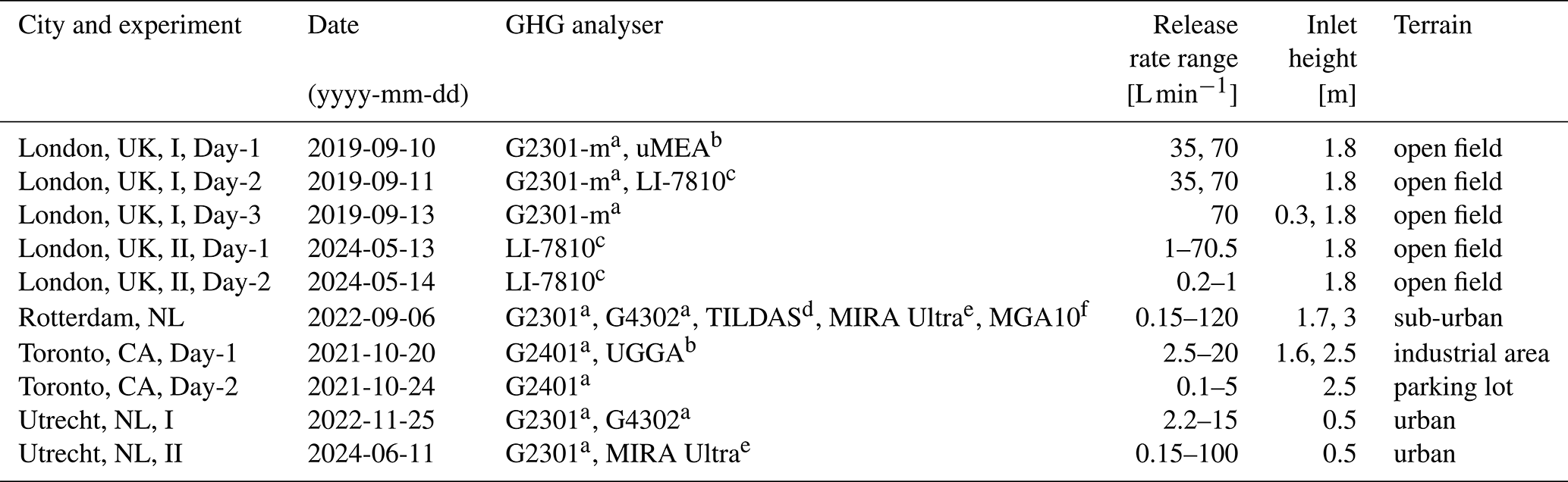
Figure 1a shows that the comparison of measured peak maxima among different instruments reveals very strong systematic discrepancies. Compared to the G4302, all other instruments (MIRA Ultra, G2301, MGA10, and TILDAS) strongly underestimate the peak maximum. Specifically, the maxima recorded by the TILDAS are only half of those measured by the G4302, while the MIRA Ultra, G2301, and MGA10 show peak maxima that typically are only between 10 % and 30 % of the G4302 readings. Figure 1b shows that the evaluated spatial peak areas are much more consistent between instruments, with slopes between 0.44 and 1.01. The coefficient of determination R² is notably higher for the area fit when compared to the maximum fit for all instruments. R² for G2301_U, MIRA Ultra, and TILDAS exceeds 0.96. The MGA10 device stands out as an exception, as it demonstrates poor R² values for both maximum and area fits. Both measured maximum and area values are more scattered and exhibit strong deviations from the other instruments. Interestingly, the G2301 analyser aligns better with the G4302 for data collected in Utrecht than in Rotterdam (indicated by a higher slope). This reflects the better alignment of instrument measurements for smaller peaks; in Rotterdam, very high release rates were included. A similar pattern arises for the evaluation of the CREs in London I (Fig. S21). Both the uMEA and LI-7810 instrument measurements align more closely with G2301 measurements when assessing spatial peak area rather than peak maximum.

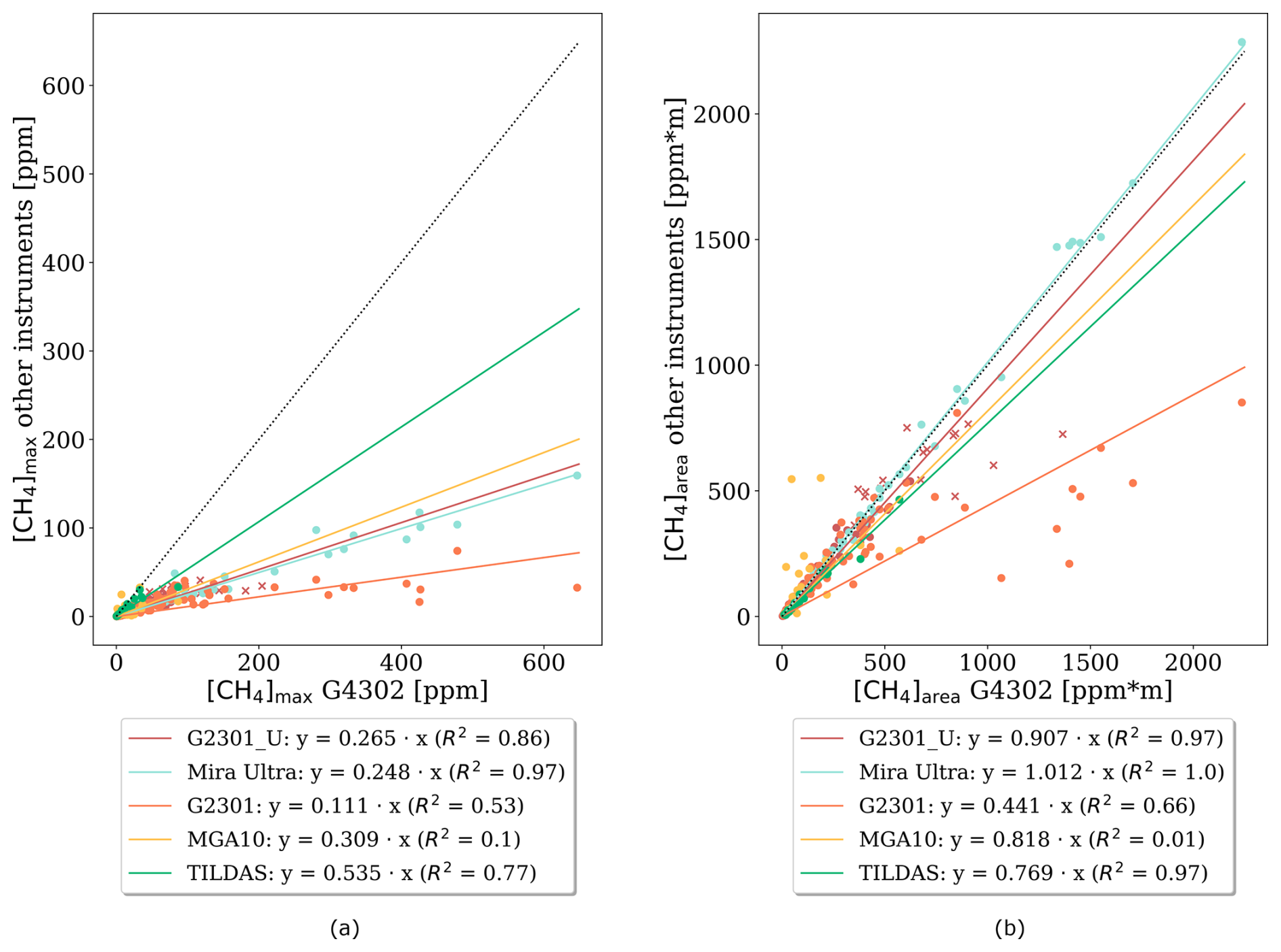
Figure 1 Comparison of (a) peak maximum and (b) spatial peak area from different instruments deployed in Rotterdam and Utrecht I (subscript “_U”): shown are the data points and a linear regression fit with intercept 0 for each instrument. The results from the G2301, MIRA Ultra, MGA10, and TILDAS devices are plotted on the y axis and the results from the G4302 instrument on the x axis. The dotted black line represents the 1:1 line. (For the G2301 analyser, peaks exceeding a maximum of 20 ppm are marked with an “x” and excluded from the fitting process.)

Our analysis demonstrates that different CH₄ analysers show much better consistency in the integrated CH₄ spatial peak area compared to the maximum CH₄ enhancement. This finding is supported by conceptual considerations: measured mole fractions are influenced by instrument characteristics, mainly flow rate, cell volume, and measurement frequency (Fig. 2). A higher flow rate or smaller cell volume will generally make measured mole fraction profiles sharper and higher. Lower flow rates and larger cell volumes, on the other hand, lead to smoothing effects, rendering the CH₄ peak smaller and wider (Takriti et al., 2021; Maazallahi et al., 2023). While the peak maximum is strongly affected by these characteristics, the integrated area is not. Each molecule that enters an instrument is measured, as part of either of a wide and low or a narrow and high peak. Gillespie et al. (2023) and Maazallahi et al. (2023) made similar observations when comparing different analysers. In this study, we generalize these results by demonstrating the same effect across eight different instruments, enhancing the robustness of this conclusion. Beyond differences in instrument performance, Ars et al. (2020) noted the area to be more robust against differences in inlet height, further supporting the argument for using the integrated spatial peak area as a more reliable metric for quantifying CH₄ enhancements. In future mobile surveys, several different instruments are expected to be deployed to survey local natural gas distribution networks. It is therefore important to move beyond the maximum enhancement as an emission estimation metric and use the spatial peak area instead.

Figure 2 Influence of the instrument characteristics (a) flow rate, cell volume (depending on cell temperature and pressure), and (b) measurement frequency on the peak shape detected.

3.2 Converting spatial peak areas to emission rates

Figure 3b shows the recorded spatial peak areas as a function of the known release rates (double logarithmic axes) from all controlled release experiments. As anticipated, higher CH₄ release rates, in general, correspond to higher observed spatial peak area measurements. A linear fit can be applied to these data, and the fit equation is proposed as an empirical model relating integrated spatial peak area of CH₄ enhancements (${\left[{\mathrm{CH}}_{\mathrm{4}}\right]}_{\mathrm{area}}$, in ppm ⋅ m, background levels subtracted from CH₄ measurements) to emission rates (r_E, in L min⁻¹):

$$\begin{array}{}\text{(11)}& \ln \left({\left[{\mathrm{CH}}_{\mathrm{4}}\right]}_{\mathrm{area}}\right)=\mathrm{0.774}\cdot \ln \left(r_{\mathrm{E}}\right)+\mathrm{1.84}.\end{array}$$

In practice, emission rate estimations will be derived from area measurements. To achieve this, Eq. (11) can be solved for r_E as follows:

$$\begin{array}{}\text{(12)}& r_{\mathrm{E}}=\exp \left(\mathrm{1.292}\cdot \ln \left({\left[{\mathrm{CH}}_{\mathrm{4}}\right]}_{\mathrm{area}}\right)-\mathrm{2.377}\right).\end{array}$$

The natural logarithm of the spatial peak area associated with a leak indication can then be inserted in the equation. If multiple transects were taken, the average logarithm of the spatial peak area values $\stackrel{\mathrm{‾}}{\ln \left({\left[{\mathrm{CH}}_{\mathrm{4}}\right]}_{\mathrm{area}}\right)}$ corresponding to the same leak indication should be used.

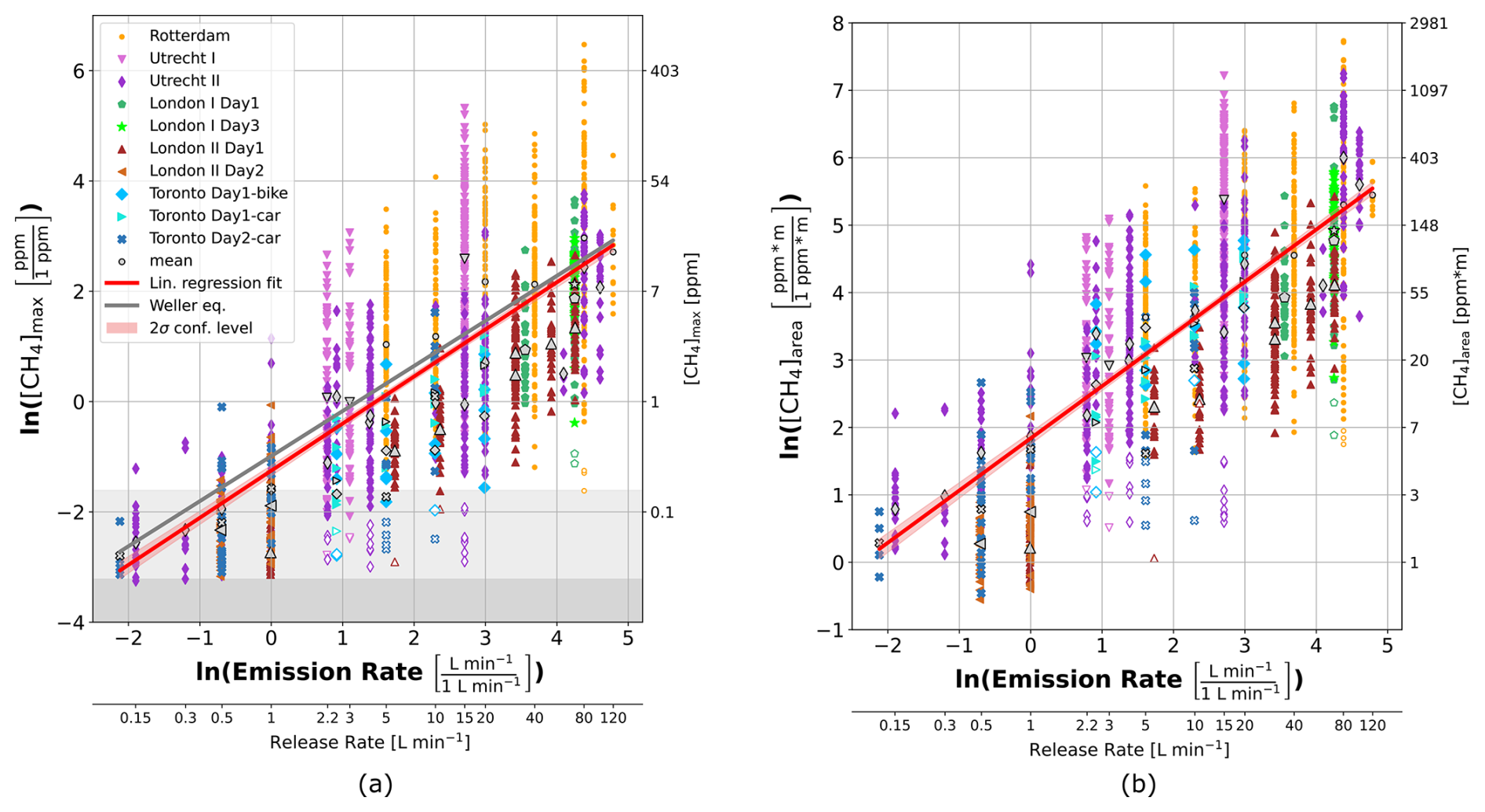
Figure 3 Correlation of the natural logarithm of (a) the peak maximum enhancement and (b) spatial peak area with the natural logarithm of the release rates for all controlled release experiments reported in this paper (except London I Day 2). Different cities are indicated by different colours (Rotterdam – orange, Utrecht I – pink, Utrecht II – dark purple, Toronto – blue, London I – green, and London II – brown). Black markers indicate mean values per release rate and city and unfilled markers indicate potential outliers. The second x axis indicates release rates deployed and the red lines are linear regressions to all data. The Weller equation (grey line in panel a) is displayed as a comparison and the light (dark) grey area indicates peaks below 110 % (102 %) of background level.

A similar linear regression fit was applied to peak maxima data: $\ln \left({\left[{\mathrm{CH}}_{\mathrm{4}}\right]}_{max}\right)=\mathrm{0.854}\cdot \ln \left(r_{\mathrm{E}}\right)-\mathrm{1.25}$ (Fig. 3b). The inferred regression equation for the maximum shows good agreement with the model proposed by Weller et al. (2019).

3.3 Using survey data for repair prioritization

A wide range of peak maxima and areas is observed for each release rate. This illustrates the shortcomings of the quantification of emissions for individual leak indications using this simple statistical method. This spread reflects the nature of turbulent dispersion of plumes. Environmental factors, in particular the built environment and meteorology, e.g. convection, complex wind patterns within urban areas (back circulation, wind channelling, and blockages), turbulence, and diffusion, play a major role in determining the location, shape, and CH₄ mole fraction of the meandering CH₄ plume (Carpentieri and Robins, 2015; Cassiani et al., 2020; Raz̆njević et al., 2022). Still, a greater CH₄ release increases the likelihood of detecting higher CH₄ mole fractions. This is the relation that is captured in the proposed transfer equation. Yet, changing wind conditions or turbulence can still cause the main plume to become highly diluted or be transported away from the street, leading to smaller peak maxima and spatial peak areas. At the extremes, high CH₄ mole fractions are measured in one transect and no peak at all in another one (Luetschwager et al., 2021). Ideally, measurements should be conducted downwind of the emission source and perpendicular to the wind. This approach is commonly used when targeting individual emitters, such as oil and gas processing stations or farms (Hensen et al., 2006; Korbeń et al., 2022). However, when measuring emissions from urban gas distribution networks, the built environment imposes constraints on positioning. Incorporating wind measurements from the survey vehicle could potentially improve emission estimates and should be explored in future research.

Additionally, some assumptions underlying the application of a linear regression are partially violated (homoscedasticity, normal distribution of errors). However, the premises were deemed sufficiently met to justify the use of linear regression, allowing for a straightforward and practical statistical inference model. However, as all experiments included in this study were executed during daytime (measurements were conducted between 09:00 and 18:00 local time), the method might not be suitable for the evaluation of nighttime measurements. During the night, the atmospheric boundary layer becomes more stable, which suppresses updrafts and leads to an accumulation of CH₄ emissions at the surface. This causes higher measured mole fractions, increasing both the peak maximum and spatial peak area measurements and hence most likely resulting in a considerable overestimation of the emission rate.

Similarly, though to a lesser extent, variations in solar irradiation during the day can influence updraft behaviour. Around noon, stronger solar irradiation is expected to enhance updrafts, which could reduce ground-level methane concentrations. Only a few release rates were deployed twice on the same day, preventing a conclusive analysis of measurement comparisons at different times. We recommend that future experiments investigate diurnal effects more systematically.

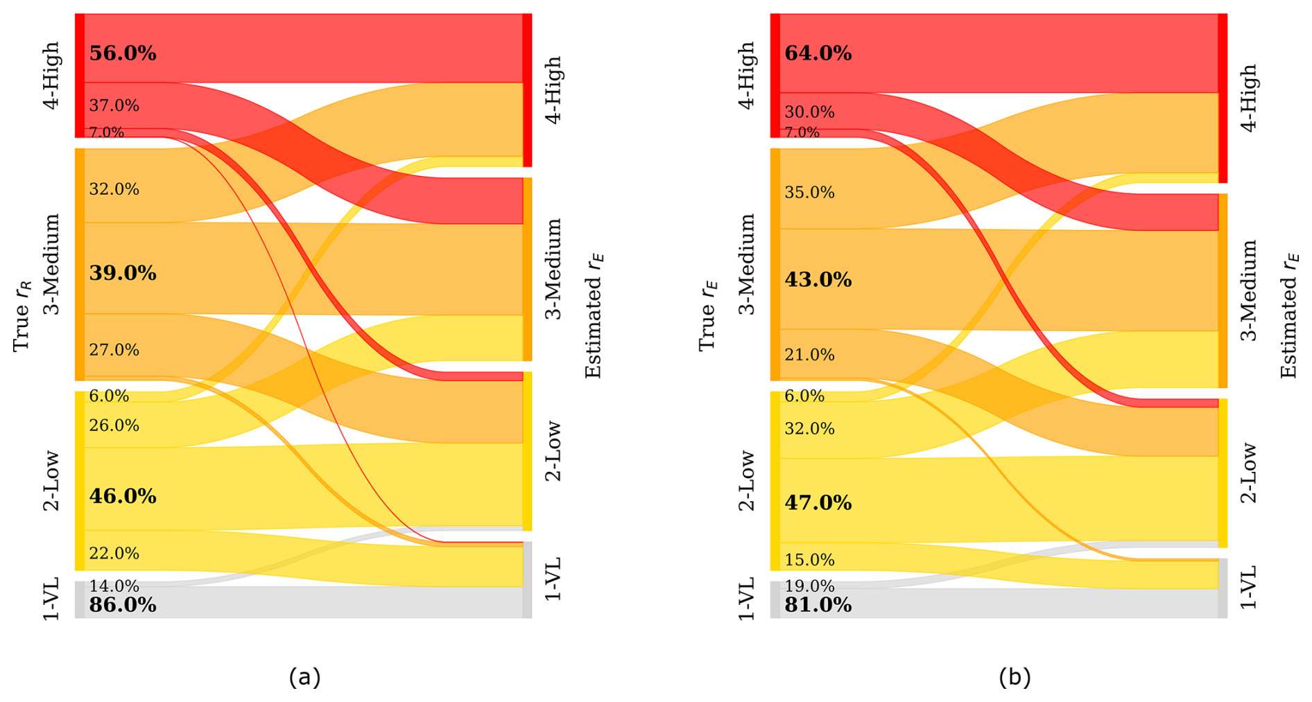
Figure 4 Categorization performance of (a) the Weller and (b) area method (including data from all six controlled release experiments). The left y axis represents the true emission rate r_E, where the width of the bars indicates the number of plumes belonging to each emission category (categories: 1 – very low, 2 – low, 3 – medium, and 4 – high). The right y axis represents the categories estimated by the statistical model, and the connecting lines visualize the amount of plumes (in %) from each category pool which the algorithm classifies into another (or the same) category.

Deviation of emission rate estimation from true emission rate can be very high for an individual gas leak, especially for single transects. For our set of experiments, under- and overestimation range from −100 % to +2700 %. To facilitate a pragmatic repair prioritization, categorizing leaks can be an important tool. We quantified the emission rate of all leak indications and subsequently assigned them to one of the four categories described above. Figure 4 illustrates the categorization performance based on quantification using the spatial peak area (a) and peak maximum (b). It displays the percentage of peaks correctly classified (bold number) and also shows in which categories the rest is falsely overestimated or underestimated. A suitable benchmark for categorization is a 25 % accuracy rate, reflecting the expected success when peaks are randomly assigned to one of the four categories.

The majority of very low and high peak indications are correctly attributed. Peaks in the medium category are less well classified, with a large portion being either over- or underestimated. Overall, the proportion of peaks that are misclassified by more than one category is very low. Around 7 % (22 %) of category 4 (3) peaks are underestimated into category 1 or 2 when applying the area equation. This means that the vast majority (78 % to 94 %) of higher emission peaks from categories 3 and 4 are correctly identified as medium–high, effectively differentiating them from low emission peaks. At the same time, 38 % (0 %) of category 2 (1) emission rates are falsely identified as high emission rates. The same analysis using the Weller equation yields comparable results, with a slightly lower categorization performance except for the lowest emission category (Fig. 4a).

It is important to note that these categorization performance rates vary across our set of release locations and are therefore not directly transferable to any leak populations in urban areas. The quantification and categorization performance differ for different locations; for example, the categorization precision for the London I data is 62 % for category 4 but 88 % for category 3, much higher than for the average (Figs. S22 and S23). Given the local circumstances regarding the built environment and meteorological conditions, peak measurements can be systematically lower or higher compared to the mean of our dataset. However, the numbers can still be considered as an indication of typical categorization performance.

In von Fischer et al. (2017), a categorization success rate of over 80 % for categories 2 and 3 was reported, which is higher than for our dataset. For the highest category, their performance was lower (38 %) than ours (64 %). The differences might be due to the specific local conditions where their controlled release took place. In practice, > 80 % of urban leaks have a low emission rate (von Fischer et al., 2017; Maazallahi et al., 2020) (category 1 was not assessed in those publications).

Overall, our results show that the categorization approach for leak repair prioritization would perform far better than making repair decisions by chance. Therefore, this approach offers the potential to reduce emissions, since larger leaks can be targeted first. The area equation does not consistently outperform the Weller model in terms of categorization performance, but it yields more consistent results across different instruments, which would facilitate the comparison of measurement surveys performed with different instruments.

3.4 Benefit of multiple transects

The discussed high uncertainty of individual estimations of the emission rate suggests that the performance may be improved by carrying out several transects. Including more measurements will reduce the random error associated with measurements and increase the confidence to capture the mean of this particular distribution (Cochran, 1977). This effect has been demonstrated in Luetschwager et al. (2021) and is illustrated in Fig. 5a. There, the Monte Carlo mean of the absolute percentage deviation of emission estimation, based on N transects ($N\in \left[\mathrm{2},\mathrm{10}\right]$), from the calculated mean emission rate based on all M transects measured for this release rate is shown. The percentage deviation from the mean decreases drastically with an increasing number of transects and converges to 0 for N = M (not shown). Note that here the absolute percentage error is displayed; no difference is made between a negative or positive deviation.

The observation that many of the mean values for individual release rates are still considerably different from the value expected from our conversion equation (Fig. 3) suggests that, in addition to random error, there is also a systematic error. This is likely due to the following two factors: the offset of the sample mean from the population mean (determined by longer-timescale weather phenomena) and the offset of the population mean from our linear regression (determined by the built environment).

Therefore, it follows that the error with respect to the true release rate will not necessarily decrease with more measurements for mean values that are far apart from the regression line. This is the case for the data from the London II experiment, which exhibit a large negative offset, as well as for the Utrecht I 15 L min⁻¹ release, which exhibits a very high positive offset (see Sect. S10 for a more detailed discussion). Still, if the offset is not too large, the error in emission estimation decreases with more transects. This is visualized in Fig. 5b, where the Monte Carlo mean of the absolute percentage deviation of emission estimation with respect to the true emission rate is shown.

The largest decrease in emission estimation error can be achieved from one to three transects, reducing the estimation error by one-third. A further decrease can be reached until around five–seven transects are included, after which the gained variation reduction levels off; including more transects then reduces the uncertainty by less than 3 %.

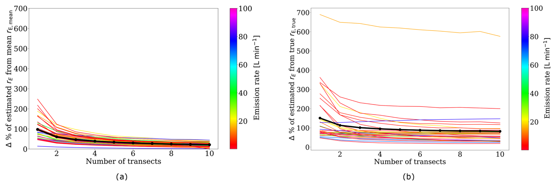
Figure 5 Mean absolute percentage deviation of emission estimation from the (a) calculated mean emission rate and (b) true release rate as a function of the number of transects. Each line represents one release rate at one location and was created by a Monte Carlo analysis with 2000 repetitions. The total mean over all release rates considered in this analysis is shown in black.

Luetschwager et al. (2021) carried out a similar analysis on multiple passages of real-world leak locations, comparing individual emission rate estimates to the emission rate estimate based on the distribution mean. They reported the sharpest decline in variation with increased detections from two to four, aligning with our analysis. They also noted that beyond five–six transects, the reduction in variability diminishes. Additionally, Luetschwager et al. (2021) reported errors relative to the mean of 50 % deviation based on two transects. This compares well with the variability in our corresponding analysis, which amounts to an average of 62 % for N = 2 comparing to the mean (Fig. 5a). Nevertheless, in comparison to true release rates from real measurements, the overall deviations are higher than in the aforementioned studies. We find the mean percentage deviation from the true release rate to be 115 % for N = 2 (Fig. 5b). Further, the deviations are skewed, with higher overestimations than underestimations, a result of the right-skewed distribution of measured spatial peak area values.

Raz̆njević (2023) stated that at least 10 transects are necessary to estimate the source strength within 40 % of the true emission, simulating a mobile measurement setup in a large eddy simulation model. We found, for half of the cases, an estimation error within 58 % when including 10 transects; for the other half, errors ranged between 65 % and 200 % with one outlier at over 500 %. Thus, our findings are in closer agreement with Raz̆njević (2023) than with the smaller estimation errors reported in Luetschwager et al. (2021). The generally higher estimation errors demonstrate the complexity of real-world environmental influences.

The persistent estimation error, even with the inclusion of more transects, likely reflects the influence of the built environment and meteorological conditions. If there is a systematic bias for that specific location or time frame of measurements, combining several transects will still include that high or low bias. Additional measurements can only balance out random errors or fluctuations. Taking measurements under different meteorological conditions could potentially improve estimations, enabling sampling of the full distribution of possible realizations of the emission plume.

Figure 6 illustrates that the accuracy of categorization on average improves when taking into account one (Fig. 6a), three (Fig. 6b), or six (Fig. 6c) transects. The London II and Utrecht I 15 L min⁻¹ releases are not included in this analysis because they include strong systematic biases. For emission rate estimations based on one single transect (N = 1), the categorization performance ranges between 47 % and 74 %, averaging 58 %. When three transects are used (N = 3), the categorization performance improves to an average of 65 %. Including six transects (N = 6) further enhances performance to an average of 69 %, ranging from 62 % to 82 %. More importantly, the number of strong over- or underestimations decreases. For example, whereas for only one transect, 5 % of category 4 peaks and 15 % of category 3 peaks are categorized as category 2, this reduces to 0 % and 5 % for six transects, respectively. Also, the false overestimation of 6 % of category 2 peaks into category 4 vanishes when increasing sampling effort to six transects.

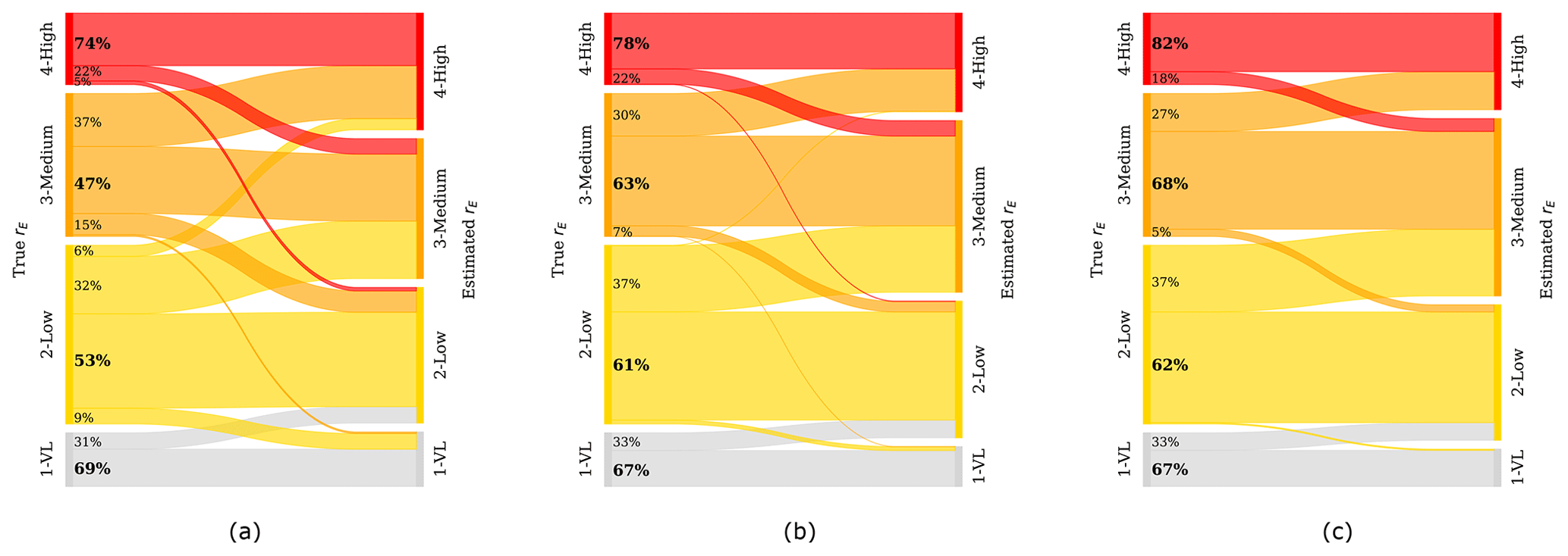
Figure 6 Categorization performance of the area equation with (a) N = 1, (b) N = 3, and (c) N = 6 transects for distributions with a small to medium offset (25 of the 35 release rates). The left axis represents the true r_E, where the width of the bars indicates the amount of plumes belonging to each emission category (categories: 1 – very low, 2 – low, 3 – medium, and 4 – high). The right axis represents the categories estimated by the statistical model, and the connecting lines visualize the number of plumes from each category pool which the algorithm classifies into another (or the same) category. The underlying dataset is based on the Monte Carlo simulation, resulting in 2000 estimates per release rate.

3.5 Suggested method for routine implementation of leak surveys

We suggest the following approach for routine mobile leak detection surveys in urban areas:

1. Survey. Perform surveys with an instrument that falls under the “1–1–10 principle” – at least 1 Hz measurement frequency, 1 s residence time, and 10 ppb precision. Record GPS data together with the mole fraction measurements, ideally with the same measurement frequency as the CH₄ analyser. Ensure that the GPS and CH₄ recordings are time-synchronized. Measure and record the inlet delay time for the CH₄ measurements at the beginning of the survey. Optimally, gather wind measurements as well, such as with an anemometer mounted on the vehicle's roof. If possible, maintain a sufficient distance from previously passed cars while conducting the measurements. During the survey, if an enhancement above the CH₄ background exceeds 0.2 ppm, attempt to conduct six transects downwind of the leak indication.

2. Evaluation. After the survey campaign, determine CH₄ background levels and subtract them from the CH₄ measurements (CH₄ background at a certain time = 10th percentile of CH₄ mole fractions within a ±2.5 min time window). Use a peak detection algorithm to identify peaks in the time series, including the start and end times of each peak. If available, use additional information such as ethane measurements, methane : carbon dioxide ratio, or CH₄ isotopic composition to differentiate between biogenic, combustion, and fossil sources. Use GPS data to infer the driving speed to convert the time series to space coordinates and calculate spatial peak areas (using the CH₄ elevation above background levels). In case several transects were done for the same leak indication, take the average of the $\ln \left({\left[{\mathrm{CH}}_{\mathrm{4}}\right]}_{\mathrm{area}}\right)$ of the individual peaks detected during the different transects. Calculate the emission rate by inserting the $\ln \left({\left[{\mathrm{CH}}_{\mathrm{4}}\right]}_{\mathrm{area}}\right)$ value into the inverse area equation (Eq. 12).

3. Categorization. Rank the leak into one of the four emission categories (< 0.5 L min⁻¹ – very low, 0.5–6 L min⁻¹ – low, 6–40 L min⁻¹ – medium, and > 40 L min⁻¹ – high) and use this categorization in addition to safety concerns to prioritize leak repair efforts.

4. Report. Report the number of leaks per category and the number of leaks per pipeline kilometre. Report the leak size distribution and total emissions for the surveyed area. Ideally, provide these numbers separately for different pipeline materials (e.g. cast iron, steel, polyethylene, and PVC).

4 Conclusions

Our results clearly highlight systematic differences in maximum CH₄ enhancement recorded by different commercial CH₄ gas analysers. Maximum enhancements differ by up to a factor of 10 between instruments. When the spatial peak areas are evaluated, differences between instruments reduce to less than a factor of 2, confirming our hypothesis that the spatial peak area is a more suitable quantity than the recorded peak maximum. We suggest moving beyond the peak maximum as an emission estimation metric to avoid biased emission predictions.

We propose an empirical equation for the emission rate (r_E, in L min⁻¹) based on the integrated spatial peak area of CH₄ enhancements (${\left[{\mathrm{CH}}_{\mathrm{4}}\right]}_{\mathrm{area}}$), in ppm ⋅ m, background levels subtracted from CH₄ measurements:

$$\begin{array}{}\text{(13)}& r_{\mathrm{E}}=\exp \left(\mathrm{1.292}\cdot \stackrel{\mathrm{‾}}{\ln \left({\left[{\mathrm{CH}}_{\mathrm{4}}\right]}_{\mathrm{area}}\right)}-\mathrm{2.377}\right).\end{array}$$

Here, $\stackrel{\mathrm{‾}}{\ln \left({\left[{\mathrm{CH}}_{\mathrm{4}}\right]}_{\mathrm{area}}\right)}$ is the mean taken over several transects associated with the same leak indication. This formula is very simple in deployment; it does not require any additional information other than the actual CH₄ mole fraction and GPS measurements. However, it therefore ignores other important local influences. The most important parameters are likely the built environment, wind speed and direction, atmospheric stability, and turbulent processes. It is expected that incorporating parameters reflecting those factors could improve emission rate predictions. However, especially when it comes to incorporating turbulent processes, the associated measurement effort would become extensive. Therefore, the strength of our simple statistical model is the simplicity of its implementation, still providing reasonable emission estimates. Higher sampling effort can improve quantification accuracy significantly. Including three transects instead of one improved correct categorization into four emission categories from 47 %–74 %, to 61 %–78 %, and to 62 %–82 % when incorporating six transects instead of one transect. Thus, applying this method to identify, quantify, and prioritize leak repairs in urban natural gas distribution systems can support greenhouse gas emission mitigation during the transition to a fossil-fuel-free energy system.