Expanding observational capabilities of diode-laser-based lidar through shot-to-shot modification of laser pulse characteristics

A method for expanding the observational capabilities of diode-laser-based atmospheric lidar is discussed. A straightforward test, consisting of interleaved “Long” and “Short” laser pulses, is developed to demonstrate how shot-to-shot modification of laser pulse characteristics can enhance the performance of low-power, diode-laser-based lidar and could benefit atmospheric observations. Two examples are given to demonstrate the technique. In the first, water vapor profiling is extended closer to the surface while simultaneously maintaining sufficient far-range performance. These results are verified with collocated measurements. In the second example, clouds are resolved at high vertical spatial resolution with a high signal-to-noise ratio. Details of the lidar instrument hardware and the method to combine the laser pulses of different durations are given.

1 Introduction

Lidar observations have been used for a number of atmospheric science applications, including, but not limited to, process studies, weather/climate monitoring, and assimilation into numerical weather prediction models. While scientific applications are typically the ultimate goal, scientific advancements are often fostered by technological advancements. As such, much of the focus of research on modern lidar systems centers around lidar hardware, particularly the laser sources used. Different types of laser sources can be employed in lidar, depending on the desired measurement requirements. Historically, diode lasers have been primarily used in ceilometers but have expanded in their applicability in recent years to more quantitative lidar systems such as differential absorption lidar (DIAL) (Nehrir et al., 2011) and high-spectral-resolution lidar (HSRL) (Hayman and Spuler, 2017). Diode lasers are effective laser sources for these types of quantitative lidar because they are cost-effective, are robust, are available at a large number of wavelengths, have a narrow bandwidth, and are flexible in their operational parameters. In contrast, the prime drawback of diode lasers is their low peak power.

Roughly a decade ago, the potential for quantitative atmospheric lidar systems based on diode lasers was first demonstrated (e.g., Nehrir et al., 2011; Repasky et al., 2013; Hayman and Spuler, 2017). The benefit of a diode-laser-based lidar architecture stems from higher reliability and lower-cost systems, not from their pure performance vis-à-vis output power. For high-power atmospheric lidar systems, solid-state lasers are typically used (e.g., Nd:YAG, Ti:Al₂O₃, or Alexandrite) (e.g., Thayer et al., 1997; Goldsmith et al., 1998; Eixmann et al., 2015; Wulfmeyer, 1998; Strotkamp et al., 2019). In contrast, diode lasers have relatively low peak power, on the order of watts – compared to hundreds of kilowatts or megawatts from solid-state lasers. As part of a compensating mechanism, diode-laser-based lidar systems have typically used relatively long pulse lengths, on the order of hundreds of nanoseconds to microseconds.

Generally, for a coaxial monostatic lidar system, the lidar system is blind when the laser pulse is outgoing. Detector recovery time can add to this blind zone. For typical high-power solid-state lasers, the pulse durations are short (on the order of nanoseconds), and the blind period imposed by the pulse itself is practically irrelevant, leaving only detector recovery time to impact the dead time. However, for diode-laser-based lidar, there is a direct trade-off. Longer pulses, having more average power, enable long-range observations but sacrifice near-range observational capability. Shorter pulses, in contrast, can be used to see at nearer ranges and at higher range resolution but lack the average power to see to greater distances.

Although diode lasers have relatively low peak power, they enable more flexibility, modularity, and agility than conventional solid-state lasers. The concept to be explored in this work is to leverage that flexibility – to simply transmit multiple outgoing laser pulse lengths, altering laser parameters from shot-to-shot, to expand the observational range and resolution of diode-laser-based lidar systems. This has the benefit of allowing for rapid changes in observational sensitivity, with longer pulses used to see to further ranges and shorter pulses used to see to closer ranges, and enabling higher-resolution observations within dynamic targets, such as clouds. Although the concept of altering pulse characteristics from shot-to-shot as well as sub-pulse alterations (typically referred to as pulse compression) is well explored for radar hardware (e.g., Ramp and Wingrove, 1961; Mudukutore et al., 1998; O'Hora and Bech, 2007; Richards et al., 2010), to our knowledge, these techniques have not been adopted for use in atmospheric lidar. This is likely due to the limited flexibility of high-power solid-state lasers, where implementing such a capability would represent a significant engineering challenge. These lasers are best behaved in steady-state operation due primarily to thermal transient effects (Hooker and Webb, 2010). Altering operational characteristics, such as pulse length, pulse repetition frequency, or peak power, of most solid-state lasers significantly alters the thermal and refractive-index properties of the gain material. If not carefully mitigated, localized heating from the resultant thermal lensing can cause catastrophic damage to optical components. Although there are thermal effects for diode lasers, the relatively high wall-plug efficiency¹ and the comparatively lower peak power of diode lasers allow most of the energy input into the laser to leave as light, with localized heating minimized.

The primary contributions of this work are first to implement a timing unit on an atmospheric observing lidar system to allow for this shot-to-shot control of laser pulse characteristics, to our knowledge for the first time, and second to explore the enhanced observational capability of such a lidar system. The lidar hardware is briefly described in Sect. 2. The system used to perform the shot-to-shot alteration of laser characteristics is described in Sect. 3. The implementation of this system to expand the observational capability of this lidar system to measure water vapor is described in Sect. 4. A discussion of the ability to combine data from multiple pulse lengths is presented in Sect. 5. Finally, a discussion of the results, conclusions, and future work are given in Sect. 6.

2 MicroPulse differential absorption lidar (MPD)

The MicroPulse differential absorption lidar (MPD) used in this work uses a pair of DIAL systems. One DIAL operates near 828 nm and is used to measure water vapor absolute humidity, while the other DIAL operates at 770 nm and is used, with an embedded HSRL, to measure temperature. The MPD instrument and the most recent version of the laser system are described in Spuler et al. (2015) and Spuler et al. (2021), respectively, while the observations are described in Stillwell et al. (2020) and Hayman et al. (2024). There are two differences between the configuration presented in Spuler et al. (2015, 2021) and the one used for this work that should be noted. Additionally, while MPD consists of a pair of DIAL systems, we chose to focus on a single system, i.e., the water vapor system, for this work.

The first difference is in the optical hardware used to interleave the DIAL laser wavelengths. A trio of optical switches (a pair of 1×1 switches and a single 2×1 switch) are replaced with a pair of booster optical amplifiers (BOAs) that are operated in pulsed mode combined with a fiber optic coupler (Spuler et al., 2023). When the pulse current is applied, the BOA acts to amplify a continuous wave seed laser. When off, the amplifier acts as a strong absorber (effectively a closed switch). This pair of amplifiers is coupled with a passive fiber coupler to a tapered semiconductor optical amplifier (TSOA). The pulses from the BOAs are interleaved so that only one wavelength from each DIAL may fire at a time. The overall performance of this laser design is similar to the performance described by Spuler et al. (2021) with the benefits of being more stable, robust, temperature insensitive, and more cost-effective and having better cross-talk mitigation between wavelengths. A block diagram of this design is provided in Appendix A, Fig. A1, which can be compared to Spuler et al. (2021) Fig. 1.

The second difference is the replacement of the main clock that controls the timing of the laser and receiver systems. The clock used for the system described by Spuler et al. (2021) was an eight-channel pulse generator (Quantum Composer 9530). This pulse generator served as the master clock for the lidar system. This pulse generator provided a consistent input to the lidar system, i.e., making the lasers operate at steady state. The replacement is a custom field-programmable gate array (FPGA)-based pulse generator, which is described in more detail in Sect. 3. This custom FPGA-based pulse generator provides all of the same electrical connections but allows for shot-to-shot changes in laser timing.

3 Primary timing unit

The FPGA-based timing unit consists of a commercial off-the-shelf single-board computer module (control board) connected to a custom-built interface printed circuit board (interface board). The control board is based on a Xilinx Zynq System-on-Chip. This chip combines an FPGA and an ARM CPU capable of running embedded software. A combination of software and FPGA firmware implements the required control functions. The custom-built interface board converts electrical signals from the control board to provide TTL-like (TTL: transistor–transistor logic) output to each of MPD's DIAL laser pairs (each consisting of one TSOA and two BOAs), detectors (consisting of three identical avalanche photo diode gate signals), and signals to the MPD acquisitions system (one trigger, one binary flag to indicate which laser, online or offline, is firing, and a binary flag indicating the pulse width).

The FPGA timing unit allows for the definition of multiple pulsing schemes and can switch from one scheme to the next in a single FPGA clock cycle (in this case, 5 ns). The definition of each pulsing scheme, which we will refer to as pulse blocks or simply “blocks”, includes individual definitions for the inputs provided by the original master clock, definitions of the pulse repetition time, the total number of pulses to fire, the split between the two DIAL wavelengths, and the amount of time to wait after completion of each definition. Each of the inputs provided by the new master clock is defined in one of two ways: as a pulse or as a binary value. Each pulse is defined by three numbers: a pulse length, a delay, and an On-Off keying sequence. The intention of the pulse delay is to account for any rise times or any electrical delays that would be required to synchronize components, while the On-Off keying sequence is to allow for intra-pulse modulations.

This timing unit was born out of a design used for the NSF NCAR HIAPER Cloud Radar (Vivekanandan et al., 2015). Some of the features are unused in this work but are described and noted for future capability enhancement. Specifically, the amount of time to wait after completion of each block allows for different unambiguous ranges for each pulse block and provides block-to-block control of the pulse repetition frequency (used in Doppler radar for velocity unfolding). The On-Off keying is intended to allow intra-pulse modifications such as would be necessary to implement radar-style pulse compression by intra-pulse phase modulation.

For this work, we specified three blocks (of the 32 possible), as defined in Table 1. The first block we refer to as “Long”, the second “Short”, and the third “Very Short”. Henceforth, quotation marks are ignored, with names identified by their capitalization. The Long block defines the MPD settings needed to fire 1 µs laser pulses, whereas the Short and Very Short blocks are the settings for 0.2 and 0.1 µs pulses, respectively. The Long block is chosen because it mimics the operational settings used for previous MPD observations (Spuler et al., 2015, 2021; Stillwell et al., 2020; Hayman et al., 2024). Each block fires two shots, one with the online laser and one with the offline laser for each DIAL pair, which are synchronized. This creates a series of four laser pulses before the system repeats. The laser output rate is 8 kHz – 2 kHz effectively for each pulse type (Online Long, Offline Long, Online (Very) Short, and Offline (Very) Short). This is shown in Fig. 1.

Table 1 Clock settings used for this work. The timing unit is set to switch between blocks upon completion of pulsing defined by the “Number of pulses”. Note that all On-Off keyed sequences are disabled for this work.

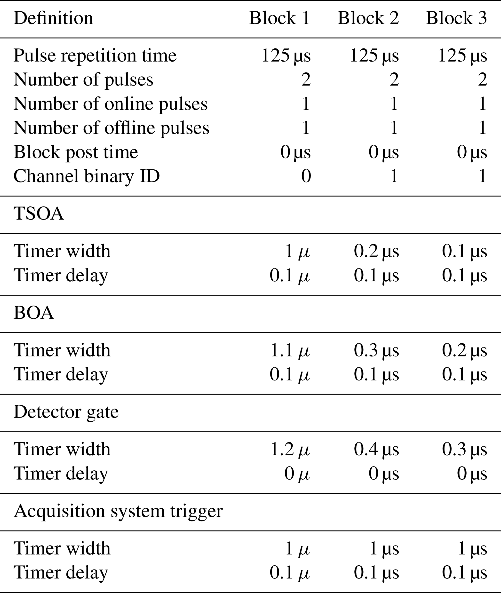
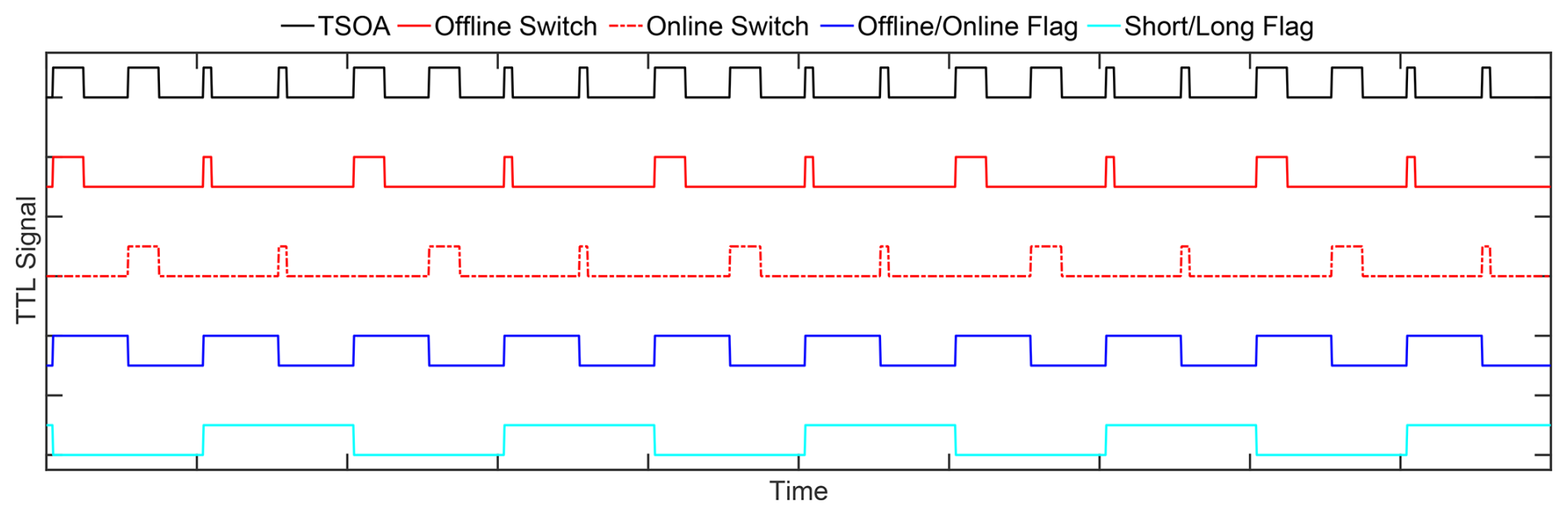
Figure 1 Timing diagram of the interleaved Long and Short modes defined in Table 1. The “Switch” signals are the drive current to the BOAs. Timing is to scale, except that pulses are intentionally enlarged by a factor of 40 for illustrative purposes. The bottom two signals are used as binary signals into the MPD acquisition system to parse out the data from the single water vapor detector to one of four acquisition channels, where 00 = Offline Long, 01 = Offline Short, 10 = Online Long, and 11 = Online Short.

4 Water vapor observations

NSF NCAR operates a network of five MPD systems. One of these instruments (MPD04) was equipped with the timing unit described in Sect. 3 and deployed at the NSF NCAR Marshall Field Test Site near Boulder, Colorado (39.95° N, 105.196° W) in fall 2024 (NCAR/EOL-MPD-Team, 2020). The MPD was run unattended from 16 October to 2 November 2024. A total of nine collocated radiosondes were launched at the Marshall Field Site. MPD was run with the timing shown in Fig. 1, with an even split between Short pulses and Long pulses.

MPD observations (photon counts) were processed using the method of Stillwell et al. (2020), which itself is largely a restatement of the method originally defined by Spuler et al. (2015). Spectroscopic calculations were performed following the method of Hayman et al. (2019) trained with data from HITRAN2020 (Gordon et al., 2022). Error estimates were calculated using the bootstrapping method defined in Spuler et al. (2021). Note that radiosondes measure relative humidity, whereas MPD measures absolute humidity. To compare the two observations, the relative humidity of the radiosondes was converted to absolute humidity using the saturation vapor pressure calculated using the approximation method of Lowe (1977). The saturation vapor pressure was then converted to number density using the ideal gas law.

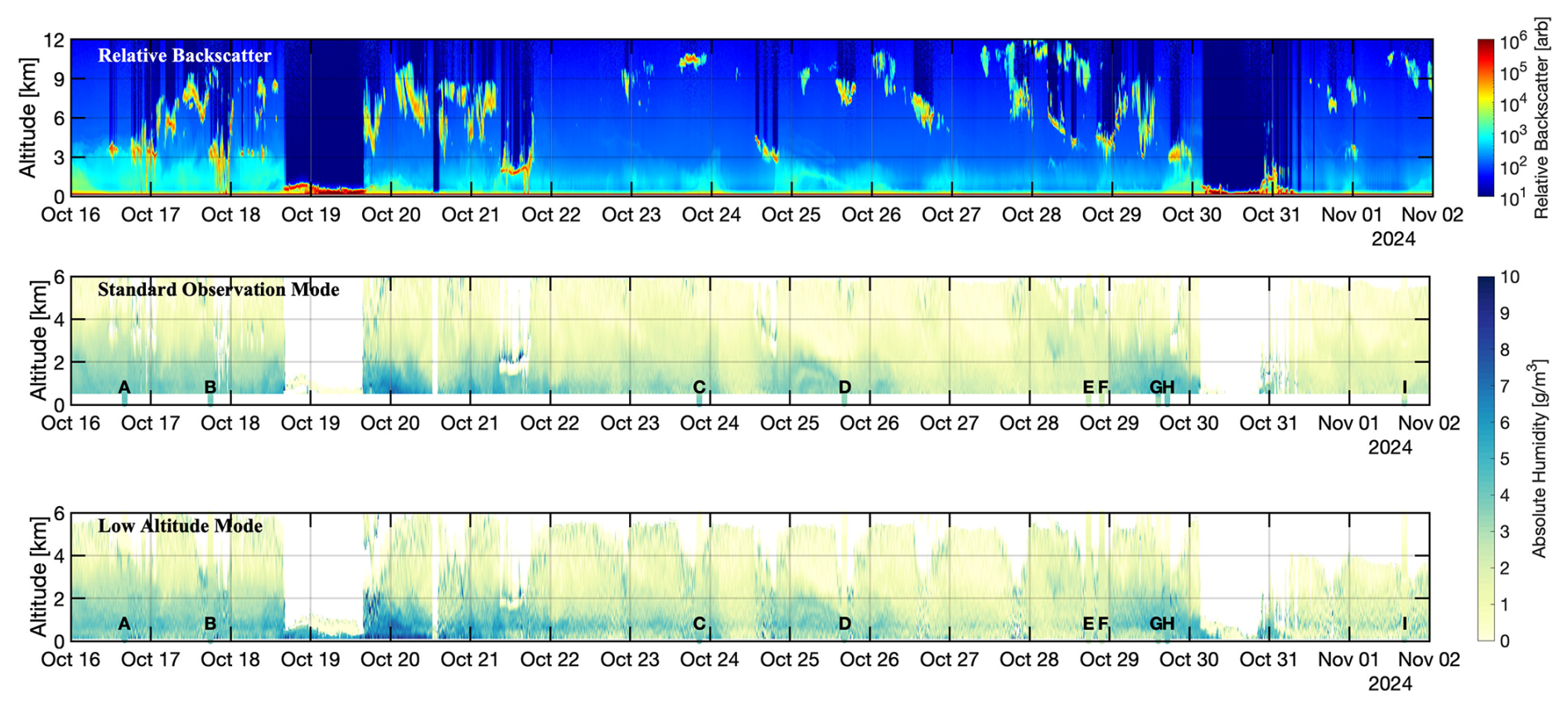
Figure 2 MPD data taken from 16 October 2024 through 1 November 2024. Water vapor measurements from the “Standard Observation” (Long pulse) and “Low Altitude” (Short/Very Short pulse) modes are taken per the settings in Table 1. Radiosonde data are overlaid on the water vapor panels, with letters corresponding to the panels in Fig. 3. Relative backscatter is given for context to identify where clouds are blocking the lidar signals and where high background levels from clouds are to be expected. All radiosonde labels are at the same altitude for context to identify the minimum observable altitude for standard observations.

Absolute humidity and relative backscatter are shown in Fig. 2. Radiosonde data are plotted on top of both MPD absolute humidity contours, each labeled with a letter corresponding to the respective panel in Fig. 3. Relative backscatter originating from the Long laser pulses is given for context where the stronger signals are mostly clouds. The “Low Altitude Mode” shown in Fig. 2 consists of the Short pulse block from 16 October to the middle of the day on 30 October. It was changed for the last 2 d to the Very Short pulse block.

There are a couple of things to note about Fig. 2. First, it is generally difficult to differentiate the MPD absolute humidity from those observed from the sonde; the easiest place to see a difference is in the lower 500 m of the Long pulse observations, where MPD data are absent. This is expected given the extensive validation of the instrument and the quantitative nature of the DIAL method (Weckwerth et al., 2016; Spuler et al., 2021). What is noteworthy is that operating the system in two pulse modes has not proved detrimental to the original instrument performance, less the decline in performance that results from using effectively half the laser pulses in a given time period. Second, the Long pulses generally have data that extend further in range than the Short pulses. This is due to the higher average output power of the Long pulses increasing the observed signal-to-noise ratio (SNR). This is especially true during daylight hours, which are approximately 13:00 to 24:00 UTC, and even more prominent under daytime clouds, which have the highest rate of background light observations. It is also clear that after the change from the Short to Very Short pulse blocks, the Low Altitude Mode water vapor maximum range drops.

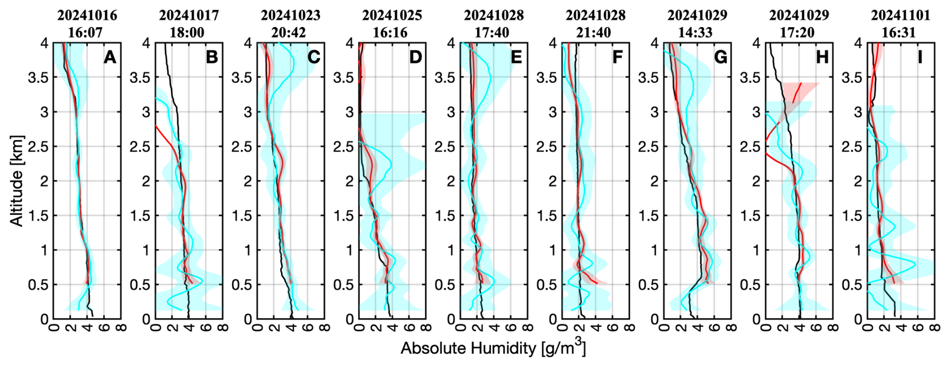
Figure 3 Comparisons of MPD WV data and collocated radiosondes (black) launched over the time period for Fig. 2. Red is the Long pulse mode, and cyan is the Short pulse mode for panels (a)–(h) and the Very Short pulse mode for panel (i). Solid lines are the retrieved values, with the shaded bars giving error estimates.

Figure 3 shows comparisons of the MPD data to the radiosonde data. The radiosonde data are given in black, and the MPD measurements are indicated by the solid lines, where red lines are Long pulses and blue are either Short or Very Short pulses. Shading of the same color is the measurement error estimate. There are three things that should be highlighted. First, the blue lines (either Short or Very Short pulses) extend significantly lower than the Long pulses; in this case, the minimum range is reduced from approximately 500 to 90 m. Second, of particular interest is the sonde shown in panel (g), which shows a relatively strong surface inversion, which is well captured by the MPD with shorter pulses. This inversion, if observed with longer pulses, is invisible. Using a method of inference, such as interpolation from the lowest range bin to the ground, would fail to show this feature, which could have consequences related to interpretation of the data. Third, in general, the error bounds are higher for the Short pulses than for the Long pulses. The optical paths for the transmitter and receiver of both pulse blocks are identical, as are the laser peak power and the background light. Long and Short modes therefore scale the signal-to-noise ratio of the measurement exclusively through output power, which in turn scales with the pulse length. The only notable caveat to this statement (that Long pulses have lower error) is at low altitudes, where measurements can be taken for Short pulses that are not possible for Long pulses. For Fig. 3, Short pulse errors (blue shading) are almost always larger than Long pulse errors (red shading). This is true at all ranges and times, but the errors are not constant because error bounds are strongly linked through the signal-to-noise ratio to the background count rate and, by extension, daytime cloud cover. Panels (a) and (g) occur under clear conditions, panels (c), (d), (e), and (i) occur under cirrus clouds, and panels (b), (f), and (h) occur under lower status clouds.

5 Sample observations

So far, we have treated data from the MPD's different pulse modes independently. We used direct retrieval methodologies to convert the MPD observations (photon counts) to water vapor absolute humidity, yielding two independent estimates. This is analogous to more traditional lidar systems that use observing channels of different sensitivity for low- and high-altitude observations. Examples include using two or more optical receivers with duplicate detectors (e.g., von Zahn et al., 2000; Reichardt et al., 2012; Newsom et al., 2020) or splitting the measured detector signal electrically (e.g., Newsom et al., 2009; Carroll et al., 2022). This leaves a number of natural questions including: (1) are the measurements necessarily equal? (2) If not, which measurement is more representative of the atmospheric state? (3) Can measurements be combined to yield a best guess of the atmospheric state? It is important to note that this set of questions is not unique to the methodology presented here and does not have a single universal solution.

Several methods have been proposed to answer these questions. Newsom et al. (2020) specify a fixed threshold whereby the far range channel is used above a set altitude, the low range channel is used below a second set altitude, and a linearly varying weighted average is used between those two altitude bounds. Carroll et al. (2022) specify something similar, where the data merge locations are not specified by altitude but by the observed optical depth. Forward models have also been shown to combine measurements of similar atmospheric variables with different sensitivity. For example, Löhnert et al. (2009) combine observations from passive remote sensors in the infrared and microwave, whereas Cadeddu et al. (2013) describe combining microwave remote sensors utilizing a pair of microwave water vapor emission lines with different opacity. The method of Marais and Hayman (2022) was used to forward-model MPD water vapor absolute humidity data. It uses data from only one sensitivity channel (in this case, our “Long” pulses), but it is theoretically extendable to two sensitivities. We elect to highlight this method in particular because it has already been applied to MPD data, but applying it to these data is beyond the scope of this work. Combining data in a robust manner should not be considered trivial. Presented here are two examples of measurements of differing sensitivity, one that is straightforward to combine and one that is not.

5.1 Combined water vapor retrievals

The method of data combination described by Newsom et al. (2020) is used with minor modifications to combine Long and Short pulse data from 29 October 2024, presented in Fig. 4. Datasets are merged with a linear weight beginning at 500 m and ending at 750 m, i.e., data below 500 m come exclusively from Short pulses, and data above 750 m come exclusively from Long pulses. Fig. 4 also shows the error estimate of the presented data both as an absolute and a relative error. These data were selected because of a relatively rare moisture inversion for the first half of the day that slowly dissipates. That feature is unique and stands out clearly on panel (g) of Fig. 3 but largely disappears 3 h later as shown in panel (h) of Fig. 3.

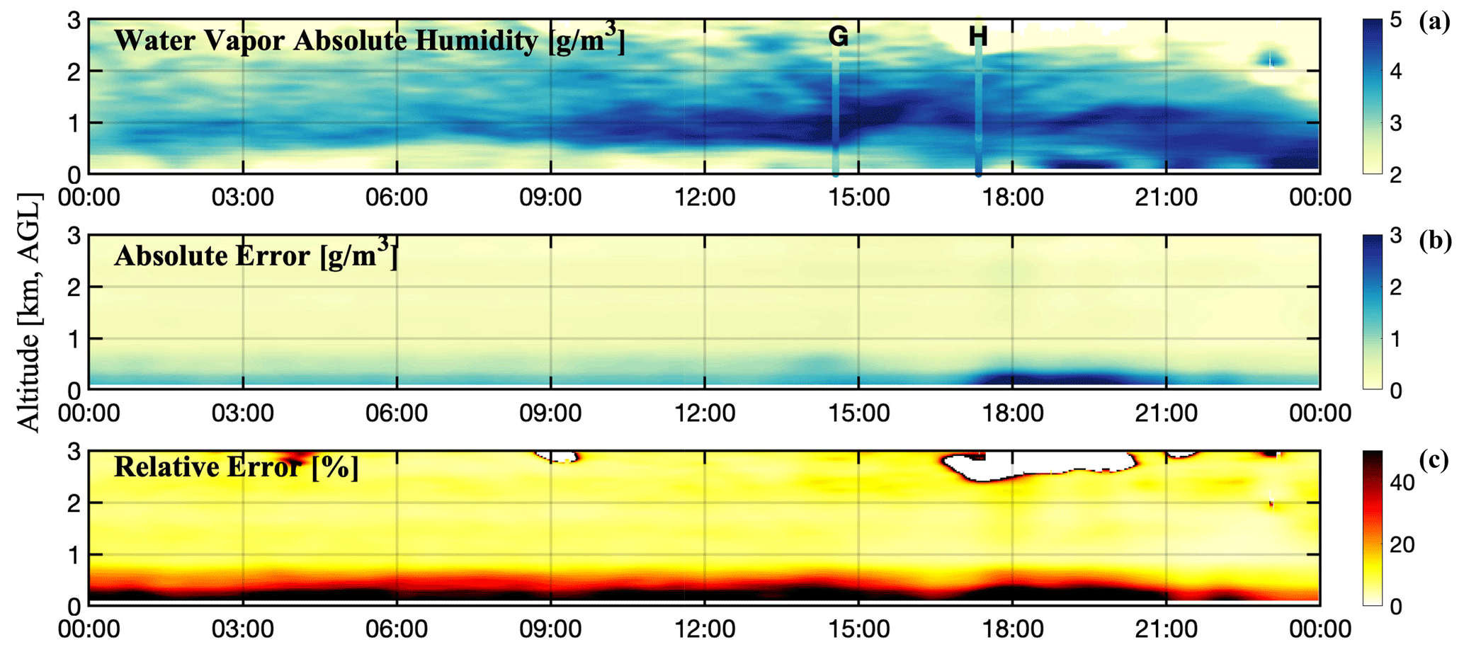
Figure 4 MPD data from 29 October 2024. Radiosondes overlaid on (a) correspond to panels (g) and (h) from Fig. 3.

Error estimates are provided in two ways because they highlight different components of DIAL-based moisture measurements. First, the absolute error for the Short pulses is naturally larger than that for the Long pulses, as shown in the middle panel of Fig. 4. This is first because Short pulses (≈1 µJ/pulse) are approximately 5 times less powerful than Long pulses (≈5 µJ/pulse) and second because, owing to poor overlap at short ranges, the MPD does not collect light as efficiently at near ranges as it does at far ranges, typical of most lidar systems. Absolute error spikes near 18:00 UTC correspond to background light enhancement caused by a cloud. Near 21:00 UTC, the cloud layer passes. This is basically hidden in the relative error contour because the error is rising due to background conditions, as the absolute humidity is rising due to the air mass changing during the observation. It is serendipitous that the magnitude of these two effects is almost the same. The relative error contour is helpful for identifying clouds in this case. DIAL observations typically show large biases within a cloud; as a result, most DIAL-based data near clouds and within clouds are masked. In this case, the bias is a strong dry bias. The absolute error estimate is quite low in clouds, not because the actual error is low but because the observed variance during bootstrapping is low due to this dry bias. There is not an enhancement in absolute error from the cloud at 09:00 UTC near the ground because the sun is not above the horizon; thus, the solar background observed is not enhanced by the cloud.

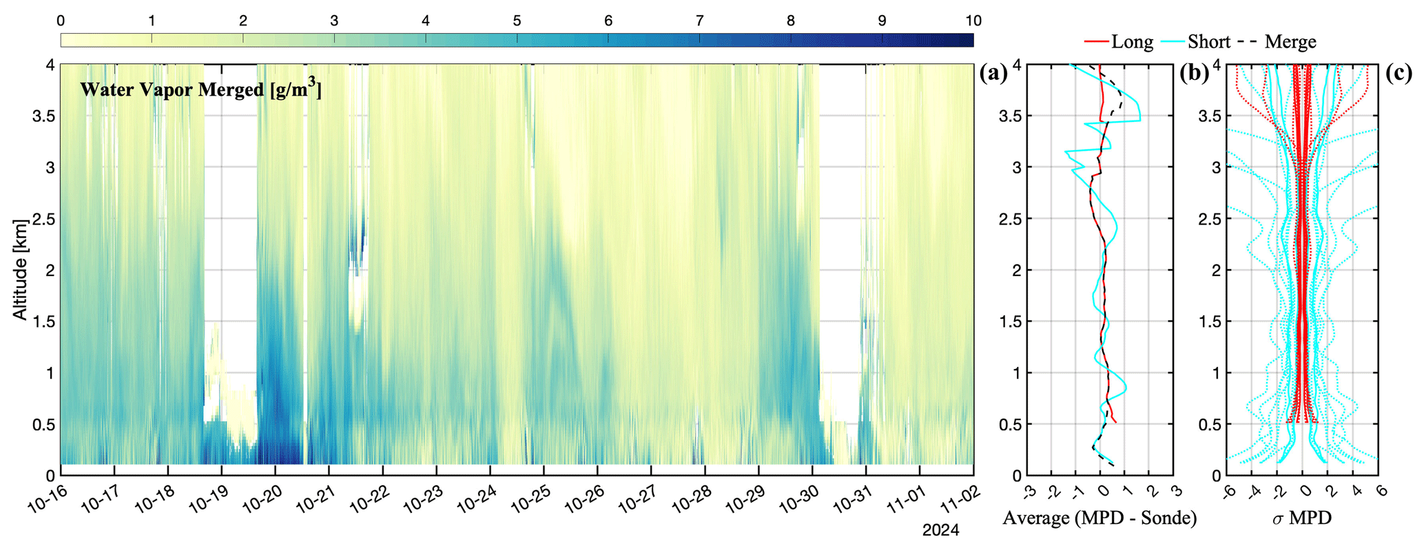
Figure 5 (a) Merged data product for the whole time period of Fig. 2. The average deviation of the merged product with the sondes shown in Fig. 3 is given in (b) and all the error bounds of the same sondes in (c). For those errors, solid lines occur under clear skies, and dashed lines occur under clouds.

Figure 5 displays the merged absolute humidity for the entire time period covered in Fig. 2. It also compares this merged product with all radiosondes and presents MPD error estimates at each sonde launch time. The abscissa for the sonde comparison spans half the range compared to the error estimates. A slight moist bias is evident for the Short pulses in both Fig. 2 and Fig. 5. This bias falls within the individual error bounds of each measurement and is reduced in the merged product because more information comes from Long pulses, which show reduced bias. It is noteworthy that the MPD system uses two telescopes combined by a fiber coupler. The observed bias occurs in the altitude range with the lowest overall signal levels. That is where the low-altitude telescope, despite reaching full overlap, begins to lose signal-to-noise ratio (SNR) with increasing range, while the far-range telescope has not yet achieved full overlap. This leads us to speculate that the bias is partly due to the low SNR, although the exact cause remains undetermined.

The error bounds for Short pulses are greater than for Long pulses. As expected, errors in cloudy conditions (dashed lines) are greater than in clear conditions (solid lines), owing to the increase in background light. Short pulses are expected to have larger error estimates than Long pulses because all operational conditions (e.g., background light levels, resolution, optical components, optical path of signal through optical components) are identical for both pulse types, except for the lower output power of the Short pulses. The Short pulse error asymptotically approaches the Long pulse error as signal photons go to zero.

5.2 Cloud retrievals

While combining the data using fixed altitude or optical depth thresholds may be possible in some instances, others scenarios are more difficult. An example of this is given in Fig. 6, which shows observations from MPD04 in Albany, New York (42.68° N, 73.816° W), on 7 May 2024. This example contains a cloud scene that is best observed partially with Short pulses and partially with Long pulses.

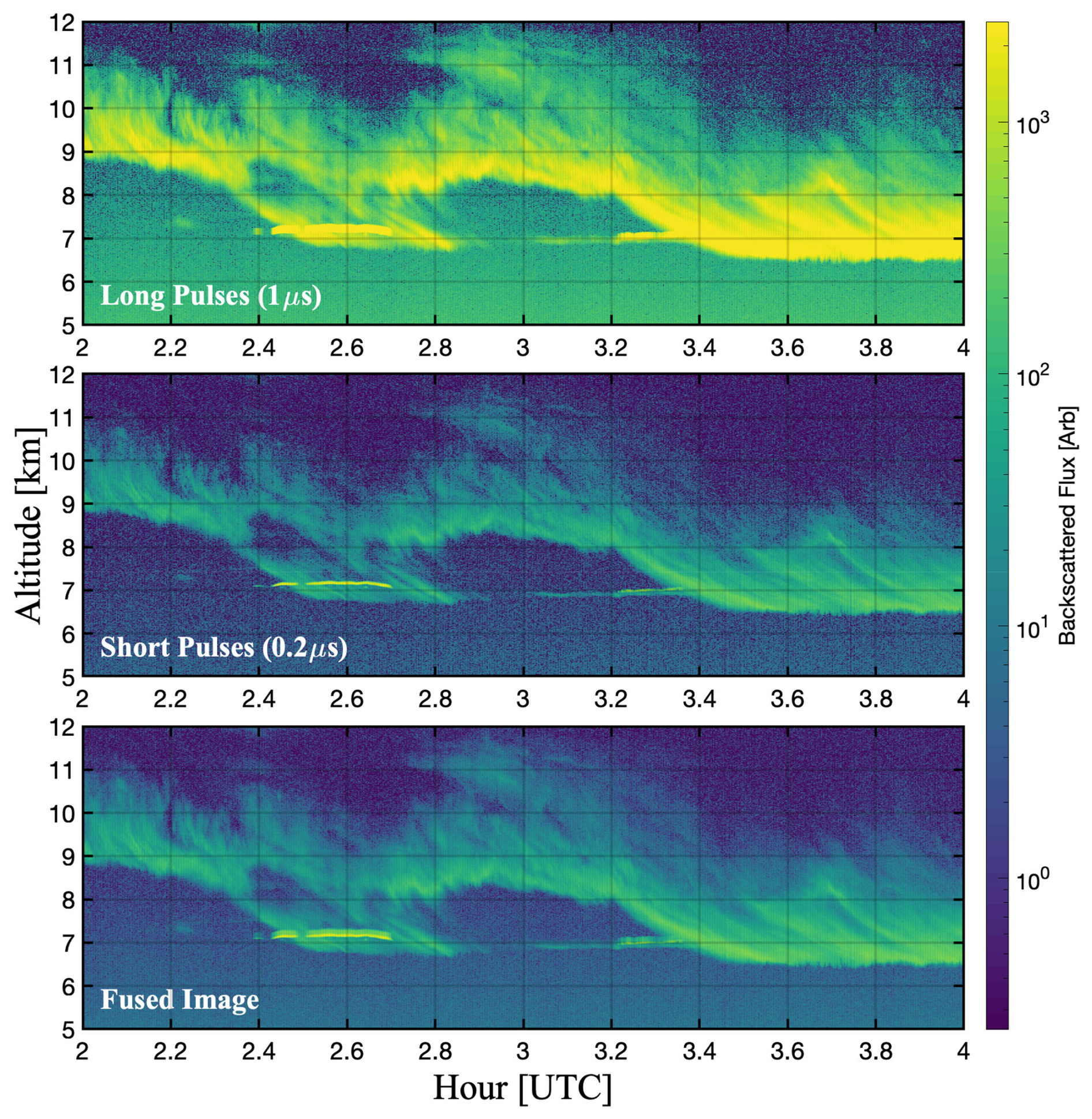
Figure 6 Cloud observations from 7 May 2024 in Albany, NY. Contours show observations of backscattered photon flux from the water vapor offline channel.

This particular cloud scene contains distinct varieties of cloud with different signal dynamic ranges. From approximately 2.4 to 2.7 UTC, at a range of approximately 7 km, there is a strong scattering target that is relatively thin. The layer vanishes at approximately 3.4 UTC. It is possible that this is a thin supercooled liquid containing cloud based on the relative signal strength. That thin liquid layer is embedded within less strongly scattering targets extending in range from approximately 6.75 to 12 km. These are likely ice clouds given their relative scattering efficiency and the layer's temperature (the layer has a temperature of approximately −20 °C at 7 km). For the sake of discussion, we will refer to these two cloud layers as liquid and ice for convenience of designation; it is practically irrelevant if this is correct. What is more relevant is that they have distinctly a different optical depth per meter and, by extension, produce disparate photon count rate dynamic ranges.

Examining the observation from the Long pulses, the ice clouds extend to at least 12 km; the same layer is not as clearly resolved when observed with Short pulses beyond 10.5 km. This is due to the higher overall power emitted from the Long pulses as compared to the Short pulses. In this case, the choice to use Short pulses causes errors in interpretation of the cloud scene; i.e., the observations are not completely representative of the atmosphere because they lack sensitivity. Considering that the tropopause tends to be lower at the poles and higher at the Equator (maybe 7 and 15 km above mean sea level, respectively), this could cause an observational bias of cloud occurrence and height.

In contrast to the observation of the ice clouds, the liquid cloud seems to have an oddly uniform thickness when observed with Long pulses. This is a result of the observations being a convolution of the scattering target and the laser pulse. In this case, the liquid cloud appears to be approximately 180 m thick when observed with a 1 µs pulse (150 m range smearing) and 60 m thick when observed with a 0.2 µs pulse (30 m range smearing). This indicates that the layer is likely not more than 30 m thick. The oddly uniform thickness when observed with the Long pulses is ostensibly an observation of the Long pulse itself. However, very thin cloud layers, such as those observed by McCullough et al. (2019), which were laminate structures on the order of 10 m thick, would be unobservable and effectively smeared together. The shorter the pulse, the more reasonable it would be to observe sharper features.

In this case, manual combination of the two layers would be challenging because they are not separated in space: one layer is embedded within the other. To combine this scene, and indeed many other cloud scenes in a general way, would require a method that was capable of balancing the sensitivity of each observation point by point. The previous example was simplified because we assumed the nature of this balance of sensitivity, i.e., that the Short pulses would be worse at observing to a greater range; that is untrue in this case and generally for cloud scenes. A body of literature exists on image fusion, which is designed to take two images of the same scene with different characteristics, for example, noise and resolution, and combine them (e.g., Patil and Mudengudi, 2011; Rani and Sharma, 2013; Li et al., 2017; Kaur et al., 2021; Trivedi and Sanghvi, 2023). A combined scene is presented based on principle component analysis in Fig. 6. This combined image does show some improvement in the ice clouds, where they appear more complete than those observed with Short pulses only, but the liquid cloud remains problematic. While it does appear thinner, the smearing from Long pulses persists. The scene could be merged, but it is not perfect; the scene inherits noise from Short pulses and smearing from Long pulses, albeit with lessened impact.

It is noteworthy that this image is somewhat different than a more canonical case described in the image fusion literature in that it is not high- and low-resolution per se. The resolution of the data acquiring Short and Long pulses are the same. The smearing of the features observed in Fig. 6 is happening because the pulse has a different width; therefore, there is a quasi-bias mechanism that will not be addressed directly. For the best performance, any image fusion scheme must be able to deconvolve the transmitted pulse characteristics and denoise the received signal to optimally represent the scene and effectively avoid inheriting the problematic parts of both observation methods². We are actively working on a forward model approach as a method of balancing these sensitivities in a general way.

6 Discussion and conclusion

The shot-to-shot alteration of pulse characteristics in this work has effectively provided the MPD instrument with a low-altitude observing channel. More traditional lidar systems have accomplished this in a number of ways, for example: (1) splitting the measured signal optically and analyzing it with two or more optical receivers, (2) altering the electrical gain of different observational circuits used for record detector voltages, or (3) splitting detector signals to do both analog detection and photon-counting detection simultaneously. It is worth noting that with a long pulse blinding the receiver, none of these other solutions are effective. The method introduced removes this issue but also has the advantage that it introduces no additional optical components and can work with purely photon-counting observations. The cost of this method is that the observational sensitivity comes from altering the lidar transmitter, not the receiver. Traditional techniques focused on the receiver serve to attenuate both the observed signal and the prime noise contribution, typically solar background and detector noise.

Given a single observational parameter (in this case, pulse width), maximum and minimum ranges have requirements that are essentially diametrically opposed. Historically, MPD has been run with pulse widths between 0.65 and 1 µs, with the vast majority being 1 µs. This has allowed for observation typically between 300 and 500 m and to approximately 4–6 km. This was found to be a reasonable compromise between competing desires to simultaneously see both as high and as low as possible. The timing unit demonstrated in this work has added a number of different parameters that can be used to better design the pulse strategy. The pulse width has been extensively discussed, but the duty cycle of pulses can be adjusted as well.

In this case, we have maintained Long pulses as the MPD standard 1 µs and simply shortened pulses in an attempt to see lower and at higher resolution. The 1 µs pulse was maintained because MPD performance in this mode is well understood and has been extensively validated. However, given that the compromise to see to lower altitudes was primarily what prevented the MPD pulse length from being longer originally, it is likely that longer pulses would increase the MPD maximum range with virtually no penalty, assuming it was paired with short pulses. Furthermore, we also used a 50/50 split among Long and Short pulses. This was chosen perforce by the MPD acquisition system requiring equal pulse numbers in its pre-integration. We are actively working to remove that limit. Assuming this hardware limitation is removed, it is also likely that a 50/50 split is not ideal. Given that the loss of received signal is a function of the range from the lidar system squared (R²), it is expected that a more skewed split (e.g., 90/10 or 95/5) would yield better long-range performance while not providing a major penalty for short-range observations.

The scope of this work has been to enhance the observational range of a diode-laser-based lidar system using shot-to-shot changes to pulse parameters. The solution proposed and demonstrated is a new timing system that has allowed for pulse-to-pulse changes in the laser shot duration. We have focused on a single parameter in an attempt to move the minimum range of observation to lower altitudes and to enhance the resolution of observations in clouds. In general, while it is beyond the scope of this work, we expect that extending the observational range will be further accomplished by skewing the pulse split towards longer pulses and allowing for longer pulses than 1 µs. An example might be a 90/10 Long/Short split with 2 and 0.2 µs lengths, respectively. This would focus most of the laser power and observations at the far range, where the signals are weakest, while simultaneously measuring low altitudes with adequate power to fill in observations at lower altitudes. It has not been our goal to optimize this design space but rather demonstrate, to our knowledge for the first time, a lidar-based observational system capable of this behavior. Furthermore, we plan future work to update the forward model of Marais and Hayman (2022) to include observations from multiple sensitivity observations to better leverage the information content of the two signals.

Appendix A

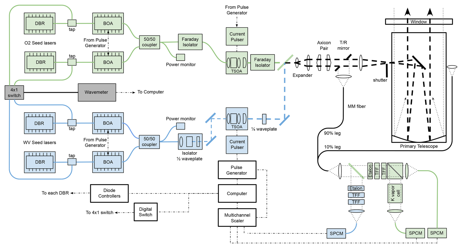
Figure A1 Block diagram of the MPD system. Blue components are for water vapor DIAL. Green components are needed for oxygen DIAL and potassium HSRL. Solid lines to the left of the TSOAs are polarization-maintaining single mode fibers. Dashed lines show the free space beam propagation. Acronyms: DBR – distributed Bragg reflector, BOA – booster optical amplifier, TSOA – tapered semiconductor optical amplifier, TFF – thin film filter, SPCM – single photon counting module, T/R – transmit/receiver, MM – multi-mode. The pulse generator shown is the master clock that has been altered for this work.