the Creative Commons Attribution 4.0 License.
the Creative Commons Attribution 4.0 License.
 | 05 Sep 2025
Harmonized cloud datasets for the Ozone Monitoring Instrument (OMI) and TROPOspheric Monitoring Instrument (TROPOMI) using the O2–O2 477 nm absorption band
Isabelle De Smedt
Nicolas Theys
Maarten Sneep
Pepijn Veefkind
Michel Van Roozendael
We present a new cloud retrieval algorithm using the O2–O2 absorption band at 477 nm, designed to provide harmonized cloud datasets from the Ozone Monitoring Instrument (OMI) and TROPOspheric Monitoring Instrument (TROPOMI). The goal of these derived cloud data is to mitigate the influence of clouds on the retrieval of tropospheric trace gases from UV–Visible nadir satellite spectrometers. The retrieval process consists of two main steps. First, spectral fitting is performed using the differential optical absorption spectroscopy (DOAS) method to determine the O2–O2 slant column and calculate the reflectance at the center of the fitting window. Second, these parameters are used to derive cloud fraction and cloud pressure.
This retrieval algorithm builds on the OMI O2–O2 operational cloud algorithm (OMCLDO2) with several improvements. The fitting procedure uses a broader fitting window, incorporating the O2–O2 absorption bands at 446 and 477 nm, to more accurately derive O2–O2 slant column densities (SCDs). A de-striping correction is applied to address across-track variability, and an offset correction of −0.08 × 1043 molec.2 cm−5, motivated by radiative transfer simulations, is applied in the TROPOMI retrieval to improve the consistency with OMI. Additionally, a temperature correction factor is included to account for the temperature dependence of both the O2–O2 SCD and the O2–O2 absorption cross-section. Consistent auxiliary data, such as meteorological information and a surface albedo database, are used for both sensors. Due to the inadequate signal-to-noise ratios in the daily solar irradiance measurements by OMI, a fixed annual-averaged irradiance for 2005 is used as a reference for the reflectance spectra in the spectral fittings.
To evaluate the performance of our retrieval approach, we compare it with the OMCLDO2 algorithm for both OMI and TROPOMI. The cloud fraction retrievals demonstrate good agreement, whereas the cloud pressure retrievals show a systematic bias, particularly in nearly cloud-free scenes. Our cloud pressure estimates tend to be higher than OMCLDO2 for OMI and lower for TROPOMI. Notably, our approach demonstrates improved consistency in cloud parameters, especially cloud pressure, between the two sensors compared to OMCLDO2. However, a consistent bias of approximately 0.05 in cloud fraction retrievals is observed, primarily attributed to differences in L1b data that show systematic biases between the OMI and TROPOMI reflectances. Applying these cloud corrections to NO2 retrievals reveals that the average impact of cloud corrections ranges from −6 % to 11 % in polluted regions. Differences in NO2 air mass factor (AMF) resulting from varying cloud correction methods can exceed 10 %. Importantly, the new correction approach achieves better consistency in NO2 retrievals between OMI and TROPOMI.
- Article
(12802 KB) - Full-text XML
- BibTeX
- EndNote


Clouds play a crucial role in Earth's climate system and hydrological cycle by reflecting shortwave solar radiation and absorbing and re-emitting longwave radiation from Earth. Satellite UV–Visible sensors, such as the Ozone Monitoring Instrument (OMI) and TROPOspheric Monitoring Instrument (TROPOMI), designed for trace gas measurements, have relatively coarse spatial resolutions – ranging from several to hundreds of kilometers. Consequently, only a small fraction (5 %–20 %) of observed pixels are cloud-free, while most are partially covered by cloud (Krijger et al., 2007). Clouds significantly impact the accuracy of trace gas retrievals, making it essential to account for their effects.
Due to the complexity of cloud effects on the atmospheric radiation field, trace gas retrievals often rely on several simplifying assumptions. The key assumptions are (1) the independent pixel approximation (IPA; Martin et al., 2002; Boersma et al., 2004; Stammes et al., 2008), which neglects horizontal radiative energy transport between clear and cloudy subpixels, and (2) the assumption that clouds are horizontally and vertically homogeneous, thereby simplifying radiative transfer processes within clouds. Accurate estimation of photon path lengths in the atmosphere is crucial for precise trace gas retrievals, as these paths determine trace gas absorption and influence the measured top-of-atmosphere (TOA) radiance. Under cloudy conditions, photon path lengths are primarily influenced by the cloud's geometric fraction and vertical extinction profile (Stammes et al., 2008).
The Dutch–Finnish-built OMI, a key payload aboard the NASA Aura spacecraft, is a nadir-viewing, wide-swath, push-broom imaging spectrometer designed for daily global monitoring of tropospheric composition. OMI provides two operational cloud products, both based on determining the mean photon path in the UV–Visible spectrum by analyzing the spectral features of species with a known vertical distribution but using different physical processes. The OMCLDO2 cloud product (Acarreta et al., 2004; Sneep et al., 2008; Veefkind et al., 2016) uses satellite measurements of the O2–O2 collision complex absorption feature centered at 477 nm. In contrast, the OMCLDRR cloud product (Vasilkov et al., 2004; Joiner and Vasilkov, 2006; Vasilkov et al., 2008) is based on the filling-in of Fraunhofer lines in the UV, caused by rotational Raman scattering (RRS) by air molecules, and it uses a spectral window of 345–354 nm. Both algorithms use the IPA, which characterizes pixel reflectance as a weighted combination of cloudy and clear-sky parts. This approach enables the determination of the effective cloud fraction rather than the geometric cloud fraction. Due to limited spectral information in the O2–O2 absorption band and the RRS process that are used for cloud pressure retrieval, the cloud is modeled as a Lambertian reflector with a fixed albedo of 0.8. Consequently, only the altitude level of this Lambertian cloud is retrieved.
TROPOMI, aboard the Sentinel-5P platform, is the first Copernicus mission dedicated to atmospheric monitoring, providing daily city-scale measurements for air quality assessment, ozone and UV radiation monitoring, and climate observation and forecasting. Several cloud products have been developed for TROPOMI using different methodologies to measure cloud parameters such as fraction, height (or pressure), and optical thickness. The operational cloud product includes the Optical Cloud Recognition Algorithm (OCRA) and the Retrieval Of Cloud Information using Neural Networks (ROCINN), which work together to retrieve cloud properties. OCRA determines cloud fraction by analyzing the broadband color of the measured spectra, while ROCINN uses the O2 absorption band (756–771 nm) to estimate cloud-top height and cloud optical thickness (or cloud-top albedo). Additionally, the Fast Retrieval Scheme for Clouds from the Oxygen A band (FRESCO) algorithm utilizes three reflectance bands around the O2–A band (Koelemeijer et al., 2001; Wang et al., 2008) to estimate cloud pressure and cloud fraction from TOA reflectances. The TROPOMI implementation, known as FRESCO-S, introduces several improvements over the FRESCO+ algorithm originally developed for GOME-2 (van Geffen et al., 2022, 2024). In the latest update (processor version 2.8.0), the algorithm switched to a two-band retrieval approach, excluding the strongest absorption band (760–761 nm). This change was implemented to eliminate biases in cloud height retrievals that erroneously position clouds closer to the surface or even below it (van Geffen et al., 2024). The cloud model assumptions remain consistent with those employed in the OMCLDO2 and OMCLDRR algorithms. Since processor version 2.2 (van Geffen et al., 2022), the O2–O2 cloud product has been integrated into the NO2 processing chain, leveraging a similar O2–O2 cloud retrieval algorithm as previously used by OMI.
Latsch et al. (2022) present a comprehensive intercomparison of various TROPOMI cloud products, revealing significant differences among algorithms, particularly under conditions of small cloud fractions and low cloud heights – critical scenarios for accurate tropospheric trace gas retrievals. Bauwens et al. (2020) identified a systematic discrepancy in NO2 retrievals between the OMI QA4ECV product and the TROPOMI operational product, primarily due to differences in the cloud products used. These differences are significantly reduced following the update of the cloud retrieval (van Geffen et al., 2022). Similarly, De Smedt et al. (2021) discovered that variations in cloud products contribute to biases in HCHO retrievals between OMI and TROPOMI. Furthermore, even when applying the same algorithm to different sensors, systematic differences can appear in the results.
In this paper, we present a new cloud retrieval algorithm using the O2–O2 absorption band at 477 nm, designed to provide harmonized cloud datasets from OMI and TROPOMI. The retrieval algorithm builds on the operational OMI cloud product (OMCLDO2), incorporating several key improvements. To optimize the differential optical absorption spectroscopy (DOAS) fitting, we extend the spectral range and implement an additional de-striping correction to reduce variability between tracks in the O2–O2 slant column density (SCD) retrievals. We ensure consistency between the O2–O2 SCD measurements from OMI and TROPOMI through comparative analysis. Additionally, we introduce an improved temperature correction factor to account for the temperature dependence of the O2–O2 absorption cross-section in the conversion from O2–O2 SCD and TOA reflectance to cloud parameters. Furthermore, the TROPOMI directionally dependent Lambertian-equivalent reflectivity (DLER) climatology dataset is employed in the retrievals for both sensors.
The structure of this paper is as follows. We start with an introduction of the instruments and the latest version of the Level-1b (ir)radiance spectra used in this study (Sect. 2). Next, we outline the key aspects and implementation of the new BIRA-IASB O2–O2 cloud algorithm (Sect. 3). We then compare the BIRA-IASB retrievals with the OMI and TROPOMI OMCLDO2 products (Sect. 4.1) and assess their application to tropospheric NO2 retrieval, focusing on the impact of clouds on trace gas retrievals (Sect. 4.2). Additionally, we present comparisons of cloud products and NO2 retrieval using these cloud corrections for OMI and TROPOMI (Sect. 4.3). The paper concludes with a summary of our findings in Sect. 5.
2.1 OMI and TROPOMI
OMI, a nadir-viewing imaging spectrograph developed by the Netherlands and Finland, was launched in 2004 aboard NASA's Earth Observing System (EOS) Aura satellite (Levelt et al., 2006). Operating in an ascending Sun-synchronous polar orbit, OMI crosses the Equator at approximately 13:40 LT (local time). It measures solar radiation backscattered by the Earth's atmosphere and surface, covering a wavelength range of 270–500 nm with a spectral resolution of roughly 0.5 nm. With a 114° viewing angle, OMI provides a 2600 km swath width, enabling daily global coverage. The individual ground pixels measure 13 km (along-track) by 24 km (across-track) at the center of the swath, increasing to about 150 km towards the edges. The swath is divided into 60 across-track ground pixels, with incoming light depolarized by a scrambler and split into three spectral channels: two UV channels (UV1 and UV2, covering 270–380 nm) and one visible channel (350–500 nm).
TROPOMI, aboard the Copernicus Sentinel-5 Precursor (S5P) satellite (Veefkind et al., 2012), is a four-channel, nadir-viewing grating spectrometer that measures solar backscattered radiances across the UV, visible, near-infrared (NIR), and shortwave infrared (SWIR) spectra. Like OMI, TROPOMI operates from an ascending Sun-synchronous polar orbit, crossing the Equator at about 13:30 LT. It retains comparable spectral resolution and radiometric performance in the ultraviolet and visible ranges but offers enhanced spatial resolution. At the center of the swath, the ground pixels measure 7 km along-track (reduced to 5.6 km as of 6 August 2019) and vary from 3.5 to 25 km across-track, depending on the wavelength band. With a 2600 km swath width, TROPOMI achieves near-global daily coverage, excluding narrow strips approximately 0.5° wide between orbits at the Equator. The swath is divided into 77 to 450 rows, with the binning factor adjusted to ensure similar spatial size for each row, The exact number of rows depends on the spectral band.
2.2 OMI Level-1b irradiance and radiance spectra
The BIRA-IASB O2–O2 cloud product for OMI utilizes the OML1BIRR and OML1BRVG product from the OMI Collection 4 dataset (processor version: 2.0.8.4/24861), which is publicly accessible through NASA's Goddard Earth Sciences Data and Information Services Center (GES DISC). This dataset employs a newly developed L0-1b processor, based on the TROPOMI L0-1b processor at the OMI Science Investigator-led Processing System (OMI SIPS). The advanced processor converts raw sensor data into radiometrically calibrated and geolocated solar irradiances and earthshine radiances. Building on 17 years of experience with OMI Collection 3 data, significant improvements have been made to address issues related to optical and electronic aging and to enhance pixel quality flagging. Detailed information about the upgrade from Collection 3 to Collection 4 is provided in Kleipool et al. (2022). The OML1BIRR contains daily-averaged irradiance measurements, while the OML1BRVG product contains Earth-view spectral radiances recorded in global mode from the visible detector.
Since 2007, OMI has experienced a field-of-view blockage known as the “row anomaly”, which affects data quality across all retrieval wavelengths for certain rows (Dobber et al., 2008). The row anomaly has been analyzed for the entire mission for the UV2 and VIS channels, determining affected rows for each day at two wavelengths per channel. Based on these analyses, a dynamic map is generated and used by the Collection 4 L0-1b processor to flag rows accordingly over time. The row anomaly initially affected two rows in June 2007 but eventually extended to approximately 50 % of the sensor's 60 rows. Moreover, the row anomaly is not static and evolves slowly over both long and short timescales.
2.3 TROPOMI Level-1b irradiance and radiance spectra
The initial version of the TROPOMI L1b spectra, based on pre-launch calibration, is described in detail by Kleipool et al. (2018), while subsequent improvements informed by in-flight calibration are comprehensively documented in Ludewig et al. (2020). This study uses the updated version of the L1b (ir)radiance dataset (processor version: 2.1.0.25042), which has been reprocessed since 2022.
TROPOMI measurements can experience saturation in band 4 (visible) and band 6 (NIR) detectors when observing intensely bright scenes, such as high clouds in tropical regions. This saturation can affect the O2–O2 cloud retrievals, which rely on measurements from band 4. To mitigate this, spectral pixels flagged as saturated are excluded from data analysis. Saturation can lead to anomalously low radiances for certain spectral pixels. Significant saturation can also cause “blooming”, where excess charge from saturated pixels spills into adjacent ground pixels along the row direction, leading to anomalously high radiances for some spectral pixels. Both saturation and blooming are identified and flagged under a single error flag, as documented by Ludewig et al. (2020). The revised irradiance product includes corrections for optical degradation, improvements in absolute irradiance calibration, and adjustments for the solar radiation angle dependence of the irradiance signal. Additionally, degradation correction is applied to the radiance data.
3.1 Heritage
The O2–O2 cloud algorithm, developed by KNMI and known as OMCLDO2, was specifically designed for OMI measurements, as OMI does not cover the spectral range of the O2 A-band at 760 nm (Acarreta et al., 2004; Sneep et al., 2008; Veefkind et al., 2016). This algorithm utilizes satellite measurements of O2–O2 collision complex absorption near 477 nm to retrieve essential cloud parameters. The procedure involves two main steps. First, a DOAS fit is applied to determine the O2–O2 slant column amount, with reflectance calculated at the center of the fitting window. Second, these parameters are converted into effective cloud fraction and effective cloud pressure using a Lambertian cloud model, which assumes that clouds act as Lambertian reflectors with a fixed albedo of 0.8 (Stammes et al., 2008). This cloud product is designed to mitigate cloud effects in trace gas retrievals, and the cloud model assumptions are consistent across both cloud and NO2 retrievals. Validation indicates that the retrieved cloud pressure corresponds to the mid-level of the cloud rather than the cloud-top pressure (Sneep et al., 2008). It is important to note that this algorithm does not distinguish between clouds and aerosols. Consequently, in the computation of the air mass factor (AMF) for trace gas retrieval, aerosol-induced cloud parameters can implicitly correct part of the aerosol effects (Boersma et al., 2011).
The OMCLDO2 algorithm was first described by Acarreta et al. (2004), and Veefkind et al. (2016) further improved the retrieval approach. The improvements primarily involve correcting differences in the temperature profile and consequently in the absorption coefficient due to density changes between the GEOS-5 Forward Processing for Instrument Teams (FP-IT) model profile and the fixed model profile used in the forward calculations. Additionally, the look-up table (LUT), which is pre-inverted, has also been updated. The OMI OMCLDO2 product used in this study is based on the most recent version of the OMI L1b dataset (Collection 4 data; Kleipool et al., 2022). Since the release of the TROPOMI operational NO2 processor version 2.2, the O2–O2 cloud product has been included in the NO2 data product files (van Geffen et al., 2022). However, it has not yet been utilized in trace gas retrievals.
The BIRA-IASB O2–O2 cloud retrieval algorithm, though similar in many aspects to OMCLDO2, incorporates several enhancements to improve accuracy and consistency across different sensors:
-
The DOAS slant column fitting employs a larger fitting window, capturing two O2–O2 absorption bands at 446 and 477 nm.
-
A de-striping correction is applied to reduce across-track variability.
-
An SCD offset correction is implemented to ensure consistency between OMI and TROPOMI measurements.
-
A temperature correction addresses the temperature dependence of the O2–O2 cross-section.
-
Consistent auxiliary data, such as meteorological information and surface albedo database, are utilized for both OMI and TROPOMI sensors.
The following section details the BIRA-IASB O2–O2 cloud retrieval approach, with an emphasis on these improvements relative to the OMCLDO2 algorithm.
3.2 DOAS slant column retrieval
Table 1 summarizes the absorption cross-sections and settings used for retrieving O2–O2 slant columns. Several improvements have been made to the DOAS fitting compared to the OMCLDO2 algorithm. While OMCLDO2 performs the DOAS fit over a spectral range of 460–490 nm, accounting for the absorption effects of NO2, O3, and O2–O2, the BIRA-IASB approach employs a wider fitting window of 435–495 nm. This expanded range includes both a strong absorption band centered at 477 nm and a weaker absorption band around 447 nm. The wider fitting range improves the stability of the retrieval by reducing the sensitivity of O2–O2 SCD retrievals to the polynomial order chosen in the DOAS settings. The inclusion of this broader range necessitates additional spectral analysis adjustments. For example, the fitting now incorporates gas species like water vapor, along with a liquid water absorption cross-section (Peters et al., 2014), to mitigate systematic errors over oceans. Importantly, this revised DOAS approach aligns closely with NO2 DOAS retrievals (405–465 nm, Boersma et al., 2007; van Geffen et al., 2022), owing to the substantial overlap between the O2–O2 and NO2 fitting windows.
Thalman and Volkamer (2013)Vandaele et al. (2002)Serdyuchenko et al. (2014)Gordon et al. (2022)Pope and Fry (1997)(Chance and Spurr, 1997)Table 1Summary of absorption cross-sections and settings used for the retrieval of O2–O2 slant columns.
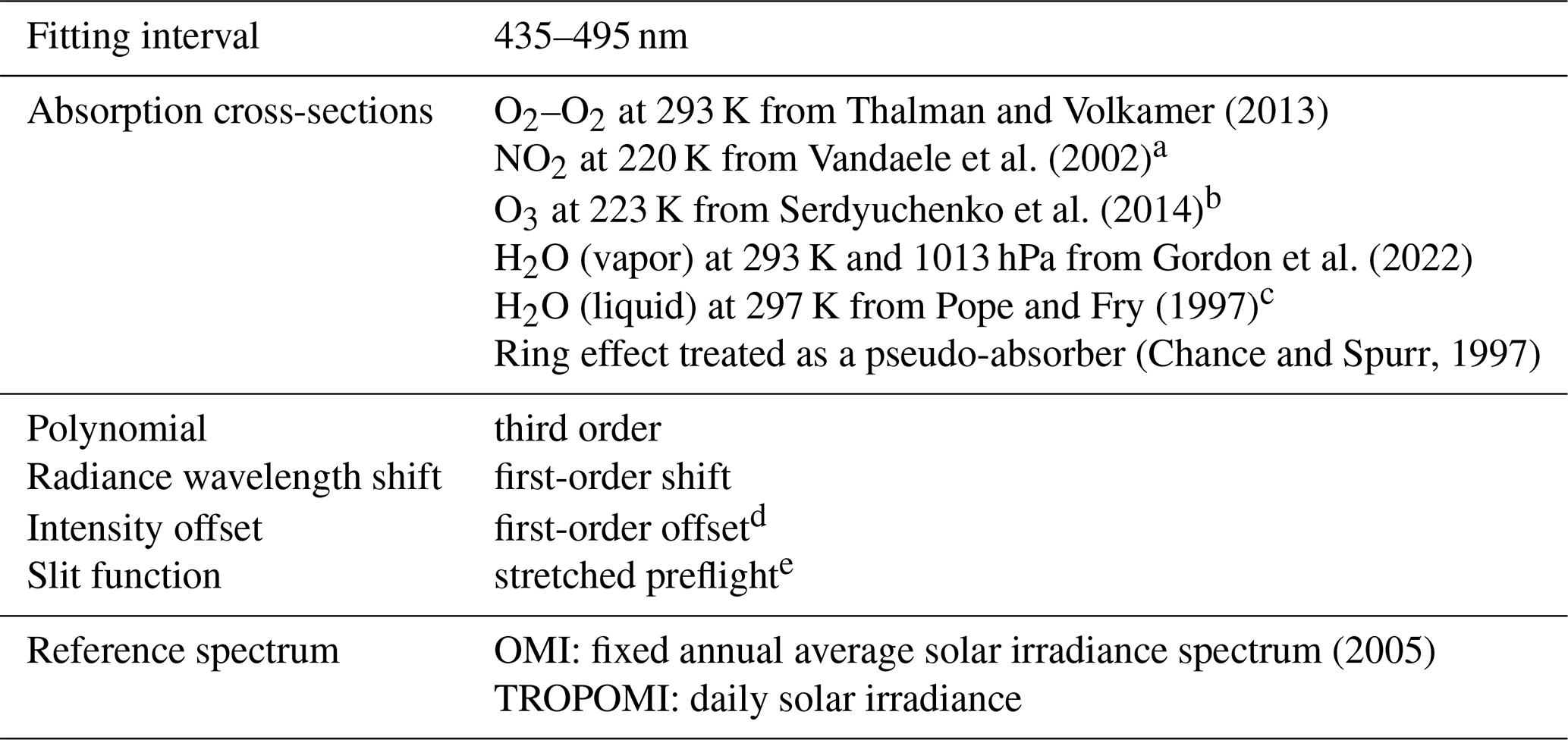
The a I0 correction is applied based on a NO2 SCD of 5 × 10¹⁵ molec. cm−2 using Eq. (A3) from Aliwell et al. (2002). The b I0 correction is applied based on a O3 SCD of 2 × 10¹⁹ molec. cm−2 using Eq. (A3) from Aliwell et al. (2002). c Smoothed as in Peters et al. (2014). d Additional cross-section taken as the inverse of the reference spectrum (see Eq. 5.6 in Danckaert et al., 2017). e Stretch factors as fit parameters to adjust instrument slit function width.
The latest available cross-sections for species absorbing within the selected fitting window are utilized in the analysis. The absorption cross-sections of the oxygen dimer, which are crucial for this analysis, are depicted in Fig. 1. It should be noted that there is a systematic 3 % difference in the O2–O2 slant columns between the retrieval using the O2–O2 cross-sections from Thalman and Volkamer (2013) and Finkenzeller and Volkamer (2022). The fitting residuals using these two O2–O2 cross-sections are generally similar; however, the latter exhibits larger residuals in cases influenced by liquid water. Additionally, the dataset from Thalman and Volkamer (2013) includes cross-sections at a greater number of temperatures, allowing for a more detailed investigation of temperature dependence. In the slant column density fit, an absorption cross-section with a fixed temperature is used. Changing the temperature of O2–O2 cross-section from 293 to 253 K results in a reduction of approximately 4 % in the retrieved O2–O2 slant columns. This temperature dependence is subsequently corrected in the calculations using a similar approach to the one described in Boersma et al. (2004), which will be discussed in Sect. 3.5.3.
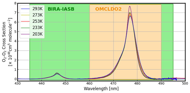
Figure 1Temperature-dependent absorption cross-sections of O2–O2 collision pairs between 430 and 500 nm from Thalman and Volkamer (2013). The fitting window used for the OMCLDO2 retrieval is shown in orange, while the larger range used in this study is indicated in green.
Intensity offsets in the spectra, caused by factors such as residual stray light, are corrected by fitting the inverse of the solar reference spectrum (see Eq. 5.6 of Danckaert et al., 2017). In addition, the DOAS fit procedure includes a spike removal scheme as described in Richter et al. (2011), which allows us to filter out individual corrupted radiance measurements from the fit and hence reduce the noise in the retrieval. This approach is also included in the OMCLDO2 algorithm (Veefkind et al., 2016). In this study, the slant columns are derived using the QDOAS software developed at BIRA-IASB (Danckaert et al., 2017).
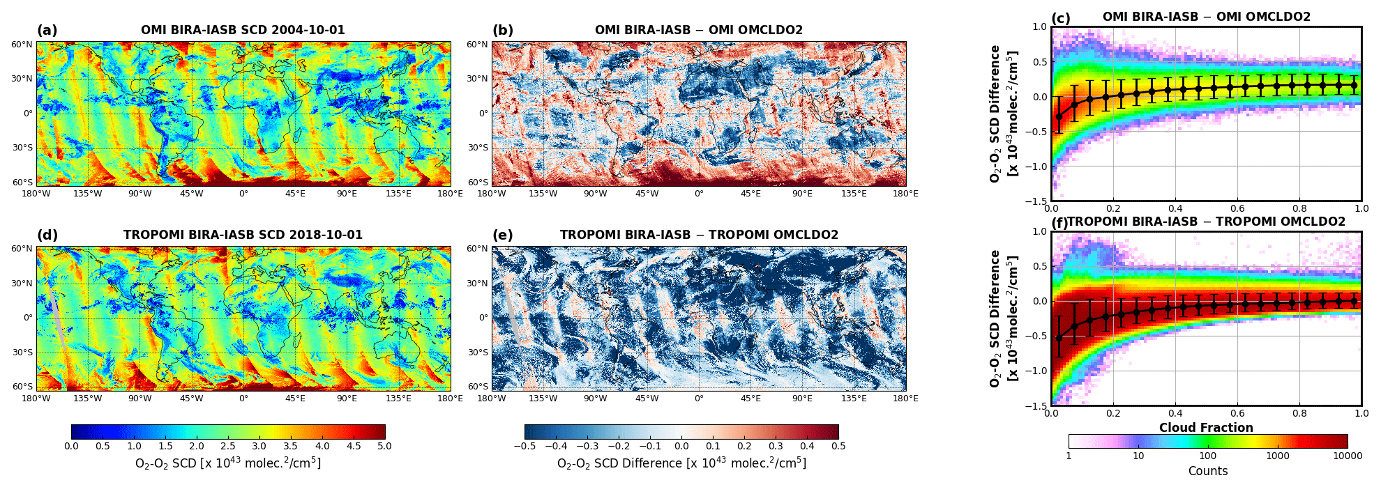
Figure 2A comparison of O2–O2 SCD retrievals between BIRA-IASB and OMCLDO2 is shown for the OMI measurement on 1 October 2004 (a–c) and for the TROPOMI measurement on 1 October 2018 (d–f). Panels (a) and (d) present the BIRA-IASB O2–O2 SCD retrievals, while panels (b) and (e) show the SCD differences between the BIRA-IASB and OMCLDO2 algorithms. Panels (c) and (f) depict the SCD difference as a function of BIRA-IASB cloud fraction for snow- and/or ice-free pixels between 50° S and 50° N latitude. The black circles with error bars represent the binned average values, including their standard deviations, and the color bar indicates sample counts.
Figure 2 presents O2–O2 retrievals based on the BIRA-IASB approach and a comparison with OMCLDO2. The data shown are based on OMI measurements on 1 October 2004 and TROPOMI measurements on 1 October 2018. The OMI OMCLDO2 data use the Product Generation Executive (PGE) version 4.0.0.308, based on the OMI Collection 4 L1 dataset, while the TROPOMI OMCLDO2 data come from the operational NO2 product processor version 2.2, based on TROPOMI Collection 3 Level 1 data. Although the observations are from different times, a comparison of Fig. 2a and d shows that TROPOMI SCDs are slightly higher than OMI SCDs for low SCD values. For OMI, the differences between BIRA-IASB and OMCLDO2 algorithms indicate a relatively large negative bias over land and a positive bias at high latitudes. For TROPOMI, the biases are predominantly negative, particularly over land regions. The across-track dependence visible in the OMI difference map is likely caused by calibration issues in the OMI L1b data, which introduce across-track variability in trace gas retrievals (Boersma et al., 2007), and this effect varies depending on the retrieval approach used. A correction methodology for this effect will be detailed in the following section. The dependence on cloud fraction, as shown in Fig. 2c and f, indicates that the significant biases are primarily associated with cases for small cloud fraction.
The TOA reflectance is calculated at the central wavelength of the fitting window (465 nm) with a bandwidth of 1 nm. For TROPOMI, the solar irradiance reference is derived from daily solar irradiance measurements. In contrast, for OMI, the limited quality of the daily solar measurements necessitates using a 100 d running mean of solar irradiance data, further smoothed to enhance accuracy (Ludewig et al., 2020). However, this approach still does not satisfy the precision requirement of the DOAS fitting. Consequently, a fixed annual average irradiance spectrum from 2005 is applied.
3.3 Correction for across-track variability
OMI data reveal systematic biases in retrievals, appearing as a striped pattern across cross-track positions – an issue commonly observed in satellite sensors equipped with 2-D detector arrays (Boersma et al., 2011). To mitigate this artifact, a “de-striping” correction can be applied (Boersma et al., 2007, 2011). Alternatively, the reference sector method offers another approach to mitigate this issue (De Smedt et al., 2015).
To evaluate the across-track variability of O2–O2 slant column retrievals for OMI and TROPOMI, we analyze data collected between 50° S and 50° N, focusing specifically on ocean pixels. For each row, 7 d median O2–O2 SCD values are computed and plotted as a function of the tangent of the viewing zenith angle (tan (θ)), as shown in Fig. 3a. Negative viewing zenith angle (VZA) values correspond to satellite measurements on the west side of the swath. OMI results are analyzed across multiple years to explore interannual variability over the same time period. The results reveal that TROPOMI SCDs display significantly smoother across-track variability compared to OMI, consistent with findings from previous NO2 retrieval studies (van Geffen et al., 2020).
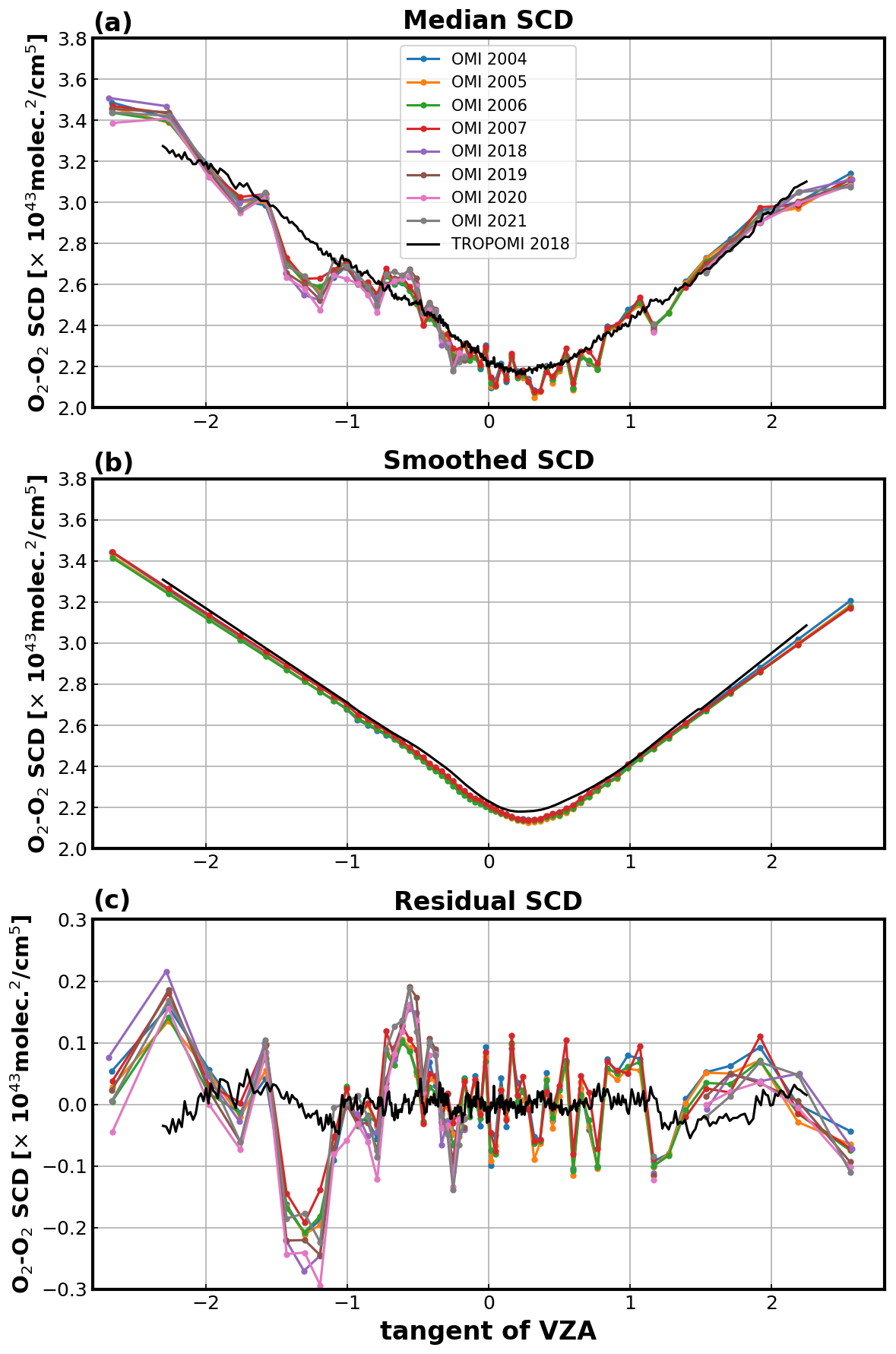
Figure 3Row dependence of O2–O2 SCD from OMI and TROPOMI over ocean. (a) Median values between 50° S and 50° N for 1–7 October of the selected years, presented as a function of the tangent of VZA (tan (θ)), with negative values indicating measurements from the west-viewing direction. Note that OMI measurements for 2018–2021 between rows 22 and 54 (0-based) are excluded from the analysis due to the row anomaly; (b) smoothed SCD values computed using the method described in Sect. 3.3; and (c) residual SCD, calculated as the difference between median and smoothed values. For OMI, the residual SCDs for 2018–2021 are calculated based on the average of smoothed SCDs from 2004 to 2007.
Compared to trace gas retrievals, identifying suitable reference data for correcting stripe patterns in O2–O2 is more challenging. In this work, we present a “de-striping” approach to eliminate across-track biases in O2–O2 SCDs for OMI measurement across different viewing angles:
-
We compute the median O2–O2 SCD for each row over ocean pixels using 7 consecutive days of measurements between 50° S and 50° N. These median values are plotted as a function of tan (θ).
-
We apply a linear fit to data at the swath edges ( or tan (θ) > 0.5), and we use a Savitzky–Golay filter for the measurements near nadir (). Finally, we average the smoothed SCDs over the period 2004–2007.
-
We collect the median SCDs obtained from step 1 for rows 2 to 21, calculate their average, and then compare this value with the mean of similarly calculated values from the same period during the reference years (2004–2007) to determine an offset, which reflects the interannual variation of O2–O2 SCD in the selected region.
-
We calculate the stripe amplitude by subtracting the offset and the 4-year-averaged smoothed SCDs for all across-track rows.
The O2–O2 SCD is highly sensitive to variations in both along-track and across-track solar and viewing zenith angles, as well as to surface albedo, surface pressure, and cloud parameters. The data selection method used in Fig. 3a excludes land regions due to the significant spatial and temporal variations in surface albedo and surface pressure, as these factors strongly affect the O2–O2 SCD. Additionally, using median values helps mitigate the effects of clouds on the O2–O2 SCDs, allowing the observed variations to be primarily attributed to geometric factors, particularly viewing zenith angles. As shown in Fig. 3a, TROPOMI SCDs exhibit an almost linear dependence on tan (θ) for both the west and east sides of the swath. Therefore, we propose using the described method to smooth the O2–O2 SCD.
After 2007, an anomaly began affecting OMI radiances in certain cross-track positions, making the second step of the smoothing process inapplicable. However, Fig. 3b demonstrates that the smoothed SCDs exhibit minimal interannual variation. This finding has been further confirmed for other periods, indicating interannual differences of up to 0.1 × 1043 molec.2 cm−5 (not shown). Thus, we use the average from 2004 to 2007 as a reference. Additionally, an offset is calculated based on the measurements from rows 2–21 (0-based), which remain unaffected by the anomaly throughout all periods, and this offset correction is applied to further mitigate small interannual variations.
Figure 3c illustrates the across-track variability corrections for 1–7 October for selected years for both OMI and TROPOMI. The correction for TROPOMI follows the same methodology as described above, using the 2018 average as a reference. The OMI amplitudes reach up to 0.3 × 1043 molec.2 cm−5, with a slight increase observed over time, whereas the TROPOMI amplitudes are much lower, remaining below 0.05 × 1043 molec.2 cm−5. The typical precision of O2–O2 SCD from DOAS fits is approximately 0.07 × 1043 to 0.1 × 1043 molec.2 cm−5 for OMI in 2004 and 2018, which is lower than the observed amplitude variations. In contrast, for TROPOMI, the O2–O2 precision is around 0.05 × 1043 molec.2 cm−5, making it comparable to the amplitude variations. As a result, this correction is currently applied only to OMI data.
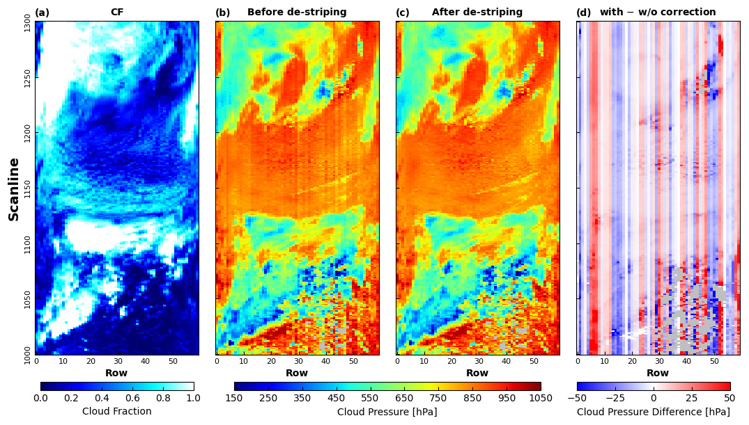
Figure 4OMI O2–O2 cloud retrievals for BIRA-IASB cloud fraction (a), BIRA-IASB cloud pressure before (b) and after (c) de-striping correction, and (d) difference between with and without correction. The data shown represent a segment of an OMI swath (scan lines 1000–1300) from orbit 1132 on 1 October 2004. Pixels with cloud fractions below 0.05 have been removed from the cloud pressure maps.
As illustrated in Fig. 4, a stripe pattern is visible in the cloud pressure retrievals, particularly over nearly cloud-free scenes. The de-striping correction effectively reduces cloud pressure variability across the track. As shown in Fig. 4d, the differences in cloud pressure due to this correction are generally within ±30 hPa, with significantly larger deviations observed when the cloud fraction approaches zero. Additionally, this impact on cloud fraction retrieval is negligible (not shown).
3.4 Offset correction for slant column density
To further validate the O2–O2 SCD retrieval, we compared the measured O2–O2 SCDs with those simulated using a radiative transfer model. For ground-based measurements, a scaling factor is often required to align measured and modeled O2–O2 absorptions (Wagner et al., 2009; Clémer et al., 2010). Wagner et al. (2019) assess various sources of uncertainty in both measurements and simulations, emphasizing the importance of accurately characterizing the atmospheric state, measurement conditions, and spectral analysis to minimize discrepancies.
To accurately simulate O2–O2 absorption, we adopt the method described in Eq. (8) of Veefkind et al. (2016) with an improvement to calculate the O2–O2 slant column under clear-sky conditions, as follows:
where Rg is the gas constant, M is the mean molecular mass of dry air, g is the gravity acceleration, kB is Boltzmann's constant, and m represents the clear-sky box-AMF calculated at 465 nm. The mixing ratio of oxygen is assumed to be 20.9476 %. Compared to Eq. (8) of Veefkind et al. (2016), a correction factor c is included to account for the temperature effect on the O2–O2 cross-section. Since the O2–O2 SCD retrieval uses an absorption cross-section at a fixed temperature, this factor aligns the retrieved and modeled O2–O2 absorption, compensating for the variation of O2–O2 absorption due to temperature changes. Details on the calculation of the correction factor c will be discussed in Sect. 3.5.3. For temperature profiles, we use the CAMS reanalysis data – the latest global atmospheric composition reanalysis produced by the Copernicus Atmosphere Monitoring Service (CAMS). The data are provided at 3 h intervals and include 60 vertical hybrid sigma–pressure levels, with the top level at 0.1 hPa. Additionally, surface reflectance is obtained from the TROPOMI monthly DLER database (Tilstra et al., 2024), which is used for the AMF calculations.
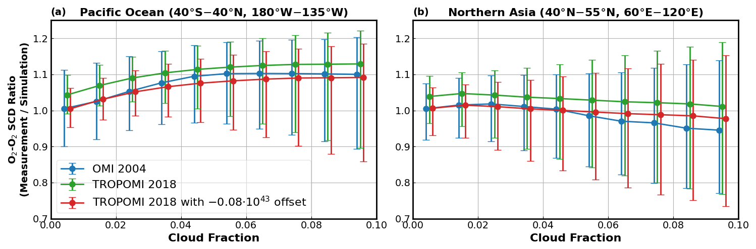
Figure 5Ratio of measured to retrieved O2–O2 SCD to simulated clear-sky O2–O2 SCD as a function of cloud fraction for two remote regions: (a) Pacific Ocean and (b) northern Asia. The analysis is based on 1 month of OMI measurements from October 2004 and TROPOMI from October 2018, considering only pixels with a VZA of below 60°. Data are binned by cloud fraction intervals of 0.01, showing the 10th percentile (lower error bar), median (circle), and 90th percentile values of the ratio. Additionally, the figure includes the ratio for TROPOMI O2–O2 SCD with an offset of −0.08 × 1043 molec.2 cm−5 (see Sect. 3.4 for further discussion).
Figure 5 shows the ratio of retrieved O2–O2 SCD to simulated clear-sky O2–O2 SCD as a function of cloud fraction over two remote regions, where aerosol effects can be neglected. The analysis is based on 1 month of OMI measurements from October 2004 and TROPOMI from October 2018, considering only pixels with a VZA below 60°, For OMI data, the de-striping correction is applied. The results indicate that the OMI ratios approach 1 when the cloud fractions are near zero, consistent with our expectations. Additionally, as the cloud fraction increases, median ratio values rise over the ocean and fall over land, suggesting that low clouds are more prevalent over ocean, while high clouds are more frequent over land, consistent with previous findings (Tan et al., 2023). TROPOMI ratios are systematically higher than those of OMI. When an offset of −0.08 × 1043 molec.2 cm−5 is applied to the TROPOMI SCDs, the ratios align more closely with OMI results. This offset reflects the difference in the mean O2–O2 SCD values between OMI and TROPOMI for scenes with cloud fractions between 0 and 0.05 in the two study regions. Further tests, such as restricting pixels to nadir measurements (θ<30°), adjusting spectral fitting settings, and analyzing data from other time periods, yielded similar conclusions (not shown). Although factors like surface reflectance precision and aerosol effects may influence the O2–O2 simulation and although DOAS settings may affect the accuracy of the O2–O2 SCD retrieval, the bias between OMI and TROPOMI remains unchanged. A potential explanation for this discrepancy is the difference in the solar reference spectrum. While further investigation is needed, it lies beyond the scope of this study. To ensure consistency between OMI and TROPOMI in this study, an offset of −0.08 × 1043 molec.2 cm−5 is applied to the TROPOMI data. This adjustment leads to a cloud pressure retrieval approximately 50 hPa higher in nearly cloud-free scenes, with the effect diminishing as the cloud fraction increases.
3.5 Conversion to cloud parameters
3.5.1 Radiative transfer simulation
To convert the DOAS fit parameters into cloud fraction and cloud pressure, we use version 2.8 of the Vector-LInearized Discrete Ordinate Radiative Transfer (VLIDORT) radiative transfer model (RTM) (Spurr and Christi, 2014, 2019), following a LUT-based approach similar to that described in Veefkind et al. (2016).
In the forward model, LUTs are generated for the O2–O2 box-AMF and the corresponding TOA reflectance at a wavelength of 465 nm, storing these values as functions of solar radiation–satellite geometry, surface pressure, and surface albedo. The RTM simulations use the independent pixel approximation (IPA; Chambers et al., 1997; Stammes et al., 2008) along with the Lambertian-equivalent reflector (LER; Acarreta et al., 2004; Veefkind et al., 2016) model. In the IPA, the reflectance is represented as a linear weighted average of the clear and cloudy parts of the scene, while in the LER model both clouds and the surface are treated as opaque Lambertian reflectors. Thus, the TOA reflectance R and O2–O2 SCD can be expressed as follows:
Here, as and ps represent the surface albedo and surface pressure, respectively, while ac and pc denote the cloud albedo and cloud pressure. The cloud albedo ac is assumed to be a constant value of 0.8. The effective cloud fraction is represented by cfr, while the intensity-weighted cloud fraction, also known as the cloud radiance fraction, is denoted by cfw. The cloud radiance fraction is calculated as . These simulations are performed for a midlatitude summer atmosphere. Note that this study uses the TOA reflectance, which accounts for both Rayleigh scattering and absorptions by O3 and NO2, whereas the OMCLDO2 algorithm, as described in Acarreta et al. (2004), uses the continuum reflectance derived from a polynomial fit in the DOAS analysis. Since liquid water is included in our DOAS fit and has a broadband feature, it significantly contributes to the retrieved optical depth (OD), which characterizes the surface albedo variation with wavelength. Consequently, the fitted polynomial cannot accurately represent reflectance in the absence of atmospheric absorption. Moreover, atmospheric absorption at 465 nm is much weaker compared to 475 nm, which is used in the OMCLDO2 retrieval.
3.5.2 LUT inversion
The LUTs for the O2–O2 SCDs and corresponding TOA reflectances were generated using the RTM simulations described above, based on the IPA and LER methods. These values are stored as functions of effective cloud fraction cfr, effective cloud pressure pc, and vector x of parameters from the box-AMF LUT: and . The set of model parameters x includes surface albedo, surface pressure, solar zenith angle (SZA), viewing zenith angle, and relative azimuth angle. To minimize interpolation errors inherent in the LUT approach, the O2–O2 SCDs are converted into vertical column densities (VCDs) () using the geometric AMFs (Wang et al., 2020).
Instead of expressing the O2–O2 VCDs and reflectances in terms of cloud parameters, the retrieval requires inverse functions. For each set of the O2–O2 VCDs, reflectances, and parameters x, the cloud fraction and cloud pressure can be retrieved using Eqs. (2) and (3), referred to as functions r1 and r2, respectively, and the results are stored in LUTs.
In the LUTs, retrieved cloud fraction is constrained to the range [−0.2, 1.6], while the cloud pressure, normalized by the surface pressure, is limited to [0, 1.1]. These ranges are slightly broader than those used for the final results, where the cloud fraction lies within [0, 1.5] and the cloud pressure is within [0.1, 1]. Given the wide range of conditions covered by the simulated spectra, extrapolations during this inversion process can affect the final results, particularly in nearly cloud-free scenarios. These constraints help to improve retrieval accuracy when using this interpolation approach (not shown). Linear interpolation is applied across all dimensions of the inverted LUT obtained here to determine the retrieved cloud fraction and cloud pressure.
3.5.3 Temperature correction
Two temperature effects may influence the accuracy of the O2–O2 cloud retrieval.
Firstly, the influence of temperature on atmospheric O2–O2 absorption is driven by the variability in the abundance of oxygen dimers, which varies proportionally with the square of the density and inversely related to temperature (Veefkind et al., 2016). Consequently, the slant column amount of O2–O2 is highly sensitive to the temperature profile. To address this, a temperature correction factor, γ (see Eq. 10 in Veefkind et al., 2016), is applied to compensate for discrepancies between the actual atmospheric conditions and the reference temperature profile used in the inversion LUT. This correction is essential for accurately retrieving cloud pressures, particularly when cloud cover is below 30 %.
The second effect arises from the temperature dependence of the O2–O2 absorption cross-section. As shown in Fig. 1, the O2–O2 absorption cross-section varies with temperature. In the DOAS slant column retrieval, a fixed-temperature absorption cross-section is typically used, neglecting temperature variations that influence O2–O2 absorption. To improve the accuracy of the O2–O2 cloud retrieval, a temperature correction factor can be introduced. This correction accounts for discrepancies between the absorption derived from the satellite-observed temperature profile and the fixed temperature used in the DOAS fit. This approach aligns with established methods for addressing the temperature dependence of NO2 and SO2 cross-sections (Boersma et al., 2004; Bucsela et al., 2013; Theys et al., 2017).
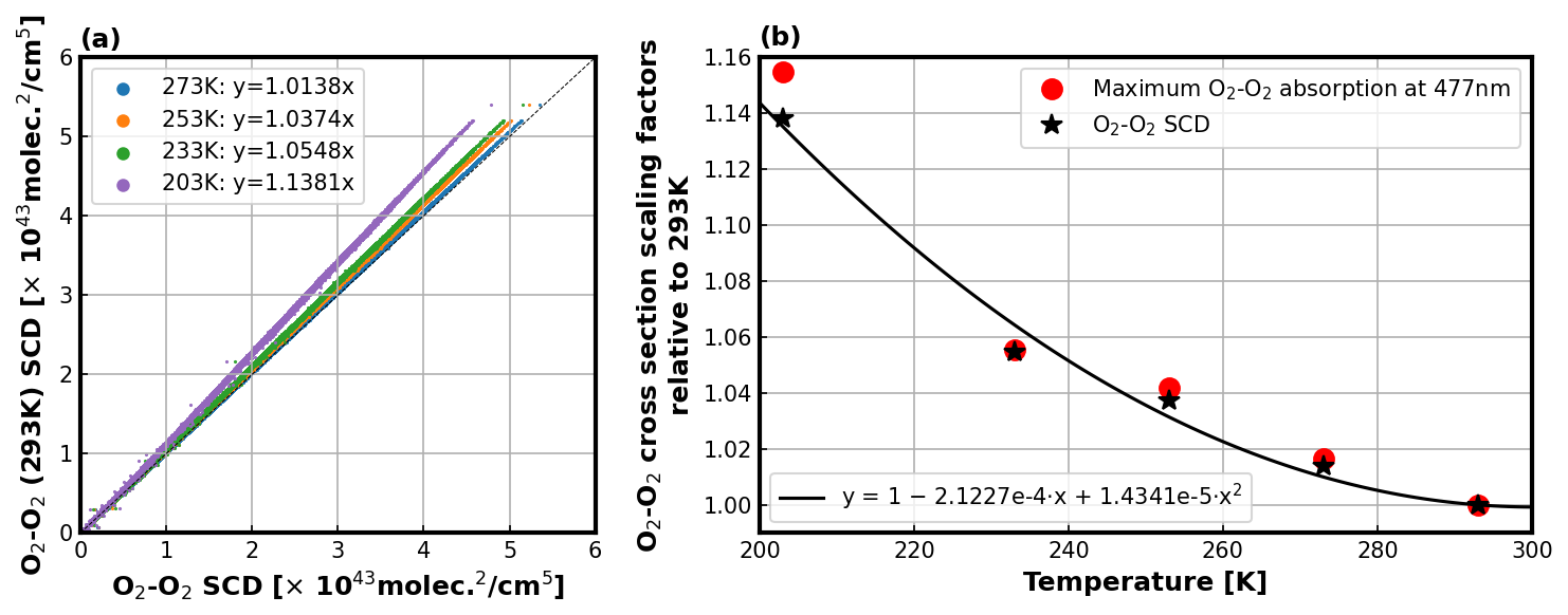
Figure 6Effect of temperature-dependent cross-sections on O2–O2 SCD retrieval. (a) Comparison of retrieved O2–O2 SCDs using the 293 K cross-section with those retrieved from cross-sections at various temperatures; (b) scaling factors for maximum O2–O2 absorption around 477 nm (red circles) and retrieved O2–O2 SCDs (black stars) at different temperatures relative to 293 K. The black line represents the fitted curve used to correct the temperature dependency of the O2–O2 cross-section based on the retrieved O2–O2 SCDs.
By fitting TROPOMI reflectance spectra with O2–O2 cross-sections measured at different temperatures, the retrieved O2–O2 SCDs exhibit a strong linear correlation, as shown in Fig. 6a. The scaling factors for the retrieved O2–O2 SCDs at different temperatures relative to 293 K closely match those obtained from the maximum O2–O2 absorption around 477 nm (see Fig. 6b). These scaling factors are then fitted to a quadratic polynomial (Fig. 6b) to characterize the temperature dependence of the O2–O2 absorption:
Here, T(p) represents the atmospheric temperature representative of satellite observations at pressure p, while T0 denotes the cross-section temperature used in the fit, fixed as 293 K. This correction factor is incorporated into the simulation of O2–O2 SCD (see Eq. 1) to align the simulated values with the SCDs derived from the DOAS fit. Subsequently, the calculation of γ is refined by explicitly considering the temperature dependence of the O2–O2 absorption cross-section, as follows:
where and represent the measured slant column and the slant column corresponding to the reference pressure-temperature profile, respectively. T(p) and Tref(p) denote the actual temperature profile and the temperature profile used to create the LUT, respectively.
The temperature correction factor is computed using LUTs for O2–O2 box-AMF and the corresponding reflectance to derive m(p). Additionally, our cloud retrieval algorithm performs three iterations to accurately determine the temperature correction factor for each observation. It is worth mentioning that, in our approach, the temperature correction for the O2–O2 cross-section must be accounted for in the calculation of O2–O2 VCD (see Eqs. 4 and 5) when creating the inverted LUT.
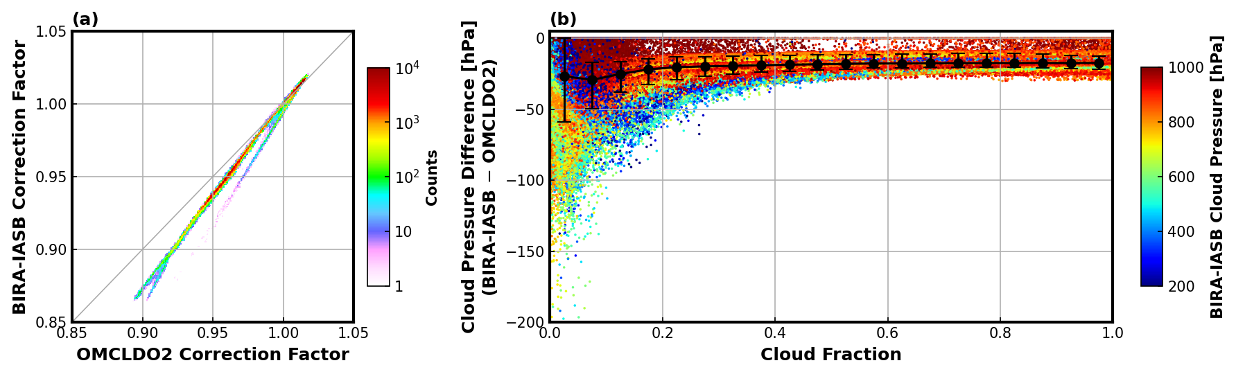
Figure 7Impact of temperature correction approaches. (a) Comparison of temperature correction factors calculated from BIRA-IASB and OMCLDO2 algorithms. The color bar indicates the sample counts. (b) Difference in the effective cloud pressure retrievals between the different temperature correction approaches (BIRA-IASB minus OMCLDO2), plotted against the effective cloud fraction. Both cloud retrievals implement the BIRA-IASB approach, with the temperature correction factor being the only parameter calculated separately using both the BIRA-IASB and OMCLDO2 methods. The color of the symbols represents the BIRA-IASB cloud pressures. The black circles indicate the median values within each 0.05 interval of cloud fraction, while the error bars represent the 10th and 90th percentiles of values within each bin. The analysis is based on TROPOMI measurements from orbit 5003 on 1 October 2018.
To assess the impact of the temperature correction factor on cloud retrieval, we consider data from a single orbit of TROPOMI data (orbit 5003 on 1 October 2018). Figure 7 compares temperature correction factors calculated using the BIRA-IASB and OMCLDO2 algorithms (Fig. 7a) and demonstrates their impact on cloud pressure retrieval (Fig. 7b). The BIRA-IASB approach includes both temperature-related factors described above, whereas the OMCLDO2 retrieval considers only the first factor. Accordingly, as shown in Fig. 7a, the BIRA-IASB temperature correction factors are stronger. The impact on the cloud fraction is negligible, whereas the effect on the cloud pressure is significant, as shown in Fig. 7b, which focuses on the differences in cloud pressure retrievals due to various temperature correction factors. Cloud pressures calculated with the BIRA-IASB correction factor systematically exhibit lower values, with differences increasing as cloud fractions decrease. The median difference ranges from 17 hPa for cloudy scenes to 30 hPa for nearly cloud-free scenes. The differences remain relatively small when the retrieved BIRA-IASB cloud pressure exceeds 900 hPa. Note that all cloud pressures in this analysis are capped at the surface pressure.
3.6 Surface albedo dataset
Surface albedo is an important parameter for accurately retrieving cloud properties. In the OMI OMCLDO2 product, surface albedo is derived from a 5-year climatology of the OMI LER (Veefkind et al., 2016), based on OMI L1b Collection 3 data, provided on a grid of 0.5° × 0.5° (Kleipool et al., 2008). Recently, a dedicated TROPOMI surface albedo climatology has been developed using TROPOMI measurements (Tilstra et al., 2024). This new climatology offers both a traditional LER and a directionally dependent LER (DLER), similar to the version derived from GOME-2 measurements by Tilstra et al. (2021), with a finer spatial resolution of 0.125° × 0.125°. The differences in the visible band between the OMI and TROPOMI LER databases are generally small, with a slightly high bias over high latitudes and some land regions (Tilstra et al., 2024). The DLER dataset has been implemented in version 2.4 of operational processing for cloud retrievals (FRESCO and OMCLDO2) and NO2 retrievals (van Geffen et al., 2022).
For OMI, the “mode LER” is used, representing the most frequently observed value derived through a statistical method, which is particularly effective for improving surface albedo retrieval over scenes with snow, ice, or desert cover (Kleipool et al., 2008). In contrast, for TROPOMI, the surface albedo is determined using the minimum surface LER for snow- and/or ice-free scenes, parameterized as a function of the viewing zenith angle (van Geffen et al., 2022). The OMI mode LER is systematically higher than the TROPOMI minimum LER, especially over bright surfaces (see Fig. A1), mainly due to differences in the statistical analysis methods used. Over land-covered surfaces, the TROPOMI DLER values at the east edge of the swath are 0.02–0.03 higher than those at the west edge of the swath and are comparable to OMI mode LER (Fig. 8). Over water surfaces, the DLER is identical to the corresponding LER, representing the diffuse component of reflection from the water surface (Tilstra et al., 2024).
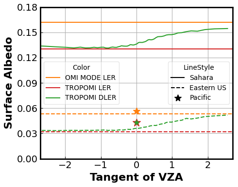
Figure 8Comparison of OMI mode LER, TROPOMI minimum LER for snow- and/or ice-free scenes, and DLER as a function of tan (θ) at 463 nm for the three surface types defined in Fig. A1. Note that the TROPOMI DLER retrieval is applied only to land-covered surface pixels.
The BIRA-IASB approach uses version 2.1 of the TROPOMI DLER dataset for retrievals in both OMI and TROPOMI, taking advantage of TROPOMI's overpass time, which closely aligns with that of OMI. Compared to version 1.0, which was used in the NO2 processor version 2.4 (van Geffen et al., 2024) and based on 3 years of Collection 1 L1 data; version 2.1 is based on 5 years of Collection 3 L1 data. It also includes enhancements for detecting and handling snow/ice contamination and excludes measurements affected by cloud shadows from the analysis (Tilstra et al., 2024). It should be noted that there are still some geometric differences between OMI and TROPOMI, which can introduce biases in DLER. Additionally, interannual variability is not accounted for. However, these differences are expected to be smaller than the discrepancy between OMI LER and TROPOMI LER in most scenarios, particularly for snow- and/or ice-free pixels.
In OMCLDO2 retrievals, surface albedo values are calculated as the average of the albedo at 463 and 494 nm (Boersma et al., 2007). In contrast, the BIRA-IASB approach directly uses albedo values from the surface albedo dataset at 463 nm, which is close to the center of the O2–O2 fitting window. Additionally, the current cloud retrieval approach is only valid when the surface albedo is below 0.6. As surface albedo approaches 0.8, the cloud retrieval becomes unstable, making it challenging for the algorithm to distinguish between clouds and the surface. This issue commonly occurs over snow- and ice-covered surfaces (Veefkind et al., 2016). In such cases, OMCLDO2 performs the retrieval using the LER method. This method models the scene by assuming a Lambertian surface that covers the entire pixel, fitting only the scene albedo and scene pressure. Consequently, it eliminates the need to distinguish between clouds and the surface. On the other hand, this study focuses on the cloud parameters for tropospheric trace gas retrievals in snow/ice-free scenes.
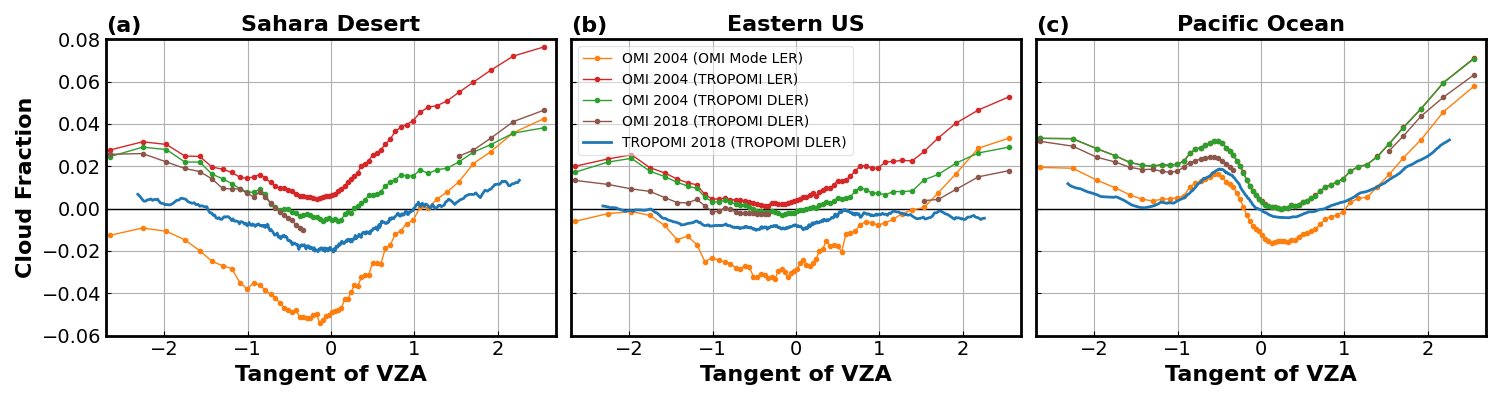
Figure 9Comparison of cloud fraction retrievals based on various surface albedo datasets as a function of tan (θ). The data presented in the figure represent the 1st percentile of retrieval values for each row across three selected regions (as defined in Fig. A1), based on 1 month of measurements in October. The sensors, measurement years, and surface albedo datasets (in brackets) are specified in the legend. Note that the TROPOMI LER surface albedo corresponds to TROPOMI DLER over the Pacific Ocean.
Figure 9 compares cloud fraction retrievals using various surface albedo datasets. Since cloud fraction retrievals can be influenced by variations in viewing geometries for cloudy scenes, we calculate the 1st percentile of cloud fraction values for each row to minimize the impact of clouds. These values, representing retrievals over cloud-free scenes, are plotted as a function of tan (θ). The results indicate that TROPOMI cloud fractions using TROPOMI DLER are generally close to 0, with slightly lower values at the nadir and relatively higher towards the edge of the swath, with minimal west–east bias. An exception is the enhancement around tan (θ) of −0.5 over the Pacific Ocean, attributed to sun-glint effects. OMI cloud fractions using TROPOMI DLER exhibit similar patterns to TROPOMI values but display a consistently high bias. The OMI cloud fraction values are comparable between 2004 (green) and 2018 (brown), except at the edges of the OMI swath over the eastern USA, where the 2004 values are relatively higher. This difference may be related to changes in land vegetation over time, which could have influenced the DLER values. When using TROPOMI LER, the cloud fractions are 0.02–0.04 higher on the east side of the OMI swath compared to those using TROPOMI DLER over land regions. In contrast, cloud fractions derived using OMI LER are systematically lower, particularly for nadir measurements.
Figure 10 presents examples of the global distribution of cloud fraction and cloud pressure retrieved from OMI and TROPOMI measurements using the BIRA-IASB approach. Since the algorithm is not sensitive under high surface albedo conditions, such as those in ice- or snow-covered areas in polar regions, the retrievals are limited to latitudes between 60° S and 60° N. The TROPOMI data are from 1 October 2018, while the OMI data include both 1 October 2018 and 1 October 2004. Missing data in the OMI maps for 1 October 2018 (gray regions) are primarily due to the OMI row anomaly. Additionally, cloud pressure retrievals are shown only for pixels with cloud fractions above 0.05.
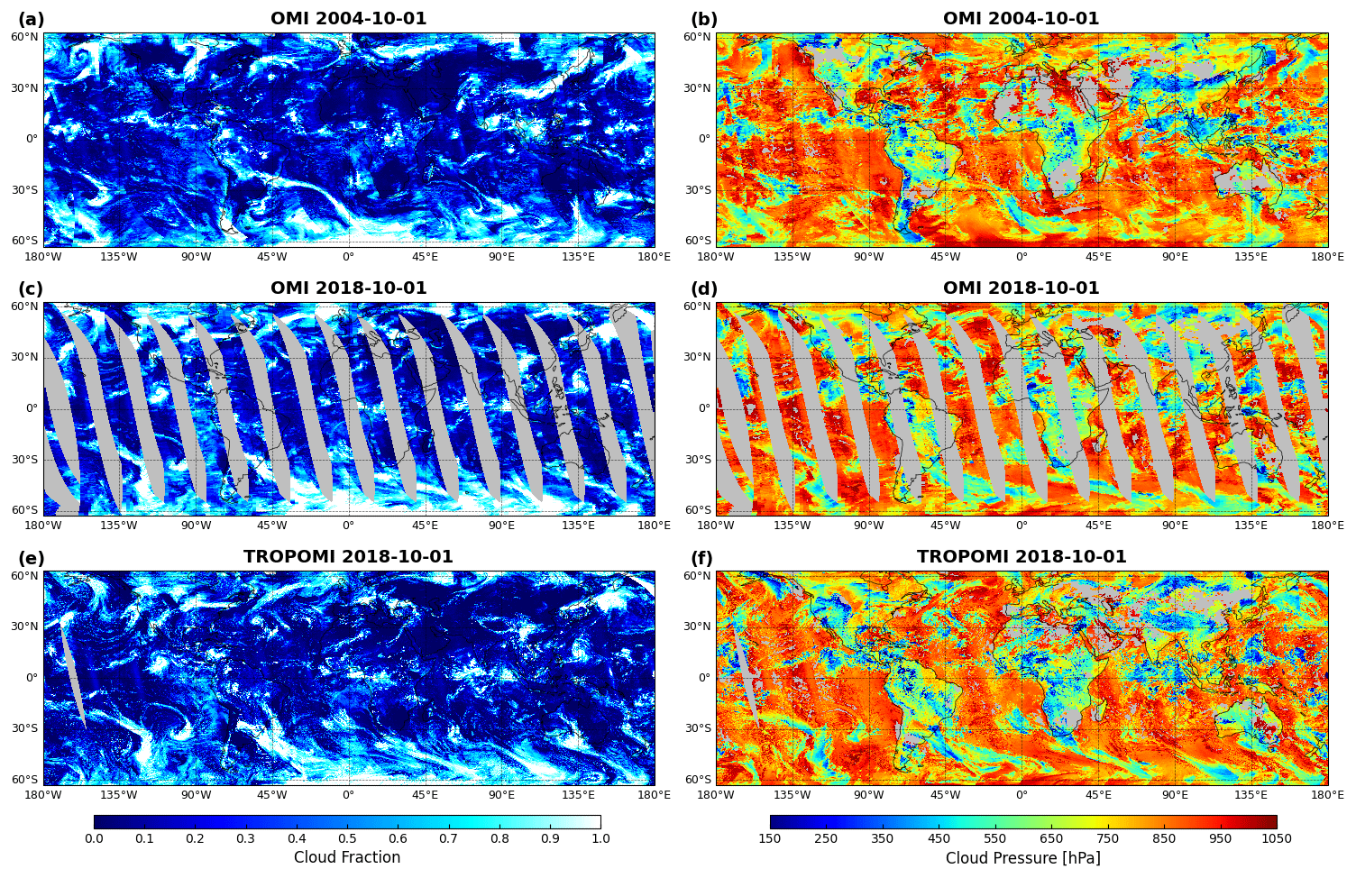
Figure 10Maps of BIRA-IASB O2–O2 cloud retrievals for OMI and TROPOMI. The top row (a, b) shows OMI retrievals for 1 October 2004, the middle row (c, d) displays OMI retrievals for 1 October 2018, and the bottom row (e, f) illustrates TROPOMI retrievals for 1 October 2018. The left column (a, c, e) depicts cloud fraction retrievals, while the right column (b, d, f) shows cloud pressure (in hPa) for regions where the cloud fraction > 0.05. Missing data for OMI on 1 October 2018 (gray areas) are due to the application of a row anomaly filter.
The BIRA-IASB cloud retrievals from OMI and TROPOMI on 1 October 2018 demonstrate a high degree of consistency. However, OMCLDO2 retrievals exhibit a systematic bias in cloud pressure, with OMI values being consistently lower (see Fig. A2). Despite being from different years, the cloud maps from OMI on 1 October 2004 also display a very similar distribution pattern. Most mid- to high- latitude regions are predominantly cloud-covered, while desert areas tend to have fewer clouds. Over ocean, cloud heights are generally lower (indicating higher cloud pressure), whereas they are significantly higher in the Intertropical Convergence Zone (ITCZ). Additionally, cloud heights tend to be greater over land compared to ocean. Over low-latitude ocean regions, distinct orbital structures are visible in the western part of the satellite swath, primarily due to sun-glint effects. These effects can lead the O2–O2 cloud retrieval to overestimate cloud fraction and potentially result in artificially low cloud pressure values.
To assess our retrieval algorithm, we first compare our retrievals with the OMCLDO2 products for both OMI and TROPOMI, investigate the impact of cloud corrections on NO2 retrievals, and finally evaluate the consistency of our retrievals between OMI and TROPOMI. The analysis is based on OMI measurements from October 2004 and October 2018, as well as TROPOMI measurements from October 2018. It is worth noting that tests were also conducted for other months, and the conclusions remained consistent.
4.1 Comparison with OMCLDO2
4.1.1 Overall performance
To evaluate our cloud algorithm, we compare the retrieved values of effective cloud fraction and effective cloud pressure with those from OMI OMCLDO2 version 2 (Veefkind et al., 2016), which have been newly processed using OMI Collection 4 data (Kleipool et al., 2022) with several improvements, as well as TROPOMI OMCLDO2 in the operational NO2 processing (van Geffen et al., 2022). Figure 11 presents comparison maps of cloud retrievals from OMI on 1 October 2004 and TROPOMI on 1 October 2018. Regardless of the date chosen, the comparison results are generally similar. The differences in cloud fraction generally do not exceed 0.01, with the BIRA-IASB values showing a slight positive bias, except for some pixels over East Asia and high latitudes. These discrepancies are likely due to differences in the surface albedo datasets used in the retrieval. Specifically, OMI OMCLDO2 uses the OMI climatological surface LER (Kleipool et al., 2008), TROPOMI OMCLDO2 uses the TROPOMI DLER v1.0 (van Geffen et al., 2024; Tilstra et al., 2024) (for processor versions 2.4.0), and our retrievals use the TROPOMI DLER v2.1 dataset. The difference between TROPOMI DLER v1.0 and v2.1 primarily arises from the treatment of snow/ice pixels. For cloud pressure, our OMI retrievals exhibit a higher bias compared to OMCLDO2, particularly in nearly cloud-free scenes over ocean. In contrast, our TROPOMI values are generally lower than those of OMCLDO2, especially over land, which helps bring OMI and TROPOMI cloud pressure retrievals closer to alignment.
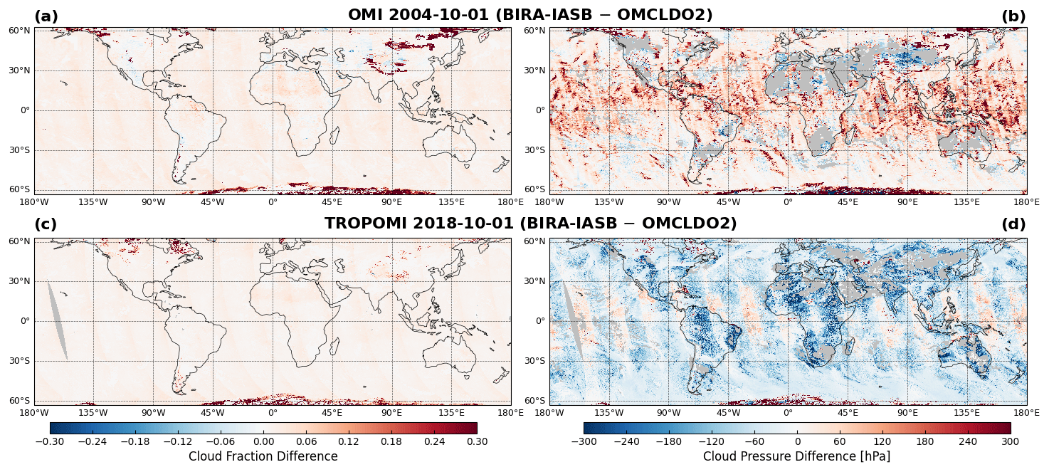
Figure 11Maps of cloud retrieval differences between BIRA-IASB and OMCLDO2 algorithms. The top row (a, b) shows OMI measurements from 1 October 2004, while the bottom row (c, d) presents TROPOMI measurements from 1 October 2018. The left column (a, c) depicts cloud fraction retrievals, while the right column (b, d) displays cloud pressure retrievals.
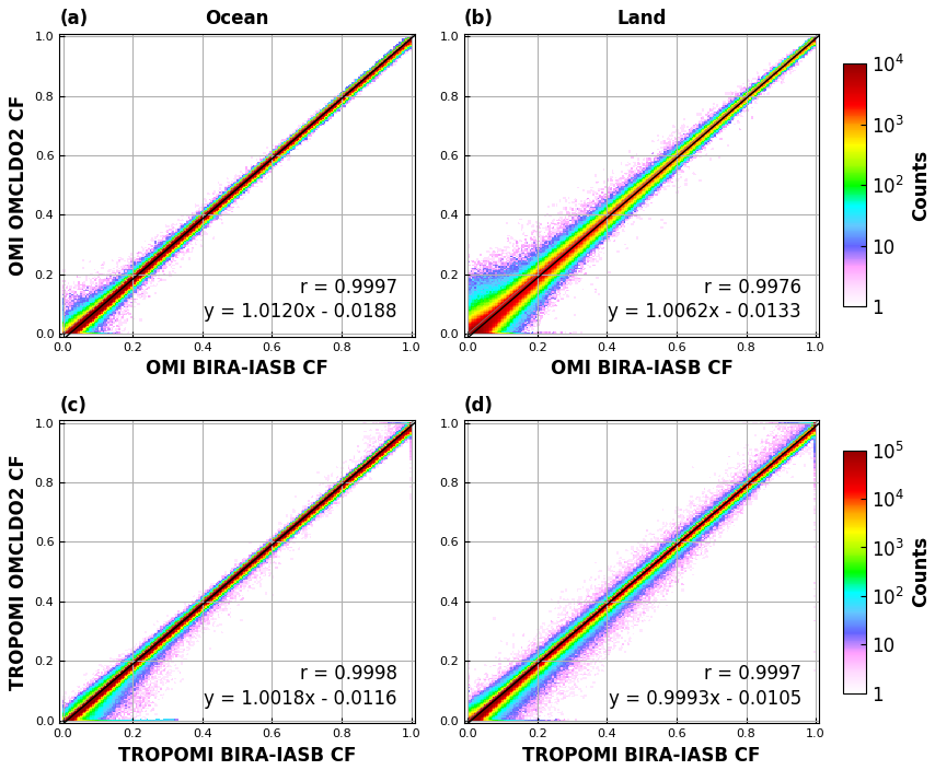
Figure 12Comparison of cloud fraction retrievals between BIRA-IASB and OMCLDO2 from 50° S to 50° N. The top panels (a, b) show OMI measurements from October 2004, while the bottom panels (c, d) show TROPOMI measurements from October 2018. The left panels (a, c) represent measurements over ocean, and the right panels (b, d) represent measurements over land. Sun-glint-affected pixels over ocean have been excluded from the analysis. The color bar indicates the sample counts, with the correlation coefficient and linear fit parameters provided in the legend.
Figure 12 shows scatter plots comparing cloud fraction retrieved using the OMCLDO2 algorithm with those obtained with our retrieval, for both ocean and land regions between 50° S and 50° N. This geographical range is selected to minimize the impact of snow/ice and large SZAs. The analysis is based on 1 month of OMI measurement from October 2004 and TROPOMI measurement from October 2018. The correlation coefficients between the two algorithms are close to 1, with a slightly lower value for OMI over land. The mean differences between the two datasets are less than 0.01 for all cloud fraction values. Significant differences in cloud fraction retrieval are mainly attributed to variations in the surface albedo used in the retrievals. Specifically, the relatively large scatter in low cloud fraction cases for OMI over land is attributed to the lack of consideration for geometry dependence in the OMI LER dataset. It is also worth noting that the BIRA-IASB approach retrieves cloud fraction at 465 nm using TOA reflectance, whereas OMCLDO2 retrieves it at 477 nm using continuum reflectance. The continuum reflectance is derived from the fitted polynomial of the DOAS results, representing reflectance without atmospheric absorption. However, these differences are expected to have a negligible impact on cloud fraction retrievals.
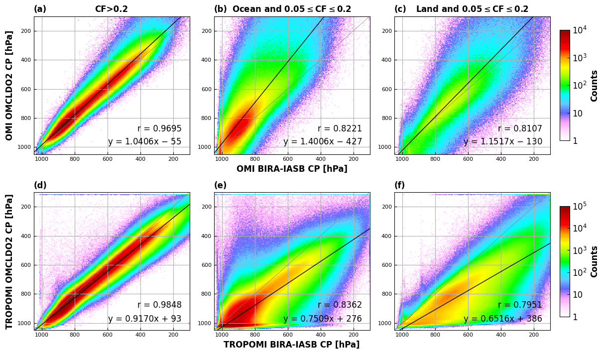
Figure 13Comparison of cloud pressure retrievals between BIRA-IASB and OMCLDO2. The top row (a–c) shows OMI measurements from October 2004, while the bottom row (d–f) shows TROPOMI measurements from October 2018. The analysis includes measurements over cloudy scenes (a, d), ocean–clear scenes (b, e), and land–clear scenes (c, f). Measurements with cloud fractions below 0.05 in either retrieval have been excluded. The color bar indicates sample counts, and the correlation coefficient along with linear fit parameters are provided in the legend.
Figure 13 presents scatter plots of cloud pressures calculated with OMCLDO2 compared to those calculated using our approach, based on 1 month of OMI and TROPOMI measurements. Tropospheric NO2 retrieval from satellite measurements typically excludes pixels affected by clouds. Such pixels are defined as having a cloud radiance fraction greater than 0.5, which corresponds to an effective cloud fraction of approximately 0.15–0.2. Therefore, the analysis is categorized into several scenarios: scenes with significant cloud cover (cloud fraction > 20 %) and scenes with low cloud fraction (cloud fraction ≤ 20 %), with the latter further categorized by surface type as either over ocean or over land. For cloudy scenes, the slopes of linear fits are approximately 1.04 for OMI and 0.92 for TROPOMI, with small offsets. This indicates that BIRA-IASB cloud pressures are generally higher for OMI and lower for TROPOMI. The data exhibit low scatter for high-cloud-pressure cases, with slightly increased scatter for low-cloud-pressure cases. In contrast, cloud-free scenes exhibit significantly more scatter, and the mean differences are relatively larger than those observed for cloudy scenes. For OMI data over land, however, the mean differences are comparable, with BIRA-IASB retrievals showing a slight negative bias for high cloud pressures and a positive bias for low cloud pressures.
Table 2Impact of the key improvements in the BIRA-IASB cloud retrieval compared to the OMCLDO2 approach, as well as the overall differences between the two retrievals. For each improvement, the BIRA-IASB retrieval is applied, and the cloud pressure difference resulting from the individual change is calculated. The analysis is based on 1 d of OMI (1 October 2004) and TROPOMI (1 October 2018) measurements, restricted to snow- and/or ice-free pixels within the 50° S to 50° N latitude range.
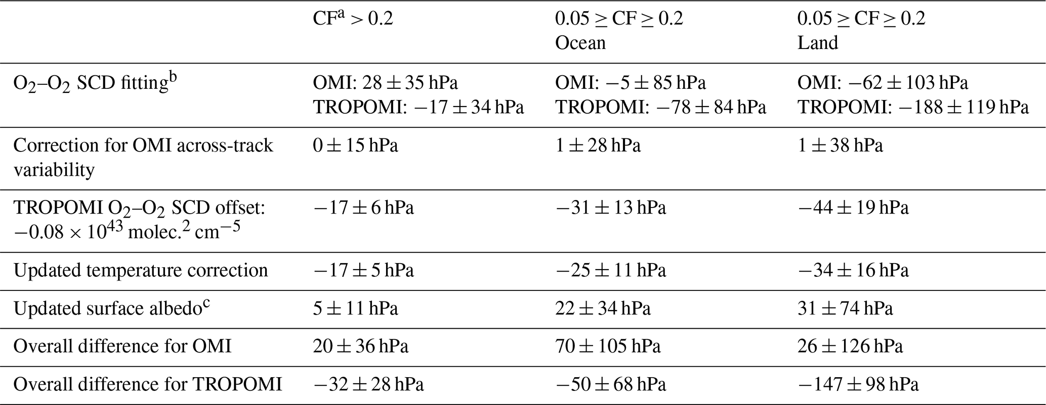
a Cloud fraction (CF) is from the BIRA-IASB retrieval. b Wavelength dependence due to the use of different fitting windows between the BIRA-IASB and OMCLDO2 retrievals is not accounted for. c Comparison between use of OMI minimum LER (Kleipool et al., 2008) and TROPOMI DLER (Tilstra et al., 2024).
Table 2 summarizes the impact of each improvement in our cloud pressure retrieval relative to OMCLDO2, as well as the overall differences between the two retrieval approaches, based on 1 d of OMI and TROPOMI data. Effects on cloud fraction are not included, as the implemented changes have minimal influence in this regard. The impact is generally much greater in scenes with low cloud fraction than in cloudy conditions, and it tends to be more pronounced over land than over ocean. The results indicate that the most significant discrepancies primarily stem from differences in the DOAS fitting settings, particularly for TROPOMI. Although this analysis does not account for the wavelength dependence introduced by using different fitting windows in the O2–O2 SCD retrieval, the impact of this effect is relatively minor.
4.1.2 Across-track dependence
Synthetic analysis indicates that the O2–O2 cloud retrieval is sensitive to both solar radiation and viewing geometries (Wang et al., 2020; Yu et al., 2022). This section examines the across-track dependencies of the BIRA-IASB and OMCLDO2 cloud products for OMI and TROPOMI, displayed as monthly mean cloud fractions and cloud heights plotted against tan (θ), as shown in Fig. 14. The analysis is based on measurements collected over ocean and land between 50° S and 50° N latitudes, with a VZA of less than 60°. Additionally, pixels with a cloud fraction below 0.05 are excluded from the cloud pressure analysis to avoid high uncertainty in cloud height at very low cloud fractions. The dataset includes OMI measurements from October 2004 and October 2018, as well as TROPOMI measurements from October 2018. The retrieved cloud fraction is constrained between 0 and 1, while the cloud pressure is limited to values between 150 hPa and the surface pressure.
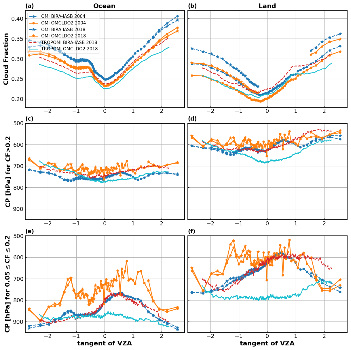
Figure 14Across-track dependence of monthly mean cloud retrievals from OMI and TROPOMI for October, based on the measurements between 50° S and 50° N latitudes. The left panels (a, c, e) present results over ocean, while the right panels (b, d, f) show results over land. The analysis includes cloud fraction (a, b), cloud pressure (CP) in cloudy scenes (c, d), and cloud pressure in low cloud fraction scenes (e, f). The legend details the sensors, retrieval methods, and time periods included in the analysis.
Figure 14 shows that the mean cloud fractions over ocean are slightly higher compared to land. The cloud fraction values increase towards the edges of the swath, likely due to factors such as geometric effects and enhanced cloud scattering along the slant path. Over ocean, a peak is observed in the sun-glint region, located west of the swath's center, whereas over land an enhancement is also evident east of the middle row. This enhancement is also reflected in the dependence on reflectance values, becoming more pronounced over land and for high clouds (not shown). Further investigation is required to fully understand this behavior, but it is beyond the scope of this study. The cloud fractions from the different products exhibit similar patterns, with slight offsets. The BIRA-IASB cloud fraction values are higher than those from OMCLDO2, with the difference ranging from approximately 0.015 at nadir to 0.03 at the edge of the swath. The difference in OMI cloud fractions between 2004 and 2018 is minimal over ocean, while over land the 2018 values are 0.02–0.03 higher compared to 2004. This difference may be attributed to changes in surface albedo or atmospheric scattering (e.g., aerosols) between 2004 and 2018. OMI cloud fractions are consistently higher than those from TROPOMI. Although the solar radiation geometries of OMI and TROPOMI are not identical, the observed differences in cloud fractions cannot be fully explained by these geometric variations alone.
The mean cloud pressure values are generally higher over ocean compared to land. For cloudy scenes (cloud fraction > 0.2), OMI retrievals show a weak dependence on VZA for OMI, while TROPOMI retrieves slightly higher cloud pressures near nadir, with values increasing towards the edges of the swath. The mean cloud pressure values from two TROPOMI products are closely aligned on the west side of the swath, whereas on the east side of the swath, the BIRA-IASB cloud pressures are generally higher than those from OMCLDO2. However, no clear west-to-east trend is observed between the two OMI retrievals.
For scenes with low cloud fraction, cloud pressure retrievals exhibit significantly stronger across-track variation compared to cloudy scenes. In such cases, the OMI BIRA-IASB cloud pressure values are generally higher than those of OMCLDO2, while for TROPOMI the BIRA-IASB values tend to be lower. Most cloud pressure retrievals exhibit a consistent broadly across-track pattern, typically with lower values near nadir that decrease towards the edges of the swath. An exception is noted for the TROPOMI OMCLDO2 retrieval over land, where cloud pressures at nadir are slightly higher than those at the swath edges. Over ocean, the OMI and TROPOMI BIRA-IASB retrievals exhibit a consistent across-track behavior. Over land, however, discrepancies arise near the swath edges, likely caused by surface reflectance anisotropy effects resulting from slight differences in solar radiation and viewing geometries between OMI and TROPOMI. Additionally, OMI OMCLDO2 cloud pressures exhibit pronounced across-track variability due to the lack of a de-striping correction, resulting in amplitudes exceeding 100 hPa in certain rows. The difference between the retrievals from 2004 and 2018 is minimal, indicating temporal stability in these features.
4.1.3 Comparison of zonal means
In this section, zonal mean comparisons are presented for the various cloud products. Figure 15 shows the monthly zonal mean cloud retrievals for OMI in October 2004 and TROPOMI in October 2018. Both cloud fraction and cloud pressure retrievals demonstrate similar latitudinal patterns across the different cloud products. The left panel shows that cloud fractions tend to be lower at low latitudes, with a slight increase around 5 to 10° N, and gradually increase towards higher latitudes. Differences between the products are generally within 0.05, with slightly larger discrepancies observed between 20° S and 10° N, as well as at high latitudes. In the cloud pressure comparison (right panel), lower cloud pressures are observed in tropical regions, increasing towards higher latitudes. The OMI OMCLDO2 values are consistently lower, while TROPOMI OMCLDO2 values are generally higher, with BIRA-IASB cloud pressures typically falling in between. The difference between OMI OMCLDO2 and TROPOMI OMCLDO2 ranges from 50 to 150 hPa. BIRA-IASB cloud pressures from the two sensors show good overall agreement, with slightly larger differences observed in regions at latitudes 35–15° S and 10–30° N.
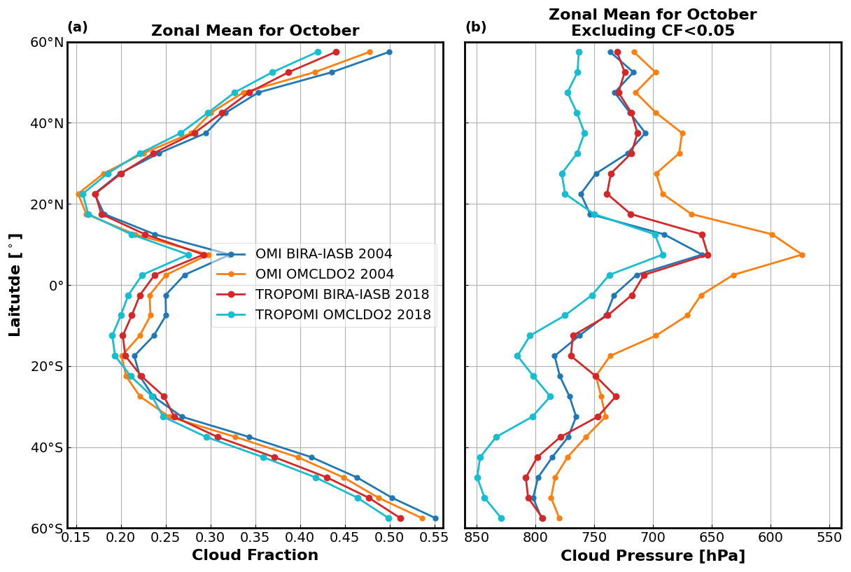
Figure 15Monthly zonal mean cloud retrievals for OMI (October 2004) and TROPOMI (October 2018), derived from measurements with a VZA less than 60°: (a) cloud fraction and (b) cloud pressure. To ensure reliable cloud pressure comparisons, pixels with a cloud fraction below 0.05 are excluded, as very low cloud fractions lead to high uncertainties in cloud pressure retrievals. The legend provides details on sensors, retrieval methods, and time periods used in the analysis.
4.1.4 Dependence of cloud pressure on cloud fraction
To further analyze the difference between BIRA-IASB and OMCLDO2 cloud retrievals, Fig. 16 presents the mean cloud pressures as a function of effective cloud fraction. Measurements with retrieved cloud fractions below 0.01 are excluded from the analysis due to the high uncertainty in cloud pressure retrieval under these conditions. Over ocean, the mean cloud pressures are below 700 hPa for fully cloudy scenes across all retrievals, increasing as cloud fractions decrease. The differences between cloud products are within 15 hPa for large cloud fractions but grow slightly as cloud fractions decrease. These differences become significant for nearly cloud-free scenes, with OMCLDO2 cloud pressure reaching as high as 950 hPa for TROPOMI compared to as low as 700 hPa for OMI. Over the land, the averaged cloud pressure exhibits only minor variations in different cloud fractions, except for cloud fractions below 0.2. In these low cloud fraction cases, similar to observations over ocean, the OMCLDO2 cloud pressure is higher for TROPOMI and lower for OMI, with the two BIRA-IASB cloud pressures falling in between. Additionally, these two BIRA-IASB cloud products exhibit strong agreement in their values, demonstrating consistent dependence over both land and ocean.
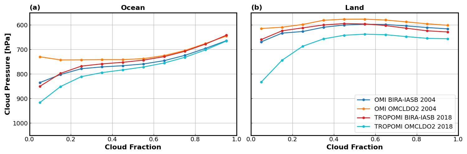
Figure 16Dependence of monthly mean cloud pressures on cloud fractions over ocean (a) and land (b). The analysis uses OMI and TROPOMI measurements for latitudes between 50° S and 50° N for the month of October. The legend provides details on the sensors, cloud retrieval methods, and time periods used in the analysis.
4.2 Cloud effects on the NO2 retrieval
The satellite NO2 retrieval algorithm employs the DOAS approach, which consists of three main steps: (1) the NO2 SCDs are retrieved by spectral fitting within a predefined wavelength window, matching the satellite-measured reflectance spectrum to a set of relevant reference spectra; (2) the stratospheric contribution is estimated and removed from the NO2 slant column; and (3) the residual tropospheric slant column is converted into a VCD using a tropospheric AMF. Cloud retrievals mainly influence the calculation of the AMF, which relies on the independent pixel approximation (IPA). The AMF is expressed as a linear combination of clear-sky and cloudy AMFs, with the retrieved cloud fraction and cloud pressure used to determine the cloudy AMF.
In this study, we use the OMI QA4ECV NO2 product version 1.1 (Boersma et al., 2018) and the TROPOMI operational NO2 product version 2.4 (van Geffen et al., 2022) to evaluate the impact of changes in cloud correction methods on the derived tropospheric NO2 VCDs. The NO2 SCDs and stratospheric components are directly obtained from these products, while the calculation of the NO2 AMF follows the approach described in Boersma et al. (2004), using scripts developed at BIRA-IASB. The box-AMF and TOA reflectance LUTs are pre-calculated at 437.5 nm using VLIDORT v2.8. Surface albedo data are taken from the TROPOMI DLER climatology dataset v2.1 at 440 nm, and a priori NO2 profiles are obtained from the TM5-MP model (Williams et al., 2017), providing vertical profiles simulated at a 1°×1° spatial resolution for 34 atmospheric layers, ranging from the surface up to 0.1 hPa.
Figure 17 presents monthly mean tropospheric NO2 VCDs from OMI and TROPOMI, using BIRA-IASB cloud corrections, for October 2018. The lower noise level of TROPOMI is evident, particularly for low NO2 levels, such as over ocean. Note that approximately half of the OMI measurements are excluded from the analysis due to a detector row anomaly (Dobber et al., 2008). Overall, we observe a good agreement in both the magnitude and spatial distribution of the NO2 columns.
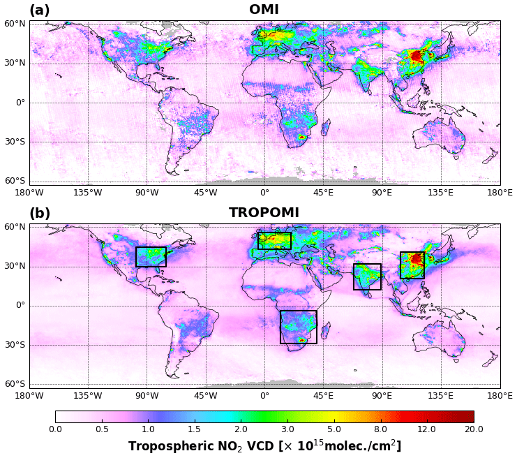
Figure 17Average tropospheric NO2 VCD retrieved from OMI (a) and TROPOMI (b) using BIRA-IASB O2–O2 cloud correction for October 2018. These data are gridded at a spatial resolution of 0.5°, considering only observations with a cloud radiance fraction below 50 %. The large black boxes on the TROPOMI map represent regions used for comparison (see Fig. 18).
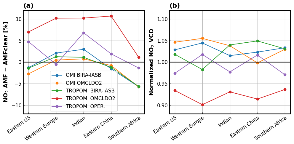
Figure 18Impact of cloud corrections on NO2 retrievals. (a) Difference between the cloud-corrected AMF and the clear-sky AMF; (b) difference in NO2 VCD retrievals using the cloud-corrected AMF compared to those using the clear-sky AMF. Each NO2 VCD value is normalized by the average of the five products for the corresponding region. Data analysis is based on monthly average maps for October 2018 over selected regions, as shown in Fig. 17. The colors represent NO2 AMF calculations using various cloud correction methods and different sensors, while the x axis indicates the selected regions.
The uncertainty in the tropospheric NO2 is primarily driven by spectral fitting uncertainty in clean areas, whereas in regions with high NO2 columns the uncertainty is largely dominated by the estimation of the tropospheric AMF (Boersma et al., 2004). For quantitative comparisons, we calculate the monthly-averaged AMFs and NO2 columns for five regions (large black boxes in Fig. 17) representing some of the most polluted areas globally. To assess the impact of cloud corrections on NO2 retrievals, we compare the cloud-corrected AMFs with the clear-sky AMFs, as well as the NO2 retrievals using AMFs with and without cloud correction; results are presented in Fig. 18. In addition to the BIRA-IASB and OMCLDO2 clouds, the analysis implements the cloud correction approach used in the TROPOMI operational NO2 product. This correction is based on an effective cloud fraction calculated in the NO2 fitting window at 440 nm, combined with a cloud pressure derived from the dedicated TROPOMI FRESCO-S algorithm (version 2.4; van Geffen et al., 2022). As shown in Fig. A3, the 440 nm cloud fractions agree well with the results from our O2–O2 algorithm. In contrast, the cloud fractions derived from the O2–O2 and O2–A band measurements exhibit larger discrepancies, and these differences are particularly evident for low cloud fractions, with differences more pronounced over land. For cloudy scenes, there is generally good agreement in cloud pressure retrieval between our O2–O2 results and FRESCO (Fig. A4). However, in scenes with low cloud fractions, the figures show substantial scatter. FRESCO tends to retrieve relatively lower cloud pressure for high cloud cases over ocean and slightly higher over land.
The impact of cloud corrections on the NO2 AMF is generally within ±20 % (see Fig. A5). All corrections exhibit a systematic positive bias over ocean, whereas over land the effect is comparatively minor, except in tropical regions, where most cloud products introduce a negative bias. As shown in Fig. 18a, the average impact of cloud correction for the selected polluted regions ranges from −6 % to 11 %, depending on the cloud product used. The AMF difference resulting from various cloud corrections can exceed 10 %. However, these values remain well below the typical uncertainty associated with tropospheric NO2 AMFs (Boersma et al., 2004). The AMFs show little variation when using OMI BIRA-IASB, OMI OMCLDO2, or TROPOMI BIRA-IASB cloud corrections. However, the AMF obtained with the TROPOMI OMCLDO2 cloud correction is systematically higher compared to the others, while the AMF based on the cloud correction used in the TROPOMI operational process generally falls between these values, except for a deviation in Western Europe. Additionally, the cloud correction effect over Southern Africa is smaller compared to other regions, likely due to the relatively higher clouds in this area. The NO2 VCDs generally exhibit an inverse relationship with the effect of cloud corrections, particularly for the three TROPOMI retrievals. This correlation is somewhat weaker when comparing OMI and TROPOMI, which may be influenced by sampling differences between the two sensors. The difference in NO2 VCDs resulting from the use of different cloud corrections can be as large as 15 %. In general, the TROPOMI NO2 retrieval based on BIRA-IASB cloud correction aligns more closely with OMI NO2 retrievals compared to TROPOMI NO2 retrievals using other correction methods.
4.3 Comparison between OMI and TROPOMI
In this section, we assess the consistency of BIRA-IASB cloud retrievals between OMI and TROPOMI. Additionally, we compare NO2 retrievals that utilize the cloud correction based on the BIRA-IASB cloud products. The analysis relies on OMI and TROPOMI measurements from October 2018. To illustrate the improved consistency achieved with the new cloud retrievals, the OMCLDO2 cloud retrievals are also included in the analysis.
4.3.1 Clouds
Figure 19 shows scatter plots of gridded cloud fraction and cloud pressure retrievals from OMI and TROPOMI for October 2018. For each TROPOMI orbit, the corresponding OMI measurement with an overpass time difference of less than 50 min is selected. The data are gridded on a resolution of 0.5° × 0.5°, considering only ground pixels with latitude ≤ 50°. For cloud fraction comparison, only grid cells with valid measurements covering more than 75 % of the cells are included in the analysis. For cloud pressure comparison, the cloud pressure values are computed as the average of all pressures within each grid cell, weighted by cloud fraction. Grid cells with an average cloud fraction below 0.05 or valid measurement coverage of less than 75 % are excluded from the analysis.
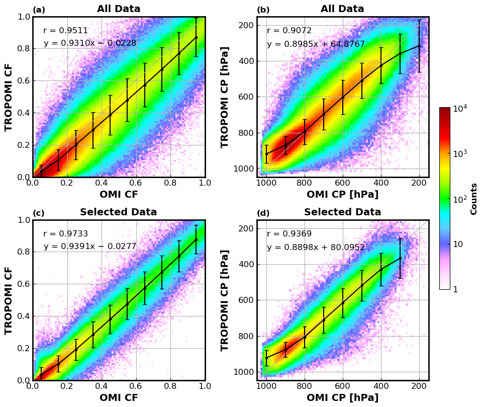
Figure 19Scatter plots of the OMI and TROPOMI gridded cloud parameters for October 2018 (panels (a) and (c): cloud fraction, panels (b) and (d): cloud pressures). The top panels (a, b) include all matched pixels with latitude < 50°, while the bottom panels (c, d) include only the pixels with observation times differing by less than 15 min between OMI and TROPOMI, restricted to measurements form the west side of the satellite swath. For cloud pressure comparisons, cloud pressure values are weighted by cloud fraction, and grid cells with cloud fractions below 0.05 are excluded. The correlation coefficient and linear fit coefficients are presented in the legend, and black circles with error bars represent the binned average values, along with their standard deviations. Refer to the main text for further details.
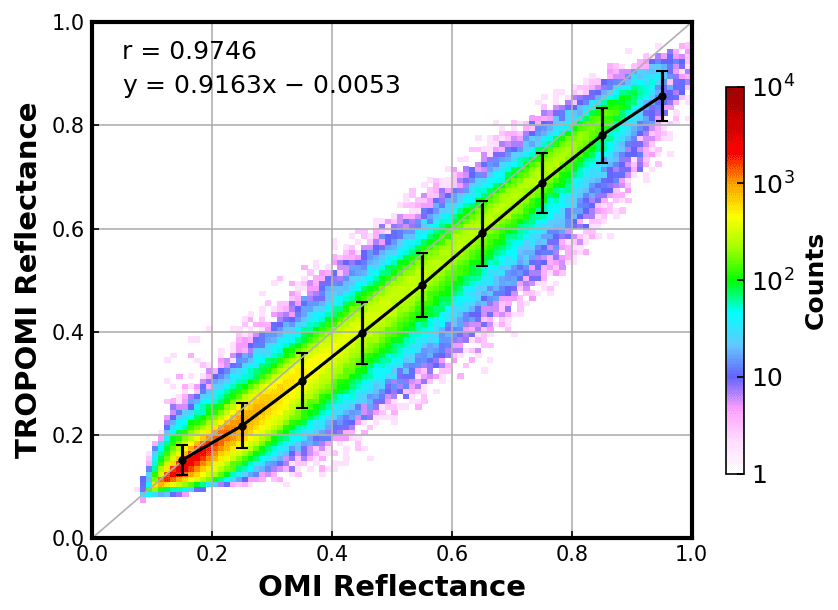
Figure 20Similar to Fig. 19, this figure presents a scatter plot of OMI and TROPOMI reflectance for October 2018, including pixels between 50° S and 50° N. The correlation coefficient and linear fit parameters are provided in the legend.
The results show generally good agreement for both cloud fraction and cloud pressure comparisons. Figure 19a shows a linear fit for cloud fraction, with a slope of 0.93, an offset of −0.02, and a correlation coefficient of 0.95 between the two datasets. The binned average values reveal a consistent bias between OMI and TROPOMI, which decreases slightly as the cloud fractions approach zero. This difference is primarily due to discrepancies in the L1 reflectances, as shown in Fig. 20. However, this bias is challenging to correct with a simple linear fit to align the two sensors, as it depends not only on radiance or irradiance but also varies with sensor rows (as discussed in Sect. 4.1.2). The cloud pressure comparison (Fig. 19b) shows a linear fit with a slope of 0.9, an offset of 65 hPa, and a correlation coefficient of 0.91. The binned averages demonstrate a high level of agreement, except for very low (< 350 hPa) or very high (> 950 hPa) cloud pressures, where OMI cloud pressures are biased low for low pressures and high for high pressures compared to TROPOMI. When stricter data selection criteria are applied, such as reducing the overpass time difference to less than 15 min (instead of 50 min) and considering only west-side satellite measurements, as shown in Fig. 19c and d, the data exhibit reduced scatter. However, the mean differences remain largely consistent with previous results. The conclusions remain valid across different time periods, as shown in Fig. A6. For OMCLDO2, the cloud fraction differences between OMI and TROPOMI are comparable to those observed using the BIRA-IASB approach. However, larger discrepancies are evident in cloud pressure when it is below 900 hPa, as shown in Fig. A7.
4.3.2 NO2
To evaluate the consistency of tropospheric NO2 VCDs between OMI and TROPOMI, we use NO2 retrievals with various cloud corrections obtained from Sect. 4.2, and we grid the data following the approach described in Sect. 4.3.1. It should be noted that only NO2 data from pixels having a cloud radiance fraction below 50 % are included in the analysis.
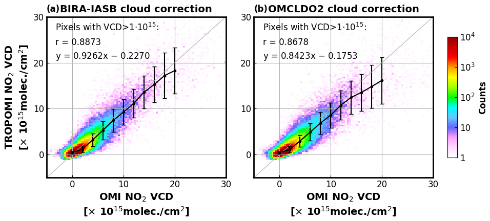
Figure 21Scatter plots of the OMI and TROPOMI gridded NO2 tropospheric VCDs for October 2018, considering only the ground pixels with a cloud radiance fraction below 50 % and latitudes between 50° S and 50° N. Black circles with error bars represent the binned average values, along with their standard deviations. The correlation coefficient and linear fit parameters are provided in the legend. The NO2 retrievals are based on the cloud correction using cloud information from the BIRA-IASB approach (a) and the OMCLDO2 approach (b).
The comparison of NO2 retrievals between OMI and TROPOMI is shown in Fig. 21. Retrievals using BIRA-IASB and OMCLDO2 cloud corrections generally show good agreement between the two sensors. More specifically, the binned average data show minimal differences in NO2 retrievals using the BIRA-IASB cloud correction, with OMI NO2 columns generally being slightly higher. This bias is more pronounced for high NO2 levels. The differences in NO2 retrievals based on OMCLDO2 cloud correction are slightly larger compared to those using BIRA-IASB. Since clouds primarily affect the estimation of the NO2 AMF, the accuracy of the cloud correction significantly influences NO2 retrievals, particularly in polluted conditions. To further evaluate this, a linear fit is applied to the NO2 data for retrieved values greater than 1 × 10¹⁵ molec. cm−2 for both sensors. Compared to the retrievals using OMCLDO2 cloud correction, the BIRA-IASB correction increases the TROPOMI NO2 VCDs, aligning them more closely with OMI values. This correction has the potential to improve the validation results for TROPOMI NO2 (Judd et al., 2020; Lange et al., 2023). The other time periods have been analyzed, as shown in Fig. A8. While the agreement between OMI and TROPOMI shows a slight seasonal variation, the NO2 retrievals based on the BIRA-IASB correction consistently demonstrate better agreement than those using the OMCLDO2 correction.
We have developed a new cloud retrieval algorithm based on the O2–O2 absorption band at 477 nm. Compared to the operational O2–O2 cloud algorithm OMCLOD2, our retrieval introduces several main improvements: (1) the DOAS slant column fitting employs a larger fitting window, capturing both O2–O2 absorption bands at 446 and 477 nm; (2) a de-striping correction is applied to reduce across-track variability; (3) an SCD offset of −0.08 × 1043 molec.2 cm−5 is applied in the TROPOMI retrieval to improve consistency with OMI measurements; (4) a temperature correction accounts for the temperature dependence of the O2–O2 cross-section; and (5) consistent auxiliary data, such as atmospheric information and surface albedo, are used for both OMI and TROPOMI sensors. This new cloud algorithm is designed for use in tropospheric trace gas retrievals from UV–Visible sensors, currently optimized for snow- and ice-free conditions.
We evaluate our cloud algorithm by comparing the retrieved cloud fraction and cloud pressure values with those from the latest version of the OMI and TROPOMI OMCLDO2 products. The results demonstrate good agreement in cloud fraction retrievals, with an average difference of up to 0.01. However, discrepancies are observed in cloud pressure values, with our retrievals generally higher than OMCLDO2 for OMI and lower for TROPOMI. The discrepancies become more pronounced in nearly cloud-free conditions or in scenarios with low cloud pressure. The improved DOAS slant column retrieval approach, incorporating offset correction, improves the alignment of our TROPOMI cloud retrievals with those of OMI compared to OMCLDO2. Additionally, the de-striping correction significantly reduces the across-track variability for OMI. However, differences in cloud pressure retrievals exhibit varying west–east biases. The dependence of cloud pressures on cloud fractions shows similar patterns across all cloud products, except in cases with small cloud fractions. When comparing OMI and TROPOMI, our retrievals show excellent agreement in both cloud fraction and cloud pressure, although a systematic bias of 0.05 in cloud fractions is observed. This bias is attributed to differences in L1b data between the two sensors.
We apply the new cloud algorithm to NO2 retrievals and analyze changes in NO2 columns resulting from different cloud correction methods. Overall, the NO2 maps from OMI and TROPOMI show good agreement when using our cloud correction method. Over polluted regions, the cloud correction impacts the calculation of NO2 AMFs, resulting in an average difference ranging from −6 % to 11 %, depending on the cloud correction method and the specific region. The differences in AMF due to varying cloud corrections can exceed 10 %, and NO2 retrievals based on TROPOMI OMCLDO2 cloud correction are systematically lower than those using other cloud correction methods. Additionally, NO2 VCDs from OMI and TROPOMI using our cloud correction align more closely with the 1 : 1 line compared to those obtained using the OMCLDO2 cloud correction.
Future work should incorporate error estimation for the retrieval results to better quantify uncertainties. To address snow and ice conditions, the retrieval should be extended to retrieve scene parameters (scene albedo and scene pressure). Once the full TROPOMI and OMI data records are processed, product stability should be assessed, and comprehensive validation studies conducted. Additionally, the algorithm could be adapted for application with other sensors, such as GEMS, TEMPO, and GOME-2, as well as other trace gases as products (HCHO, SO2, CHOCHO). Finally, the long-term impact of cloud parameters on tropospheric trace gas retrievals should be investigated to evaluate the importance of cloud corrections, and the consistency of these corrections across different sensors should be assessed.
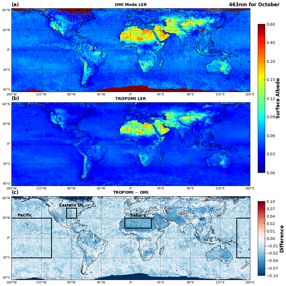
Figure A1Monthly surface albedo climatology at 463 nm for October, derived from 5 years of TROPOMI (a) and OMI (b) measurements, along with the difference between TROPOMI and OMI (c). The three large black boxes on the difference map indicate different surface types: desert (Sahara), forest/agriculture (Eastern US), and ocean (Pacific).
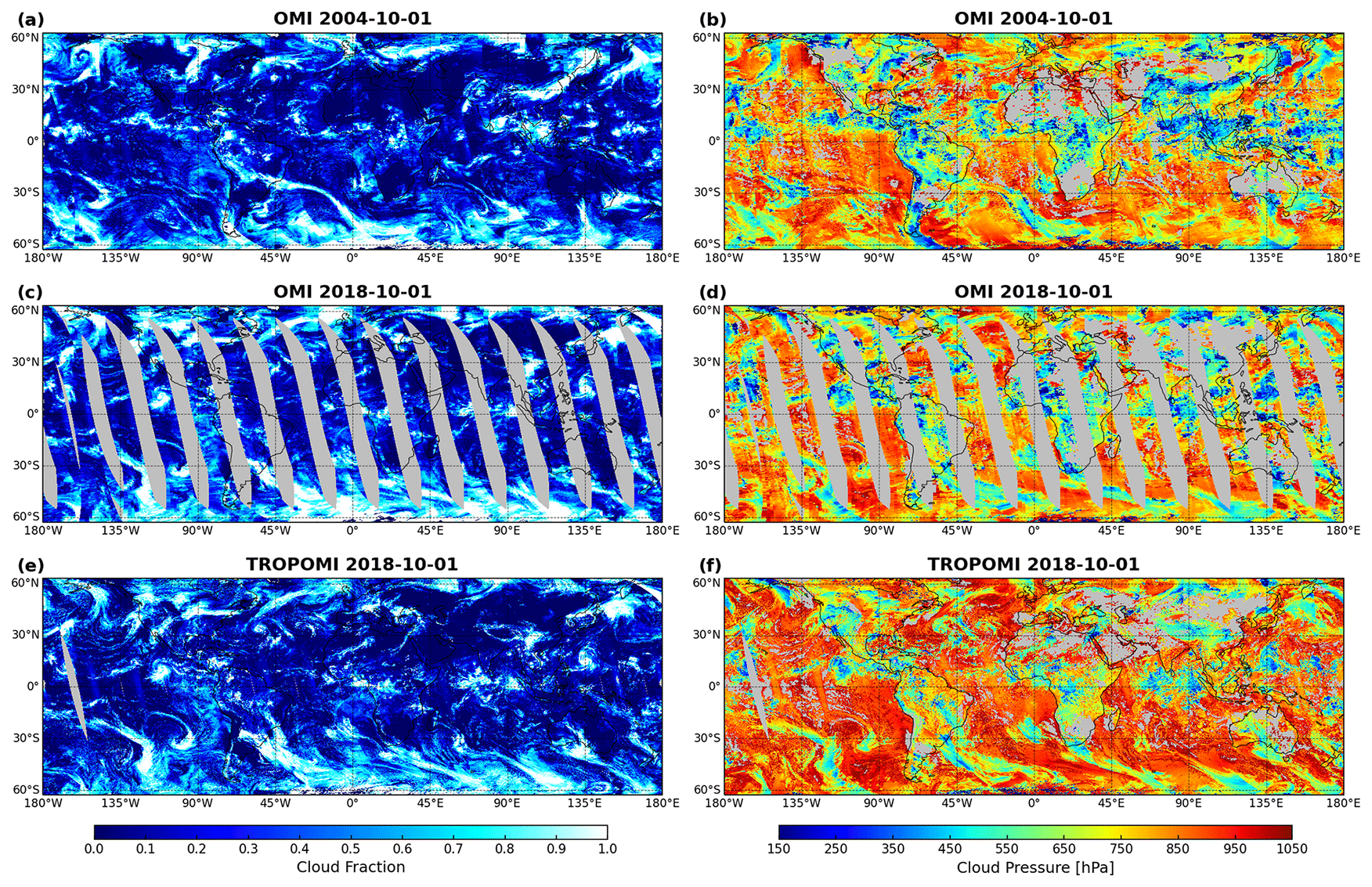
Figure A2Similar to Fig. 10 but for OMCLDO2 retrieval.
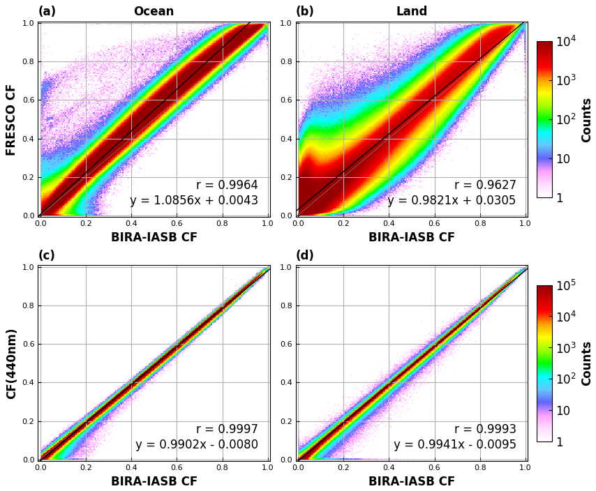
Figure A3Similar to Fig. 12 but showing a comparison between our TROPOMI O2–O2 cloud fraction retrievals with FRESCO (a, b), as well as the 440 nm cloud fraction (c, d) used in the operational TROPOMI NO2 retrieval.
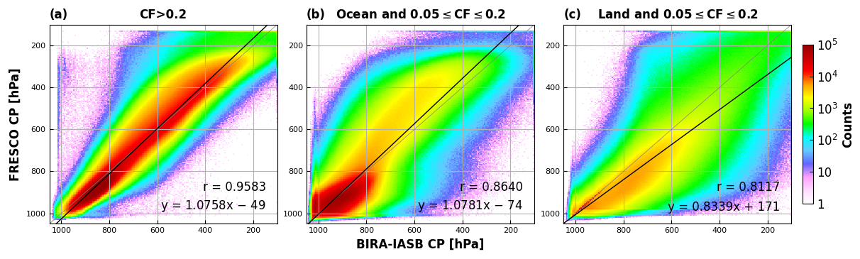
Figure A4Similar to Fig. 13 but for comparison of TROPOMI cloud pressure retrievals between BIRA-IASB O2–O2 and FRESCO.
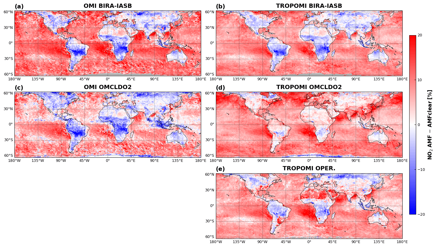
Figure A5Monthly average impact of cloud corrections on the tropospheric NO2 retrievals from OMI (a, c) and TROPOMI for October 2018. The NO2 AMF is calculated using identical retrieval settings, differing only in the cloud correction approach applied. Data are gridded at a spatial resolution of 0.5°, including only observations with a cloud radiance fraction below 0.5.
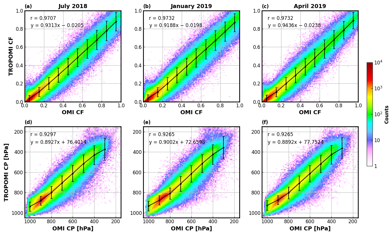
Figure A6Similar to Fig. 19c and d but based on measurements from July 2018, January 2019, and April 2019.
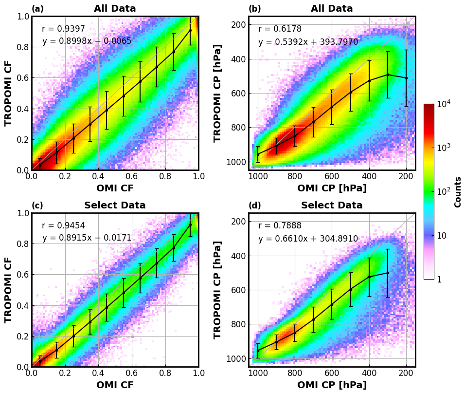
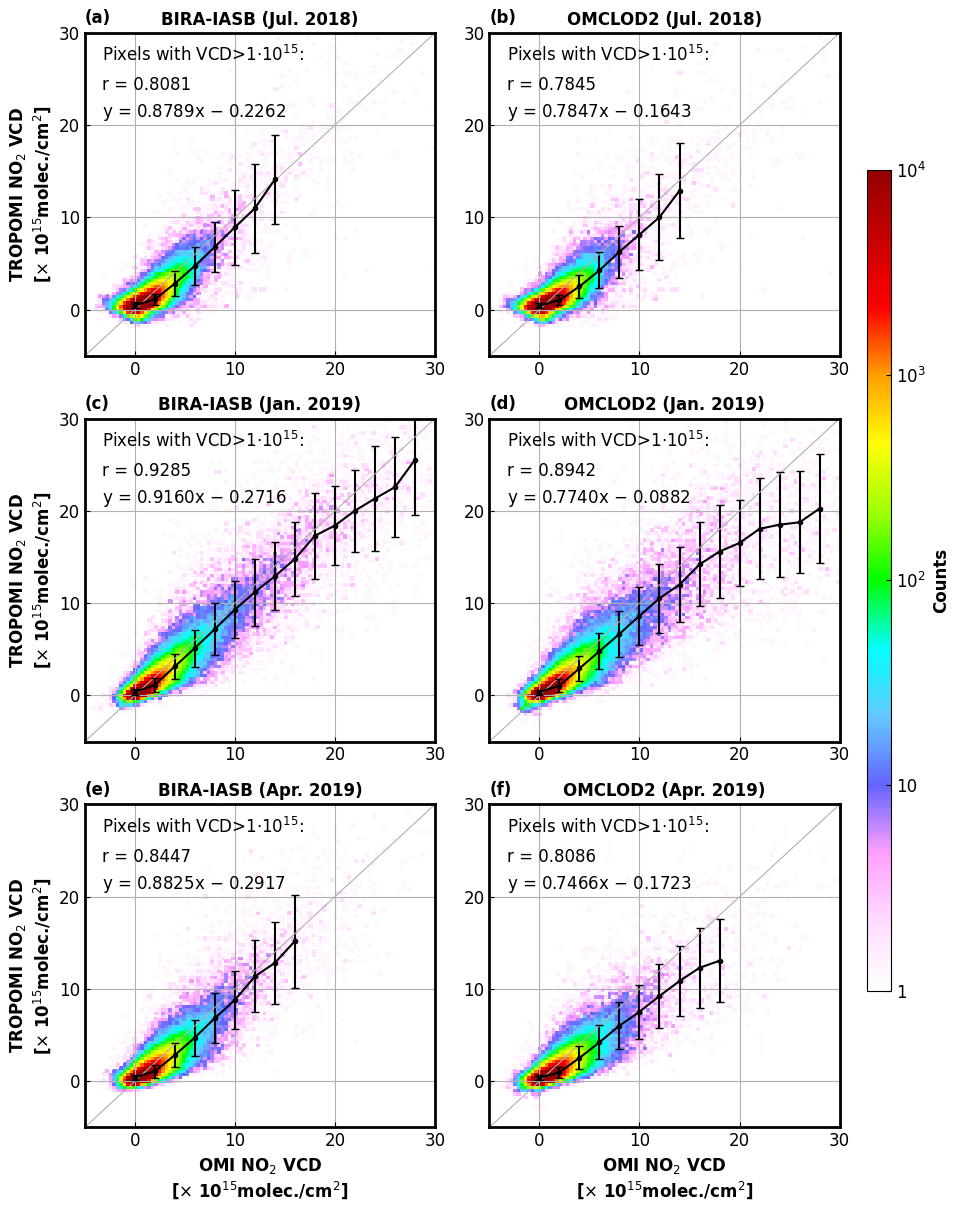
The BIRA-IASB O2–O2 cloud datasets presented in the study are available upon request. The QDOAS software for DOAS retrieval of trace gases is available from https://uv-vis.aeronomie.be/software/QDOAS/ (Danckaert et al., 2017). The OMI Level 1b Collection 4 product is available at https://disc.gsfc.nasa.gov/datasets/ (last access: 30 August 2025, Kleipool et al., 2022; DOIs: https://doi.org/10.5067/AURA/OMI/DATA1401, Kleipool, 2021a, and https://doi.org/10.5067/AURA/OMI/DATA1404, Kleipool, 2021b). The OMI Level 2 Collection 4 cloud data files are available upon request from Maarten Sneep at KNMI, and OMI/QA4ECV NO2 data are available via the QA4ECV portal (https://www.temis.nl/qa4ecv/no2.html, last access: 30 August 2025). TROPOMI operational products including L1, L2, and auxiliary data are downloaded via ESA's Copernicus Data Space Ecosystem (https://dataspace.copernicus.eu/, last access: 30 August 2025, Ludewig et al., 2020; DOIs: L1b: https://doi.org/10.5270/S5P-mhtbru8, Copernicus Sentinel-5P, 2021a, and https://doi.org/10.5270/S5P-kb39wni, Copernicus Sentinel-5P, 2021b; NO2 L2 data: https://doi.org/10.5270/S5P-9bnp8q8, van Geffen et al., 2020; Copernicus Sentinel-5P, 2021c). The TROPOMI surface DLER database is available at the TEMIS website (https://www.temis.nl/surface/albedo/, Tilstra et al., 2024). CAMS model data are retrieved from the CAMS Atmosphere Data Store (https://ads.atmosphere.copernicus.eu, last access: 30 August 2025, Inness et al., 2019; DOI: https://doi.org/10.24381/d58bbf47, Copernicus Atmosphere Monitoring Service, 2020).
HY is the main contributor to the study; he developed the cloud retrieval algorithm, applied it to the satellite observations, and led the writing of this paper. IDS and MVR provided technical support for satellite retrievals, while NT, MS, and PV contributed to the conceptualization and methodology. All co-authors participated in discussions of the results and contributed to the writing of this article.
At least one of the (co-)authors is a member of the editorial board of Atmospheric Measurement Techniques. The peer-review process was guided by an independent editor, and the authors also have no other competing interests to declare.
Publisher's note: Copernicus Publications remains neutral with regard to jurisdictional claims made in the text, published maps, institutional affiliations, or any other geographical representation in this paper. While Copernicus Publications makes every effort to include appropriate place names, the final responsibility lies with the authors.
This work contains modified S5P TROPOMI L1b data post-processed by BIRA-IASB. We thank Antje Ludewig for providing the annual-averaged OMI solar irradiance spectrum from 2005 and for sharing valuable insights on OMI and TROPOMI L1 data. We also acknowledge the use of OMI OMCLDO2 data provided by KNMI and offer our thanks to Robert Spurr for making the VLIDORT model available.
This research has been supported by the Belgian Federal Science Policy Office (Belgian PRODEX TRACE-S5P projects) and the European Space Agency (ESA Precursors_cci+ project (grant no. 4000138243/22/I-NB)).
This paper was edited by Jian Xu and reviewed by three anonymous referees.
Acarreta, J. R., De Haan, J. F., and Stammes, P.: Cloud pressure retrieval using the O2-O2 absorption band at 477 nm, J. Geophys. Res.-Atmos., 109, D05204, https://doi.org/10.1029/2003jd003915, 2004. a, b, c, d, e
Aliwell, S. R., Van Roozendael, M., Johnston, P. V., Richter, A., Wagner, T., Arlander, D. W., Burrows, J. P., Fish, D. J., Jones, R. L., Tørnkvist, K. K., Lambert, J.-C., Pfeilsticker, K., and Pundt, I.: Analysis for BrO in zenith-sky spectra: An intercomparison exercise for analysis improvement, J. Geophys. Res.-Atmos., 107, ACH 10-1–ACH 10-20, https://doi.org/10.1029/2001JD000329, 2002. a, b
Bauwens, M., Compernolle, S., Stavrakou, T., Müller, J.-F., van Gent, J., Eskes, H., Levelt, P. F., van der A, R., Veefkind, J. P., Vlietinck, J., Yu, H., and Zehner, C.: Impact of Coronavirus Outbreak on NO2 Pollution Assessed Using TROPOMI and OMI Observations, Geophys. Res. Lett., 47, e2020GL087978, https://doi.org/10.1029/2020GL087978, 2020. a
Boersma, K. F., Eskes, H. J., and Brinksma, E. J.: Error analysis for tropospheric NO2 retrieval from space, J. Geophys. Res.-Atmos., 109, D04311, https://doi.org/10.1029/2003jd003962, 2004. a, b, c, d, e, f
Boersma, K. F., Eskes, H. J., Veefkind, J. P., Brinksma, E. J., van der A, R. J., Sneep, M., van den Oord, G. H. J., Levelt, P. F., Stammes, P., Gleason, J. F., and Bucsela, E. J.: Near-real time retrieval of tropospheric NO2 from OMI, Atmos. Chem. Phys., 7, 2103–2118, https://doi.org/10.5194/acp-7-2103-2007, 2007. a, b, c, d
Boersma, K. F., Eskes, H. J., Dirksen, R. J., van der A, R. J., Veefkind, J. P., Stammes, P., Huijnen, V., Kleipool, Q. L., Sneep, M., Claas, J., Leitão, J., Richter, A., Zhou, Y., and Brunner, D.: An improved tropospheric NO2 column retrieval algorithm for the Ozone Monitoring Instrument, Atmos. Meas. Tech., 4, 1905–1928, https://doi.org/10.5194/amt-4-1905-2011, 2011. a, b, c
Boersma, K. F., Eskes, H. J., Richter, A., De Smedt, I., Lorente, A., Beirle, S., van Geffen, J. H. G. M., Zara, M., Peters, E., Van Roozendael, M., Wagner, T., Maasakkers, J. D., van der A, R. J., Nightingale, J., De Rudder, A., Irie, H., Pinardi, G., Lambert, J.-C., and Compernolle, S. C.: Improving algorithms and uncertainty estimates for satellite NO2 retrievals: results from the quality assurance for the essential climate variables (QA4ECV) project, Atmos. Meas. Tech., 11, 6651–6678, https://doi.org/10.5194/amt-11-6651-2018, 2018. a
Bucsela, E. J., Krotkov, N. A., Celarier, E. A., Lamsal, L. N., Swartz, W. H., Bhartia, P. K., Boersma, K. F., Veefkind, J. P., Gleason, J. F., and Pickering, K. E.: A new stratospheric and tropospheric NO2 retrieval algorithm for nadir-viewing satellite instruments: applications to OMI, Atmos. Meas. Tech., 6, 2607–2626, https://doi.org/10.5194/amt-6-2607-2013, 2013. a
Chambers, L. H., Wielicki, B. A., and Evans, K. F.: Accuracy of the independent pixel approximation for satellite estimates of oceanic boundary layer cloud optical depth, J. Geophys. Res.-Atmos., 102, 1779–1794, https://doi.org/10.1029/96JD02995, 1997. a
Chance, K. V. and Spurr, R. J. D.: Ring effect studies: Rayleigh scattering, including molecular parameters for rotational Raman scattering, and the Fraunhofer spectrum, Appl. Opt., 36, 5224–5230, https://doi.org/10.1364/AO.36.005224, 1997. a
Clémer, K., Van Roozendael, M., Fayt, C., Hendrick, F., Hermans, C., Pinardi, G., Spurr, R., Wang, P., and De Mazière, M.: Multiple wavelength retrieval of tropospheric aerosol optical properties from MAXDOAS measurements in Beijing, Atmos. Meas. Tech., 3, 863–878, https://doi.org/10.5194/amt-3-863-2010, 2010. a
Copernicus Atmosphere Monitoring Service: CAMS global reanalysis (EAC4), Copernicus Atmosphere Monitoring Service (CAMS) Atmosphere Data Store [data set], https://doi.org/10.24381/d58bbf47, 2020. a
Copernicus Sentinel-5P: TROPOMI Level 1B Irradiance products, Version 02, European Space Agency [data set], https://doi.org/10.5270/S5P-mhtbru8, 2021a. a
Copernicus Sentinel-5P: TROPOMI Level 1B Radiance products, Version 02, European Space Agency [data set], https://doi.org/10.5270/S5P-kb39wni, 2021b. a
Copernicus Sentinel-5P: TROPOMI Level 2 Nitrogen Dioxide total column products, Version 02, European Space Agency [data set], https://doi.org/10.5270/S5P-9bnp8q8, 2021c. a
Danckaert, T., Fayt, C., Van Roozendael, M., De Smedt, I., Letocart, V., Merlaud, A., and Pinardi, G.: QDOAS Software User Manual, Version 3.2, Tech. rep., Royal Belgian Institute for Space Aeronomy, https://uv-vis.aeronomie.be/software/QDOAS/QDOAS_manual.pdf (last access: 30 August 2025), 2017 (software available at: https://uv-vis.aeronomie.be/software/QDOAS/, last access: 30 August 2025). a, b, c, d
De Smedt, I., Stavrakou, T., Hendrick, F., Danckaert, T., Vlemmix, T., Pinardi, G., Theys, N., Lerot, C., Gielen, C., Vigouroux, C., Hermans, C., Fayt, C., Veefkind, P., Müller, J.-F., and Van Roozendael, M.: Diurnal, seasonal and long-term variations of global formaldehyde columns inferred from combined OMI and GOME-2 observations, Atmos. Chem. Phys., 15, 12519–12545, https://doi.org/10.5194/acp-15-12519-2015, 2015. a
De Smedt, I., Pinardi, G., Vigouroux, C., Compernolle, S., Bais, A., Benavent, N., Boersma, F., Chan, K.-L., Donner, S., Eichmann, K.-U., Hedelt, P., Hendrick, F., Irie, H., Kumar, V., Lambert, J.-C., Langerock, B., Lerot, C., Liu, C., Loyola, D., Piters, A., Richter, A., Rivera Cárdenas, C., Romahn, F., Ryan, R. G., Sinha, V., Theys, N., Vlietinck, J., Wagner, T., Wang, T., Yu, H., and Van Roozendael, M.: Comparative assessment of TROPOMI and OMI formaldehyde observations and validation against MAX-DOAS network column measurements, Atmos. Chem. Phys., 21, 12561–12593, https://doi.org/10.5194/acp-21-12561-2021, 2021. a
Dobber, M., Kleipool, Q., Dirksen, R., Levelt, P., Jaross, G., Taylor, S., Kelly, T., Flynn, L., Leppelmeier, G., and Rozemeijer, N.: Validation of Ozone Monitoring Instrument level 1b data products, J. Geophys. Res.-Atmos., 113, D15S06, https://doi.org/10.1029/2007JD008665, 2008. a, b
Finkenzeller, H. and Volkamer, R.: O2–O2 CIA in the gas phase: Cross-section of weak bands, and continuum absorption between 297–500 nm, J. Quant. Spectrosc. Ra., 279, 108063, https://doi.org/10.1016/j.jqsrt.2021.108063, 2022. a
Gordon, I., Rothman, L., Hargreaves, R., Hashemi, R., Karlovets, E., Skinner, F., Conway, E., Hill, C., Kochanov, R., Tan, Y., Wcisło, P., Finenko, A., Nelson, K., Bernath, P., Birk, M., Boudon, V., Campargue, A., Chance, K., Coustenis, A., Drouin, B., Flaud, J., Gamache, R., Hodges, J., Jacquemart, D., Mlawer, E., Nikitin, A., Perevalov, V., Rotger, M., Tennyson, J., Toon, G., Tran, H., Tyuterev, V., Adkins, E., Baker, A., Barbe, A., Canè, E., Császár, A., Dudaryonok, A., Egorov, O., Fleisher, A., Fleurbaey, H., Foltynowicz, A., Furtenbacher, T., Harrison, J., Hartmann, J., Horneman, V., Huang, X., Karman, T., Karns, J., Kassi, S., Kleiner, I., Kofman, V., Kwabia–Tchana, F., Lavrentieva, N., Lee, T., Long, D., Lukashevskaya, A., Lyulin, O., Makhnev, V., Matt, W., Massie, S., Melosso, M., Mikhailenko, S., Mondelain, D., Müller, H., Naumenko, O., Perrin, A., Polyansky, O., Raddaoui, E., Raston, P., Reed, Z., Rey, M., Richard, C., Tóbiás, R., Sadiek, I., Schwenke, D., Starikova, E., Sung, K., Tamassia, F., Tashkun, S., Vander Auwera, J., Vasilenko, I., Vigasin, A., Villanueva, G., Vispoel, B., Wagner, G., Yachmenev, A., and Yurchenko, S.: The HITRAN2020 molecular spectroscopic database, J. Quant. Spectrosc. Ra., 277, 107949, https://doi.org/10.1016/j.jqsrt.2021.107949, 2022. a
Inness, A., Ades, M., Agustí-Panareda, A., Barré, J., Benedictow, A., Blechschmidt, A.-M., Dominguez, J. J., Engelen, R., Eskes, H., Flemming, J., Huijnen, V., Jones, L., Kipling, Z., Massart, S., Parrington, M., Peuch, V.-H., Razinger, M., Remy, S., Schulz, M., and Suttie, M.: The CAMS reanalysis of atmospheric composition, Atmos. Chem. Phys., 19, 3515–3556, https://doi.org/10.5194/acp-19-3515-2019, 2019. a
Joiner, J. and Vasilkov, A.: First results from the OMI rotational Raman scattering cloud pressure algorithm, IEEE T. Geosci. Remote, 44, 1272–1282, https://doi.org/10.1109/TGRS.2005.861385, 2006. a
Judd, L. M., Al-Saadi, J. A., Szykman, J. J., Valin, L. C., Janz, S. J., Kowalewski, M. G., Eskes, H. J., Veefkind, J. P., Cede, A., Mueller, M., Gebetsberger, M., Swap, R., Pierce, R. B., Nowlan, C. R., Abad, G. G., Nehrir, A., and Williams, D.: Evaluating Sentinel-5P TROPOMI tropospheric NO2 column densities with airborne and Pandora spectrometers near New York City and Long Island Sound, Atmos. Meas. Tech., 13, 6113–6140, https://doi.org/10.5194/amt-13-6113-2020, 2020. a
Kleipool, Q.: OMI/Aura Level 1B Averaged Solar Irradiances V004, Goddard Earth Sciences Data and Information Services Center (GES DISC) [data set], https://doi.org/10.5067/Aura/OMI/DATA1401, 2021a. a
Kleipool, Q.: OMI/Aura Level 1B VIS Global Geolocated Earthshine Radiances V004, Goddard Earth Sciences Data and Information Services Center (GES DISC) [data set], https://doi.org/10.5067/AURA/OMI/DATA1404, 2021b. a
Kleipool, Q., Ludewig, A., Babić, L., Bartstra, R., Braak, R., Dierssen, W., Dewitte, P.-J., Kenter, P., Landzaat, R., Leloux, J., Loots, E., Meijering, P., van der Plas, E., Rozemeijer, N., Schepers, D., Schiavini, D., Smeets, J., Vacanti, G., Vonk, F., and Veefkind, P.: Pre-launch calibration results of the TROPOMI payload on-board the Sentinel-5 Precursor satellite, Atmos. Meas. Tech., 11, 6439–6479, https://doi.org/10.5194/amt-11-6439-2018, 2018. a
Kleipool, Q., Rozemeijer, N., van Hoek, M., Leloux, J., Loots, E., Ludewig, A., van der Plas, E., Adrichem, D., Harel, R., Spronk, S., ter Linden, M., Jaross, G., Haffner, D., Veefkind, P., and Levelt, P. F.: Ozone Monitoring Instrument (OMI) collection 4: establishing a 17-year-long series of detrended level-1b data, Atmos. Meas. Tech., 15, 3527–3553, https://doi.org/10.5194/amt-15-3527-2022, 2022. a, b, c, d
Kleipool, Q. L., Dobber, M. R., de Haan, J. F., and Levelt, P. F.: Earth surface reflectance climatology from 3 years of OMI data, J. Geophys. Res.-Atmos., 113, D18308, https://doi.org/10.1029/2008JD010290, 2008. a, b, c, d
Koelemeijer, R. B., Stammes, P., Hovenier, J. W., and De Haan, J. F.: A fast method for retrieval of cloud parameters using oxygen a band measurements from the Global Ozone Monitoring Experiment, J. Geophys. Res.-Atmos., 106, 3475–3490, https://doi.org/10.1029/2000JD900657, 2001. a
Krijger, J. M., van Weele, M., Aben, I., and Frey, R.: Technical Note: The effect of sensor resolution on the number of cloud-free observations from space, Atmos. Chem. Phys., 7, 2881–2891, https://doi.org/10.5194/acp-7-2881-2007, 2007. a
Lange, K., Richter, A., Schönhardt, A., Meier, A. C., Bösch, T., Seyler, A., Krause, K., Behrens, L. K., Wittrock, F., Merlaud, A., Tack, F., Fayt, C., Friedrich, M. M., Dimitropoulou, E., Van Roozendael, M., Kumar, V., Donner, S., Dörner, S., Lauster, B., Razi, M., Borger, C., Uhlmannsiek, K., Wagner, T., Ruhtz, T., Eskes, H., Bohn, B., Santana Diaz, D., Abuhassan, N., Schüttemeyer, D., and Burrows, J. P.: Validation of Sentinel-5P TROPOMI tropospheric NO2 products by comparison with NO2 measurements from airborne imaging DOAS, ground-based stationary DOAS, and mobile car DOAS measurements during the S5P-VAL-DE-Ruhr campaign, Atmos. Meas. Tech., 16, 1357–1389, https://doi.org/10.5194/amt-16-1357-2023, 2023. a
Latsch, M., Richter, A., Eskes, H., Sneep, M., Wang, P., Veefkind, P., Lutz, R., Loyola, D., Argyrouli, A., Valks, P., Wagner, T., Sihler, H., van Roozendael, M., Theys, N., Yu, H., Siddans, R., and Burrows, J. P.: Intercomparison of Sentinel-5P TROPOMI cloud products for tropospheric trace gas retrievals, Atmos. Meas. Tech., 15, 6257–6283, https://doi.org/10.5194/amt-15-6257-2022, 2022. a
Levelt, P., van den Oord, G., Dobber, M., Malkki, A., Visser, H., de Vries, J., Stammes, P., Lundell, J., and Saari, H.: The ozone monitoring instrument, IEEE T. Geosci. Remote, 44, 1093–1101, https://doi.org/10.1109/TGRS.2006.872333, 2006. a
Ludewig, A., Kleipool, Q., Bartstra, R., Landzaat, R., Leloux, J., Loots, E., Meijering, P., van der Plas, E., Rozemeijer, N., Vonk, F., and Veefkind, P.: In-flight calibration results of the TROPOMI payload on board the Sentinel-5 Precursor satellite, Atmos. Meas. Tech., 13, 3561–3580, https://doi.org/10.5194/amt-13-3561-2020, 2020. a, b, c, d
Martin, R. V., Chance, K., Jacob, D. J., Kurosu, T. P., Spurr, R. J. D., Bucsela, E., Gleason, J. F., Palmer, P. I., Bey, I., Fiore, A. M., Li, Q., Yantosca, R. M., and Koelemeijer, R. B. A.: An improved retrieval of tropospheric nitrogen dioxide from GOME, J. Geophys. Res.-Atmos., 107, ACH 9-1–ACH 9-21, https://doi.org/10.1029/2001JD001027, 2002. a
Peters, E., Wittrock, F., Richter, A., Alvarado, L. M. A., Rozanov, V. V., and Burrows, J. P.: Liquid water absorption and scattering effects in DOAS retrievals over oceans, Atmos. Meas. Tech., 7, 4203–4221, https://doi.org/10.5194/amt-7-4203-2014, 2014. a, b
Pope, R. and Fry, E.: Absorption spectrum (380–700 nm) of pure water. II. Integrating cavity measurements, Appl. Opt., 36, 8710–8723, https://doi.org/10.1364/AO.36.008710, 1997. a
Richter, A., Begoin, M., Hilboll, A., and Burrows, J. P.: An improved NO2 retrieval for the GOME-2 satellite instrument, Atmos. Meas. Tech., 4, 1147–1159, https://doi.org/10.5194/amt-4-1147-2011, 2011. a
Serdyuchenko, A., Gorshelev, V., Weber, M., Chehade, W., and Burrows, J. P.: High spectral resolution ozone absorption cross-sections – Part 2: Temperature dependence, Atmos. Meas. Tech., 7, 625–636, https://doi.org/10.5194/amt-7-625-2014, 2014. a
Sneep, M., de Haan, J. F., Stammes, P., Wang, P., Vanbauce, C., Joiner, J., Vasilkov, A. P., and Levelt, P. F.: Three-way comparison between OMI and PARASOL cloud pressure products, J. Geophys. Res., 113, D15S23, https://doi.org/10.1029/2007jd008694, 2008. a, b, c
Spurr, R. and Christi, M.: On the generation of atmospheric property Jacobians from the (V)LIDORT linearized radiative transfer models, J. Quant. Spectrosc. Ra., 142, 109–115, https://doi.org/10.1016/j.jqsrt.2014.03.011, 2014. a
Spurr, R. and Christi, M.: The LIDORT and VLIDORT Linearized Scalar and Vector Discrete Ordinate Radiative Transfer Models: Updates in the Last 10 Years, Springer, Cham, https://doi.org/10.1007/978-3-030-03445-0_1, 2019. a
Stammes, P., Sneep, M., de Haan, J. F., Veefkind, J. P., Wang, P., and Levelt, P. F.: Effective cloud fractions from the Ozone Monitoring Instrument: Theoretical framework and validation, J. Geophys. Res.-Atmos., 113, D16S38, https://doi.org/10.1029/2007JD008820, 2008. a, b, c, d
Tan, Z., Zhao, X., Hu, S., Ma, S., Wang, L., Wang, X., and Ai, W.: Climatology of Cloud Base Height Retrieved from Long-Term Geostationary Satellite Observations, Remote Sens., 15, 3424, https://doi.org/10.3390/rs15133424, 2023. a
Thalman, R. and Volkamer, R.: Temperature dependent absorption cross-sections of O2–O2 collision pairs between 340 and 630 nm and at atmospherically relevant pressure, Phys. Chem. Chem. Phys., 15, 15371–15381, https://doi.org/10.1039/C3CP50968K, 2013. a, b, c, d
Theys, N., De Smedt, I., Yu, H., Danckaert, T., van Gent, J., Hörmann, C., Wagner, T., Hedelt, P., Bauer, H., Romahn, F., Pedergnana, M., Loyola, D., and Van Roozendael, M.: Sulfur dioxide retrievals from TROPOMI onboard Sentinel-5 Precursor: algorithm theoretical basis, Atmos. Meas. Tech., 10, 119–153, https://doi.org/10.5194/amt-10-119-2017, 2017. a
Tilstra, L. G., Tuinder, O. N. E., Wang, P., and Stammes, P.: Directionally dependent Lambertian-equivalent reflectivity (DLER) of the Earth's surface measured by the GOME-2 satellite instruments, Atmos. Meas. Tech., 14, 4219–4238, https://doi.org/10.5194/amt-14-4219-2021, 2021. a
Tilstra, L. G., de Graaf, M., Trees, V. J. H., Litvinov, P., Dubovik, O., and Stammes, P.: A directional surface reflectance climatology determined from TROPOMI observations, Atmos. Meas. Tech., 17, 2235–2256, https://doi.org/10.5194/amt-17-2235-2024, 2024 (data available at: https://www.temis.nl/surface/albedo/, last access: 30 January 2025). a, b, c, d, e, f, g, h
Vandaele, A. C., Hermans, C., Fally, S., Carleer, M., Colin, R., Mérienne, M.-F., Jenouvrier, A., and Coquart, B.: High-resolution Fourier transform measurement of the NO2 visible and near-infrared absorption cross sections: Temperature and pressure effects, J. Geophys. Res.-Atmos., 107, ACH 3-1–ACH 3-12, https://doi.org/10.1029/2001JD000971, 2002. a
van Geffen, J., Boersma, K. F., Eskes, H., Sneep, M., ter Linden, M., Zara, M., and Veefkind, J. P.: S5P TROPOMI NO2 slant column retrieval: method, stability, uncertainties and comparisons with OMI, Atmos. Meas. Tech., 13, 1315–1335, https://doi.org/10.5194/amt-13-1315-2020, 2020. a, b
van Geffen, J., Eskes, H., Compernolle, S., Pinardi, G., Verhoelst, T., Lambert, J.-C., Sneep, M., ter Linden, M., Ludewig, A., Boersma, K. F., and Veefkind, J. P.: Sentinel-5P TROPOMI NO2 retrieval: impact of version v2.2 improvements and comparisons with OMI and ground-based data, Atmos. Meas. Tech., 15, 2037–2060, https://doi.org/10.5194/amt-15-2037-2022, 2022. a, b, c, d, e, f, g, h, i, j
van Geffen, J. H. G. M., Eskes, H. J., Boersma, K. F., Maasakkers, J. D., and Veefkind, J. P.: TROPOMI ATBD of the total and tropospheric NO2 data products, Report S5P-KNMI-L2-0005-RP, version 2.8.0, Tech. rep., KNMI, De Bilt, the Netherlands, https://sentiwiki.copernicus.eu/web/s5p-products (last access: 20 August, 2025), 2024. a, b, c, d
Vasilkov, A., Joiner, J., Spurr, R., Bhartia, P. K., Levelt, P., and Stephens, G.: Evaluation of the OMI cloud pressures derived from rotational Raman scattering by comparisons with other satellite data and radiative transfer simulations, J. Geophys. Res.-Atmos., 113, D15S19, https://doi.org/10.1029/2007JD008689, 2008. a
Vasilkov, A. P., Joiner, J., Yang, K., and Bhartia, P. K.: Improving total column ozone retrievals by using cloud pressures derived from Raman scattering in the UV, Geophys. Res. Lett., 31, L20109, https://doi.org/10.1029/2004GL020603, 2004. a
Veefkind, J., Aben, I., McMullan, K., Förster, H., de Vries, J., Otter, G., Claas, J., Eskes, H., de Haan, J., Kleipool, Q., van Weele, M., Hasekamp, O., Hoogeveen, R., Landgraf, J., Snel, R., Tol, P., Ingmann, P., Voors, R., Kruizinga, B., Vink, R., Visser, H., and Levelt, P.: TROPOMI on the ESA Sentinel-5 Precursor: A GMES mission for global observations of the atmospheric composition for climate, air quality and ozone layer applications, Remote Sens. Environ., 120, 70–83, https://doi.org/10.1016/j.rse.2011.09.027, 2012. a
Veefkind, J. P., de Haan, J. F., Sneep, M., and Levelt, P. F.: Improvements to the OMI O2–O2 operational cloud algorithm and comparisons with ground-based radar–lidar observations, Atmos. Meas. Tech., 9, 6035–6049, https://doi.org/10.5194/amt-9-6035-2016, 2016. a, b, c, d, e, f, g, h, i, j, k, l, m
Wagner, T., Deutschmann, T., and Platt, U.: Determination of aerosol properties from MAX-DOAS observations of the Ring effect, Atmos. Meas. Tech., 2, 495–512, https://doi.org/10.5194/amt-2-495-2009, 2009. a
Wagner, T., Beirle, S., Benavent, N., Bösch, T., Chan, K. L., Donner, S., Dörner, S., Fayt, C., Frieß, U., García-Nieto, D., Gielen, C., González-Bartolome, D., Gomez, L., Hendrick, F., Henzing, B., Jin, J. L., Lampel, J., Ma, J., Mies, K., Navarro, M., Peters, E., Pinardi, G., Puentedura, O., Puķīte, J., Remmers, J., Richter, A., Saiz-Lopez, A., Shaiganfar, R., Sihler, H., Van Roozendael, M., Wang, Y., and Yela, M.: Is a scaling factor required to obtain closure between measured and modelled atmospheric O4 absorptions? An assessment of uncertainties of measurements and radiative transfer simulations for 2 selected days during the MAD-CAT campaign, Atmos. Meas. Tech., 12, 2745–2817, https://doi.org/10.5194/amt-12-2745-2019, 2019. a
Wang, P., Stammes, P., van der A, R., Pinardi, G., and van Roozendael, M.: FRESCO+: an improved O2 A-band cloud retrieval algorithm for tropospheric trace gas retrievals, Atmos. Chem. Phys., 8, 6565–6576, https://doi.org/10.5194/acp-8-6565-2008, 2008. a
Wang, S., Liu, C., Zhang, W., Hao, N., Gimeno García, S., Xing, C., Zhang, C., Su, W., and Liu, J.: Development and Application of HECORA Cloud Retrieval Algorithm Based On the O2-O2 477 nm Absorption Band, Remote Sens., 12, 3039, https://doi.org/10.3390/rs12183039, 2020. a, b
Williams, J. E., Boersma, K. F., Le Sager, P., and Verstraeten, W. W.: The high-resolution version of TM5-MP for optimized satellite retrievals: description and validation, Geosci. Model Dev., 10, 721–750, https://doi.org/10.5194/gmd-10-721-2017, 2017. a
Yu, H., Emde, C., Kylling, A., Veihelmann, B., Mayer, B., Stebel, K., and Van Roozendael, M.: Impact of 3D cloud structures on the atmospheric trace gas products from UV–Vis sounders – Part 2: Impact on NO2 retrieval and mitigation strategies, Atmos. Meas. Tech., 15, 5743–5768, https://doi.org/10.5194/amt-15-5743-2022, 2022. a