Improving raw readings from low-cost ozone sensors using artificial intelligence for air quality monitoring

Ground-level ozone (O₃) is a highly oxidizing gas with very reactive properties. It is harmful at high levels and is generated by complex photochemical reactions when primary pollutants from the combustion of fossil materials react with sunlight. Thus, its concentration indicates the activity of other air pollutants and plays a crucial role in smart cities. With the growing interest in high-resolution air quality (AQ) monitoring, low-cost ozone sensors present an interesting alternative, although they lack accuracy and suffer from cross-sensitivity issues. In this context, artificial intelligence techniques, particularly ensemble machine learning (ML) models, can improve the raw readings from these sensors by incorporating additional environmental information to minimize inaccuracies and nonlinearities, as well as by including metadata to account for sensor aging effects and improve the models based on road traffic patterns. In this paper, based on the low-cost ZPHS01B multisensor module with nine sensors, we analyze, propose, and compare different techniques using four ML models in a low O₃ concentration scenario (mean value of 55.72 µg m⁻³). We carried out a thorough exploratory data analysis process to extract the main features (variables) and performed hyperparameter optimization for the different models. As a result, we reduced the estimation error by approximately 94.05 %. In particular, using the gradient boosting algorithm, we achieved a mean absolute error (MAE) of 4.022 µg m⁻³ and a mean relative error (MRE) of 7.21 %, outperforming related work while using a module approximately 10 times less expensive. To carry out this work, we generated two datasets in the city of Valencia (Spain), at two different locations with the same characteristics (close to the ring road but separated by 4.1 km), of 165 and 239 d.

1 Introduction

Air quality (AQ) is a fundamental aspect of environmental health, addressing the composition and purity of atmospheric gases, in terms of fine particulate matter (PM), nitrogen oxides (such as NO, NO₂, and total NO_x), sulfur dioxide (SO₂), total volatile organic compounds (TVOCs), and ground-level ozone (O₃), from now on named simply O₃.

AQ has a direct impact on both human health and the environment (Manisalidis et al., 2020). According to the World Health Organization (WHO) (Adair-Rohani, 2024), 99 % of the world's population breathes air that exceeds the recommended safe limit values of the air quality guidelines (AQG) (WHO Regional Office for Europe, 2021). These guidelines specify recommended levels for these pollutants for both short-term and long-term exposure. They are regularly reviewed and updated to incorporate the latest scientific evidence on the health effects of air pollution. This helps governments and authorities establish and implement policies to protect human health from the adverse effects of air pollution.

Among these pollutants, we focus on O₃, a highly oxidizing gaseous pollutant that has very reactive properties and is harmful at high levels. Notice that in the AQG with regard to O₃, the target is to achieve a concentration of 100 µg m⁻³ for the daily maximum 8 h average. Continued exposure to levels above those recommended by the AQG may lead to respiratory irritation, lung inflammation, aggravation of respiratory diseases such as asthma or bronchitis, and cell damage, and may have associated effects on the cardiovascular system. Those at the highest risk include children, older adults, people with respiratory or heart conditions, and individuals who spend significant time outdoors (Garcia et al., 2021).

This gas is very important to monitor because it is a secondary pollutant; it is generated in cities by complex photochemical reactions when primary pollutants from combustion of fossil materials (such as NO, NO₂, and SO₂) react with sunlight (Seinfeld and Pandis, 2016). Thus, its concentration indicates the activity of other air pollutants and plays a crucial role in AQ monitoring systems in smart cities to help citizens improve their quality of life. It is worth mentioning that it is being recommended to increase the spatial sampling resolution of this pollutant, ideally at least one sample per 100 m², according to Annex III-B of the European Parliament Directive (Directive 2008/50/EC, 2008). Low-cost sensors (LCSs) are becoming increasingly important; they offer an interesting alternative, but they do not have good accuracy (Borrego et al., 2016) in comparison with the regulated equipment due to limitations in their sensing technology, lack of frequent calibration, sensitivity to environmental factors, cross-sensitivity issues, use of less durable materials, and the absence of rigorous certification processes. While regulated equipment uses advanced technologies and is subject to strict standards of accuracy and reliability, LCSs are designed to offer basic monitoring at a low price, which involves sacrifices in accuracy and durability. So, in this context, it is a challenge to estimate the regulated measurements from these LCSs with a reduced error (García et al., 2022; Borrego et al., 2016).

Artificial intelligence (AI) techniques are valuable for environmental research due to their capacity to process large datasets and identify patterns that enhance system explainability and clarify the behavior of these AQ parameters (Zhu et al., 2023).

In this paper, we show that machine learning (ML) models, particularly ensemble models, can correct the raw readings from LCSs by incorporating additional environmental information, such as temperature (Temp), relative humidity (RH), and other pollutants, as well as by including metadata to account for sensor aging effects and improve the models based on road traffic patterns. With these models, we are able to use these sensors to extend the resolution of AQ monitoring networks at low cost, but assuming a small error. This is our main objective. We propose and compare different techniques, reducing the estimation error by up to 94.05 % in a low O₃ concentration scenario (mean value of 55.72 µg m⁻³). In particular, using the gradient boosting (GB) algorithm, we achieved a mean absolute error (MAE) of 4.022 µg m⁻³ and a mean relative error (MRE) of 7.21 %, outperforming related works, using sensors approximately 10 times less expensive. We also carry out the calibration process using random forest (RF), adaptive boosting (ADA), and decision tree (DT) models. To train and test these models, we use two datasets in the city of Valencia (Spain), at two different locations with the same characteristics (close to the ring road but separated by 4.1 km), of 165 d and 239 d.

2 Related work

Regarding AQ LCSs, due to the increasing market demand, a wide variety are available to measure different pollutants, gases, and particles. These sensors are available in different price ranges and are more affordable compared with standardized measuring stations.

Since AQ considers different pollutants and each sensor measures only one, we will analyze sensor modules that embed some of these LCSs. A list of these sensor modules with a cost estimate is given in Table 1. The selection criteria of these modules is determined by related work, selecting those modules which have been considered under similar studies to that proposed here. We must stress that these modules have different costs due to their quality, order quantity, country, etc., which we can classify as Low (less than USD 10), Mid-Low (USD 100–200), Mid-High (USD 600–1000) and High ($\approx <$ USD 4000). A larger selection and comparison of these LCS modules is given in García et al. (2022) and Borrego et al. (2016).

Nova Fitness Co., Ltd., 2024DecentLab, Ltd., 2024SGX, SensorTech, 2024Zhengzhou Winsen Electronics Technology Co., 2024Sensit, 2024Van Poppel et al., 2023

Table 1 AQ Sensor modules with cost estimate: Low (less than USD 10), Mid-Low (USD 100–200), Mid-High (USD 600–1000) and High ($\approx <$ USD 4000).

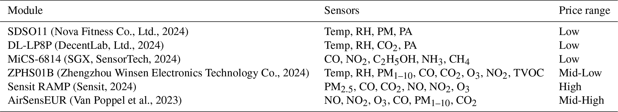
Note that LCSs are designed for basic monitoring at a low cost, which compromises accuracy and durability. In this list, there are several types of LCSs. Optical type sensors, such as SDSO11 (Nova Fitness Co., Ltd., 2024) and DL-LP8P (DecentLab, Ltd., 2024), measure the amount of light absorbed by a given gas. Metal-oxide sensors, such as (SGX, SensorTech, 2024), measure the change in electrical conductivity on a semiconductor due to the presence of certain gases. Usually, sensors of this type are the cheapest and are particularly susceptible to cross-sensitivities. Electrochemical sensors have higher selectivity and are good for measuring specific gases, but they are more expensive. Sensit RAMP (Sensit, 2024) and AirSensEUR (Van Poppel et al., 2023) use this type of sensor. Finally, the ZPHS01B module (Zhengzhou Winsen Electronics Technology Co., 2024) integrates optical, metal-oxide, and electrochemical sensors. It is a Mid-Low price module with the best price/sensor ratio.

Since one of the key points to improve the accuracy of these LCSs is the use of marginal information (such as Temp and RH as well as other AQ pollutants) exploited using AI techniques (Karagulian et al., 2019; Esposito et al., 2016), as mentioned before, it is necessary to use multi-gas modules embedding as many AQ LCSs as possible.

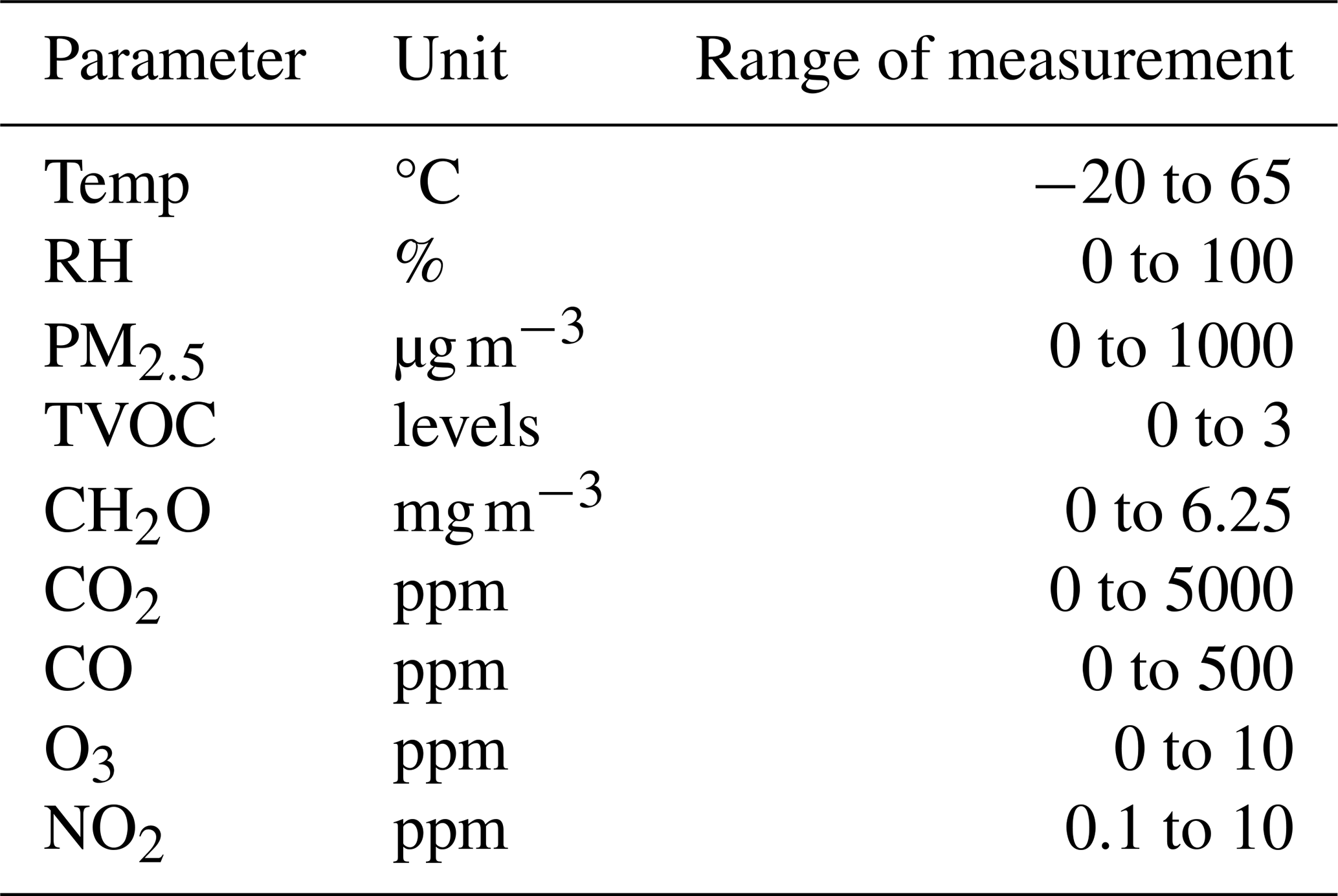
Thus, among the different low-cost alternatives, and taking into account the number of sensors and the price/sensor ratio, the ZPHS01B (Zhengzhou Winsen Electronics Technology Co., 2024) is the AQ sensor module that best meets the needs and objectives of this study at the time of writing, since it embeds nine different sensors: Temp (°C); RH (%); CO, CO₂, NO₂, and O₃, which are measured in parts per million (ppm); formaldehyde (CH₂O), which is measured in mg m⁻³; PM, which is measured in µg m⁻³; and TVOCs, which are measured using four levels according to its concentration (0 – very low, 1 – low, 2 – intermediate, and 3 – high). Table 2 summarizes all this information. Notice that the O₃ sensor used in this module is the electrochemical ZE27-O3 (Corp, 2024), which measures in the range 0–10 ppm with a resolution of 0.01 ppm. It operates with an accuracy of ± 0.1 ppm when the concentration is ≤ 1 ppm and ± 20 % when the concentration is above 1 ppm. Also, notice that the PM readings in this module are given for 2.5 (fine particles with a diameter of 2.5 µm), and PM₁ and PM₁₀ are estimated from the CH_2.5 readings.

Table 2 AQ information from the ZPHS01B module and units.

There are several research works and projects based on this ZPHS01B module. Coto-Fuentes et al. (2022) show the implementation of a device for AQ outdoor evaluation directly using this module without calibration to map AQ pollutants in a metropolitan area. Felici-Castell et al. (2023) use this module in an AQ monitoring network where different neural networks have been trained for forecasting of pollutant concentrations, with an estimation error of 7.2 % on average and where the calibration process is done on a daily basis but is not specified. Vaheed et al. (2022) use this module for indoor AQ monitoring and calculating an AQ index. Antonenko et al. (2023) explain briefly the use of a neural network to determine (classify) types of air: with or without pollution. Kennedy et al. (2021) show a prototype to measure ground to stratosphere AQ using this module in a drone. However, the variability among the individual sensors is high, stressing that the calibration process is complex and has not been done.

Regarding LCS performance analysis, Borrego et al. (2016) conducted a 2-week assessment in Aveiro (Portugal) of various LCS models. Specifically for O₃, the best performance compared to a reference station was achieved by the MiCS-OZ-47 and Alphasense B4 electrochemical sensors, which obtained a coefficient of determination R² values (and MAE in parts per billion, ppb) of 0.77 (7.66) and 0.70 (2.4), respectively.

The calibration process of these LCSs is a challenge, as mentioned before, where ML and deep learning (DL) models can be used. In Wang et al. (2024), a low-cost multi-parameter AQ system based on PM_2.5, PM₁₀, SO₂, NO₂, CO, and O₃ along with Temp and RH is proposed, using and evaluating various calibration algorithms. For O₃, the algorithms are ranked from best to worst fit as follows: RF, K-nearest neighbors (KNN), back propagation (BP), genetic algorithm back propagation (GABP), and multiple linear regression (MLR), with R² values (MAE, in µg m⁻³) of 0.98 (2.88), 0.87 (7.33), 0.83 (11.14), 0.83 (10.90), and 0.74 (13.46), respectively. With a mean O₃ concentration of approximately 70 µg m⁻³, as shown in their Fig. 12, the RF model achieves a MRE of 4.11 %. In Cavaliere et al. (2023), based on O₃ and NO₂ metal oxide sensors, along with Temp and RH, the authors analyzed different calibration options using uni-variate/multi-variate, linear/nonlinear and parametric/non-parametric approaches with algorithms such as linear regression (LR), nonlinear regression (NLR), support vector machines (SVMs), RF, and GB. They concluded that multiple random forest (MRF) achieved the highest accuracy during Phase I (pre-deployment), with an R² of 0.98 and MAE (MRE) of 4.31 (5.74 %), considering a mean O₃ during their deployments of 75 µg m⁻³, depicted in their Figs. 3 and 7. However, in Phase II (field validation) conducted at a different location, the performance worsened, with MAE (MRE) 22.22 (29.62 %) and MLR 12.96 (17.28 %). In this case, MLR provided better results. The authors conclude that MLR may be a more suitable solution for representing physical models beyond the Phase I calibration dataset, demonstrating better transferability across diverse spatial and temporal settings, highlighting that parametric models such as MLR have a defined equation with only a few parameters, making them easier to adjust for potential changes over time. In Wang et al. (2020), the authors propose a category-based calibration approach (piecewise) using ML, which builds separate regression models for different pollutant concentration levels. This proposal is tested on CO and O₃ data from two Chinese cities, Fuzhou and Lanzhou, with good and bad AQ with mean O₃ concentrations of 69.545 and 49.781 µg m⁻³, respectively, for 11 months (48 weeks). The achieved metrics for the best results are given by extreme GB and light GB machine algorithms (outperforming linear regression and RF) with MAE (µg m⁻³) of 10.75 and 10.98, respectively, in Lanzhou city and 13.83 and 14.98 in Fuzhou city, with an MRE greater than 19.88 %. In Zimmerman et al. (2018), calibration models (using 16 weeks of data) are shown to improve sensor performance, highlighting that the RF approach is more robust since it accounts for pollutant cross-sensitivities. Using specific LCSs (RAMP system), they achieve an MRE of 15 % for O₃. In the study performed by Johnson et al. (2018), the calibration of an aerosol sensor for PM_2.5 is carried out by comparing simple linear regression models with GB using the PPD42 PM sensor (Shinyei, 2024). The study concludes that gradient boosting performed better and significantly improved the performance of the sensors, reaching an R² of up to 0.76. Casey et al. (2019) show that neural networks (NNs) generally outperform lineal models to quantify O₃, CO, CO₂, and CH₄ in ambient air using gas sensors integrated into U-Pod AQ monitors. They also highlight that NNs capture the complex nonlinear interactions among multiple gas sensors, considering factors such as Temp, RH and atmospheric chemistry. Also, Esposito et al. (2016) use dynamic NNs for calibration, achieving models with R² (MAE) (in ppb) of 0.69 (7.45) with an MRE of 42 %.

In this context, when using AI techniques for environmental research, it is important to follow the recommendations and good practices given by Zhu et al. (2023) based on a review of more than 148 highly cited research papers. In this paper, it is highlighted that data preprocessing, analysis, and interpretability, such as feature importance analysis (FIA), principal component analysis (PCA), and feature selection (FS), are often overlooked as part of the exploratory data analysis (EDA). A good example of the use of these good practices is shown in Cavaliere et al. (2023). In addition, in Zhu et al. (2023), it is said that the process of optimizing algorithms through the selection of their hyperparameters (hyperparameter optimization, HPO) is neglected in most of the environmental research studies considered. For instance, in Johnson et al. (2018), better results are obtained with GB, but HPO, which could allow further improvements of the results, is not performed in the model. Malings et al. (2019), Wang et al. (2020), and Zimmerman et al. (2018) take into account some aspects related to the data analysis focused on the optimization of the problem, but they do not carry out an HPO. Esposito et al. (2016) carry out a kind of simple HPO based on raw tests of different architectures and modifying hyperparameters such as the number of hidden layers of the model, tapped delay length, and feedback delay line length, and conclude that a dynamic approach to these parameters improves the results with respect to a static approach without changing the value of these parameters.

Regarding the selection of parameters, Johnson et al. (2018) do not perform an analysis using techniques such as the aforementioned FIA and FS, but a sensitivity analysis using different meteorological variables (such as Temp and RH), determining that it is useful information for GB. In Malings et al. (2019), the quantification of the importance of the model variables is mentioned as a means to understand which information is useful, concluding that for RF, it is very helpful to add additional information apart from AQ measurements, such as Temp and RH. Esposito et al. (2016) and Wang et al. (2024) do not include a specific analysis of the relative importance of different variables or features. However, a good example of FS is depicted in Okafor et al. (2020), where it is shown that identifying the environmental factors affecting LCSs is crucial for improving data quality using data fusion and ML. These factors are then incorporated into the development of the calibration model.

In conclusion, in order to increase the resolution of city-scale AQ monitoring according to the recommendations given by Directive 2008/50/EC (2008) as mentioned before, it is necessary to perform a calibration process of these LCSs. In this scenario, we focus on O₃ calibration using ensemble ML techniques to minimize inaccuracies and nonlinearities, comparing four different models, considering different environmental variables as well as metadata mainly to account for sensor aging effects. For this purpose, it is necessary to carry out a thorough data treatment with good practice criteria (Zhu et al., 2023) including HPO, FIA, and/or FS, which are usually overlooked. In a scenario with low O₃ concentration, we achieve interesting results compared with related works, as shown in Sect. 4.

3 Building the datasets and using machine learning algorithms

In this section, we explain the process of gathering AQ monitoring information from a prototyped low-cost internet of things (IoT) node based on the ZPHS01B AQ module, how it is deployed, and how the datasets are built to apply ML techniques for calibration purposes. For this, we generate two datasets in the city of Valencia (Spain) at two different locations with the same characteristics (close to the ring road but separated by 4.1 km), covering periods of 165 d and 239 d.

3.1 Building the datasets

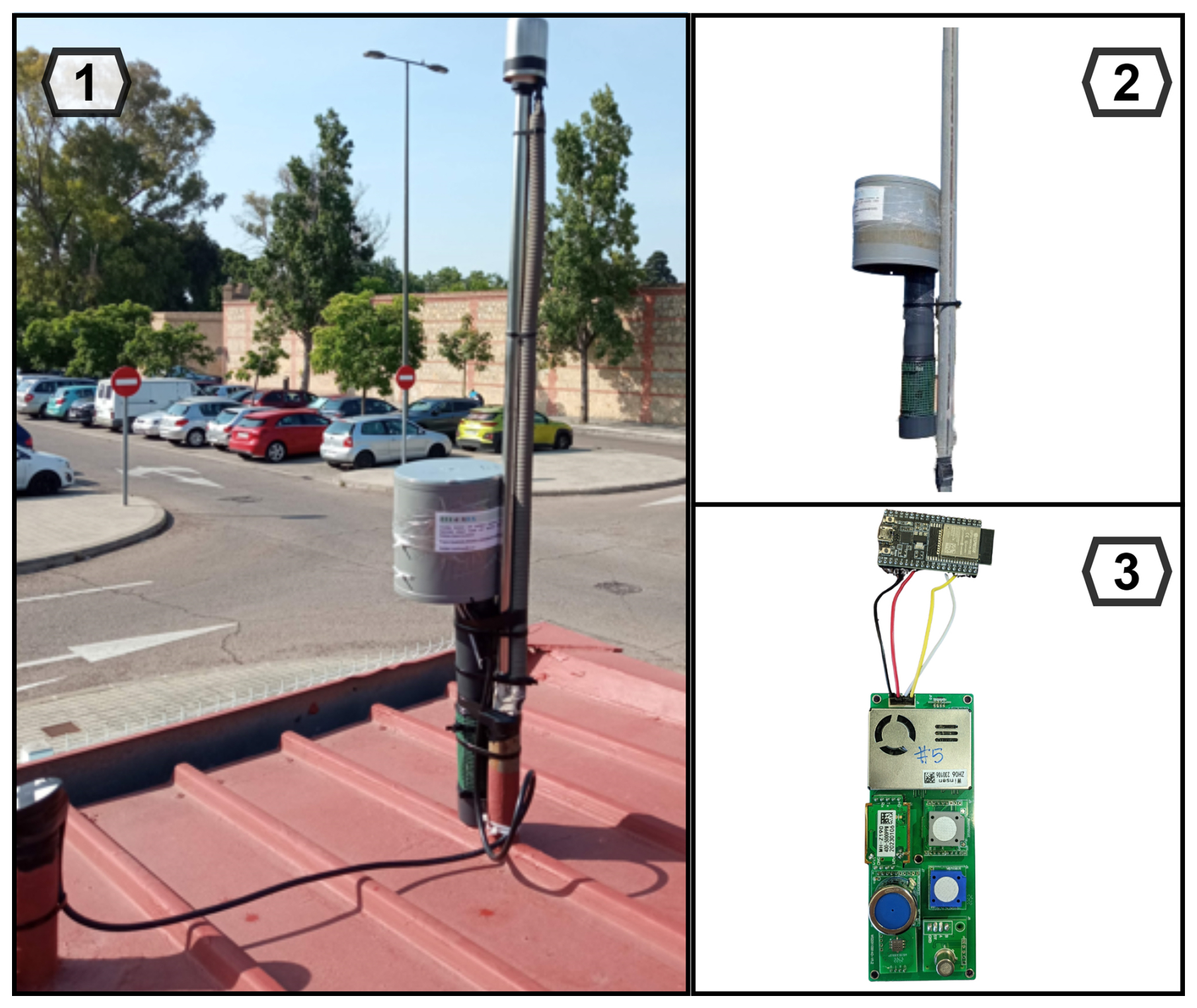
To calibrate the O₃ sensor from the ZPHS01B module, we require a dataset (named dataset-1) (Montalbán Faet et al., 2025a) to train various ML models. For this purpose, we use as reference values O₃ concentration readings from the standardized AQ station in the Valencian AQ Monitoring Network (VAQMN) at Bulevar Sur (Valencia, Spain) managed by Generalitat Valenciana (GVA) with latitude and longitude 39.450389 and −0.396324, respectively, as shown in Fig. 1. In this picture, the IoT node is shown placed 4 m above ground level in accordance with Directive 2008/50/EC (Directive 2008/50/EC, 2008). These reference values are given in µg m⁻³, periodically averaging every 10 min. The AQ station data is retrieved from Generalitat Valenciana (2025a). Dataset-1 includes 165 d from 8 June to 20 November 2023. The ZPHS01B module's readings are taken at a rate of 10 samples per minute, one sample every 6 s. Notice that, as a first approach, creating a dataset with different locations is not recommended, as it could alter environmental conditions and interfere with the training process. That is the reason we generate two different and independent datasets.

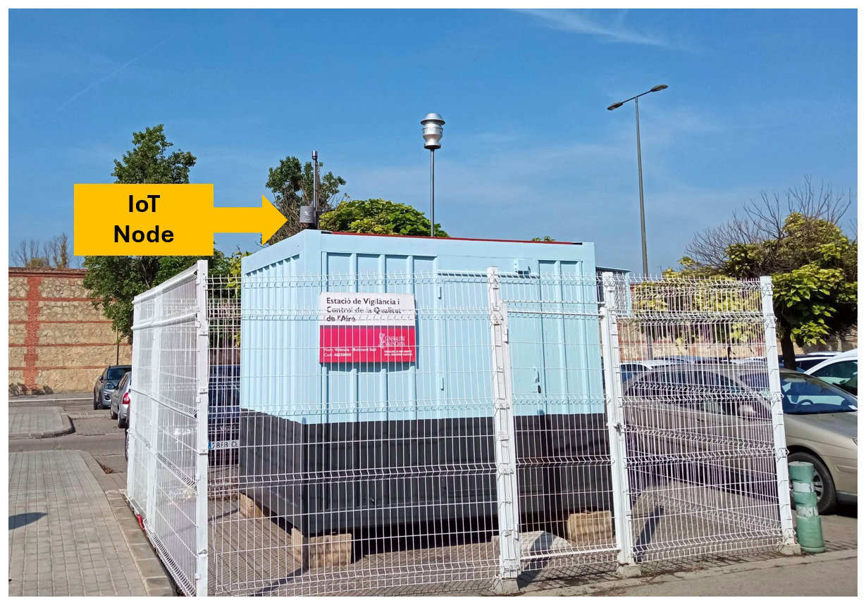
Figure 1 Detail of the standardized AQ monitoring station and the AQ node with a ZPHS01B module located at Bulevar Sur (Valencia, Spain).

Table 3 presents the structure and main statistics of dataset-1. The units used for O₃ concentration from the standardized and regulated station are µg m⁻³, while the ZPHS01B module uses ppm. Both units are typically used in a formal and academic context, but we need to standardize them. The formula used to carry out this conversion for O₃ is in standard conditions: “Concentration (µg m⁻³) = molecular weight (48 g mol) × concentration (ppb) ÷ 24.45”, that is, 1 ppb is 1.96 µg m⁻³ (Breeze Technologies, 2024).

Table 3 Summary of main statistics of dataset-1: minimum (Min.), maximum (Max.), mean (Mean), standard deviation, median absolute deviation (MAD), percentage of samples taking different values (Diff.) and high correlation (High corr.)

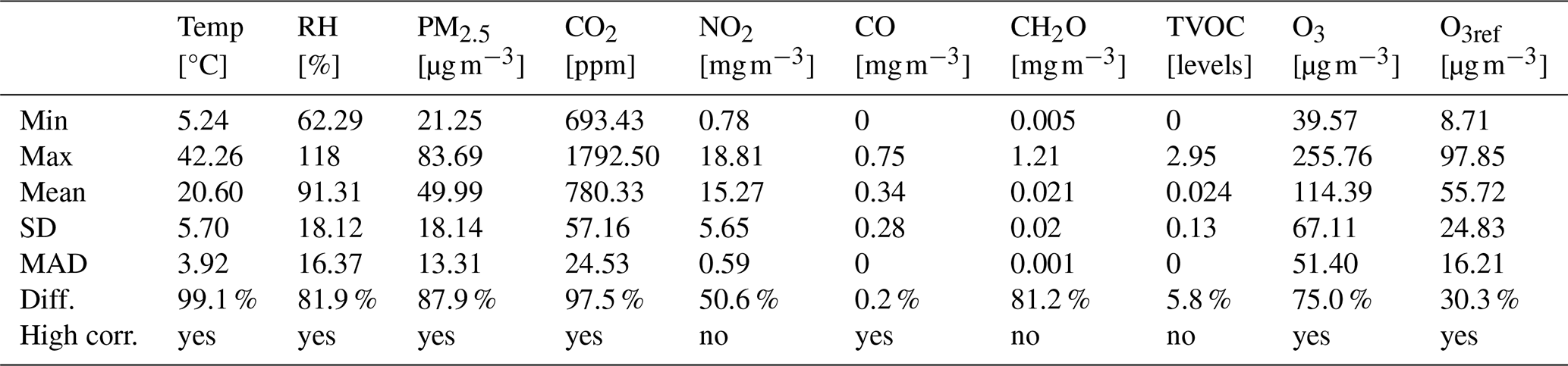
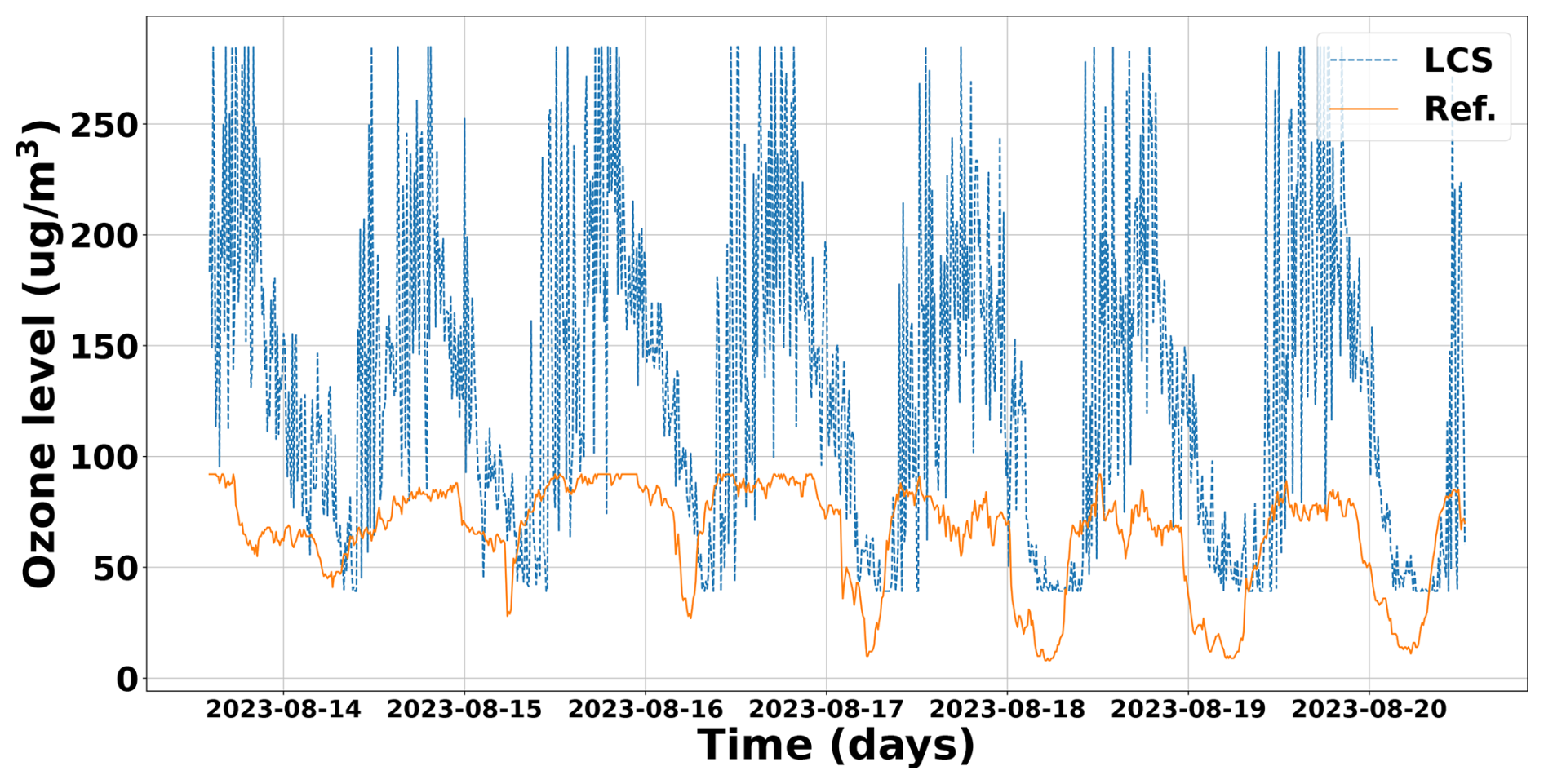
Figure 2 shows the IoT node (and its housing) that keeps the ZPHS01B module within a PVC pipe with a small fan at the top to ensure air circulation. In the head of this node is placed the microcontroller that sends data via the LTE-M communications. Further detail about the features of this node is given in Meneses-Albala et al. (2025).

Figure 2 (1) AQ IoT node; (2) deployment detail; (3) hardware detail.

In addition, in order to test the proposed models in this paper and their generalization in Sect. 4, we have used another dataset (named dataset-2) with two different AQ IoT nodes (Node 1 and Node 2) from the standardized AQ monitoring station called Moli del Sol (Valencia, Spain) with latitude and longitude 39.48113875, −0.40855865 (Montalbán Faet et al., 2025b). This station is 4.1 km away from the previous one. Its data is retrieved from Generalitat Valenciana (2025b). This dataset includes 239 d from 31 May 2024 to 25 January 2025. From now on, we will refer to dataset-1 as the dataset, except in Sect. 4 where we generalize the models with dataset-2.

3.2 Analyzing the dataset

The initial data collection (dataset-1) is based on 6 s frequency samples. Based on this collection, three datasets have been created by averaging data over different time monitoring intervals: 10 min, 30 min, and 1 h, with 23 496, 7843, and 3922 samples, respectively. The lowest 10 min interval is given by the standardized AQ station, and 30 min and 1 h are common time bases for AQ parameters. Although they are not large datasets, they are sufficient, as shown in Zhu et al. (2023), due to the relationship (ratio) between sample size and feature size, with four features in total, as seen next. This ratio is called the sample-size to feature-size ratio (SFR), with an SFR higher than 500 recommended. More detail is given in Sect. 3.3.

Initially, the datasets were cleaned of invalid data. Notice that from the readings of the standardized AQ station, we had 275 not-a-number (NaN) results during this period, that, in our case, were replaced using the quadratic interpolation method, since experimentally it gave better results and made the interpolation closer to the ozone signal. This explanation for preparing the dataset, also known as missing data management (MDM), is recommended according to Zhu et al. (2023).

Table 3 shows a summary of the main statistics of dataset-1. For each parameter, the table shows the minimum value (Min.), maximum value (Max.), mean value of all entries (Mean), standard deviation (SD), median absolute deviation (MAD), and the percentage of samples taking different values (Diff.) and high correlation (High corr.) with others.

From these results, it is worth mentioning that the CH₂O, CO, TVOC, and NO₂ sensors do not seem to be working properly in the ZPHS01B module; CH₂O, CO, and TVOCs are almost always stuck to values close to zero, seeming to not excite at normal concentrations, with very low variability. On the other hand, the NO₂ sensor appears saturated. Thus, in practice, the number of features used from Table 3 is five; that is, from the initial nine (the reference is not included), we remove these four: CH₂O, CO, TVOCs, and NO₂. Also, the RH sensor has a positive offset, as we can see from the maximum value, 118 %.

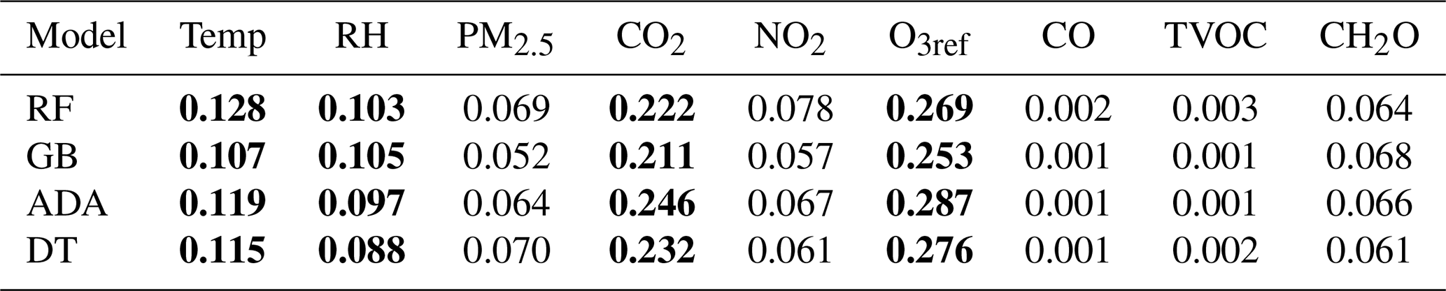
Figure 3 shows the O₃ readings in µg m⁻³ from the LCSs and the regulated station (reference) for 1 week. It can be seen that there is an offset in the LCS readings over the ones from the reference. Also, it is clear how the O₃ LCS captures the trends, useful information for the ML models. A further analysis of these sensor readings in the frequency domain is shown in Appendix A, where a repeated daily pattern is clearly observed, as expected, based on how O₃ is generated from other pollutants produced by road traffic and complex photochemical reactions, as discussed in Sect. 1.

Figure 3 O₃ readings in µg m⁻³ from the LCS and reference for 1 week.

3.3 Feature importance analysis and selection

FIA and FS play crucial roles in ML models, especially in environmental research, by helping to preserve essential features (variables), reduce noise, and enhance model efficiency, which is particularly relevant when dealing with a small set of samples or large numbers of variables (Zhu et al., 2023).

Table 4 shows the normalized output of the FIA using the scikit-learn library (Pedregosa et al., 2011) for the parameters complementary to O₃ for each ML model used. In order to determine the most useful parameters for the models, a threshold is established at 0.08, that is, 8 % of importance. These parameters are in bold. Notice that the set of parameters with the highest importance is repeated for all models: Temp, RH, CO₂, and O₃.

Table 4 FIA of ozone's complementary parameters for RF, GB, ADA, DT, the selected ones in bold, contribution higher than 0.8.

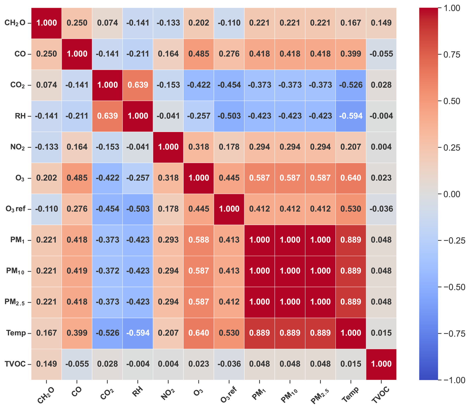
With regard to FS, Fig. 4 shows the correlation matrix for these variables. There is a high correlation among all PM_x readings because all of them are calculated directly from PM_2.5 (Zhengzhou Winsen Electronics Technology Co., 2024). Also, from this analysis, we stress that Temp and RH are the best correlated with the rest of the variables, as well as O₃ LCS, O₃ reference, PM_2.5, and CO₂, but these have a lower correlation. Thus, all this information is very valuable for training the ML models.

Figure 4 LCS readings and O₃ reference correlation matrix.

3.4 Applying machine learning algorithms

As mentioned before, in environmental research, the use of ML algorithms, in particular ensemble models, has increased significantly compared with DL (Zimmerman et al., 2018). Some of the most popular ensemble algorithms are RF or GB related models (Obregon and Jung, 2022). Furthermore, based on our experience, we recognize that in AQ monitoring scenarios using LCSs such as the ZPHS01B module, datasets are often limited and constrained, which affects the use of DL techniques as they usually tend to overfit.

This paper evaluates these ensemble ML algorithms: RF, GB, and ADA algorithms, implemented in the scikit-learn (Pedregosa et al., 2011) library (in the ensemble submodule), which offers efficient solutions for time series regression problems such as this one. These evaluated methods exhibit the ability to handle nonlinear relationships and adapt to changing patterns over time. In addition, the DT model, belonging to the tree submodule of scikit-learn, is also evaluated, since it is a common base of this type of ensemble algorithm.

To optimize these models as indicated in Zhu et al. (2023), there are different techniques and tools for carrying out the HPO, with GridSearch (Pedregosa et al., 2011) being the most commonly used method to obtain a good configuration for these algorithms. GridSearch in scikit-learn is a hyperparameter tuning technique that exhaustively searches through a user-defined hyperparameter space to find the optimal combination for an ML model. These hyperparameters are external specific model configuration settings. This method systematically evaluates the model's performance across all possible user-defined hyperparameters using cross-validation, aiming to identify the configuration that maximizes estimation accuracy or minimizes a specified loss function. We choose this method because of its higher flexibility compared with other tools, such as RandomSearch (Pedregosa et al., 2011), which has a more random approach.

Next, we discuss the different supervised ML algorithms used and the selection of the different hyperparameters, taking into account the best results of R², root mean square error (RMSE), and MAE.

3.4.1 Random forest (RF)

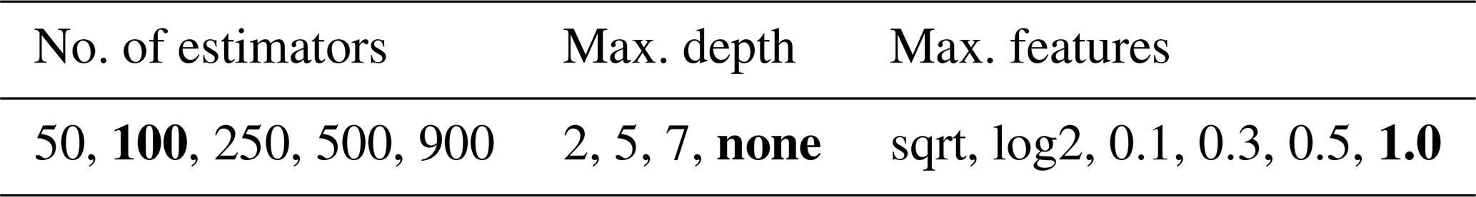
RF is an ensemble algorithm that relies on constructing multiple DTs during training. Each tree is trained on a random subset of the dataset, and the final predictions are obtained by averaging the individual predictions for all of them. This “forest” approach helps to mitigate overfitting and improves the model's generalization. Furthermore, introducing randomness in the selection of features and samples during tree construction contributes to a more robust and accurate model for regression tasks. Table 5 shows the hyperparameters evaluated, with the best option in bold. The number of estimators refers to the number of trees in the forest, while the maximum depth refers to the maximum depth of the tree. The maximum features variable determines the upper limit on the number of features to consider when splitting a tree into two child nodes during the tree construction process. Note that as the number of estimators does not have a significant role in this use case, we use the default value, 100.

Table 5 RF hyperparameters evaluated on GridSearch showing in bold the combination that gives the best results in terms of R², RMSE, and MAE.

3.4.2 Gradient boosting (GB)

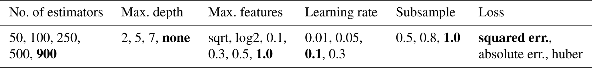
GB is an ensemble algorithm based on the iterative construction of weak DTs, which are sequentially aggregated to enhance the predictive capability of the model. In each iteration, it focuses on correcting the residual errors of the existing model by fitting a new DT to capture the deficiencies of the current model. The weighting of individual trees is determined by a learning rate, and the final output of the model is the weighted sum of predictions from all these trees. This gradual building process and the ability to handle nonlinear relationships in the data make GB effective for regression tasks. Table 6 shows the hyperparameters evaluated, with the best option in bold. In addition to the previous hyperparameters, in this case, the loss hyperparameter refers to the loss function to be optimized, while the learning rate reduces the contribution of each tree according to the value of the variable. The subsample hyperparameter represents the fraction of samples that will be used to adjust the individual base learners, and if it is less than 1.0, it results in stochastic gradient boosting (SGB).

Table 6 GB hyperparameters evaluated on GridSearch showing in bold the combination that gives the best results in terms of R², RMSE, and MAE.

3.4.3 Adaptive boosting (ADA)

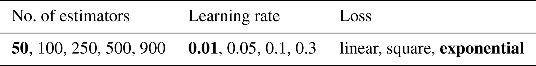
ADA is an ensemble algorithm whose primary goal is to improve the predictive accuracy by combining multiple weak regression models. When training, ADA assigns weights to data instances, giving more emphasis to observations that were poorly predicted in previous iterations. Its construction involves the sequential aggregation of regression models, each fitted to correct errors from the existing combined model. The final model is a weighted combination of individual predictions from the base models. ADA is particularly effective in enhancing generalization capability and reducing overfitting in regression tasks. Table 7 shows the hyperparameters evaluated, with the best option in bold. In this model, a key concept is to run the optimization process related to the estimator variable, which by default is an instance of type DecisionTreeRegressor, initialized with a maximum depth value of 3. If the value of this hyperparameter is not modified, this model is largely constrained. Also, notice that as the number of estimators does not have a significant role on this use case, we use the default value of 50 estimators. The other hyperparameters have the same meaning in this model.

Table 7 ADA hyperparameters evaluated on GridSearch showing in bold the combination that gives the best results in terms of R², RMSE, and MAE.

3.4.4 Decision tree (DT)

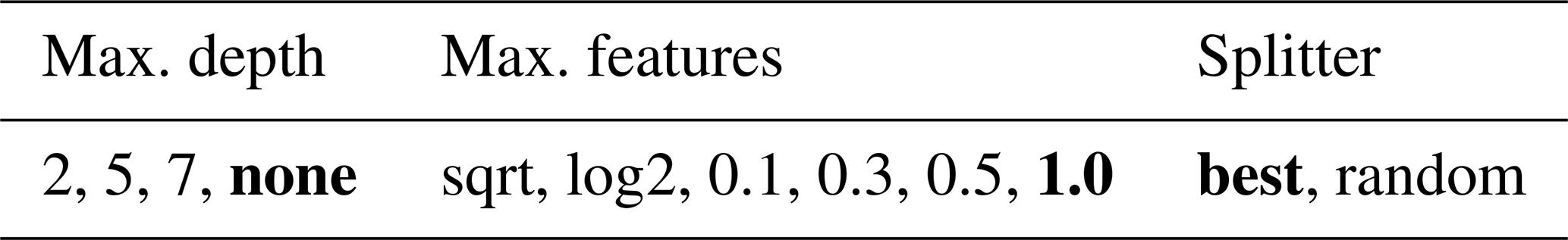
DT is an algorithm that recursively partitions the dataset based on features, aiming to create a hierarchical structure of decision nodes to make predictions. Table 8 shows the hyperparameters evaluated, with the best option in bold. The splitter hyperparameter indicates which strategy is used to perform the splitting at each node.

Table 8 DT hyperparameters evaluated on GridSearch showing in bold the combination that gives the best results in terms of R², RMSE, and MAE.

4 Results

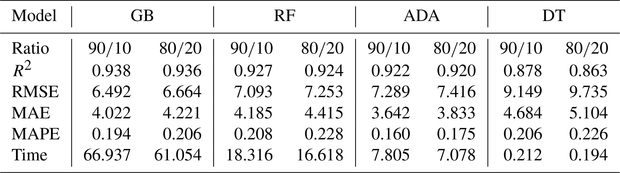
We evaluated the performance metrics of these ML models under different configurations (in terms of R², RMSE and MAE in µg m⁻³, mean absolute percentage error (MAPE), and execution time in seconds), with the optimized hyperparameters that achieve higher R² and lower errors. Also, we used the three different datasets given by different monitoring intervals: 10 min, 30 min, and 1 h, as depicted in Sect. 3.2. We tested different training–test ratio percentages from these datasets: 60 %–40 %, 70 %–30 %, 80 %–20 %, and 90 %–10 %, denoted as $\mathrm{60}/\mathrm{40}$, $\mathrm{70}/\mathrm{30}$, $\mathrm{80}/\mathrm{20}$, and $\mathrm{90}/\mathrm{10}$. Note that when we split the dataset for training and testing, both sets remain independent and isolated. However, during the training process itself, the dataset is further divided into two parts: one for training and the other for validation. By default, we allocate 80 % of the data for training and 20 % for validation. In this process, the training and validation datasets are combined across different iterations. From all of them, we achieved the best results in terms of these performance metrics with a $\mathrm{90}/\mathrm{10}$ training–test ratio with a monitoring interval of 10 min, as shown in Table 9. Also, from the analysis carried out in Sect. 3.3, for the feature selection, we proceed in this section with the features that also provide the best results, based on [date, O₃, Temp, RH]. Notice that “date” is included as metadata to account for the aging effect and to improve the models following the traffic pattern. We see that the fewer the features, the better the results, i.e., increased SFR. Then, other dimensionality reduction techniques are not required. If we add more features that are not so significant, it makes the dataset poorer. Notice that the performance metrics shown in Table 9 are the weighted average of each metric over 100 different iterations by changing the content of the training and test set to obtain results with the minimum bias possible.

Table 9 Performance metrics for HPO models with $\mathrm{90}/\mathrm{10}$ and $\mathrm{80}/\mathrm{20}$ (training $/$ testing) ratio.

During the training process, we can observe the convergence of the performance metrics, which provides information about overfitting, considering both the training and validation datasets. Appendix B includes this information analyzing both R² and RMSE across different iterations. Each model uses its own reference hyperparameter for convergence. In particular, in Fig. B1, we observe the fit of the model in terms of R², with a better fit with training than with validation, as expected, and similarly for RMSE, as we can see in Fig. B2. It should be noted that the convergence process with training does not reach a perfect fit in any case, which justifies and supports initially the conclusion that there is no overfitting in the models. Moreover, we see that the achieved R² and RMSE scores for both training and validation are better than the values shown for testing in Table 9, because the testing dataset does not participate in the training process.

It is worth mentioning that the improvement achieved by HPO is greater in GB and ADA models than in RF and DT, which are already well optimized with default values. In particular, for the optimized GB and ADA models, R² is improved by 42 % and 182 %, respectively, while RMSE is reduced by 57 % and 66 %. However, the execution time required for training is influenced by HPO, increasing to 66.937 s and 7.805 s for GB and ADA, respectively, as shown in Table 9. We highlight that RF and DT are already well optimized, and their execution times remain unchanged between the default and optimized versions.

Figure 5 shows the calibration process for both the default and HPO models vs. O₃ reference given by the different algorithms.

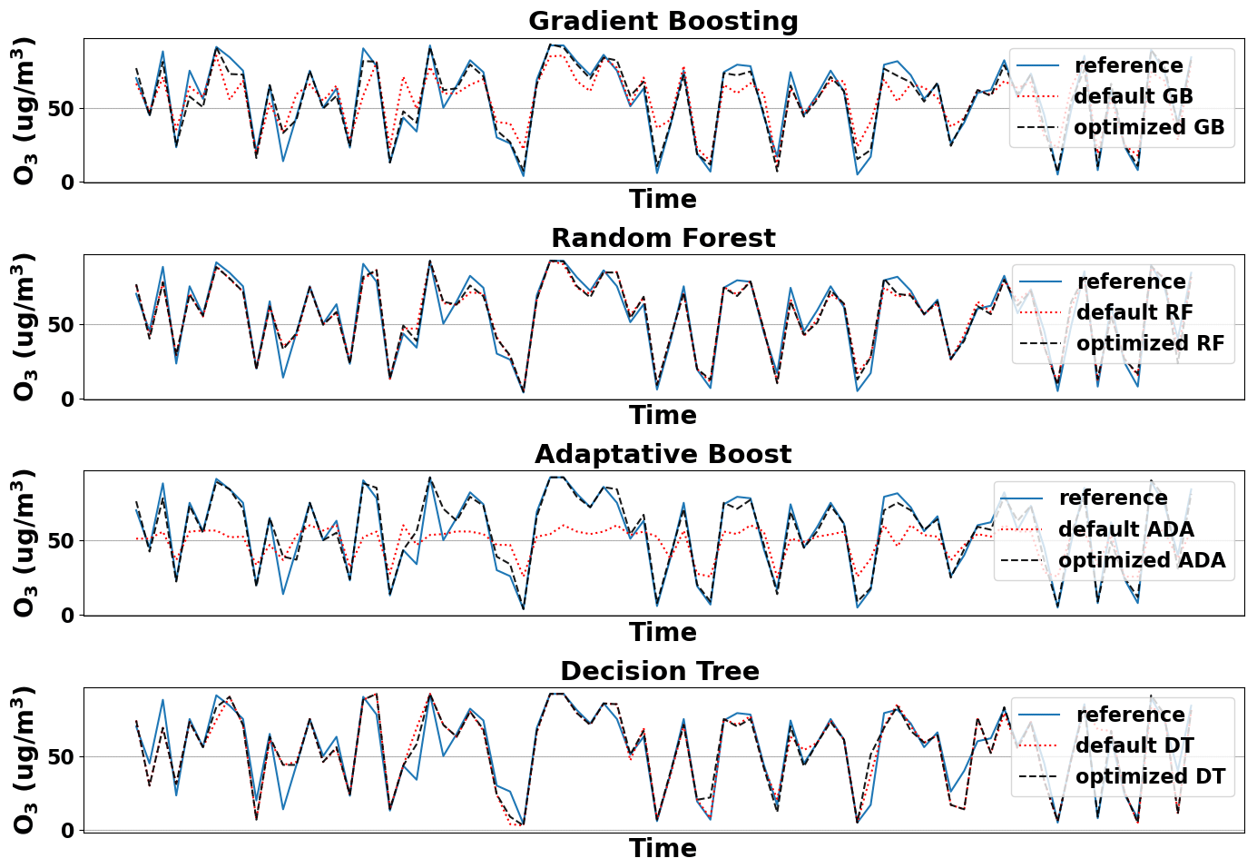
Figure 5 Ozone calibration done with default and optimized models with $\mathrm{90}/\mathrm{10}$ (training $/$ testing) ratio dataset.

However, it is common to use an $\mathrm{80}/\mathrm{20}$ training–testing ratio (Zhu et al., 2023). For this ratio, Table 9 also shows these results with the optimized models by HPO, where the GB model is the best one again, as with the previous $\mathrm{90}/\mathrm{10}$ ratio.

A summary of these metrics (R² and errors) for the GB model, with different monitoring intervals and different training–testing ratio percentages, is shown in Fig. 6. We can see that when increasing the training percentage, the trend is to improve the accuracy of the model (R² getting closer to 1) and to slightly reduce the errors but increase the training time, as could be expected. Similar behaviors are exhibited by the other models, particularly the ADA model. Regarding overfitting, Fig. 6 shows that the error difference between using 90 % and 60 % of the data for training (the maximum and minimum percentages, respectively) is approximately 2 % in the worst-case scenario (1 h dataset). This suggests that overfitting is not significant in the proposed model, as we mentioned before, during the convergence process shown in Appendix B.

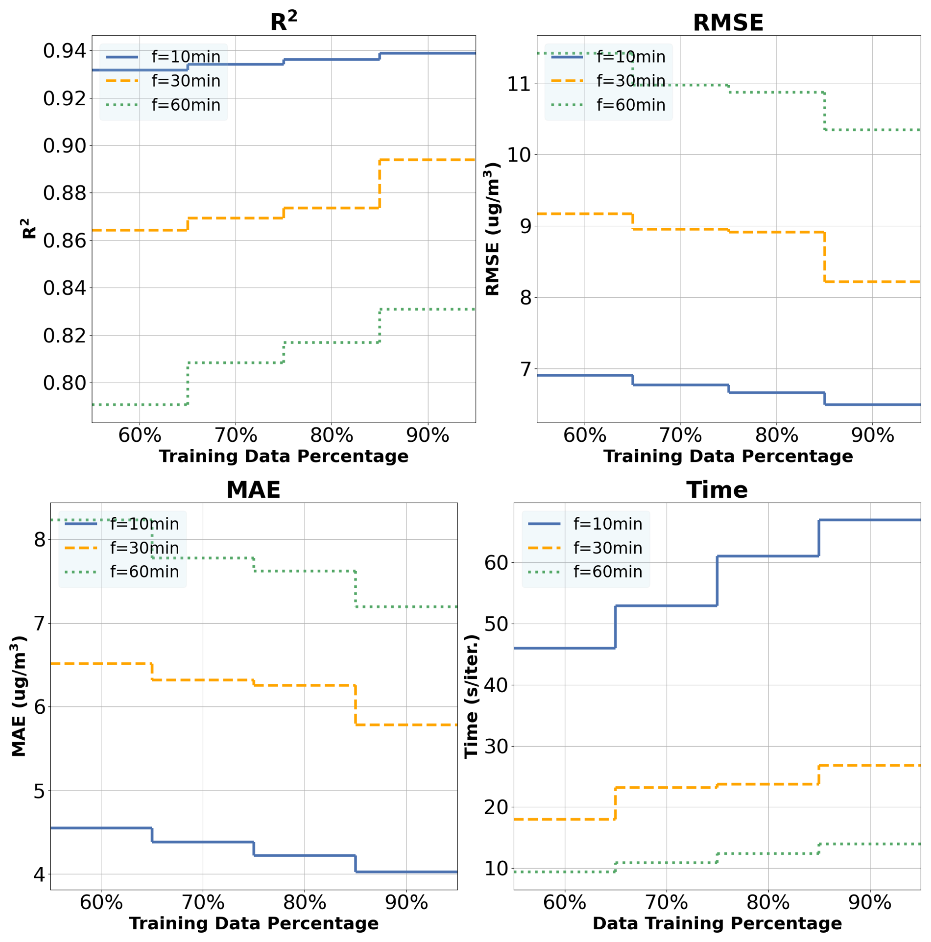
Figure 6 Ozone estimation analysis for GB default and optimized models with different % training datasets and monitoring intervals.

In terms of generalization, as mentioned in Sect. 3.1, we checked the same proposed models with dataset-2 under the same conditions, with a $\mathrm{90}/\mathrm{10}$ (training $/$ testing) ratio. In Fig. 7, we summarize the performance metrics given by the best model based on GB for dataset-1 and for Node 1 and Node 2 from dataset-2. In particular, if we focus on MAE, we see that Node 2 performs slightly better than Node 1 in dataset-2, likely due to manufacturing variations associated with their low cost. We also see that the results from dataset-1 are between these two, validating its generalized behavior. In terms of RMSE, the results from dataset-2 with both nodes is slightly better since it is larger. In all these cases, R² is higher that 0.938.

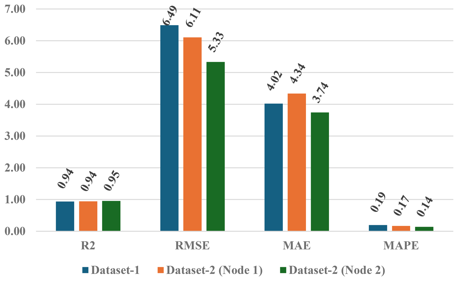
Figure 7 Performance metrics comparison using GB_optimized algorithm with $\mathrm{90}/\mathrm{10}$ (training $/$ testing) ratio over dataset-1 and dataset-2 (Node 1 and Node 2).

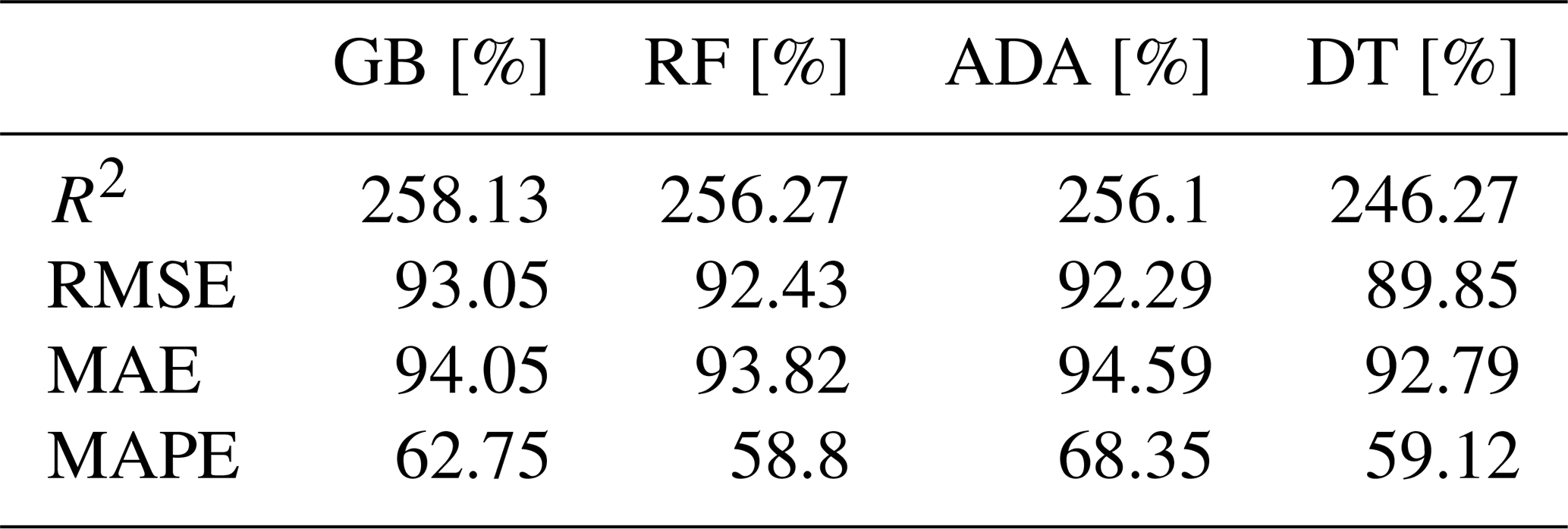
In Table 10, we show the improvement in percentage using the different ML models for the calibration process from the LCS raw readings of the module, highlighting the better performance of the GB model compared with the other models. Notice that with this GB model, the initial MAE from the raw readings was 67.59 µg m⁻³ reducing to 4.022 µg m⁻³, that is, an improvement of 94.05 % as depicted in the table.

Table 10 Improvement (in %) of O₃ calibration from the raw readings with the different optimized models.

Finally, in Table 11, we compare our models for O₃ calibration for LCSs against related works with a similar approach, highlighting the location, platform (and sensors used), R², and MRE along with additional comments about the detail of the models used and dataset duration. First, we must stress that the starting point of the selected papers is slightly different to ours, since these studies have used more reliable and expensive LCSs, approximately 10 times more expensive than the ZPHS01B module. Moreover, since ML-based algorithms show the best results, as discussed in Sect. 2, we have focused exclusively on them, evaluating up to four different models, whereas other studies have considered only one or two. Our model, in particular GB with four features (including “date” as metadata), as shown in Sect. 3.3, achieves a MRE of 7.21 % (given by MAE 4.022 µg m⁻³ with $\mathrm{90}/\mathrm{10}$ dataset, Table 9; and the mean O₃ value of 55.72 µg m⁻³, Table 3). Also, not all of these works follow and discuss an structured EDA with FIA, FS, and HPO. In particular, when compared to the first two works with slightly better results, in Wang et al. (2024), we observe higher O₃ values, with mean values higher than 70 µg m⁻³, while in our case we have lower levels (55.72 µg m⁻³), as well as there not being a complete EDA. It is important to note that these sensors perform worse at low concentrations than at high ones due to their sensitivity limitations and the weakness of the signals generated, as well as interference from other pollutants. Finally, in Cavaliere et al. (2023), although the authors use a complete EDA, they only use two sensors (NO₂ and O₃) apart from Temp and RH, and the aging effect is considered a posteriori, while this information is included in our case by including the date in our models, which also detect other patterns derived from road traffic.

Wang et al. (2024)Cavaliere et al. (2023)Wang et al. (2020)Zimmerman et al. (2018)Esposito et al. (2016)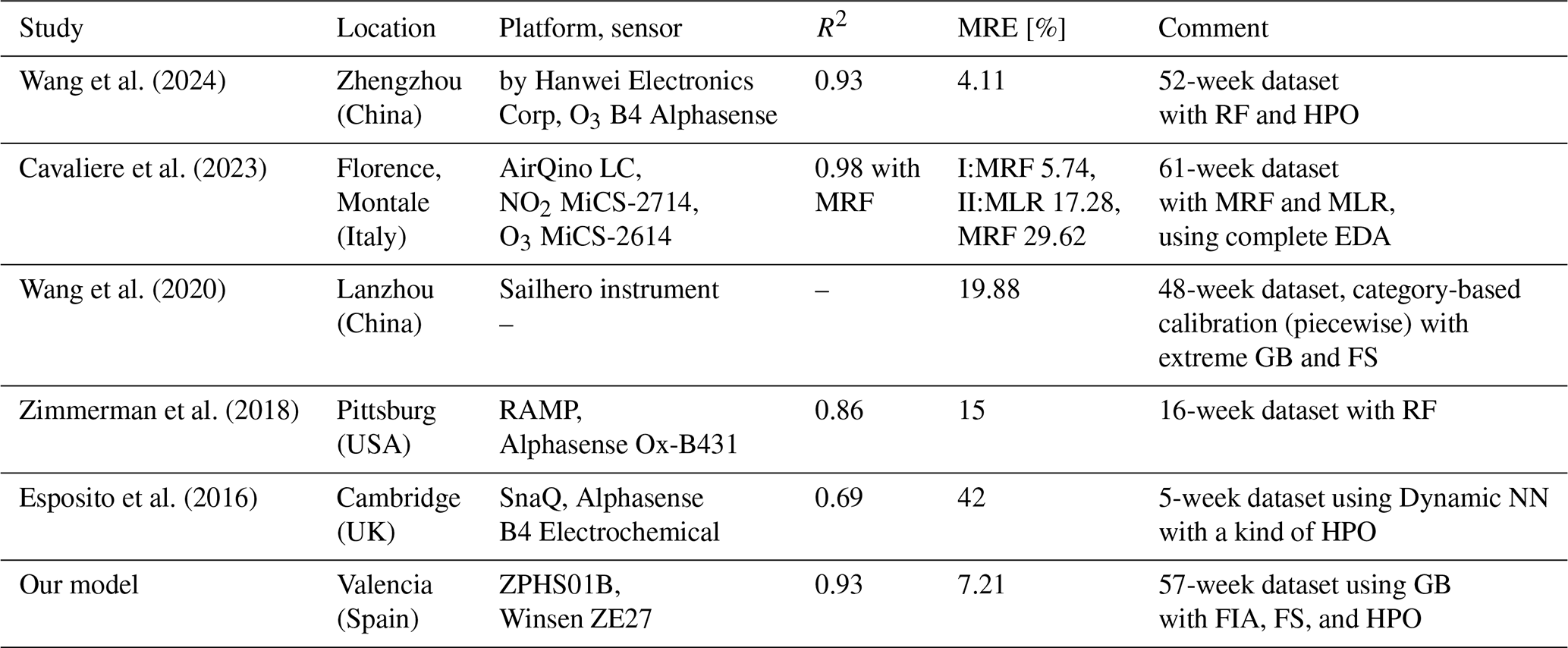

Table 11 Comparison with similar related works.

5 Conclusions

This paper focuses on ground-level ozone (O₃) as it serves as an indicator of other pollution levels in urban areas using LCS nodes based on the ZPHS01B module. These nodes will enable an increase in the spatial sampling of AQ monitoring in cities, following the interests of AQG (WHO Regional Office for Europe, 2021) and in line with the future plans of the related directives, ideally at least one sample per 100 m², according to Annex III-B of the European Parliament Directive (Directive 2008/50/EC, 2008).

Given the low accuracy and nonlinearities of these nodes' sensors, we employed ML models (particularly DT and the ensemble algorithms GB, RF, and ADA) after thorough data analysis, considering additional environmental information and including metadata to account for the aging effect and detect other patterns derived from road traffic; we reduced the estimation error by approximately 94.05 %, and more than 89 % in the other models. In particular, using the GB algorithm, we achieved an MAE of 4.022 µg m⁻³ and a MRE of 7.21 %, outperforming related works while using a module approximately 10 times less expensive.

Initially, we used a dataset spanning 165 d (with low O₃ concentrations and a mean value of 55.72 µg m⁻³) with different monitoring intervals, giving the best results when using a 10 min monitoring interval, as could be expected. If we use higher monitoring intervals (30 min or 1 h), we see that we start losing details, smoothing the dataset and overlooking different behaviors that in the ML process help to reduce the prediction error. For the training process, we carried out several techniques (FIA and FS) in order to select the most relevant features, applying HPO within the different models, with different percentages for training and testing.

Also, we checked that for the ZPHS01B module and O₃ calibration, the 165 d of dataset-1 provided sufficient information to generalize the proposed models, comparing with dataset-2 of 239 d. This aligns with the SFR recommended values according to Zhu et al. (2023). Thus, given the features and characteristics of this module, the original dataset (165 d) contains enough information to generalize the behavior of the O₃ sensor and its response.

As future work, we plan to expand the dataset and include complementary parameters, such as wind speed or additional metadata variables, to increase the accuracy of these models. In addition, we will focus on the design of new calibration and forecasting algorithms for the different sensors embedded in the low-cost ZPHS01B module in order to improve AQ monitoring resolution.

Appendix A: Spectral analysis for low-cost O₃ readings from the ZPHS01B module

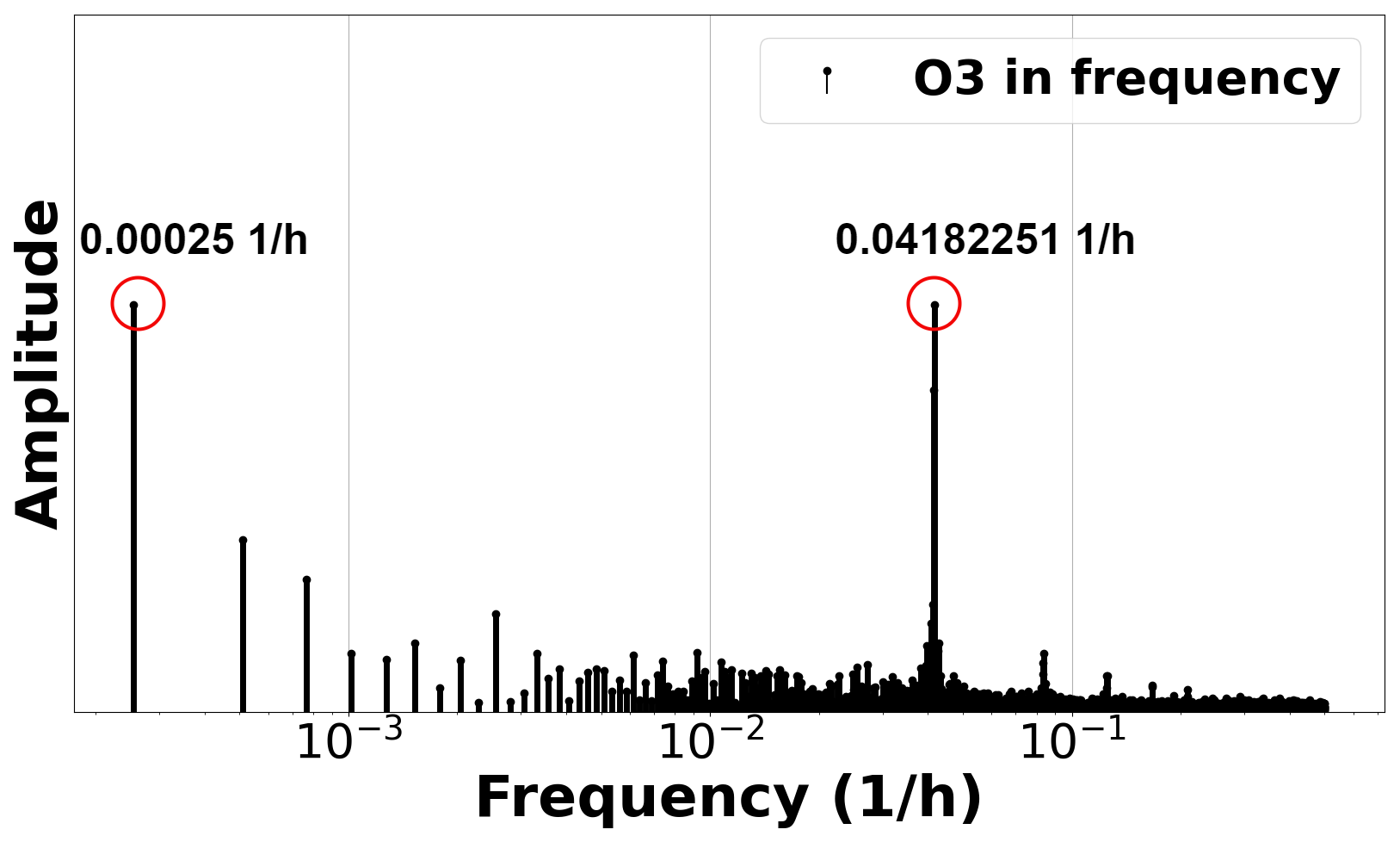
To characterize the measurements of O₃, we carry out a discrete Fourier transform (DFT) analysis to see the changing patterns. DFT is a mathematical technique that transforms a discrete signal from the time domain to the frequency domain. Figure A1 shows the peaks obtained from the O₃ signal. There are two main peaks and their harmonics. The first peak appears in the frequency f = 0.00025 $\frac{\mathrm{1}}{h}$, which corresponds to a period of 4000 h, 5.56 months, that is, the total duration of dataset. The second peak indicates and reveals a relevant frequency component at f = 0.04182251 $\frac{\mathrm{1}}{h}$, which represents a period of 23.91 h (approximately 1 d). Thus, there is an O₃ pattern that is repeated every day, as could be expected in a city, based on how it is generated from road traffic by combustion engines as discussed in Sect. 1.

Figure A1 DFT of O₃ readings from LCS.

Appendix B: Model convergence results

In this appendix, we plot R² and RMSE across different iterations during the training process, with training and validation datasets. Each model uses its own reference hyperparameter for convergence. In Fig. B1, we observe the fit of the model in terms of R², with a better fit with training than with validation, as expected, and similarly for RMSE, as we can see in Fig. B2. It should be noted that the convergence process with training does not reach a perfect fit in any case, which justifies and supports initially the conclusion that there is no overfitting in the models.

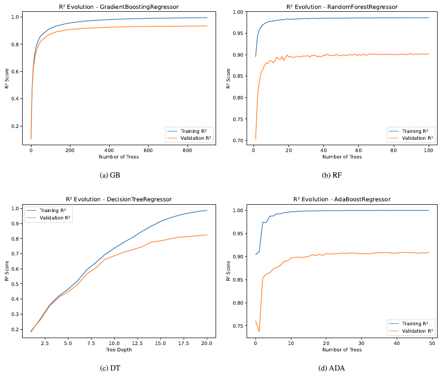
Figure B1 Convergence of R² across different iterations for training and validation for the models with their main reference hyperparameter.

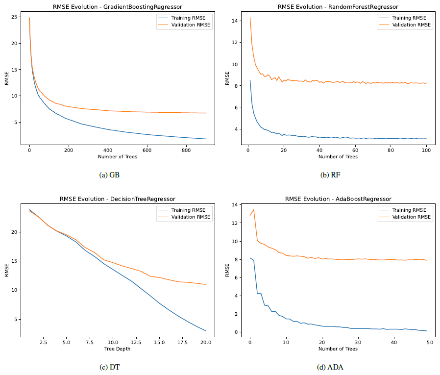
Figure B2 Convergence of RMSE across different iterations for training and validation for the models with their main reference hyperparameter.